Generate, Transduct, Adapt: Iterative Transduction with VLMs

Abstract

Transductive zero-shot learning with vision-language models leverages image-image similarities within the dataset to achieve better classification accuracy compared to the inductive setting. However, there is little work that explores the structure of the language space in this context. We propose GTA-CLIP, a novel technique that incorporates supervision from language models for joint transduction in language and vision spaces. Our approach is iterative and consists of three steps: (i) incrementally exploring the attribute space by querying language models, (ii) an attribute-augmented transductive inference procedure, and (iii) fine-tuning the language and vision encoders based on inferred labels within the dataset. Through experiments with CLIP encoders, we demonstrate that GTA-CLIP, yields an average performance improvement of 8.6% and 3.7% across 12 datasets and 3 encoders, over CLIP and transductive CLIP respectively in the zero-shot setting. We also observe similar improvements in a few-shot setting. We present ablation studies that demonstrate the value of each step and visualize how the vision and language spaces evolve over iterations driven by the transductive learning.

1 Introduction

Recent advances in vision-language models (VLMs) have enabled zero-shot image understanding across a wide range of domains. A common approach assigns images to classes based on the similarity between image and text embeddings generated by models like CLIP [36], and is a basis for many zero-shot methods in image classification [66, 67, 63], segmentation [54, 37, 20, 21], and detection [27, 65] (Fig. 1a). However, in practical scenarios, the images requiring labeling are often available in advance. For example, an ecologist may have access to a large collection of animal images they aim to categorize by species. In such cases, transductive inference is better suited, as it leverages the dataset’s inherent structure to refine model predictions (Fig. 1b).

However, few approaches have fully explored the structure of the label space derived from language in these scenarios. For instance, linking similar descriptions or attributes can produce more coherent text-based prototypes for each class. Furthermore, attributes and improved alignment with images can be used to adapt vision and language models to the specific dataset. This has the potential to improve tranductive learning with CLIP, when deployed on novel domains or fine-grained recognition tasks.

This motivates our approach, GTA-CLIP, we explore transductive learning by leveraging structure in both the language and vision spaces (Fig. 1c and Alg. 1). Our method begins by querying a language model to populate the language space: we start with an initial set of attributes for each category and then dynamically expand this space by generating discriminative attributes driven by pairwise confusion between classes. This strategy maintains tractability while improving performance. We design a transductive inference procedure for vision-language models (VLMs) augmented by these attributes. Finally, we use the inferred labels and attributes to adapt the underlying VLM to the target dataset. This cycle of generation, transduction, and adaptation–hence the name GTA–repeats over several iterations, progressively improving recognition performance.

We present experiments on a benchmark of 12 datasets using various CLIP encoders, where our approach achieves 8.6% improvement over CLIP and 3.7% improvement over the current state-of-the-art transductive CLIP [61] on average (Fig. 1d and Table 1). Ablation studies show that each component of our method contributes to these performance gains. For instance, while attribute-augmented transduction improves performance on average, it is not consistently effective without model fine-tuning. Similarly, incrementally expanding the attribute space provides improvements in fine-grained domains while keeping learning tractable.

We also report results for few-shot setting (Table 2) and a zero-shot setting where labels from different categories within the same domain are available during training (Table 3). In both cases, GTA-CLIP significantly outperforms transductive CLIP [61] and prior approaches. Additionally, we analyze how the language and vision spaces evolve over iterations providing insights into the performance improvements. Our experiments indicate that gains from attribute generation, transduction, and model adaptation are complementary to traditional labeling efforts, which is of practical value as it provides practitioners different avenues to improve labeling accuracy on their datasets. Code will be released at https://github.com/cvl-umass/GTA-CLIP.

2 Related Work

Transductive learning [46] is suited to scenarios where a model’s predictions need to be accurate on a specific dataset instead of future unseen data. Approaches assume access to both labeled training data and unlabeled test data during training. Techniques include label propagation [10], learning class prototypes by clustering [48, 59], assignment using optimal transport [50], and others [4, 19]. The setting is similar to semi-supervised learning, where techniques like pseudo-labeling [62, 6, 3], entropy minimization [13], and self-training [56, 53] have proven effective.

Zero-shot transduction has been investigated previously using image generation [12, 49] and attribute-based approaches [55, 60]. Recent approaches use CLIP to facilitate zero-shot learning without domain-specific training. For example, ZLaP [16] improves CLIP through label propagation, while [25] iteratively estimate assignments and class prototypes guided by language. TransCLIP (NeurIPS’24) [61] presents an efficient approach for large-scale transduction, employing a block majorization-minimization (BMM) algorithm [15, 38] to optimize an objective comprising: a Gaussian mixture model, a Laplacian regularizer, and a KL divergence term that aligns assignments with image-text probabilities across the dataset. We adapt this formulation to our setting as it represents the current state-of-the-art and is scalable.

Improving Zero-shot with Attributes. Previous work has used large language models (LLMs) to expand the attribute space and improve zero-shot classification. For instance, [35, 26, 29] use LLMs to augment category descriptions beyond simple class names (e.g., describing a tiger as having stripes and claws) to improve zero-shot classification and interpretability in CLIP-based models. Rather than relying solely on language models, other approaches aim to identify a concise set of recognition attributes [57, 7]. In this work, we adopt a similar approach by querying language models like GPT [1] and Llama [45] to populate the attribute space. Furthermore, we dynamically expand this space by adding attributes to classes that are frequently confused, enabling better discrimination.

Adapting CLIP. Prior work has shown that augmenting CLIP with attributes does not improve zero-shot recognition, especially when deployed on out-of-domain or fine-grained datasets. In this case, model adaption is necessary. Techniques range from learning language and vision prompts [67, 66], adding learnable layers [11, 63], to full fine-tuning [42, 44, 51, 64]. A different line of work addresses fine-tuning without paired image and text data. WiSE-FT [51] and LaFTer [28] use ensembles, while others [18, 24, 40] show the value of large-scale fine-tuning with image-text data aligned at the category level. We adopt the approach of AdaptZSCLIP [40] which stochastically pairs images with attributes within a category and modifies the CLIP objective to account for the weaker supervision. However, unlike prior work that rely on labeled examples, we perform adaption in a zero-shot manner.

In summary, our approach uses language models to iteratively discover attributes, and improve transduction and enable fine-tuning in a zero-shot manner. While these ideas have been explored individually, the combination is novel, and we demonstrate to significant gains over CLIP, transductive CLIP, zero-shot classification with attributes, and fine-tuning on target domains, across a range of benchmarks. For example, no prior work has shown fine-tuning is effective without any labeled data in the target domain. The benefits also observed in the few-shot setting.

3 Methodology

The input to our approach is a set of images ${\cal X}=\{\mathbf{x}_{i}\}_{i=1}^{N}$ and a set of classes ${\cal Y}=\{y_{i}\}_{i=1}^{M}$. In the zero-shot setting the goal is to assign each image to one of the $M$ classes. In the few-shot setting we are also provided with a few labeled examples ${\cal D}_{train}=\{(\mathbf{x}_{i},y_{i})\}_{i=1}^{K}$ with $x\in{\cal X}_{train}$, ${\cal X}_{train}\cap{\cal X}=\O$, and $y\in{\cal Y}$. We also consider a setting where labeled data comes from a different set of classes, i.e., $y\in{\cal Y}_{train}$ where ${\cal Y}_{train}\cap{\cal Y}=\O$. This setup is used in approaches where labeled data from a set of base categories is used to adapt CLIP on the target domain. We report the mean per-class accuracy on the target set of images ${\cal X}$ given their ground-truth labels. To enable zero-shot learning we assume an image encoder $\theta(\cdot)$ and a text encoder $\phi(\cdot)$ such that $\theta(\mathbf{x})^{\top}\phi(\mathbf{y})$ is high for image $\mathbf{x}$ and text $\mathbf{y}$ pairs that are similar. We experiment with a variety of encoder pairs based on CLIP. In addition we assume access to a language model (e.g., Llama3) which we can query to generate attributes for each class.

3.1 GTA-CLIP formulation

GTA-CLIP maintains a list of attributes indexed by class denoted by ${\cal A}=({\cal A}_{j})_{j=1}^{M}$, where ${\cal A}_{j}=\{\mathbf{a}_{j,k}\}_{k=1}^{n_{i}}$ denotes the set of text attributes for the class $j$. The number of attributes $n_{j}$ can vary across classes. Following the TransCLIP [61] formulation we maintain $\boldsymbol{\mu}=(\boldsymbol{\mu}_{j})_{j=1}^{M}$ and $\boldsymbol{\Sigma}=(\boldsymbol{\Sigma}_{j})_{j=1}^{M}$ denoting the Gaussian mixture model (GMM) mean and diagnonal variance for each class. In addition we maintain a matrix of softmax class assignments $\mathbf{z}\in[0,1]^{N\times M}$, where $N$ is the number of query images and $M$ is the number of classes. In other words $\mathbf{z}_{i,\cdot}\in\Delta_{M}$ reflects the probability of assignment over all the classes, where $\Delta_{M}$ is the $M$-dimensional probability simplex. Given a class $j\in\mathcal{Y}$ the vertical slices $\mathbf{z}_{\cdot,j}\in[0,1]^{N}$ represents the probability that a specific query image belongs to class $j$. After inference the class label for each image $i$ can be obtained as $\operatorname{argmax}_{j}\mathbf{z}_{i,j}$.

Algorithm 1 GTA-CLIP

1:Query images $\mathcal{X}$, list of classes $\mathcal{Y}$, list of initial attributes indexed by class $\mathcal{A}$, image encoder $\theta$, text encoder $\phi$, number of iterations $T$.

2:Fine-tuned image and text encoders $\theta,\phi$, labels $\mathbf{z}$, class prototypes $\boldsymbol{\mu},\boldsymbol{\Sigma}$, attributes indexed by class $\mathcal{A}.$

3:$\mathbf{z},\boldsymbol{\mu},\boldsymbol{\Sigma}\leftarrow 0$

4:for $t\leftarrow 1$ to T do

5:   $\triangleright$ mine attributes

6:  $\mathcal{A}$ $\leftarrow$ GenerateAttributes($\mathcal{Y},\mathcal{A},\theta,\phi$)

7:   $\triangleright$ transductive assignment with attributes

8:  $\mathbf{z},\boldsymbol{\mu},\boldsymbol{\Sigma}$ $\leftarrow$ Transduct($\mathcal{X},\mathcal{Y},\mathcal{A},\theta,\phi$)

9:   $\triangleright$ fine-tune image and text encoders

10:  $\theta,\phi$ $\leftarrow$ Adapt($\mathcal{X},\mathcal{Y},\mathbf{z},\theta,\phi$)

11:end for

12:return $\theta,\phi,\mathbf{z},\boldsymbol{\mu},\boldsymbol{\Sigma},\mathcal{A}$

Zero-shot Setting.

The overall objective in this formulation is:

$${\cal L}_{\text{zero-shot}}(\mathbf{z},\boldsymbol{\mu},\boldsymbol{\Sigma},\mathbf{y},\theta,\phi,\mathcal{A})=-\underbrace{\frac{1}{N}\sum_{i=1}^{N}\mathbf{z}_{i}^{\top}\log(\mathbf{p}_{i})}_{\text{Clustering objective}}\\ -\underbrace{\sum_{i=1}^{N}\sum_{j=1}^{N}w_{i,j}\mathbf{z}_{i}^{\top}\mathbf{z}_{j}}_{\text{Laplacian regularizer}}+\underbrace{\sum_{i=1}^{N}\mathbf{KL}_{\lambda}(\mathbf{z}_{i}||\hat{\mathbf{y}}_{i})}_{\text{Agreement with text}}.$$ (1)

The first term is a clustering objective under a Gaussian assumption for each class, and $\mathbf{p}_{i}=(p_{i,j})_{j=1}^{M}\in\Delta_{M}$ denotes the probability over classes for the image $\mathbf{x}_{i}$. Let $\mathbf{f}_{i}=\theta(\mathbf{x}_{i})$, then this is defined as:

$$p_{i,j}\propto\det(\boldsymbol{\Sigma})^{-\frac{1}{2}}\exp\left(-\frac{1}{2}(\mathbf{f}_{i}-\boldsymbol{\mu}_{j})^{\top}\boldsymbol{\Sigma}^{-1}(\mathbf{f}_{i}-\boldsymbol{\mu}_{j})\right).$$ (2)

The second term is a Laplacian regularizer commonly seen in spectral clustering [30, 41] and semi-supervised learning settings [2, 58]. Here $w_{i,j}$ denotes the affinity between images $\mathbf{x}_{i}$ and $\mathbf{x}_{j}$, and this term encourages images with high affinity to have similar predictions $\mathbf{z}$. Following TransCLIP, we set $w_{i,j}=\max(0,\mathbf{f}_{i}^{\top}\mathbf{f}_{j})$ resulting in a positive semi-definite affinity matrix $\mathbf{W}=[w_{i,j}]$ and faster optimization procedure due to a convex relaxation.

The KL divergence term ensures alignment of predictions with text and is defined as:

$$\mathbf{KL}_{\lambda}(\mathbf{z}_{i}||\hat{\mathbf{y}}_{i})=\mathbf{z}_{i}^{\top}\log\mathbf{z}_{i}-\lambda\mathbf{z}_{i}^{\top}\log\hat{\mathbf{y}}_{i};~~\lambda>0.$$ (3)

The text based predictions $\hat{\mathbf{y}}_{i}$ are obtained as softmax over the mean similarity between the image and the attribute embeddings ${\cal A}_{j}=\{\mathbf{a}_{j,k}\}_{k=1}^{n_{j}}$

$$\hat{\mathbf{y}}_{i,j}=\frac{\exp(\bar{s}_{i,j})}{\sum_{j=1}^{M}\exp(\bar{s}_{i,j})},\text{~where~}\bar{s}_{i,j}=\frac{1}{n_{j}}\sum_{k=1}^{n_{j}}\theta(\mathbf{x}_{i})\phi(\mathbf{a}_{j,k}).$$ (4)

The text and vision encoders – $\theta$ and $\phi$ output normalized and temperature-scaled features.

Few-shot Setting.

In the few-shot setting we can incorporate the labeled examples ${\cal D}_{train}=\{(\mathbf{x}_{i},y_{i})\}_{i=1}^{K}$ by simply setting and fixing their $\mathbf{z}_{i}$ to the one-hot vector corresponding to the label $y_{i}$.

Zero-shot Setting with Seen Classes.

In this setting, the labeled examples ${\cal D}_{train}=\{(\mathbf{x}_{i},y_{i})\}_{i=1}^{K}$ come from a set of base classes different from the target classes, i.e., $y\in{\cal Y}_{train}$ where ${\cal Y}_{train}\cap{\cal Y}=\O$, as part of the training set. We first fine-tune CLIP using AdaptCLIPZS on the base classes, followed by transductive inference on only the target images. While this approach does not incorporate the similarity between the training and target images, it provides a straightforward comparison against prior work on adapting CLIP to target domains.

3.2 Optimization

The key difference between our formulation and TransCLIP is that we also update $\theta,\phi$ and $\mathcal{A}$. We initialize $\mathcal{A}$ with the per-class attributes in AdaptCLIPZS, which consists of prompting the LLM as:

What characteristics can be used to differentiate [class] from other [domain] based on just a photo? Provide an exhaustive list of all attributes that can be used to identify the [domain] uniquely. Texts should be of the form “[domain] with [attribute]”.

where [domain] is coarse category, e.g. “birds” for CUB200 [47], [class] is the common name of the category, and [attribute] is a specific attribute. For example, one such description is “A bird with a small, round body shape, indicative of a Baird’s Sparrow.”

The algorithm iterates between: (1) incrementally generating class-specific attributes to update $\mathcal{A}$ driven by pairwise confusions; (2) attribute-augmented transductive inference to estimate $\mathbf{z},\boldsymbol{\mu},\boldsymbol{\Sigma}$; and (3) encoder fine-tuning using the inferred $\mathbf{z}$ to update the encoders $\theta$ and $\phi$. This is outlined in Algorithm 1 and described below.

1. Generating Attributes.

Our general strategy is to query large language models (LLMs) to explore the space of attributes driven by pairwise confusions. This is inspired by a long line of work on attribute discovery driven by pairwise discrimination in the computer vision literature [34, 22, 32]. These are appended to the corresponding lists in $\mathcal{A}$. For a given pair of classes, we do this by prompting the LLM as:

I have a set of attributes for [class₁] as: [attrs₁]. I have a set of attributes for [class₂] as: [attrs₂]. Provide a few additional attributes for [class₁] which can help to distinguish it from [class₂]. Make sure none of the attributes already given above are repeated. The texts in the attributes texts should only talk about [class₁] and should not compare it to [class₂].

To keep this tractable we only generate attributes for the most confused classes. We first update $\mathbf{z}$ by running attribute-augmented transductive inference given the current model and set of attributes $\mathcal{A}$ (Step 2). Then, we find the images $\mathbf{x}_{i}$ for which the difference in the top $2$ probabilities in $\mathbf{z}_{i,\cdot}$ is lower than a threshold of $\alpha$:

$$\mathcal{CC}=\{(i,\{c_{1},c_{2}\})\hskip 2.84544pt|\hskip 2.84544pt\mathbf{z}_{i,c_{1}}-\mathbf{z}_{i,c_{2}}\leq\alpha;c1<c2\}.$$

Here $c_{1}$ and $c_{2}$ are the indices of the top 2 highest probabilities in $\mathbf{z}_{i,\cdot}$. We then find the class pairs $\{c_{1},c_{2}\}\in\mathcal{CC}$ which occur more than $\beta$ times.

2. Attribute-Augmented Transductive Inference

Given the list of attributes $\mathcal{A}$ we can compute the text-driven labels $\hat{\mathbf{y}}_{i}$ for each class using CLIP encoders $\theta$ and $\phi$ as described in Eq. 4. Optimization of $\mathbf{z},\boldsymbol{\mu},\boldsymbol{\Sigma}$ can be done using the same formulation of TransCLIP [61]. In particular they propose an iterative procedure where they optimize $\mathbf{z}$ keeping $\boldsymbol{\mu}$ and $\boldsymbol{\Sigma}$ fixed using a Majorize-Minimization procedure (similar to EM) based on a tight-linear bound on the Laplacian term. This results in efficient decoupled updates on $\mathbf{z}$. This is followed by updates on $\boldsymbol{\mu}$ and $\boldsymbol{\Sigma}$ keeping the remaining variables fixed using closed form updates. The algorithm converges in a few iterations and allows scaling to large datasets. We refer the reader to the details in [61].

3. Adapting CLIP.

We finally fine-tune CLIP encoders $\theta,\phi$ using the current set of attributes $\mathcal{A}$ and the inferred labels $\mathbf{z}$. For each class $j$ we find the top $k$ images with the highest scores based on $\mathbf{z}_{\cdot,j}$. The set of images and corresponding attributes provide a coarse form of supervision for fine-tuning. Specifically, we use the modified objective of AdaptCLIPZS [40] which takes into account class-level supervision and false negative associates since multiple text-image pairs can be considered correctly aligned in a single mini-batch training. For the few-shot setting, we simply include the labeled examples to our samples.

Summary.

Algorithm 1 can be viewed as a block coordinate descent optimization of the objective in Eq. 1. While this is straightforward for the continuous variables—such as the GMM, assignments, and encoder parameters—optimization over the space of attributes is challenging due to its inherently discrete, non-differentiable nature. Our LLM-guided exploration provides a heuristic motivated by previous work showing that attribute-augmented CLIP improves predictions, thereby improving the KL term (if $\mathbf{z}$ is accurate) in Eq. 3. Class-confusion-guided exploration further enriches the attribute space, targeting areas where the model might benefit most. The attributes also provide a better signal for fine-tuning the CLIP to the target domain.

4 Experiments

Datasets.

We evaluate GTA-CLIP and compare to previous work on a benchmark of 12 datasets including fine-grained ones like CUB [47] (200 classes), Flowers 102 [31] (102 classes), Stanford Cars [17] (196 classes), FGVC Aircrafts [23] (100 classes) and Food101 [5] (101 classes). The benchmark also includes datasets such as EuroSAT [14] (10 classes), ImageNet [39] (1000 classes), CalTech101 [9] (100 classes), DTD [8] (47 classes), Oxford Pets [33] (37 classes), Sun397 [52] (397 classes) and UCF101 [43] (101 classes).

Evaluation Metrics.

For zero-shot evaluation, we assume all test images belong to the target classes, without using any labeled images. In this setting, GTA-CLIP utilizes only the set of unlabeled test images and target categories. For the few-shot setting, we use a few labeled images per class but report accuracy on the test images across all classes, consistent with zero-shot evaluation methods. We also evaluate in the AdaptCLIPZS setting, where half of the dataset classes are considered “seen” and the other half “unseen.” Here, the model has access to labeled examples of the seen classes and unlabeled examples from the test set of the unseen classes in a transductive setting. Final accuracy is reported on the test images of the unseen classes. This setup enables comparison with prior work that uses labeled examples from the target domain to adapt CLIP while still measuring performance on future unseen classes.

Implementation Details.

To generate attributes, we use Llama-3.1 with a maximum token length of 1000. Initial experiments on the CUB dataset showed similar performance to GPT-4, so we selected Llama due to its open-source availability. For each pair of classes, we use the prompt described in § 3.2 to generate attributes. The threshold $\alpha$ for selecting the confused images is set to 0.1, and the hyperparameter $\beta$ is adjusted so that the cumulative count $\mathcal{CC}$ includes 5% of the most confused images. We run GTA-CLIP for 30 iterations (i.e., $T=30$ in Algorithm 1) and select the top $k=8$ images per class for fine-tuning using the labels in $\mathbf{z}$. These parameters remain fixed across all datasets, and we found our approach robust to these choices within a reasonable range (see Appendix for a sensitivity analysis). For our experiments, we use the ViT-B/32, ViT-B/16, and ViT-L/14 architectures of CLIP. Fine-tuning is performed with the AdamW optimizer, using betas of $(0.9,0.98)$, an epsilon of 1E-6, and a batch size of 32. We set a learning rate of $\gamma=$ 2E-7 and weight decay of $\lambda=$ 1E-4 for the Transformer layers of the image and text encoders, and $\gamma=$ 1E-6 and $\lambda=$ 1E-4 for the final linear projection layers. All results are reported in terms of Top-1 accuracy, averaged over 3 runs.

Resource Requirements.

All experiments are run on a node with a single A100 GPU and a batch size of 32. Our fine-tuning process is highly efficient as it uses only 8 examples per class. While generating comparative attributes with LLama is constrained by strict thresholds to manage complexity, it remains the most computationally intensive step. The number of pairs for attribute generation decreases with each epoch, typically reaching zero for most datasets after about 10-15 epochs due to fixed thresholds $\alpha$ and $\beta$. Overall, the total time complexity scales with the number of classes; for example, on the 200-class CUB dataset, GTA-CLIP completes in roughly one hour. Notably, if attribute generation is excluded, the entire setup runs in just 10 mins.

5 Results

We present results for the zero-shot (§ 5.1), few-shot (§ 5.2), and zero-shot with seen classes (§ 5.3) setting on benchmark datasets, followed by ablation studies (§ 5.4) and a detailed analysis of our method (§ 5.5).

Table 1: Zero-shot results. Performance of CLIP, TransCLIP-ZS, and GTA-CLIP across datasets using ViT-B/32, ViT-B/16, and ViT-L/14 architectures. GTA-CLIP outperforms TransCLIP-ZS in all settings except for one – UCF101 with ViT-L/14.

		Method	CUB	Aircraft	Cars	Flowers	EuroSAT	Food	ImageNet	Caltech101	DTD	Pets	SUN	UCF	Average
B/32		CLIP	52.33	19.17	60.33	66.91	45.01	80.51	62.06	91.16	42.67	87.44	61.95	62.12	60.97
		TransCLIP-ZS	56.70	20.13	63.57	74.54	58.51	81.38	65.15	91.72	50.59	89.32	67.44	68.01	65.59
		GTA-CLIP	60.48	21.21	64.27	79.74	77.38	81.54	66.31	94.16	57.51	90.81	70.14	71.00	69.55
B/16		CLIP	55.20	24.75	65.38	71.38	47.69	86.10	66.72	92.86	43.68	89.13	62.57	66.75	64.35
		TransCLIP-ZS	62.23	26.88	68.87	76.17	65.42	87.15	70.38	92.86	50.00	92.34	68.93	76.34	69.80
		GTA-CLIP	66.76	29.31	72.09	82.05	76.35	87.38	71.87	95.46	58.51	93.43	73.47	79.06	73.81
L/14		CLIP	62.03	32.43	76.82	79.54	58.07	90.99	73.48	94.85	53.66	93.62	67.59	74.17	71.44
		TransCLIP-ZS	70.18	35.01	78.50	84.29	69.64	91.88	77.59	95.17	59.69	94.55	73.75	81.73	76.00
		GTA-CLIP	76.56	38.58	82.29	85.87	80.83	91.91	78.54	97.36	64.89	95.83	76.65	81.28	79.22

5.1 Zero-Shot Performance

Table 1 shows the zero-shot performance of GTA-CLIP compared to the CLIP [36] and the current state-of-the-art, TransCLIP [61]. We report accuracy across 12 datasets using different CLIP architecture—ViT-B/32, ViT-B/16, and ViT-L/14—along with the overall average accuracy. GTA-CLIP improves over TransCLIP by 3.96%, 4.01%, and 3.22%% and over CLIP by 8.58%, 9.46%, and 7.78% on average using B/32, B/16, and L/14 respectively.

The highest percentage improvements are observed with ViT-B/16, though even the strongest architectures benefit from our method. Food101 [5] is the most challenging, where we see a modest average improvement of 0.14%. In contrast, EuroSAT [14] shows the greatest improvement, with the highest single-architecture boost (18.87% for ViT-B/32) and the highest average improvement across architectures (13.67%). GTA-CLIP consistently outperforms both baselines in all settings except one—namely, UCF101 with ViT-L/14. These results demonstrate that our approach is broadly applicable and that reasoning over the attribute space yields significant improvements compared to transductive inference with images alone.

5.2 Few-Shot Performance

Table 2 shows the few-shot performance of our approach compared to TransCLIP. We report results using the ViT-B/16 architecture with $1$-shot, $4$-shot, and $16$-shot settings denoting the number of labeled training examples per category are provided. We use the TransCLIP-FS reported in their paper. Both ours and TransCLIP can incorporate labeled examples by simply setting the corresponding entries in $\mathbf{z}$ to the one hot vector corresponding to their labels, as described in § 3. Performance is reported on the same set of images in the zero-shot setting.

Like the zero-shot case for CLIP ViT-B/16, we find that in every setting and every choice of $k$-shot, GTA-CLIP outperforms TransCLIP. We find an increase of 3.41%, 3.86%, and 3.01% for $1$-shot, $4$-shot, and $16$-shot, respectively. Once again our method improves performance in every setting, with the most pronounced performance increase using $4$-shot. Trends of improvements align with the zero-shot setting. Interestingly, we find that zero-shot GTA-CLIP outperforms $1$-shot TransCLIP, saving human effort, as labeling even a single example per category can be labor-intensive for certain datasets. Furthermore, we find that the gains from transduction, attribute-guided transduction with adaptation (our approach) complement labeling efforts. This flexibility is of practical value, offering end users multiple ways to improve performance on a target dataset.

5.3 Zero-Shot Performance with Seen Classes

Previous work has also evaluated zero-shot learning in a setting where labeled data from a related but different set of classes is available during training, with performance evaluated on images from unseen classes. Approaches such as CoCoOp [66], AdaptCLIPZS [40] and CLIP-A-self [24] report results by splitting a dataset’s categories in half, treating the first half as “seen” classes to adapt their model and measuring performance on the “unseen” second half. The results are shown in Table 3. Performance tend to be higher in this setting in comparison to the zero-shot and few-shot experiments, as only half of the classes are considered.

For a straightforward comparison, we initialize the CLIP model with the pre-trained weights from AdaptCLIPZS ViT-B/16 and report the accuracies of TransCLIP and GTA-CLIP on the “unseen” classes of each dataset, using the same framework as the zero-shot setting. Note that this setup does not include a transductive term between training and testing images, thus representing a lower bound on achievable performance. Despite this, we find that GTA-CLIP outperforms prior methods across all five datasets considered: CUB200 [47], Stanford Cars [17], FGVC Aircraft [23], Flowers102 [31], and Food101 [5].

While AdaptCLIPZS, CLIP-A-self, CoOp, CoCoOp, and CLIP-A use an inductive setup, TransCLIP and GTA-CLIP adopt a transductive approach that benefits from having test images available in advance. This results in improvements in similar vein as the zero-shot setting. However, even with domain-specific fine-tuning of CLIP with labels, transductive inference proves advantageous, and our attribute-guided approach yields further improvements–an encouraging result. The improvements over CLIP are substantial, though this setup requires more supervision than the previous settings.

Table 2: Few-shot Results. Performance ($1$-shot, $4$-shot, and $16$-shot) of GTA-CLIP and TransCLIP-FS across datasets using CLIP ViT-B/16 network. We find that GTA-CLIP outperforms TransCLIP-FS in all cases.

		Method	CUB	Aircraft	Cars	Flowers	EuroSAT	Food	ImageNet	Caltech101	DTD	Pets	SUN	UCF	Average
1		TransCLIP-FS	65.50	29.84	70.66	85.10	71.43	87.83	69.81	93.18	51.44	91.81	70.59	77.82	72.08
		GTA-CLIP	68.50	31.90	71.24	92.65	80.87	88.03	71.26	93.71	60.11	94.13	73.65	79.83	75.49
4		TransCLIP-FS	67.96	35.07	74.14	92.98	78.95	86.35	70.24	93.75	60.50	92.01	71.43	79.25	75.22
		GTA-CLIP	74.01	38.57	76.75	96.59	91.03	86.77	72.76	94.20	66.76	92.87	74.66	83.94	79.08
16		TransCLIP-FS	74.24	38.40	79.56	94.68	83.35	86.86	71.89	94.20	65.47	92.59	74.81	81.58	78.14
		GTA-CLIP	78.23	43.10	81.79	97.44	91.17	86.96	73.43	95.94	71.55	93.20	76.31	84.62	81.15

Table 3: Zero-shot Results with Seen Classes. In this setting examples from a “seen” classes are used to adapt CLIP ViT-B/16 and evaluated on “unseen” classes. We show the performance of both inductive and transductive approaches. Some techniques such as CLIP-A-self [24] use 3:1 split as opposed to the 1:1 used by other methods on CUB so we do not include their numbers. Tranductive inference remains beneficial, and GTA-CLIP improves over TransCLIP.

Type	Method	CUB	Aircraft	Cars	Flowers	Food
Ind.	CLIP	51.91	36.47	74.94	77.05	92.49
	CoOp [67]	—	22.30	60.40	59.67	82.26
	CoCoOp [66]	—	23.71	73.59	71.75	91.29
	CLIP-A [11]	—	33.50	73.30	71.50	91.20
	CLIP-A-self [24]	—	33.00	72.90	75.30	91.20
	AdaptCLIPZS	55.63	40.75	75.78	81.26	95.08
Trans.	TransCLIP-ZS	61.98	37.37	78.04	86.45	95.12
	GTA-CLIP	64.74	40.99	82.17	89.72	95.46

5.4 Ablation Studies

We next aim to quantify the performance contributions of each component in Algorithm 1. In Table 4, we selectively disable components of our method and report the average performance across CUB200 [47], Stanford Cars [17], FGVC Aircraft [23], Flowers102 [31], and Food101 [5]. We also present the relative percentage improvement over CLIP using the CLIP ViT-B/16 architecture in the full test set zero-shot setting. Note that Adapt cannot be applied in isolation in this setting due to its requirement for labeled data (either weak or ground-truth), so it is only included when Transduct and the necessary sample selection strategy are also present.

We find that the largest performance gain comes from combining all the components of GTA-CLIP – GenerateAttributes which corresponds to dynamic attributes in Table 4, Transduct, and Adapt with an average of 6.96% over the considered datasets. However, using dynamic attributes without Adapt but with Transduct leads to similar performance as using static attributes in the same scenario. This shows that fine-tuning the model is necessary to take advantage of the dynamic attributes. Transduct offers an improvement of 3.70% over baseline inductive CLIP. Adding in Adapt to this setting results in an improvement of 2.50% over the strong baseline of Transduct. We also observe that initializing Transduct with static text attributes offers a gain of 1.34% over just using “a photo of a [class]” texts. Adding only the attributes from GenerateAttributes to inductive CLIP offers low improvement (1.03%), but when used alongside Transduct and Adapt, it increases performance.

The Appendix analyzes the effects of more implementation choices of our method. We also include a sensitivity analysis, where we provide performance over the hyperparameters $k,T,\alpha,\beta$ of our method given in Algorithm 1.

5.5 Analysis

Table 5 presents the top confused class pairs identified by our method during the first epoch on the CUB dataset. We compare these pairs with confusion counts from a linear classifier trained on the full CUB training set using labeled data. The linear classifier is trained on the entire training set of CUB using labels, and we use ground truth labels to estimate its confusion. The comparison with our method, as described in § 3, reveals that 9 out of our top 10 selected confused pairs fall within the top 10% of confused pairs identified by the linear classifier. Overall, there is strong agreement between the most confused pairs, suggesting that the class confusions identified by our approach align well with those from a fully supervised model.

Table 4: Ablation Study. Ablation over components of GTA-CLIP using the ViT-B/16 architecture. Average Top-1 accuracy across five datasets is shown (see Appendix for the full table). Attributes $\mathcal{A}=\{$Ø$,\text{S},\text{D}\}$ refer to no, static, and dynamic attributes, respectively. No attributes correspond to standard CLIP, while static and dynamic refer to the initial set of attributes and confusion-driven attributes, respectively. The first row shows the performance using CLIP, and the third row shows the performance of TransCLIP. Simply generating attributes leads to insignificant improvement in performance on these fine-grained datasets (row two), but it improves transductive inference and subsequent adaptation. Dynamic attribute generation provides additional benefits when combined with adapt (last row).

Attributes	Transduct	Adapt	Acc.	$\Delta$ CLIP
$\O$	✗	✗	60.56	—
S	✗	✗	61.59	+1.03%
$\O$	✓	✗	64.26	+3.70%
S	✓	✗	65.60	+5.04%
S	✓	✓	66.76	+6.20%
D	✓	✗	65.56	+5.00%
D	✓	✓	67.52	+6.96%

Table 5 also visualizes the progression of confusion counts for the top confused class pair (Western Gull, California Gull). The number of images with a top-2 probability difference below $\alpha=0.1$ generally decreases over epochs. The most significant drop occurs between the first and second epochs, highlighting the impact of the newly generated attributes.

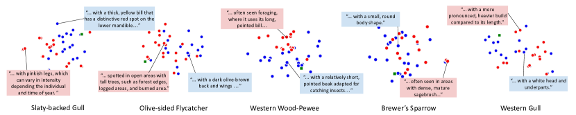
Figure 2: t-SNE Plots of Class Attributes. For each category the prototype, initial set of attributes, and the final set of attributes are shown in green, blue, and red respectively. Habitat, relative characteristics, and other distinguishing features are often identified through pairwise comparisons, while the initial attributes tend to describe the prominent visual features. These plots were obtained by mapping the CLIP text embeddings of the attributes using t-SNE. Please zoom in for details and see Appendix for a detailed figure.

Figure 2 illustrates the evolution of the attribute space across various categories. For each category, the class prototype (“photo of [class]”), the initial set of attributes, and the final set of attributes are shown in green, blue, and red, respectively. These visualizations were generated by projecting CLIP text embeddings of the attributes using t-SNE. Several new attributes were added through pairwise comparisons, and a few notable examples are highlighted in the figure. Many of the attributes discovered through pairwise comparison highlight differences in habitat, relative characteristics (e.g., “…more pronounced build compared to its length” for the Western Gull), and other distinguishing features. Bird images often include backgrounds indicative of habitat types, and this form of supervision enables CLIP to learn to associate these attributes with categorization. Larger versions of these figures are in the Appendix.

Table 5: Class Confusions. (Left) Progressive reduction of pairwise confusion between “Western Gull” and “California Gull” over training iterations of GTA-CLIP. (Right) Most confused class pairs according to our selection criteria. We show the counts of pairwise misclassified test images according to our procedure and according to a linear classifier trained on the labeled training images using the CLIP image features.

Confused Class Pairs		Ours	Linear
California Gull	Western Gull	16	10
Least Flycatcher	Olive sided Flycatcher	13	3
American Crow	Common Raven	8	12
Least Flycatcher	Western Wood Pewee	7	6
Eared Grebe	Horned Grebe	7	11
Bronzed Cowbird	Shiny Cowbird	6	3
Brewer Sparrow	Harris Sparrow	6	2
Slaty backed Gull	Western Gull	5	6
Baird Sparrow	Grasshopper Sparrow	5	3
Philadelphia Vireo	Warbling Vireo	5	8

6 Limitations

There are two main limitations to our work. The first is the use of LLMs to generate fine-grained attributes. LLMs are known to sometimes hallucinate data, and there is a risk that some attributes may be incorrect. In our initial experiments, we also found that results vary depending on the LLM used. Additionally, there is an interaction with the benchmark to which the LLM is applied; a higher-performing language model might generate lower-quality fine-grained attributes on a specific benchmark due to a pre-training data mismatch, which can lead to poorer performance with our method. The second limitation is the applicability of transductive learning. This approach is constrained by the extent of knowledge available about the query set before evaluation. In this work, we have not demonstrated robustness to imperfect knowledge of the classes and data distribution. For instance, we implicitly assume that images within a class cluster together, allowing us to model each class as a Gaussian distribution, which may not always be valid.

7 Conclusion

Despite its limitations, the transductive setting offers a compelling approach for practitioners and domain experts who need precise answers for specific datasets. For instance, an ecologist might be interested in estimating species counts from data gathered via a network of camera traps, while a scientist might want to determine land-cover distribution using satellite imagery. VLMs enable straightforward labeling through language-based descriptions of categories, but their initial accuracy is often insufficient. Our work demonstrates that expanding categories based on attributes, when combined with transductive learning, enables model fine-tuning to achieve significant accuracy improvements. Additionally, this approach offers complementary advantages to traditional labeling methods, such as providing a few labeled examples per class. While we use large language models for convenience, this iterative procedure is naturally suited to human-in-the-loop approaches, allowing practitioners to incrementally add attributes and labels for ambiguous classes. These findings are practically valuable, as they offer end-users multiple pathways to improve labeling precision on their target dataset without investing significant efforts on training dataset curation and model training.

Acknowledgments

Experiments were performed on the University of Massachusetts GPU cluster funded by the Mass. Technology Collaborative. OS and SM were supported in part by a NSF grant #2329927.

Supplementary Material

8 Additional Ablations

We explore additional ablative studies over GTA-CLIP and its various components in this section.

Table 6: Per-dataset results of Ablation Study. For five datasets on the ViT-B/16 architecture, we present the effect of various components of GTA-CLIP. We use the same conventions as Tab. 4.

Attributes	Transduct	Adapt	CUB	Cars	Aircraft	Flower	Food	Average
$\O$	✗	✗	55.20	65.38	24.75	71.38	86.10	60.56
S	✗	✗	57.70	65.65	24.78	73.33	86.50	61.59
$\O$	✓	✗	62.23	68.87	26.88	76.17	87.15	64.26
S	✓	✗	64.15	69.83	26.73	80.06	87.25	65.60
S	✓	✓	65.86	71.33	28.62	80.67	87.30	66.76
D	✓	✗	64.20	69.53	26.58	80.23	87.27	65.56
D	✓	✓	66.76	72.09	29.31	82.05	87.38	67.52

Table 7: Performance with MetaCLIP. We change the base VLM from CLIP to MetaCLIP for TransCLIP and GTA-CLIP and observe consistent improvements over the baselines on ViT-B/16

Method	CUB	Cars	Aircraft	Flower	Food	Average
CLIP	55.20	65.38	24.75	71.38	86.10	60.56
TransCLIP	62.23	68.87	26.88	76.17	87.15	64.26
GTA-CLIP	66.76	72.09	29.31	82.05	87.38	67.52
MetaCLIP	68.67	74.49	28.65	73.81	84.01	65.93
TransMetaCLIP	74.02	79.01	31.56	80.15	85.53	70.05
GTA-MetaCLIP	78.36	82.30	35.58	81.57	85.98	72.76

Table 8: Effect of LLM model on accuracy of GTA-CLIP. We switch the LLM model used by GenerateAttributes from Llama-3.1 to GPT4o and observe similar performance on ViT-B/16.

LLM	CUB	Cars	Aircraft	Flower	Food	Average
GPT4o	66.50	72.13	29.89	81.55	87.36	67.49
Llama-3.1	66.76	72.09	29.31	82.05	87.38	67.52

Table 9: Removing the internal transductive update step in GenerateAttributes, thereby making only a single call to Transduct per iteration reduces the accuracy on average over five datasets on the ViT-B/16 architecture.

LLM	CUB	Cars	Aircraft	Flower	Food	Average
GTA-CLIP single Transduct	66.72	69.89	29.55	81.32	87.32	66.96
GTA-CLIP original	66.76	72.09	29.31	82.05	87.38	67.52

Table 10: Sensitivity analysis over the top-$k$ and $T$ selection of GTA-CLIP using the CLIP ViT-B/16 architecture without the dynamic GenerateAttributes component (ie. TransCLIP^FT in Tab. 1) as given in Algorithm 1. We pick $k=8,T=30$ even though there exist better performing alternatives. We fix this hyperparameter selection to ablate on the remaining parameters of GTA-CLIP.

top-$k$	$T$	CUB [47]	Cars [17]	Aircrafts [23]	Flowers [31]	Food [5]	Average
1	30	65.93	71.55	29.43	81.04	87.36	67.06
3	30	65.64	71.97	28.95	82.01	87.43	67.20
5	30	65.64	71.97	28.74	81.28	87.39	67.00
8	30	65.86	71.33	28.62	80.67	87.30	66.76
10	30	65.84	71.45	28.53	81.04	87.43	66.86
20	30	66.09	71.97	28.29	81.04	87.36	66.95
8	1	63.98	69.87	27.48	80.76	87.37	65.89
8	10	65.05	70.55	28.17	81.04	87.36	66.43
8	20	65.48	71.11	28.47	81.04	87.43	66.71
8	30	65.86	71.33	28.62	80.67	87.30	66.76
8	40	66.14	72.63	28.80	81.04	87.34	67.19
8	50	66.14	72.71	28.98	82.01	87.43	67.46

Table 11: Ablation over the probability threshold $\alpha$ of the GenerateAttributes implementation of GTA-CLIP as given in Sec. 4 using $k=8,T=30$ as determiend from Tab. 10. Like Tab. 10, even though there are better performing selection, we choose $\alpha=10\%$.

$\alpha$	CUB [47]	Cars [17]	Aircrafts [23]	Flowers [31]	Food [5]	Average
2.5%	65.67	71.68	28.50	83.23	87.27	67.27
5.0%	66.69	71.67	28.50	81.04	87.40	67.06
7.5%	66.98	71.56	28.98	80.67	87.32	67.10
10.0%	66.76	72.09	29.31	82.05	87.38	67.52
12.5%	65.48	72.64	28.47	82.01	87.50	67.22
15.0%	66.90	71.74	28.65	82.05	87.41	67.35
17.5%	66.83	72.65	28.83	82.42	87.29	67.61
20.0%	66.72	72.99	28.95	80.88	87.33	67.37

Per Dataset Results.

Tab. 6 breaks down the Top-1 accuracies across reported in Tab. 4 of the main papers across individual datasets namely CUB, Stanford Cars, FGVC Aircraft, Flowers102, and Food101 datasets using the ViT-B/16 architecture. We observe similar trends for each dataset for all the ablations considered.

Using MetaCLIP as the base VLM.

MetaCLIP introduces better CLIP architectures by curating training data and scaling training. We switch the base VLM from CLIP to MetaCLIP to take advantage of this and test the generalization of our approach to new architectures. Tab. 7 presents the accuracies for the inductive version of MetaCLIP, TransMetaCLIP (the TransCLIP method applied to MetaCLIP), and GTA-MetaCLIP (our method applied to MetaCLIP). The experiments are conducted using the ViT-B/16 architecture of MetaCLIP across CUB, Stanford Cars, FGVC Aircraft, Flowers102, and Food101 datasets. We observe consistent improvements in the case of MetaCLIP too. On average, over the five datasets, we see an improvement of 6.8% over MetaCLIP, and an improvement of 2.7% over TransMetaCLIP on using our method. This is similar to our improvements of 7.0% and 3.3% on the corresponding baselines with CLIP.

Effect of the LLM Model in GenerateAttributes.

For all the results in the main paper, we used Llama-3.1 as the LLM model for dynamic attribute generation. Now we explore using GPT4o as the LLM in Tab. 8. We observe that the accuracy remains similar on average over the CUB, Stanford Cars, FGVC Aircraft, Flowers102, and Food101 datasets on ViT-B/16. Thus, using Llama-3.1 is a more cost-effective choice for dynamic attribute generation due to its open-source nature.

Removing the internal call to Transduct in GenerateAttributes. We remove the internal transductive inference update call (see § 3.2) in GenerateAttributes and present the results over five datasets using the ViT-B/16 architecture in Tab. 9. We observe that on average the accuracy drops on removing this call to Transduct. For Aircraft, we observe that the accuracy slightly improves on dropping this Transduct call, however for Cars we see a significant decrease.

9 Sensitivity Analysis

Top-$k$ Selection and Number of Iterations $T$.

In Tab. 10 we show the performance of GTA-CLIP when varying top-$k$ and $T$ selection. The table is divided into two sections: first we fix $T$ and sweep over $k$, and secondly we fix $k$ and sweep over $T$. We find that increasing $T$ has the strongest correlation with performance, with average performance across benchmarks monotonically increasing for $k=8$ when going from $T=1$ to $T=50$. Furthermore, we find that Flowers and Food are the most insensitive to changes in hyperparameters, keeping mostly the same value irrespective of $k$ and $T$. Overall, we find the performance guarantees to be quite high even in the worst case ($65.89$ with $k=8,T=1$), still being higher than default TransCLIP ($64.26$) or TransCLIP with static fine-grained attributes ($65.60$).

Probability Threshold $\alpha$.

Similarly, in Tab. 11 we show the performance of GTA-CLIP when varying the probability threshold for determining confusing pairs of classes, $\alpha$. For the whole experiment, we fix $k=8,T=30$ and sweep over $alpha$. We find that each benchmark has it’s own ideal $\alpha$ value, namely that no two benchmark’s max performances share an common $alpha$. Surprisingly, we see that $\alpha=17.5\%$, which does not perform the best on any benchmark, has the highest average value. We also conclude that GTA-CLIP has a greater insensitivity to the choice of $\alpha$ as compared to $T$ but similar to $k$. Namely we find that the spread of $\alpha$ to be $67.61-67.06=0.55$, $T$ to be $67.46-65.89=1.57$, and $k$ to be $67.20-66.76=0.44$. Finally, we find that the minimum performance increase by introducing GenerateAttributes is at $\alpha=5.0\%$ with a gain of $67.10-66.76=0.34$. In other words, adding any amount of comparative attribute generation improves performance.

10 Evolution of Attribute Space

In Fig. 3 through Fig. 7, we depict the evolution of the set of attributes for a given class over the course of our method. GTA-CLIP begins with a list of static fine-grained attributes (depicted in blue) and through iterations of the method generates additional comparative attributes between confusing classes (red). We embed these attributes with the CLIP text tower and use t-SNE to visualize the relative locations of these attributes. The specific prompt generated for a given point is indicated within the figure. We see that attributes within the reduced space often form tight clusters grouped by similar concepts (eg. ”habitat” or ”appearance”). When dynamically generated attributes (red points) are close to the initial static attributes (blue) we see more similar semantic meaning. Finally, one can notice that the newly added attributes occupy different regions of the space, namely that using dynamic generation effectively expands the list of fine-grained details on a given class.

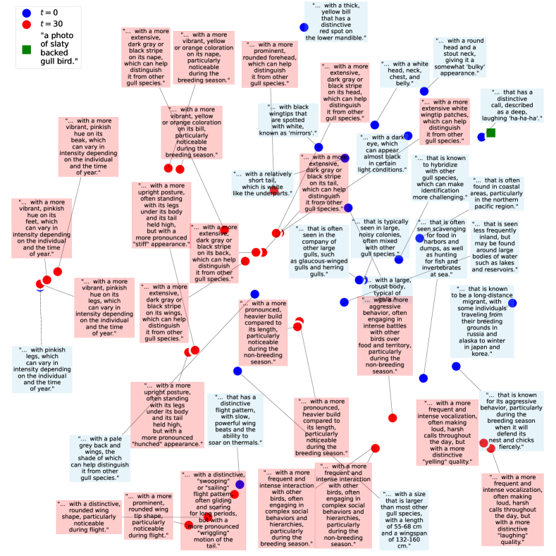
Figure 3: Slaty-backed Gull (vs. Western Gull) Annotated T-SNE Plot.

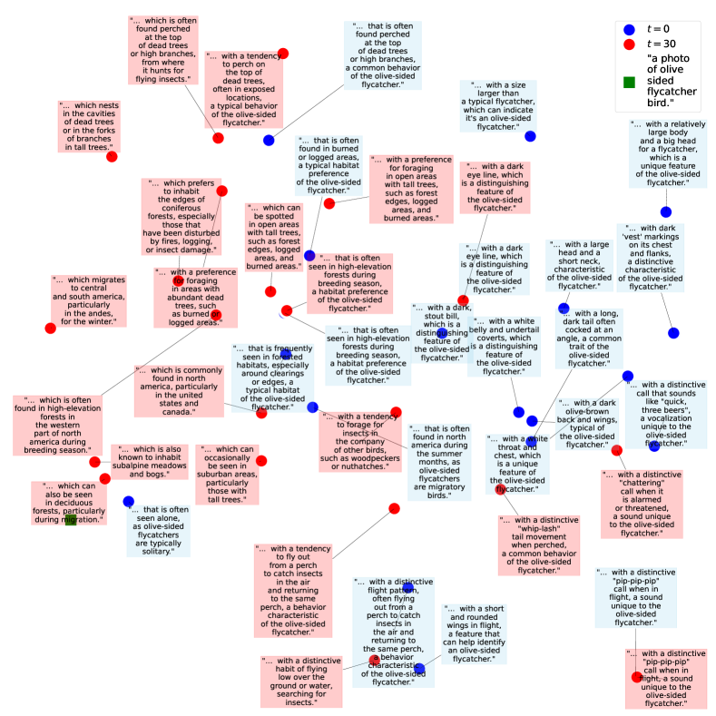
Figure 4: Olive-sided Flycatcher (vs. Least Flycatcher) Annotated t-SNE Plot.

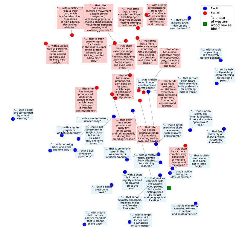
Figure 5: Western Wood-Pewee (vs. Least Flycatcher) Annotated t-SNE Plot.

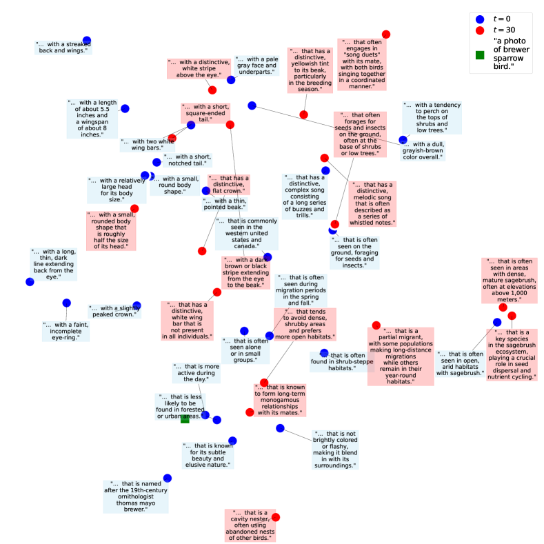
Figure 6: Brewer’s Sparrow (vs. Harris’ Sparrow) Annotated t-SNE Plot.

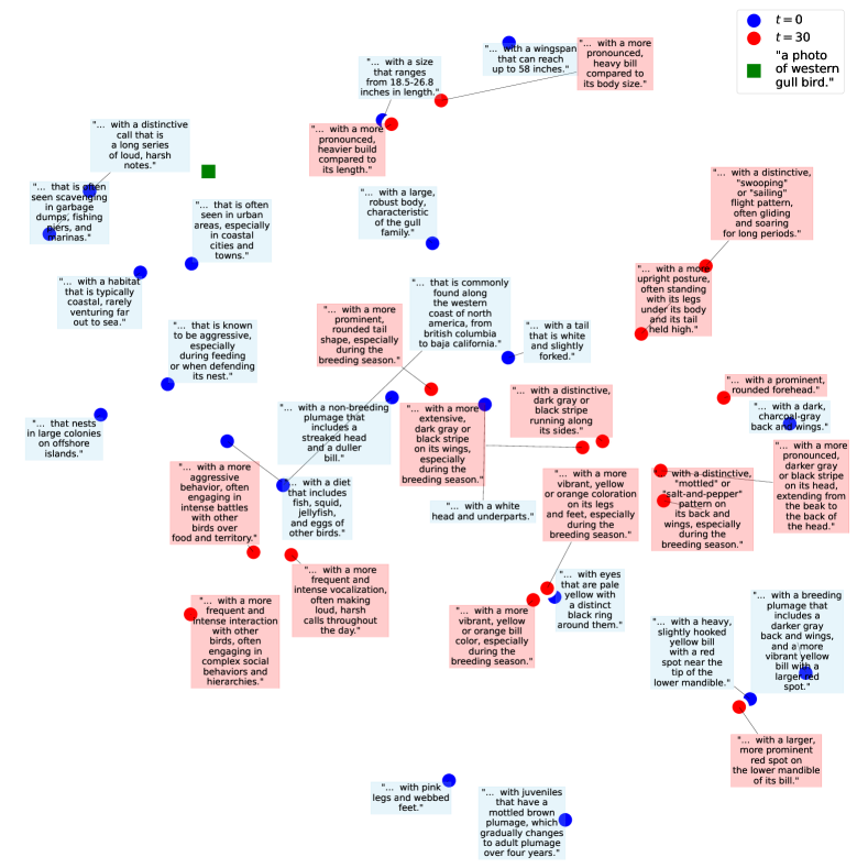
Figure 7: Western Gull (vs. California Gull) Annotated t-SNE Plot.

References

- [1] Josh Achiam, Steven Adler, Sandhini Agarwal, Lama Ahmad, Ilge Akkaya, Florencia Leoni Aleman, Diogo Almeida, Janko Altenschmidt, Sam Altman, Shyamal Anadkat, et al. Gpt-4 technical report. arXiv preprint arXiv:2303.08774, 2023.
- [2] Rie Ando and Tong Zhang. Learning on graph with laplacian regularization. Advances in neural information processing systems, 19, 2006.
- [3] Eric Arazo, Diego Ortego, Paul Albert, Noel E O’Connor, and Kevin McGuinness. Pseudo-labeling and confirmation bias in deep semi-supervised learning. In 2020 International joint conference on neural networks (IJCNN), pages 1–8. IEEE, 2020.
- [4] Liu Bo, Qiulei Dong, and Zhanyi Hu. Hardness sampling for self-training based transductive zero-shot learning. In Proceedings of the IEEE/CVF Conference on Computer Vision and Pattern Recognition, pages 16499–16508, 2021.
- [5] Lukas Bossard, Matthieu Guillaumin, and Luc Van Gool. Food-101–mining discriminative components with random forests. In Computer vision–ECCV 2014: 13th European conference, zurich, Switzerland, September 6-12, 2014, proceedings, part VI 13, pages 446–461. Springer, 2014.
- [6] Paola Cascante-Bonilla, Fuwen Tan, Yanjun Qi, and Vicente Ordonez. Curriculum labeling: Revisiting pseudo-labeling for semi-supervised learning. In Proceedings of the AAAI conference on artificial intelligence, volume 35, pages 6912–6920, 2021.
- [7] Mia Chiquier, Utkarsh Mall, and Carl Vondrick. Evolving interpretable visual classifiers with large language models. arXiv preprint arXiv:2404.09941, 2024.
- [8] Mircea Cimpoi, Subhransu Maji, Iasonas Kokkinos, Sammy Mohamed, and Andrea Vedaldi. Describing textures in the wild. In Proceedings of the IEEE conference on computer vision and pattern recognition, pages 3606–3613, 2014.
- [9] Li Fei-Fei, Rob Fergus, and Pietro Perona. Learning generative visual models from few training examples: An incremental bayesian approach tested on 101 object categories. In 2004 conference on computer vision and pattern recognition workshop, pages 178–178. IEEE, 2004.
- [10] Yanwei Fu, Timothy M Hospedales, Tao Xiang, and Shaogang Gong. Transductive multi-view zero-shot learning. IEEE transactions on pattern analysis and machine intelligence, 37(11):2332–2345, 2015.
- [11] Peng Gao, Shijie Geng, Renrui Zhang, Teli Ma, Rongyao Fang, Yongfeng Zhang, Hongsheng Li, and Yu Qiao. Clip-adapter: Better vision-language models with feature adapters. International Journal of Computer Vision, 132(2):581–595, 2024.
- [12] Rui Gao, Xingsong Hou, Jie Qin, Jiaxin Chen, Li Liu, Fan Zhu, Zhao Zhang, and Ling Shao. Zero-vae-gan: Generating unseen features for generalized and transductive zero-shot learning. IEEE Transactions on Image Processing, 29:3665–3680, 2020.
- [13] Yves Grandvalet and Yoshua Bengio. Semi-supervised learning by entropy minimization. Advances in neural information processing systems, 17, 2004.
- [14] Patrick Helber, Benjamin Bischke, Andreas Dengel, and Damian Borth. Eurosat: A novel dataset and deep learning benchmark for land use and land cover classification. IEEE Journal of Selected Topics in Applied Earth Observations and Remote Sensing, 12(7):2217–2226, 2019.
- [15] Mingyi Hong, Xiangfeng Wang, Meisam Razaviyayn, and Zhi-Quan Luo. Iteration complexity analysis of block coordinate descent methods. Mathematical Programming, 163:85–114, 2017.
- [16] Yannis Kalantidis, Giorgos Tolias, et al. Label propagation for zero-shot classification with vision-language models. In Proceedings of the IEEE/CVF Conference on Computer Vision and Pattern Recognition, pages 23209–23218, 2024.
- [17] Jonathan Krause, Michael Stark, Jia Deng, and Li Fei-Fei. 3d object representations for fine-grained categorization. In Proceedings of the IEEE international conference on computer vision workshops, pages 554–561, 2013.
- [18] Kathleen M Lewis, Emily Mu, Adrian V Dalca, and John Guttag. Gist: Generating image-specific text for fine-grained object classification. arXiv e-prints, pages arXiv–2307, 2023.
- [19] Bo Liu, Lihua Hu, Qiulei Dong, and Zhanyi Hu. An iterative co-training transductive framework for zero shot learning. IEEE Transactions on Image Processing, 30:6943–6956, 2021.
- [20] Timo Lüddecke and Alexander Ecker. Image segmentation using text and image prompts. In Proceedings of the IEEE/CVF conference on computer vision and pattern recognition, pages 7086–7096, 2022.
- [21] Huaishao Luo, Junwei Bao, Youzheng Wu, Xiaodong He, and Tianrui Li. Segclip: Patch aggregation with learnable centers for open-vocabulary semantic segmentation. In International Conference on Machine Learning, pages 23033–23044. PMLR, 2023.
- [22] Subhransu Maji. Discovering a lexicon of parts and attributes. In Computer Vision–ECCV 2012. Workshops and Demonstrations: Florence, Italy, October 7-13, 2012, Proceedings, Part III 12, pages 21–30. Springer, 2012.
- [23] Subhransu Maji, Esa Rahtu, Juho Kannala, Matthew Blaschko, and Andrea Vedaldi. Fine-grained visual classification of aircraft. arXiv preprint arXiv:1306.5151, 2013.
- [24] Mayug Maniparambil, Chris Vorster, Derek Molloy, Noel Murphy, Kevin McGuinness, and Noel E O’Connor. Enhancing clip with gpt-4: Harnessing visual descriptions as prompts. In Proceedings of the IEEE/CVF International Conference on Computer Vision, pages 262–271, 2023.
- [25] Ségolène Martin, Yunshi Huang, Fereshteh Shakeri, Jean-Christophe Pesquet, and Ismail Ben Ayed. Transductive zero-shot and few-shot clip. In Proceedings of the IEEE/CVF Conference on Computer Vision and Pattern Recognition, pages 28816–28826, 2024.
- [26] Sachit Menon and Carl Vondrick. Visual classification via description from large language models. In The Eleventh International Conference on Learning Representations.
- [27] Matthias Minderer, Alexey Gritsenko, and Neil Houlsby. Scaling open-vocabulary object detection. Advances in Neural Information Processing Systems, 36, 2024.
- [28] Muhammad Jehanzeb Mirza, Leonid Karlinsky, Wei Lin, Horst Possegger, Mateusz Kozinski, Rogerio Feris, and Horst Bischof. Lafter: Label-free tuning of zero-shot classifier using language and unlabeled image collections. Advances in Neural Information Processing Systems, 36, 2024.
- [29] Muhammad Ferjad Naeem, Muhammad Gul Zain Ali Khan, Yongqin Xian, Muhammad Zeshan Afzal, Didier Stricker, Luc Van Gool, and Federico Tombari. I2mvformer: Large language model generated multi-view document supervision for zero-shot image classification. In Proceedings of the IEEE/CVF Conference on Computer Vision and Pattern Recognition, pages 15169–15179, 2023.
- [30] Andrew Ng, Michael Jordan, and Yair Weiss. On spectral clustering: Analysis and an algorithm. Advances in neural information processing systems, 14, 2001.
- [31] Maria-Elena Nilsback and Andrew Zisserman. Automated flower classification over a large number of classes. In 2008 Sixth Indian conference on computer vision, graphics & image processing, pages 722–729. IEEE, 2008.
- [32] Devi Parikh and Kristen Grauman. Interactively building a discriminative vocabulary of nameable attributes. In CVPR 2011, pages 1681–1688. IEEE, 2011.
- [33] Omkar M Parkhi, Andrea Vedaldi, Andrew Zisserman, and CV Jawahar. Cats and dogs. In 2012 IEEE conference on computer vision and pattern recognition, pages 3498–3505. IEEE, 2012.
- [34] Genevieve Patterson and James Hays. Sun attribute database: Discovering, annotating, and recognizing scene attributes. In 2012 IEEE conference on computer vision and pattern recognition, pages 2751–2758. IEEE, 2012.
- [35] Sarah Pratt, Ian Covert, Rosanne Liu, and Ali Farhadi. What does a platypus look like? generating customized prompts for zero-shot image classification. In Proceedings of the IEEE/CVF International Conference on Computer Vision, pages 15691–15701, 2023.
- [36] Alec Radford, Jong Wook Kim, Chris Hallacy, Aditya Ramesh, Gabriel Goh, Sandhini Agarwal, Girish Sastry, Amanda Askell, Pamela Mishkin, Jack Clark, et al. Learning transferable visual models from natural language supervision. In International conference on machine learning, pages 8748–8763. PMLR, 2021.
- [37] Yongming Rao, Wenliang Zhao, Guangyi Chen, Yansong Tang, Zheng Zhu, Guan Huang, Jie Zhou, and Jiwen Lu. Denseclip: Language-guided dense prediction with context-aware prompting. In Proceedings of the IEEE/CVF conference on computer vision and pattern recognition, pages 18082–18091, 2022.
- [38] Meisam Razaviyayn, Mingyi Hong, and Zhi-Quan Luo. A unified convergence analysis of block successive minimization methods for nonsmooth optimization. SIAM Journal on Optimization, 23(2):1126–1153, 2013.
- [39] Olga Russakovsky, Jia Deng, Hao Su, Jonathan Krause, Sanjeev Satheesh, Sean Ma, Zhiheng Huang, Andrej Karpathy, Aditya Khosla, Michael Bernstein, et al. Imagenet large scale visual recognition challenge. International journal of computer vision, 115:211–252, 2015.
- [40] Oindrila Saha, Grant Van Horn, and Subhransu Maji. Improved zero-shot classification by adapting vlms with text descriptions. In Proceedings of the IEEE/CVF Conference on Computer Vision and Pattern Recognition, pages 17542–17552, 2024.
- [41] Jianbo Shi and Jitendra Malik. Normalized cuts and image segmentation. IEEE Transactions on pattern analysis and machine intelligence, 22(8):888–905, 2000.
- [42] Mainak Singha, Harsh Pal, Ankit Jha, and Biplab Banerjee. Ad-clip: Adapting domains in prompt space using clip. In Proceedings of the IEEE/CVF International Conference on Computer Vision, pages 4355–4364, 2023.
- [43] K Soomro. Ucf101: A dataset of 101 human actions classes from videos in the wild. arXiv preprint arXiv:1212.0402, 2012.
- [44] Changyao Tian, Wenhai Wang, Xizhou Zhu, Jifeng Dai, and Yu Qiao. Vl-ltr: Learning class-wise visual-linguistic representation for long-tailed visual recognition. In European conference on computer vision, pages 73–91. Springer, 2022.
- [45] Hugo Touvron, Thibaut Lavril, Gautier Izacard, Xavier Martinet, Marie-Anne Lachaux, Timothée Lacroix, Baptiste Rozière, Naman Goyal, Eric Hambro, Faisal Azhar, et al. Llama: Open and efficient foundation language models. arXiv preprint arXiv:2302.13971, 2023.
- [46] Vladimir Vapnik. The support vector method of function estimation. In Nonlinear modeling: Advanced black-box techniques, pages 55–85. Springer, 1998.
- [47] Catherine Wah, Steve Branson, Peter Welinder, Pietro Perona, and Serge Belongie. The caltech-ucsd birds-200-2011 dataset. 2011.
- [48] Ziyu Wan, Dongdong Chen, Yan Li, Xingguang Yan, Junge Zhang, Yizhou Yu, and Jing Liao. Transductive zero-shot learning with visual structure constraint. Advances in neural information processing systems, 32, 2019.
- [49] Wenlin Wang, Yunchen Pu, Vinay Verma, Kai Fan, Yizhe Zhang, Changyou Chen, Piyush Rai, and Lawrence Carin. Zero-shot learning via class-conditioned deep generative models. In Proceedings of the AAAI conference on artificial intelligence, volume 32, 2018.
- [50] Wenlin Wang, Hongteng Xu, Guoyin Wang, Wenqi Wang, and Lawrence Carin. Zero-shot recognition via optimal transport. In Proceedings of the IEEE/CVF Winter Conference on Applications of Computer Vision, pages 3471–3481, 2021.
- [51] Mitchell Wortsman, Gabriel Ilharco, Jong Wook Kim, Mike Li, Simon Kornblith, Rebecca Roelofs, Raphael Gontijo Lopes, Hannaneh Hajishirzi, Ali Farhadi, Hongseok Namkoong, et al. Robust fine-tuning of zero-shot models. In Proceedings of the IEEE/CVF conference on computer vision and pattern recognition, pages 7959–7971, 2022.
- [52] Jianxiong Xiao, James Hays, Krista A Ehinger, Aude Oliva, and Antonio Torralba. Sun database: Large-scale scene recognition from abbey to zoo. In 2010 IEEE computer society conference on computer vision and pattern recognition, pages 3485–3492. IEEE, 2010.
- [53] Qizhe Xie, Minh-Thang Luong, Eduard Hovy, and Quoc V Le. Self-training with noisy student improves imagenet classification. In Proceedings of the IEEE/CVF conference on computer vision and pattern recognition, pages 10687–10698, 2020.
- [54] Mengde Xu, Zheng Zhang, Fangyun Wei, Yutong Lin, Yue Cao, Han Hu, and Xiang Bai. A simple baseline for open-vocabulary semantic segmentation with pre-trained vision-language model. In European Conference on Computer Vision, pages 736–753. Springer, 2022.
- [55] Xun Xu, Timothy Hospedales, and Shaogang Gong. Transductive zero-shot action recognition by word-vector embedding. International Journal of Computer Vision, 123:309–333, 2017.
- [56] I Zeki Yalniz, Hervé Jégou, Kan Chen, Manohar Paluri, and Dhruv Mahajan. Billion-scale semi-supervised learning for image classification. arXiv preprint arXiv:1905.00546, 2019.
- [57] An Yan, Yu Wang, Yiwu Zhong, Chengyu Dong, Zexue He, Yujie Lu, William Yang Wang, Jingbo Shang, and Julian McAuley. Learning concise and descriptive attributes for visual recognition. In Proceedings of the IEEE/CVF International Conference on Computer Vision, pages 3090–3100, 2023.
- [58] Xiangli Yang, Zixing Song, Irwin King, and Zenglin Xu. A survey on deep semi-supervised learning. IEEE Transactions on Knowledge and Data Engineering, 35(9):8934–8954, 2022.
- [59] Yunlong Yu, Zhong Ji, Jichang Guo, and Yanwei Pang. Transductive zero-shot learning with adaptive structural embedding. IEEE transactions on neural networks and learning systems, 29(9):4116–4127, 2017.
- [60] Yunlong Yu, Zhong Ji, Xi Li, Jichang Guo, Zhongfei Zhang, Haibin Ling, and Fei Wu. Transductive zero-shot learning with a self-training dictionary approach. IEEE transactions on cybernetics, 48(10):2908–2919, 2018.
- [61] Maxime Zanella, Benoît Gérin, and Ismail Ben Ayed. Boosting vision-language models with transduction. In Neural Information Processing Systems (NeurIPS), 2024.
- [62] Bowen Zhang, Yidong Wang, Wenxin Hou, Hao Wu, Jindong Wang, Manabu Okumura, and Takahiro Shinozaki. Flexmatch: Boosting semi-supervised learning with curriculum pseudo labeling. Advances in Neural Information Processing Systems, 34:18408–18419, 2021.
- [63] Renrui Zhang, Rongyao Fang, Wei Zhang, Peng Gao, Kunchang Li, Jifeng Dai, Yu Qiao, and Hongsheng Li. Tip-adapter: Training-free clip-adapter for better vision-language modeling. arXiv preprint arXiv:2111.03930, 2021.
- [64] Xin Zhang, Shixiang Shane Gu, Yutaka Matsuo, and Yusuke Iwasawa. Domain prompt learning for efficiently adapting clip to unseen domains. Transactions of the Japanese Society for Artificial Intelligence, 38(6):B–MC2_1, 2023.
- [65] Yiwu Zhong, Jianwei Yang, Pengchuan Zhang, Chunyuan Li, Noel Codella, Liunian Harold Li, Luowei Zhou, Xiyang Dai, Lu Yuan, Yin Li, et al. Regionclip: Region-based language-image pretraining. In Proceedings of the IEEE/CVF conference on computer vision and pattern recognition, pages 16793–16803, 2022.
- [66] Kaiyang Zhou, Jingkang Yang, Chen Change Loy, and Ziwei Liu. Conditional prompt learning for vision-language models. In Proceedings of the IEEE/CVF conference on computer vision and pattern recognition, pages 16816–16825, 2022.
- [67] Kaiyang Zhou, Jingkang Yang, Chen Change Loy, and Ziwei Liu. Learning to prompt for vision-language models. International Journal of Computer Vision, 130(9):2337–2348, 2022.