Author preprint January 2025
Resiliency metrics quantifying emergency response in a distribution system

Abstract

The electric distribution system is a cornerstone of modern life, playing a critical role in the daily activities and well-being of individuals. As the world transitions toward a decarbonized future, where even mobility relies on electricity, ensuring the resilience of the grid becomes paramount. This paper introduces novel resilience metrics designed to equip utilities and stakeholders with actionable tools to assess performance during storm events. The metrics focus on emergency storm response and the resources required to improve customer service. The practical calculation of the metrics from historical utility data is demonstrated for multiple storm events. Additionally, the metrics’ improvement with added crews is estimated by “rerunning history” with faster restoration. By applying this resilience framework, utilities can enhance their restoration strategies and unlock potential cost savings, benefiting both providers and customers in an era of heightened energy dependency.

I Introduction

Distribution system resilience can be divided into two key categories: system resilience and operational resilience. System resilience refers to the ability of the distribution grid to withstand extreme weather events while continuing to serve customers. Operational resilience, on the other hand, is a quantification of the restoration efforts, including resource deployment, grid automation performance, and the efficiency of the resources used to restore service to customers. Metrics that can assess both these categories are important to understand overall distribution system resilience.

In existing literature, resilience metrics often focus heavily on the restoration of critical loads, such as hospitals and police stations. While restoring these essential services remains a priority, this paper introduces operational metrics aimed at optimizing the restoration of all loads, ensuring an effective and efficient recovery process across the entire grid.

When the distribution grid encounters extreme weather and experiences outages, the restoration process is immediately activated. In anticipation of impending extreme weather events, utilities assess their potential impact and pre-position resources. This proactive approach is crucial, as mobilizing resources can be time-consuming and may leave customers without power for extended periods. The speed and effectiveness (while putting safety of crews and customers as the top priority) with which human resources restore power after an outage is a key indicator of organizational resilience, and their performance should be systematically monitored and compared to previous events. However, there is currently no widely adopted metric for this purpose. The metrics describing emergency response need to be simple to promote adoption among utilities.

Grid automation technologies, such as feeder reconfiguration, customer restoration through alternative sources (like alternate feeders), sectionalization, energy storage systems, emergency resources, or microgrids, can also play a pivotal role in the restoration process [1]-[2]. Additionally, a metric that tracks customer restoration progress during an event, and compares it to pre-established targets based on historical performance, can provide valuable insights into the progress and efficiency of restoration efforts. By monitoring the achievement of these targets across multiple events, utilities can assess their annual performance, identifying areas of improvement where restoration goals were not met.

It is crucial to understand the distribution utility restoration process [3]. As shown in Fig. 1, a team of dispatchers in the control center monitors the Outage Management System (OMS) as outages occur and are restored. Based on this, they assign tickets to field crews, dispatching them to repair outages and restore service to customers. This process remains manual at its final stage, relying on phone communication between dispatchers and crews. At times, incorrect crews may be sent if the situation is not fully understood.

For example, if an outage is caused by vegetation, such as a tree bringing down a power line, the proper sequence involves sending a wire watcher first to monitor the situation, followed by a tree crew to clear the obstruction, and finally a construction crew to repair the line. However, if the patrol is insufficient or patrolling resources are lacking, a construction crew might be dispatched prematurely, leading to wasted time and labor with no progress made on the repair.

We briefly indicate previous work calculating distribution system resilience metrics from observed data. Wei and Ji [4] analyze distribution system resilience with data from hurricane Ike with a non-homogeneous Poisson outage process arriving at a queue that repairs the outages to produce a dynamically varying restore process. Carrington [5] systematically extracts outage and restore processes and performance curves and their metrics from events in detailed utility outage data. Kandaperumal [6] develops metrics describing the threats, network topology, generation, loads, and restoration, and uses data from an Alaskan town to show how the metrics can be used to improve resilience planning and operation. Using EAGLE-I data scraped from web outage reports, Ericson [7] extracts performance curves and frequency and duration statistics and Abdelmalak [8] extracts the distributions of resilience metrics for extreme events that cross thresholds in the number of customers out. Ahmad [10] extracts baseline resilience metrics from detailed utility outage data, and introduces the rerunning history method to quantify the benefits of the overall effects of better restoration or hardening the grid for wind.

In this paper, we describe the challenges of emergency response and leverage and advance beyond [5, 10] to define and extract new restoration metrics from utility data, including new metrics that describe crew performance, a topic that has been neglected in previous work.

Figure 1: Crew Dispatching Hierarchy

II Emergency Response Effectiveness

The efficiency and speed of emergency response after an extreme event depend primarily on the severity and trajectory of the extreme weather event. The process can, however be improved through proactive measures such as deploying crews to heavily impacted areas and optimizing restoration efforts. Prior to the event, utilities strategically allocate crews for restoration based on the event forecast and preliminary assessment. As the event unfolds, this assessment is continuously updated by closely monitoring its impact, allowing for the allocation of crews to the most heavily affected areas. Once the event has passed, the restoration process can be fine-tuned to maximize the number of customers restored in the shortest possible time.

Given the severe and sometimes sudden nature of high-impact events, even the best efforts in crew scheduling may not be optimal. Crew managers respond to outage reports through their outage reporting and management systems, prioritizing those with the highest customer counts for immediate dispatch of resources. While consideration is given to critical customers, the primary focus is on addressing high customer outage scenarios. The effectiveness of proactive crew allocation hinges significantly on the accuracy of event forecasts. Inaccurate forecasts may necessitate the mobilization of additional contractor crews and the solicitation of mutual assistance from other utilities.

Restoration crews often face travel challenges, extensive road damage, and hazardous environments, making crew safety paramount. Repair tasks can range from simple fuse replacements to complex multi-span pole replacements. Supply chain issues may further complicate the process if materials are not readily available. Additionally, the extent of damage does not always correlate with the number of customer interruptions, especially in rural or developing areas with long tap feeders serving few customers. Therefore, meticulous assessment and planning are essential for effective crew scheduling and resource allocation.

During an event, the distribution system operator typically dispatches crews to outages in chronological order. While scheduling chronologically is common, prioritizing outages with many customers, critical loads, and minimizing crew travel time is more effective. Emergency response efficiency hinges on crew allocation and repair scheduling. A metric to capture this efficiency from start to finish should be easily derived from available data and provide consistent, actionable insights. The metric should also be flexible to incorporate utility specific actions while being capable of widespread adoption.

III Extracting events & metrics from utility data

Utilities can readily process the outage data related to particular extreme weather events from their outage management system logs to capture the various processes that inform the operational resilience metrics. The accumulated customer outages form the outage process $O(t)$ and the accumulated restored customers form the restore process $R(t)$ as time $t$ increases. The performance curve $P(t)$ is the accumulated number of unrestored customers. The area under the performance curve is equivalent to the area between the outage process and the restore process, which is quantified as the customer hours metric, ($A^{\text{cust}}$). Along with the crew deployment on the system by the hour during the event, Fig. 2 visualize the operational resilience processes.

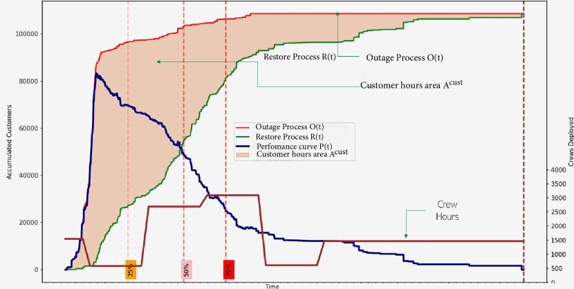
Figure 2: Operational resilience processes

Since operation resiliency analysis assesses system performance based on events, individual outages are grouped per extreme weather event. Since simultaneous outages occur when the grid is stressed, the grouping can be done by detecting the outages that overlap (that is, the outages that occur before all the previous outages are restored) to form the event [5]. The number of outages in an event ($n$) is a measure of the grid’s strength relative to the storm intensity. The start time of an event $o_{1}$ is defined by an initial outage that occurs when all system components are operational, and the end of the same event is defined by the first subsequent time $r_{n}$ when all the components are restored. We write $o_{1}\leq o_{2}\leq\cdots\leq o_{n}$ for the outage times in the order in which they occur and $r_{1}\leq r_{2}\leq\cdots\leq r_{n}$ for the restore times in the order in which they occur. The outages happen in the time interval $[o_{1},o_{n}]$ and the restores happen in the time interval $[r_{1},r_{n}]$. In real outage data, the restores typically start before the outages end, so that these time intervals overlap.

We write $c_{k}$ for the number of customers outaged at the $k$th outage. The total number of customers outaged during the event is $n^{\rm cust}=c_{1}+c_{2}+\cdots+c_{n}$. $n^{\rm cust}$ and $n$ are useful metrics describing the size of the event in terms of customer impact and utility impact respectively.

We form the curve of the customer outage process $O^{\rm cust}(t)$, which is the accumulated number of customers outaged at time $t$ during the event. And we form the curve of the customer restore process $R^{\rm cust}(t)$, which is the accumulated number of customers restored at time $t$ during the event:

$$O^{\rm cust}(t)=\sum_{o_{k}\leq t}c_{k}~\mbox{ and }~R^{\rm cust}(t)=\sum_{r_{k}\leq t}c_{k}$$ (1)

As shown in Fig. 2, the customer outage process $O^{\rm cust}(t)$ starts from zero at the beginning of the event and rises to the total number of customers out $n^{\rm cust}$ during the event. The customer restore process $R^{\rm cust}(t)$ starts from zero shortly after the beginning of the event and rises to $n^{\rm cust}$ at the end of the event. The customer restore process in effect tries to catch up with the customer outage process and the event ends when it does catch up and all the customers are restored.

The customer performance curve $P^{\rm cust}(t)$ tracks the accumulated number of unrestored customers at time $t$ during the event as shown in Fig. 2. We have the relationship:

$$P^{\rm cust}(t)=O^{\rm cust}(t)-R^{\rm cust}(t).$$ (2)

This follows since the unrestored outages increase when customers are outaged and deccrease when the customers are restored. (Often $P^{\rm cust}(t)$ is plotted below the time axis and then it changes sign so that it is $R^{\rm cust}(t)-O^{\rm cust}(t)$ [5, 11, 10].)

Instead of tracking the number of customers outaged or restored, we can similarly track the number of outages to obtain the outage process $O(t)$, which is the accumulated number of outages at time $t$ during the event, the restore process $R(t)$, which is the accumulated number of restores at time $t$, and the performance curve $P(t)=O(t)-R(t)$, which is the accumulated number of unrestored outages at time $t$.

Many useful metrics now follow from the dimensions and areas of the outage and restore processes. The metrics are summarized in Table I, including an example of their values for a particular storm. It is useful to divide the metrics into those describing the outage process and the strength of the grid relative to the storm, those describing the restore process and the recovery, and those describing the performance curve and the combined effect of the outage and restore processes.

Customer hours $A^{\rm cust}$: Perhaps the most useful metric assessing the impact of the event on the customers is the total customer hours out $A^{\rm cust}$. $A^{\rm cust}$ combines the event size in terms of number of customers with duration. It turns out [11] that $A^{\rm cust}$ is also the area between the performance curve $P^{\rm cust}$ and the time axis and also the area between the outage process $O^{\rm cust}(t)$ and the restore process $R^{\rm cust}(t)$. We write $d_{k}$ for the duration of the $k$th outage. Then two ways to calculate $A^{\rm cust}$ are

$$A^{\rm cust} =\sum_{k=1}^{n}c_{k}d_{k}=\int_{o_{1}}^{r_{n}}|P^{\rm cust}(t)|dt$$ (3)

Note that the $A^{\rm cust}$ is the contribution of the outages in the event towards the numerator of SAIDI if the event is not excluded from SAIDI as a major event day. The resilience metric $A^{\rm cust}$ measures the customer hours lost in an event or class of events whereas SAIDI measures outages over the year.

TABLE I: Resilience Metrics for an Event

OUTAGE PROCESS METRICS
number of outages	$n$	850
number of customers out	$n^{\rm cust}$	88923
outage duration (storm duration)	$o_{n}-o_{1}$	29
outage rate	$n/(o_{n}-o_{1})$	29.31
RESTORE PROCESS METRICS
delay before start of restore	$r_{1}-o_{1}$	0.567
restore duration	$r_{n}-r_{1}$	70
duration to 95% restore	$D^{\rm restore}_{95\%}$	49
customer restore rate	$n^{\rm cust}/(r_{n}-r_{1})$	1270.3
outage restore rate	$n/(r_{n}-r_{1})$	12.14
crew hours for restoration	$C^{\rm crew}$	72264
Restoration Efficiency RE	$\log_{10}[C^{\rm crew}/n]$	1.948
PERFORMANCE CURVE METRICS
event duration	$r_{n}-o_{1}$	9
max customers simultaneously out	$\max_{t}|P^{\rm cust}(t)|$	32959
max number simultaneous outages	$\max_{t}|P(t)|$	501
customer hours out and $P(t)$ area	$A^{\rm cust}$	753380
Area Index of Resilience AIR	$\log_{10}[A^{\rm cust}/n^{\rm cust}]$	0.928
REPAIR = RE Plus AIR	RE + AIR	2.876

Crew hours $C^{\rm crew}$: One way to track the restoration effort of the utility is by the number of crews, measured by full time equivalents (FTEs). The curve $C(t)$ is the number of crews deployed at time $t$. $C(t)$ can be recorded for each hour of the restoration. The total crew hours $C^{\rm crew}$ for the event can be evaluated by integrating $C(t)$ over the duration of the event, or, if $C(t)$ is recorded for each hour of the restoration, by the sum of the records. The crew hours can include non-restoration activities such as travel time, preparation, and inventory restocking, while noting that obtaining a detailed breakdown of tasks during a crew member’s shift may not always be feasible. Crew hours are typically influenced by the storm’s intensity and duration. During overnight periods, staffing may be limited, further impacting crew hours. As a key factor in the human performance metric, minimizing the number of crew hours required for full restoration may lead to better overall performance.

Given the basic metrics for each event described above, combinations of the basic metrics are defined in the following.

Restoration Efficiency RE: The Restoration Efficiency is the logarithm of the average crew hours per outage restored, calculated as

$$\mbox{RE}=\log_{10}\bigg{[}\frac{C^{\rm crew}}{n}\bigg{]}$$ (4)

The logarithm is used because $C^{\rm crew}/n$ varies widely over events. More efficient crew deployments have lower RE.

Area Index of Resilience AIR: The area index of resilience for an event is the logarithm of the event customer hours per customer, calculated as

$$\mbox{AIR}=\log_{10}\bigg{[}\frac{A^{\rm cust}}{n^{\rm cust}}\bigg{]}$$ (5)

$A^{\rm cust}/n^{\rm cust}$ is a normalized form of the customer hours out that is less dependent on the event size and more dependent on the restoration performance. Indeed, for an average performance curve, $A^{\rm cust}/n^{\rm cust}$ is the average restore time minus the average outage time [11]. The logarithm is used because $A^{\rm cust}/n^{\rm cust}$ varies over order of magnitudes for different events. A more efficient restoration has a lower AIR.

REPAIR = RE Plus AIR: REPAIR combines the customer hours for the average customer out and the average crew hours per outage restored by adding RE and AIR:

$${\rm REPAIR}=\mbox{RE + AIR}=\log_{10}\bigg{[}\frac{C^{\rm crew}}{n}\cdot\frac{A^{\rm cust}}{n^{\rm cust}}\bigg{]}$$ (6)

The crew effectiveness is captured in RE and a measure of the duration of the restoration process is captured in AIR. A lower value of REPAIR indicates better overall performance. This first principles approach deriving REPAIR from more basic metrics should allow better quantification of the overall emergency response efficiency.

IV Calculating metrics from post-storm data

As mentioned earlier, the crews need to be proactively placed near high impact areas and to be aware of repairs/restorations to be performed to bring the maximum number of customers back online in the minimum amount of time. The worked example below examines the different factors affecting human performance and computes the overall RE, AIR, and REPAIR. The example considers sample data from a set of storms going back to 2022 with some filtering performed to consider outages not impacted by the response efforts, removing crew hours dedicated to patrol and safety, etc. Metrics for the 9 storms are shown in Table II.

TABLE II: Storm resiliency metrics

Storm	$n$	$C^{\rm crew}$	RE	$n^{\rm cust}$	$A^{\rm cust}$	AIR	REPAIR
1	1536	142172	1.966	176929	1135907	0.808	2.774
2	1126	49549	1.643	107578	370417	0.537	2.180
3	1267	42399	1.525	128132	282653	0.344	1.868
4	216	31866	2.169	28724	31786	0.044	2.213
5	2588	118405	1.660	208613	2221044	1.027	2.688
6	850	75411	1.948	88923	753380	0.928	2.876
7	457	30250	1.821	49497	91268	0.266	2.087
8	347	30816	1.948	38053	80027	0.323	2.271
9	1129	49443	1.641	111156	576270	0.715	2.356

We observe that the RE, AIR, and REPAIR scores provide some crucial insights. Using lesser resources to achieve faster restoration and containing the impact on customer interruptions generates better scores. Similarly, using disproportionate crew deployment for smaller storms result in lower scores, indicating that simply increasing the number of crews on the ground did not always improve the response in reducing the maximum number of customer interruptions, or the duration for full restoration, or both.

Among the 9 storms analyzed in this study, storms 2, 3, and 9 had a similar impact on the system, with an average outage count of 1175 and average interruptions affecting 115,000 customers. These three storms provide a basis for a case study to compare how the metrics quantify the impact and thereby inform utilities about their emergency response efficiency. Comparing storms 2 and 9, we observe storm 2 outperforms storm 2 in terms of the AIR score (0.537 vs. 0.715) and the REPAIR score (2.180 vs. 2.356). This difference is attributed to the crews’ ability to restore the system more quickly. The $A^{\rm cust}$ for storm 2 is significantly lower than that for storm 9, indicating a shorter time for full restoration. Similarly, when comparing storms 2 and 3, the metrics show that storm 3 performed better than storm 2, despite comparable outages and customer interruptions. This can be explained by the fact that storm 2 required more crew hours to restore the system compared to storm 3 (49,549 vs. 42,2399). Higher crew hours could indicate several factors: outages spread over a broader area, more labor-intensive and time-consuming repairs, difficult-to-access terrain, or possibly incorrect forecasts leading to suboptimal crew allocation and staging. The RE portion of the REPAIR metric captures this mismatch in outage impact versus crew efficiency between the two storms (1.868 vs. 2.180).

Table II shows the variation of REPAIR with respect to the factors in the computation. Furthermore, additional factors should be considered to account for a) inability of restoration – typically caused by safety concerns arising from extreme weather events where the crew cannot physically be on site to restore the customers, and b) additional planned outages required to complete the restoration process.

V Estimating the impact of more crews

Restoration speed can be improved by investing in additional repair crews, better inventory management, and optimized route scheduling. To estimate the benefits of faster restoration, we use the ‘rerunning history’ approach [10]. This historical rerun method provides insights into the improvements in resilience metrics that a proposed resilience investment would have produced if it had been implemented in the past. By relying on real data, this approach incorporates all the complex factors that have historically affected resilience. While it does not predict future outcomes, the historical rerun method is much simpler than forecasting with simulation models. Additionally, this approach can make a stronger case for resilience investments to stakeholders, as it highlights benefits that would have directly impacted their past experiences, which can be more compelling than the hypothetical benefits of future simulations.

One possible assumption is that an investment in restoration speeds up each restoration. That is, suppose that crew efficiency increases by 10% and the number of crews is the same. Then each of the $n$ repairs would be completed 10% faster. Since each repair is now completed 10% faster (that is, each $d_{k}$, $k=1,2,\ldots,n$ in (3) would be 10% smaller), the event customer hours $A^{\rm cust}$ would also decrease by 10%. This would lead to a reduction of approximately $-\log_{10}0.9=0.046$ in all the AIR and REPAIR metrics shown in Table III.

In another assumption, adding crews early enough in the storm window would allow them to address outages that would otherwise be restored later, effectively pulling forward some restoration efforts that were delayed due to high outage volumes. As a result, the storm could be resolved a few hours sooner than in the base case, leading to zero crew hours beyond the restored time, and thus achieving overall crew savings. The earlier restoration of outage tickets would also reduce the area under the performance curve, thereby lowering the AIR metric.

We selected the $6^{th}$ storm from Table II and added 10% more crews at the beginning of the storm. We assumed that a 10% increase in crew hours at any given time would yield a corresponding 10% decrease in restored outages, resulting in a new restoration curve ($R^{\prime}(t)$) as shown in Fig. 3. Additionally, we assumed that once the last customer is restored, all crews are released from storm duty, leading to zero crew hours beyond that point. The simulation results are displayed in Table III, and we observe modest overall crew savings. However, depending on how additional crews are deployed, this could also lead to an increase in the RE metric.

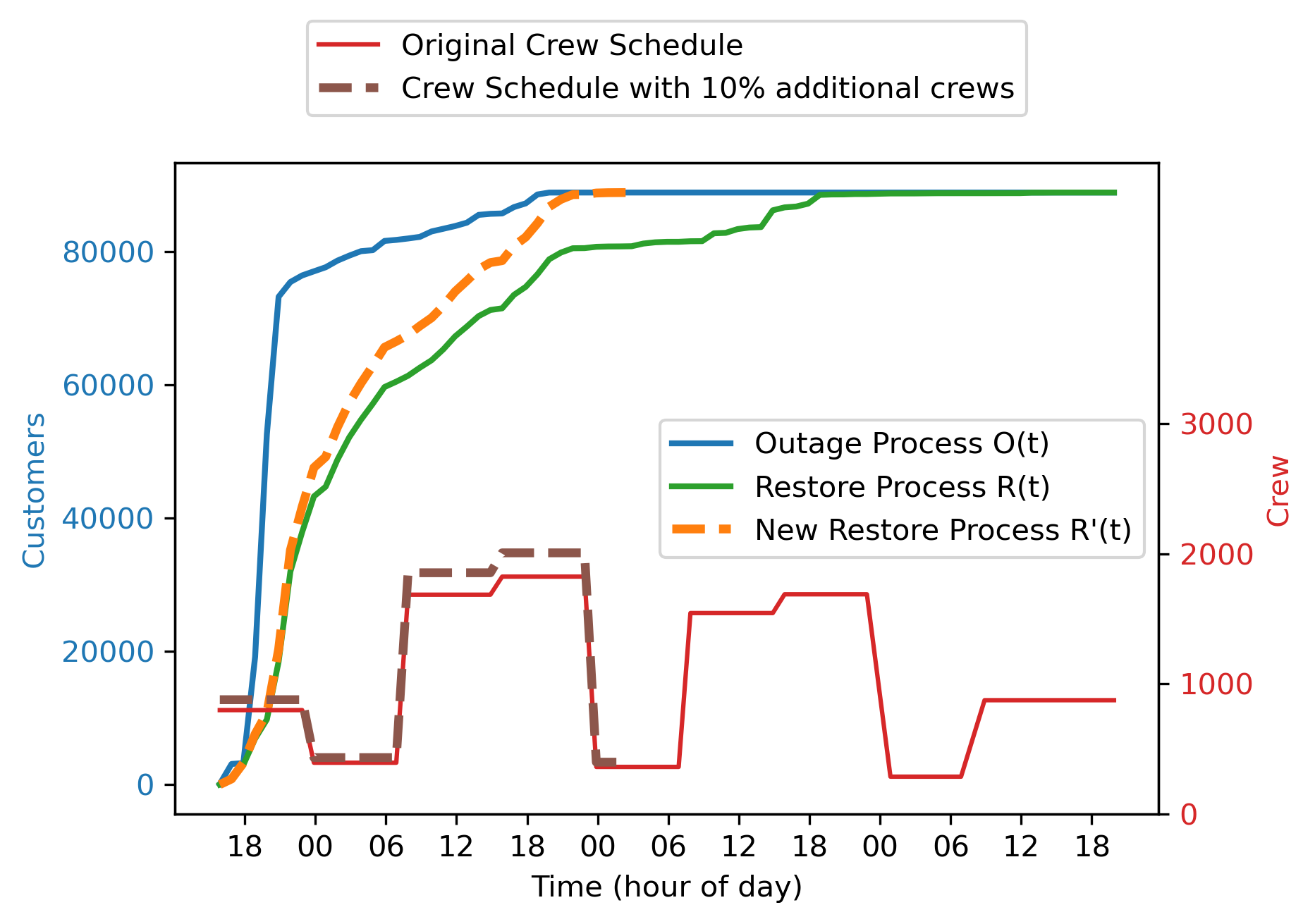
Figure 3: Reduction in REPAIR with 10% more crews

TABLE III: Rerunning storm 10 resiliency metrics

Metric	Base Case	Simulated Case
RE	1.948	1.699
AIR	0.928	0.723
REPAIR	2.876	2.422

These approximate estimates of the effects of more crews open the door to more elaborate estimates in future work. For example, as discussed in section IV, increasing the crews so much that repairs become saturated would decrease the crew efficiency. Different effects of starting restoration earlier (which may not be feasible until the storm ends), and starting at the same time but restoring faster can be readily calculated using the methods in [10]. The overall effects of hardening can also be calculated [10].

VI Conclusions

The REPAIR metric offers a unique perspective by combining storm performance with the resources deployed during restoration, an often-overlooked aspect given the ‘all hands on deck’ approach in these situations. Incorporating the REPAIR metric allows for a more comprehensive evaluation of the restoration process. This paper examines the impact of increased crew staffing levels on REPAIR outcomes. Future work should include a detailed analysis of the reduction in the area under the performance curve as a function of crew levels, providing further insights into optimal resource allocation.

References

- [1] G. Kandaperumal et al., Enabling Electric Distribution System Resiliency through Metrics-driven Black Start Restoration, 2021 IEEE Industry Applications Society Annual Meeting (IAS), Vancouver, BC, Canada
- [2] S. Pandey et al., Resiliency-Driven Proactive Distribution System Reconfiguration With Synchrophasor Data, in IEEE Transactions on Power Systems, vol. 35, no. 4, pp. 2748-2758, July 2020.
- [3] S. Pandey et al., Resilience planning simulation framework for storm hardening and recovery, IEEE PES General Meeting, Denver USA, 2022.
- [4] Y. Wei et al., Non-stationary random process for large-scale failure and recovery of power distribution, Appl. Maths.,vol.7(3), 2016, pp.233-249.
- [5] N.K. Carrington I. Dobson, Z. Wang, Extracting resilience metrics from distribution utility data using outage and restore process statistics, IEEE Trans. Power Systems, vol. 36, no. 2, Nov. 2021, pp. 5814-5823.
- [6] G. Kandaperumal, S. Pandey, A. Srivastava, AWR: Anticipate, withstand, and recover resilience metric for operational and planning decision support in electric distribution system, IEEE Trans. Smart Grid, vol. 13, no. 1, January 2022, pp. 179-190.
- [7] S. Ericson et al., Exceedance probabilities and recurrence intervals for extended power outages in the United States, National Renewable Energy Laboratory, Golden CO USA; NREL/TP-5R00-83092, 2022.
- [8] M. Abdelmalak et al., A power outage data informed resilience assessment framework, IEEE Access, vol. 11, 2023, pp. 7682-7697.
- [9] A. Ahmad, I. Dobson, Quantifying distribution system resilience from utility data: large event risk and benefits of investments, CIRED workshop, Chicago, USA Nov. 2024. Preprint arXiv:2407.10773v2 [eess.SY].
- [10] A. Ahmad, I. Dobson, Towards using utility data to quantify how investments would have increased the wind resilience of distribution systems, IEEE Trans. Power Sys., vol. 39, no. 4, 2024, pp. 5956-5968.
- [11] I. Dobson, Models, metrics, and their formulas for typical electric power system resilience events, IEEE Trans. Power Systems, vol. 38, no. 6, November 2023, pp. 5949-5952.