Distributed Generalized Nash Equilibria Learning for Online Stochastic Aggregative Games

Abstract

This paper investigates online stochastic aggregative games subject to local set constraints and time-varying coupled inequality constraints, where each player possesses a time-varying expectation-valued cost function relying on not only its own decision variable but also an aggregation of all the players’ variables. Each player can only access its local individual cost function and constraints, necessitating partial information exchanges with neighboring players through time-varying unbalanced networks. Additionally, local cost functions and constraint functions are not prior knowledge and only revealed gradually. To learn generalized Nash equilibria of such games, a novel distributed online stochastic algorithm is devised based on push-sum and primal-dual strategies. Through rigorous analysis, high probability bounds on the regret and constraint violation are provided by appropriately selecting decreasing stepsizes. Moreover, for a time-invariant stochastic strongly monotone game, it is shown that the generated sequence by the designed algorithm converges to its variational generalized Nash equilibrium (GNE) almost surely, and the time-averaged sequence converges sublinearly with high probability. Finally, the derived theoretical results are illustrated by numerical simulations.

I Introduction

Game theory has recently gained much attention in a breadth of fields, such as power grids [1], social networks [2], commodity distribution [3], and so on. In such problems, selfish players delve into optimize their individual private, yet interdependent objective functions. As important solution concepts for noncooperative games, Nash equilibrium (NE) and generalized Nash equilibrium (GNE) mathematically characterize stable and satisfactory states, from which no player possesses an incentive for unilateral deviation.

In last decades, a large body of distributed NEs and GNEs seeking algorithms in noncooperative games have sprung up [2, 4, 5, 6, 7, 8, 9, 10, 11]. In contrast to the full-decision information scenario [2, 4], where a coordinator is required to compute and broadcast the data to players, each player in the partial-decision information scenario is capable to make decisions relying only on partial estimates on decisions of others through local information exchanges between neighbouring players [5, 6, 7, 8, 9, 10, 11]. As a consequence, distributed algorithms enjoy overwhelming advantages including lower communication burden, better robustness, and privacy preservation. Note that all investigations mentioned above focused on offline games, where cost and constraint functions of rational players are assumed to be time-invariant.

However, dynamic environments are commonly encountered in various real applications, including real-time traffic networks, radio resources allocation, and online auction. In such scenarios, the cost functions and/or constraints of players often vary over time because of external factors. Consequently, online games become a hot research topic, which have been extensively investigated [12, 13, 14, 15, 16, 17]. In online games, cost and constraint functions are not known as prior knowledge, which instead are revealed to players only after the decisions of players are made at current time. Each player aims to choose its decision by repeatedly adapting other players’ decisions in a dynamic way such that its static/dynamic regret, i.e., the difference between accumulated payoff incurred by a player’s real decision and the best fixed/dynamic decision in hindsight, is minimized. Generally speaking, an online algorithm performs well if it satisfies the no-regret property, i.e., the regret is sublinear versus the learning time. To this end, a distributed primal-dual algorithm was designed in [12] to deal with online game with time-invariant constraints. Subsequently, authors in [13] proposed an online distributed learning algorithm with bandit feedback based on the mirror descent and primal-dual strategy to handle time-varying coupled inequality constraints. Moreover, as an important class of online noncooperative games, online aggregative games have attracted tremendous research interest [16, 14, 17]. Here, players’ cost functions depend both on their individual decisions and the aggregate behavior of all players. For instance, in order to defend attacks of intruders, a target is surrounded by a collection of robots, and in this case, local cost functions of robots rely on their own positions and the center of all robots’ positions. Along this line, a distributed online NE tracking algorithm with privacy preservation was devised in [17] by combining projected pseudogradient and dynamic average consensus methods. Taking local decision sets and global coupled inequality constraints into account, authors in [16] considered online aggregative games in the feedback delay case, and [14] addressed time-varying unbalanced networks.

It is noteworthy that all the aforementioned research considered online games with deterministic cost functions. However, due to various information uncertainties in practical situations, the local cost functions are often characterized as the expectation of stochastic functions. For example, in electricity markets, companies producing energy do not know the demand in advance [18]. Although there have been several works concentrated on noncooperative games with expectation-valued cost functions [19, 3, 20, 21, 22, 23], unfortunately, these algorithms are not applicable to online cases, and theoretical guarantees were usually provided only in expectation. While guarantees hold in expectation can ensure the average performance of an algorithm over substantial amounts of independent runs, they cannot preclude an extremely bad case [24, 25, 26, 27]. Additionally, towards real applications, we can perform the algorithm only in a few runs or even a single run owing to limitation on computing time or resources. For instance, in the distributed tracking problem, sensors require to accurately determine the target’s position as quickly as possible, making it desirable to run the algorithm in finite rounds [28]. These observations highlight the importance of high probability guarantees of an algorithm in a single run both theoretically and practically. However, there is little research in this direction for online stochastic games. As far as we know, a relevant work is [29], where an online distributed stochastic mirror descent algorithm was proposed to handle online stochastic noncooperative games with set constraints. It was shown that the regrets increase sublinearly with a high probability. As a result, it is crucial to establish high probability bounds on regrets to guarantee the performance of stochastic online NEs (GNEs) seeking algorithms, thus motivating our current research.

Driven by the above observations, we are going to focus on online stochastic aggregative games over time-varying unbalanced networks. Here, players aim to selfishly minimize their individual time-varying expectation-valued cost functions, while satisfying local feasible set constraints and time-varying coupled inequality constraints. Assume that players can make decisions by using their sample estimates on gradients instead of accurate gradients of cost functions. To solve this problem, a distributed online stochastic algorithm is devised based on primal-dual and push-sum schemes, which can achieve sublinear high probability bounds on regrets and constraint violation under mild conditions. When analyzing the high probability guarantees of the devised algorithm, the estimated error between the sampled gradients and exact gradients is inevitable. Note that the expectation on this related term becomes zero if the noisy gradient estimate is unbiased, thereby not influencing the regret and constraint violation bounds in expectation. Unfortunately, to establish effective high probability bounds, this error cannot be eliminated at all, which makes our analysis more technically challenging. Moreover, since the aggregative variable is unavailable to each player, additional auxiliary variables are required to track it. However, the unbalanced communication networks further complicate our ability to track the aggregative variable precisely. Meanwhile, it is also hard for players to estimate the global optimal dual variable to achieve consensus. The introduced consensus errors will affect the upper bounds of regrets and constraint violation, which must be carefully addressed. The main contributions are summarized as below.

• To our best knowledge, online stochastic aggregative games with local set constraints and time-varying shared coupled nonlinear inequality constraints are studied for the first time, where each player possesses a private time-varying expectation-valued cost function involved in an aggregative variable. In contrast to deterministic counterparts [14, 16, 17] and offline stochastic games [19, 3, 20, 21, 22, 23], the formulated problem enjoys new characteristics and broadens the scope of practical applications.

• An online distributed stochastic primal-dual push-sum algorithm is proposed. Unlike the doubly stochastic communication graphs employed in [13, 21, 29, 16, 17] to model players’ information exchanges, we study more general time-varying unbalanced graphs. For this, a push-sum idea [30] is leveraged for devising our algorithm in order to eliminate the impact on graphs’ imbalance. Moreover, our work extends [29] by considering an aggregative variable in cost functions and general time-varying convex coupled constraints.

• Under mild conditions, it is rigorously proved that the regrets and constraint violation of the proposed algorithm increase sublinearly with high probability. Additionally, the time-invariant stochastic aggregative game is considered as a special case. We show that the decision sequence generated by the algorithm converges almost surely to the variational GNE (VGNE) under strong monotonicity. Furthermore, the sublinear convergence rate in high probability of the averaged decision sequence is firstly derived. Distinctive from convergence guarantees that hold only in expectation [19, 13, 21], our high probability results benefit for ensuring the effectiveness by running the proposed algorithm in a single round, which is more mathematically and practically rigorous and desirable. Simultaneously, the theoretical analysis also becomes more complex and challenging.

The rest of this paper is organized as follows. Section II presents some preliminaries and formulates the concerned problem. Section III develops the algorithm and provides the main results. In Section IV, a numerical simulation is given to support the obtained results. Section V concludes this paper.

Notations: Denote by $\mathbb{R}^{n}$, $\mathbb{R}^{n}_{+}$, and $\mathbb{R}^{m\times n}$ the sets of $n$-dimensional real vectors, $n$-dimensional real vectors with nonnegative entries, and $m\times n$ real matrices, respectively. $\|\cdot\|$ and $\|\cdot\|_{1}$ represent standard Euclidean norm and $l_{1}$-norm, respectively. For vectors $x,y\in\mathbb{R}^{n}$, $x^{\textit{T}}$ and $\langle x,y\rangle$ denote the transpose of $x$ and standard inner product of $x,y$. Let ${\bf 1}$ and ${\bf 0}$ be compatible vectors of all entries equal to $1$ and $0$, respectively. $[N]:=\{1,\ldots,n\}$ represents the index set for an integer $N>0$. $\operatorname*{col}\{x_{1},\ldots,x_{N}\}:=(x_{1}^{\textit{T}},\ldots,x_{N}^{\textit{T}})^{\textit{T}}$. Given two functions $h_{1}$ and $h_{2}$, $h_{1}=\mathcal{O}(h_{2})$ means that there exists a constant $C>0$ such that $|h_{1}(x)|\leq C|h_{2}(x)|$ for all $x$ in their domains, and $h_{1}=o(T)$ indicates that $\lim_{T\to\infty}\frac{h_{1}}{T}=0$. For function $f(x,y):\mathbb{R}^{d}\times\mathbb{R}^{n}\to\mathbb{R}$, let $\nabla_{1}f(x,y):=\frac{\partial f(x,y)}{\partial x}$ and $\nabla_{2}f(x,y):=\frac{\partial f(x,y)}{\partial y}$ denote its gradients with respect to the first variable $x$ and the second variable $y$, respectively. Given a closed convex set $X\subset\mathbb{R}^{n}$, $\mathbf{N}_{X}(x)=\{s:s^{\textit{T}}(y-x)\leq 0,\ \forall y\in X$} denotes the normal cone of $x\in X$. Let $\Pi_{X}[x]={\arg\min}_{y\in X}\|y-x\|$ be the projection of a vector $x\in\mathbb{R}^{n}$ onto X, and $[x]_{+}:=\Pi_{\mathbb{R}^{n}_{+}}[x]$. It is well known that

$$\|\Pi_{X}[x]-\Pi_{X}[y]\|\leq\|x-y\|,\ \forall x,y\in X,$$ (1)

$$\langle x-\Pi_{X}[x],y-\Pi_{X}[x]\rangle\leq 0,\ \forall y\in X.$$ (2)

II PRELIMINARIES

II-A Graph Theory

At time instant $t$, denote by $\mathcal{G}_{t}=(\mathcal{V},\mathcal{E}_{t})$ a time-varying directed graph, where $\mathcal{V}=[N]$ is the node set and $\mathcal{E}_{t}\subset\mathcal{V}\times\mathcal{V}$ is the edge set. An edge $(j,i)\in\mathcal{E}_{t}$ if node $i$ could receive information from node $j$. The weighted adjacency matrix is $\mathcal{W}_{t}=[w_{ij,t}]\in\mathbb{R}^{N\times N}$, where $w_{ij,t}>0$ if $(j,i)\in\mathcal{E}_{t}$ and $w_{ij,t}=0$, otherwise. It is assumed $w_{ii,t}>0$ for any $i\in[N]$. A direct path from $v_{1}$ to $v_{p}$ in $\mathcal{G}_{t}$ is a sequence of distinct nodes $v_{i}$, $i\in[p]$ such that $(v_{m},v_{m+1})\in\mathcal{E}_{t}$ for all $m\in[p-1]$. $\mathcal{G}_{t}$ is called strongly connected if there exists a directed path from any node to any other node in the graph.

We make the following assumptions on the interaction networks.

Assumption 1.

             

• For any $i,j\in[N]$, there exists a constant $w\in(0,1)$ such that $w_{ij,t}\geq w$ if $w_{ij,t}>0$.

• The adjacency matrix $\mathcal{W}_{t}$ is column-stochastic, i.e., $\sum_{i=1}^{N}w_{ij,t}=1$ for all $j\in[N]$.

• There exists a constant $U>0$, such that the graph $\left(\mathcal{V},\cup_{l=0,\ldots,U-1}\mathcal{E}_{t+l}\right)$ is strongly connected.

It is worth noting that compared to previous works [13, 21, 29, 16, 17], which assumed the communication graphs to be doubly stochastic, Assumption 1 is less conservative.

II-B Problem Formulation

This section formulates online stochastic aggregative game $\Gamma_{t}:=\Gamma(\mathcal{V},X_{t},f_{t})$. Let $\mathcal{V}:=[N]$ denote the set of players. Denote by $x_{i}$ the decision of player $i$, $x:=\operatorname*{col}\{x_{i}\}_{i\in[N]}$ the joint decision of all players, and $x_{-i}:=\operatorname*{col}\{x_{i}\}_{i\in[N]\setminus i}$ the joint decision of all the players except $i$. $X_{t}:=(X_{1}\times\cdots\times X_{N})\bigcap X_{0,t}$ is the time-varying constraints of players, with $X_{i}\subset\mathbb{R}^{d_{i}}$ being the private decision set constraint of player $i$ and $X_{0,t}:=\{x=\operatorname*{col}\{x_{i}\}_{i\in[N]}\in\mathbb{R}^{d}\mid g_{t}(x):=\sum_{i=1}^{N}g_{i,t}(x_{i})\leq{\bf 0}_{m}\}$ being time-varying coupled inequality constraints. Here, $d:=\sum_{i=1}^{N}d_{i}$ and $g_{i,t}:\mathbb{R}^{d_{i}}\to\mathbb{R}^{m}$ is the private constraint function of player $i$. Then player $i$’s decision set is denoted by $X_{i,t}(x_{-i}):=\{x_{i}\in\mathbb{R}^{d}_{i}\mid(x_{i},x_{-i})\in X_{t}\}$. $f_{t}=(f_{1,t},\ldots,f_{N,t})$ represents a sequence of cost functions with $f_{i,t}:\mathbb{R}^{d_{i}}\times\mathbb{R}^{n}\to\mathbb{R}$ being the private time-varying cost function of player $i$. Specifically, $f_{i,t}(x_{i},\sigma(x)):=\mathrm{E}[F_{i,t}(x_{i},\sigma(x),\xi_{i,t}(\omega))]$, where $\sigma(x):=\frac{1}{N}\sum_{i=1}^{N}\psi_{i}(x_{i})$ is the aggregation of all players’ decision variables, in which each private function $\psi_{i}:\mathbb{R}^{d_{i}}\to\mathbb{R}^{n}$ for player $i$ is the $i$-th contribution to $\sigma(x)$, $\xi_{i,t}:\Omega_{i}\to\mathbb{R}^{q_{i}}$ is a stochastic vector defined on the probability space $(\Omega_{i},\mathscr{F}_{i},\mathrm{P}_{i})$, $F_{i,t}:\mathbb{R}^{d_{i}}\times\mathbb{R}^{n}\times\mathbb{R}^{q_{i}}\to\mathbb{R}$ is a scalar-valued function, and $\mathrm{E}$ is the expectation with respect to the probability measure $\mathrm{P}_{i}$. Denote $\sigma(x_{-i}):=\sum_{j\neq i,j=1}^{N}\psi_{j}(x_{j})$ the aggregate of all players except player $i$.

At each time $t$, all players act simultaneously to selfishly minimize its own cost function $f_{i,t}(x_{i},\sigma(x))$ within its decision set $X_{i,t}$. Hopefully, all players’ decisions reach a GNE $x_{t}^{*}=(x_{i,t}^{*},x_{-i,t}^{*})$, from which one cannot benefit from changing its decision unilaterally. Here, a GNE $x_{t}^{*}$ of $\Gamma_{t}:=\Gamma(\mathcal{V},X_{t},f_{t})$ satisfies that for any $i\in[N]$, it holds

$$f_{i,t}(x_{i,t}^{*},\sigma(x_{t}^{*}))\leq f_{i,t}(x_{i},\psi_{i}(x_{i})+\sigma(x_{-i,t}^{*})),$$

$$\forall x_{i}\in X_{i,t}(x_{-i,t}^{*}).$$

Next, some standard assumptions on the studied game are listed, which are also made in [13, 16, 12, 14, 17].

Assumption 2.

          

• The sets $X_{i}$, $i\in[N]$, are nonempty, convex, and compact.

• The feasible set $X_{t}$ is nonempty and satisfies Slater’s constraint qualification.

• For any $i\in[N]$ and $t\geq 0$, $f_{i,t}(x_{i},\sigma)$ is differentiable in $(x_{i},\sigma)\in X_{i}\times\mathbb{R}^{n}$. Moreover, $f_{i,t}(x_{i},\sigma(x))$ is convex in $x_{i}\in X_{i}$ for any given $x_{-i}\in\mathbb{R}^{d-d_{i}}$.

• For any $i\in[N]$ and $t\geq 0$, $g_{ij,t}(x_{i})$ is differentiable and convex on $X_{i}$, where $g_{ij,t}$ is the $j$-th component of $g_{i,t}$. Moreover, $\nabla g_{i,t}$ is uniformly bounded, i.e., there exists $M>0$ such that for any $x_{i}\in X_{i}$, $\|\nabla g_{i,t}(x_{i})\|\leq M$, where $\nabla g_{i,t}(x_{i}):=(\nabla g_{i1,t}(x_{i}),\ldots,\nabla g_{im,t}(x_{i}))$.

• For any $i\in[N]$, $\psi_{i}$ is differentiable and $L_{\sigma}$-Lipschitz continuous $(L_{\sigma}>0)$, i.e.,

  $$\|\psi_{i}(x)-\psi_{i}(x^{\prime})\|\leq L_{\sigma}\|x-x^{\prime}\|,\ \forall x,x^{\prime}\in X_{i}.$$

It can be further obtained from Assumption 2 that for any $i\in[N]$ and $x_{i}\in X_{i}$, there exists $L>0$ such that

$$\|x_{i}\|\leq L,\ \|g_{i,t}(x_{i})\|\leq L.$$ (3)

In fact, $x_{t}^{*}=(x_{i,t}^{*},x_{-i,t}^{*})$ is a GNE if and only if $x_{i,t}^{*}$ is an resolution of the following optimization problem

$$\min_{x_{i}\in X_{i}}~f_{i,t}(x_{i},\psi_{i}(x_{i})+\sigma(x_{-i,t}^{*}))$$

$$\text{s.t.}~g_{i,t}(x_{i})+\sum_{j\neq i,j=1}^{N}g_{j,t}(x_{j,t}^{*})\leq{\bf 0}.$$ (4)

Define the Lagrangian function of problem (II-B) for player $i$ as

$$L_{i,t}(x_{i},\mu_{i,t};x_{-i,t}^{*}) :=f_{i,t}(x_{i},\psi_{i}(x_{i})+\sigma(x_{-i,t}^{*}))$$

$$\quad+{\mu_{i,t}}^{\textit{T}}\left(g_{i,t}(x_{i})+\sum_{j\neq i,j=1}^{N}g_{j,t}(x_{j,t}^{*})\right),$$

where $\mu\in\mathbb{R}^{m}_{+}$ is the Lagrange multiplier (dual variable) associated with the coupled constraints. Then if $x_{t}^{*}=(x_{i,t}^{*},x_{-i,t}^{*})$ is a GNE of $\Gamma_{t}$, by Karush-Kuhn-Tucker (KKT) conditions, there exit multipliers $\mu_{i,t}^{*}$, $i\in[N]$ satisfying

$${\bf 0}\in\nabla_{x_{i}}f_{i,t}(x_{i,t}^{*},\sigma(x_{t}^{*}))+\nabla g_{i}(x_{i,t}^{*})\mu_{i,t}^{*}+\mathbf{N}_{X_{i}}(x_{i,t}^{*}),$$

$${\bf 0}\in-g_{t}(x_{t}^{*})+\mathbf{N}_{\mathbb{R}^{m}_{+}}(\mu_{i,t}^{*}),\ i\in[N],$$ (5)

where $\nabla_{x_{i}}f_{i,t}(x_{i,t}^{*},\sigma(x_{t}^{*})):=\nabla_{1}f_{i,t}(x_{i,t}^{*},\sigma(x_{t}^{*}))+\frac{\nabla\psi_{i}(x_{i,t}^{*})}{N}\nabla_{2}f_{i,t}(x_{i,t}^{*},\sigma(x_{t}^{*}))$. In the KKT conditions (II-B), each $\mu_{i,t}^{*}$, $i\in[N]$ conforms to the same $g_{t}(x_{t}^{*})$, indicating that the system is ill-posed. Instead, a VGNE satisfying (II-B) for some $\mu_{t}^{*}:=\mu_{i,t}^{*}=\mu_{j,t}^{*}$ is economically justifiable [31]. As a consequence, it has been commonly practical to seek the VGNE rather than the GNE [12, 13, 14, 16]. From the perspective of variational inequality, it follows from Assumption 2 that $x_{t}^{*}$ is a VGNE of $\Gamma_{t}$ if and only if $x_{t}^{*}$ is a solution to the variational inequality

$$G_{t}(x_{t}^{*})^{\textit{T}}(x-x_{t}^{*})\geq 0,\ \forall x\in X_{t},$$ (6)

where $G_{t}(x):=\operatorname*{col}\{\nabla_{x_{i}}f_{i,t}(x_{i},\sigma(x))\}_{i\in[N]}$ is the pseudo-gradient mapping of $\Gamma_{t}$. Furthermore, the existence of $x_{t}^{*}$ can be guaranteed by Assumption 2 [32].

However, in online game $\Gamma_{t}$, for each $i\in[N]$, $f_{i,t}$ and $g_{i,t}$ are revealed to player $i$ only after making its decision $x_{i,t}$ at time $t$. It is impossible for players to pre-compute a GNE $(x_{i,t}^{*},x_{-i,t}^{*})$ of $\Gamma_{t}:=\Gamma(\mathcal{V},X_{t},f_{t})$. Therefore, a new performance metric, called regret, is commonly employed for online game. Motivated by [13], define the static regret for player $i$ as

$$\mathcal{R}_{i}(T):=\sum_{t=1}^{T}[f_{i,t}(x_{i,t},\sigma(x_{t})))-f_{i,t}(x_{i}^{\star},\psi_{i}(x_{i}^{\star})+\sigma(x_{-i,t})],$$ (7)

where $T$ is the learning time horizon and $x^{\star}_{i}$ is the optimal static decision in hindsight solving

$$\min_{x_{i}\in X_{i}}~\sum_{t=1}^{T}f_{i,t}(x_{i},\psi_{i}(x_{i})+\sigma(x_{-i,t}))$$

$$\text{s.t.}~g_{i,t}(x_{i})+\sum_{j\neq i,j=1}^{N}g_{j,t}(x_{j,t})\leq{\bf 0}_{m},\ \forall t\in[T].$$ (8)

In order to ensure that problem (II-B) is feasible, the set $\bigcap_{t=1}^{T}X_{i,t}(x_{-i,t})$ is assumed to be nonempty.

Furthermore, since the decisions of players need to satisfy coupled inequality constraints, it is indispensable to introduce a kind of regret involves this constraints. Specifically, the following constraint violation metric is given

$$\mathcal{R}_{g}(T):=\left\|\left[\sum_{t=1}^{T}g_{t}(x_{t})\right]_{+}\right\|.$$ (9)

Intuitively, the regret (7) of player $i$ reflects the difference between player $i$’s actual cumulative payoff and optimal cumulative payoff. Moreover, definition (9) implicitly allows constraint violations at certain times to be compensated by strictly feasible decisions at other times. In general, an online algorithm is considered to be no-regret if all regrets of players and constraint violation are sublinear with respect to $T$, i.e., $\mathcal{R}_{i}(T)=o(T)$ and $\mathcal{R}_{g}(T)=o(T)$. The goal of this paper is to design an online algorithm ensuring that $\mathcal{R}_{i}(T)$ and $\mathcal{R}_{g}(T)$ increase sublinearly with high probability.

To proceed, define

$$p_{i,t}(x_{i},y):=\bigg{(}\nabla_{1}f_{i,t}(x_{i},\sigma)+\frac{\nabla\psi_{i}(x_{i})}{N}\nabla_{2}f_{i,t}(x_{i},\sigma)\bigg{)}\bigg{|}_{\sigma=y}.$$

One can see that

$$\nabla_{x_{i}}f_{i,t}(x_{i},\sigma(x))=p_{i,t}(x_{i},\sigma(x)).$$

Assumption 3.

For any $i\in[N]$ and $t\geq 0$, $p_{i,t}(x_{i},y)$ is $L_{f}$-Lipschitz continuous $(L_{f}>0)$ with respect to $y$ for any given $x_{i}\in X_{i}$, i.e.,

$$\|p_{i,t}(x_{i},y)-p_{i,t}(x_{i},y^{\prime})\|\leq L_{f}\|y-y^{\prime}\|,\ \forall y,y^{\prime}\in\mathbb{R}^{n}.$$

Assumption 3 is commonly employed in existing studies [16, 14, 17, 21].

II-C High Probability Bound

Definition 1.

[29](High probability bounds) For regrets $\mathcal{R}_{i}(T),i\in[N]$ and constraint violation $\mathcal{R}_{g}(T)$, $\mathcal{R}_{i}(T)$ and $\mathcal{R}_{g}(T)$ are called to have high probability bounds if for any $\delta\in(0,1)$, there hold that $\mathcal{R}_{i}(T)\leq\mathcal{O}\left(r(T)\left(\ln\frac{1}{\delta}\right)^{s}\right)$ and $\mathcal{R}_{g}(T)\leq\mathcal{O}\left(r(T)\left(\ln\frac{1}{\delta}\right)^{s}\right)$ with probability at least $1-\delta$ for some function $r:\mathbb{R}\rightarrow\mathbb{R}$ and $s\in[0,1]$. Moreover, if $r(T)$ is sublinear with respect to $T$, i.e., $r(T)=o(T)$, $\mathcal{R}_{i}(T)$ and $\mathcal{R}_{g}(T)$ are called to increase sublinearly with high probability.

In the stochastic scenario, due to the lack of closed-form expressions for gradients of expectation-valued cost functions, each player $i$ can only access the noisy gradient of its cost function $f_{i,t}(x_{i},y)$, denoted by $q_{i}^{t}(x_{i},y,\xi_{i,t})$. To facilitate this, we require $F_{i}(x_{i},\sigma,\xi_{i,t})$ to be differentiable in $(x_{i},\sigma)\in X_{i}\times\mathbb{R}^{n}$ for any given $\xi_{i,t}\in\mathbb{R}^{q_{i}}$. For function $F_{i,t}(x_{i},\sigma,\xi_{i,t})$, let $\nabla_{1}F_{i,t}(x_{i},\sigma,\xi_{i,t}):=\frac{\partial F_{i,t}(x_{i},\sigma,\xi_{i,t})}{\partial x_{i}}$ and $\nabla_{2}F_{i,t}(x_{i},\sigma,\xi_{i,t}):=\frac{\partial F_{i,t}(x_{i},\sigma,\xi_{i,t})}{\partial\sigma}$ denote gradients with respect to the first variable $x_{i}$ and the second variable $\sigma$, respectively. Then specifically,

$$q_{i}^{t}(x_{i},y,\xi_{i,t}) :=\bigg{(}\nabla_{1}F_{i,t}(x_{i},\sigma,\xi_{i,t})$$

$$\quad+\frac{\nabla\psi_{i}(x_{i})}{N}\nabla_{2}F_{i,t}(x_{i},\sigma,\xi_{i,t})\bigg{)}\bigg{|}_{\sigma=y}.$$

Define the natural filtration

$$\mathscr{F}_{0}:=\{\emptyset,\Omega\},$$

$$\mathscr{F}_{t}:=\sigma\{\xi_{i,s}:\forall i\in[N],0\leq s\leq t-1\},\ \forall t\geq 1.$$ (10)

Assumption 4.

For any $t\geq 0$, $i\in[N]$, $x_{i}\in X_{i}$, $y_{i}\in\mathbb{R}^{q_{i}}$, and $x_{i},y\in\mathscr{F}_{t}$,

• $\mathrm{E}[q_{i,t}(x_{i},y,\xi_{i,t})|\mathscr{F}_{t}]=p_{i,t}(x_{i},y)$.

• $\mathrm{E}[\exp(\|q_{i,t}(x_{i},y,\xi_{i,t})-p_{i,t}(x_{i},y)\|^{2}/\iota^{2})|\mathscr{F}_{t}]\leq\exp(1)$ for some constant $\iota>0$.

• $\|q_{i,t}(x_{i},y,\xi_{i,t})\|\leq S$ for some $S>0$.

By Jensen’s inequality, it follows from Assumption 4-i) and 4-iii) that $\|p_{i,t}(x_{i},\sigma(x)\|\leq S$. Assumption 4-i) indicates that the noisy gradient $q_{i}^{t}(x_{i},y,\xi_{i,t})$ is conditionally unbiased with respect to $\mathscr{F}_{t}$. Assumption 4-ii) characterizes a sub-Gaussian noise model, where the tail behavior of the noise distribution is dominated by tails of a Gaussian distribution. Moreover, using the Jensen’s inequality, Assumption 4-ii) implies that $\mathrm{E}[\|q_{i,t}(x_{i},y,\xi_{i,t})-p_{i,t}(x_{i},y)\|^{2}]\leq\iota^{2}$, which is utilized to analyze the convergence of distributed stochastic algorithms in expectation [19, 3, 20, 21, 22, 23]. However, Assumption 4-ii) is frequently made in literature to establish finer high probability guarantees, which is highly relevant in practice [25, 27, 26, 29]. In fact, the noises that follow the uniform distribution over a compact set or Gaussian distribution satisfy the sub-Gaussian noise model. Also, in real-world applications, various estimation methods exist to achieve stochastic gradients that satisfy Assumption 4, such as the score function estimators and pathwise derivative estimator [33]. Assumption 4-iii) requires the uniform boundedness of noises, which is reasonable, particularly in scenarios such as measurement noises in sensor networks and fluctuations of market demands in economic problems. It is noteworthy that Assumption 4-iii) was also employed in prior works [34, 23] to derive high probability convergence results.

III MAIN RESULTS

This section provides proposes an online distributed stochastic algorithm for our studied games, following by the high probabilities bounds on its regrets and constraint violation.

To begin with, for each player $i\in[N]$, the regularized Lagrangian function at time instant $t$ is defined as

$$\mathcal{L}_{i,t}(x_{i},\mu;x_{-i}):=f_{i,t}(x_{i},\sigma(x))+\mu^{\textit{T}}g_{t}(x)-\frac{\beta}{2}\|\mu\|^{2},$$ (11)

where $\mu\in\mathbb{R}^{m}_{+}$ is the Lagrange multiplier (dual variable) associated with the coupled constraints and $\beta>0$ is the regularization parameter. A standard primal-dual algorithm to seek a saddle point of $\mathcal{L}_{i,t}$ can be designed as

$$x_{i,t+1} =\Pi_{X_{i}}[x_{i,t}-\alpha_{t}(p_{i,t}(x_{i,t},\sigma(x_{t}))+\nabla g_{i}(x_{i,t})\mu_{t})],$$ (12a)

$$\mu_{t+1} =[\mu_{t}+\gamma_{t}(g_{t}(x_{t})-\beta_{t}\mu_{t})]_{+},$$ (12b)

where $\alpha_{t}>0$ and $\gamma_{t}>0$ are stepsizes utilized in the primal and dual updates, respectively. However, in algorithm (12), it is noted that the exact gradient $p_{i,t}(x_{i,t},\sigma(x_{t}))$ is usually unavailable. Moreover, each individual player cannot access the information on global aggregative variable $\sigma(x_{t})$, nonlinear constraint function $g_{t}(x_{t})$, and common Lagrange multiplier $\mu_{t}$, thus requiring a central unit to compute and communicate with all the players. To this end, i) the stochastic sample gradient $q_{i,t}$ rather than the exact gradient $p_{i,t}$ is utilized. ii) A local copy $\mu_{i,t}\in\mathbb{R}^{m}$ of the multiplier $\mu_{t}$ is introduced, and the dynamic consensus technique is incorporated to enforce consensus among $\mu_{i,t}$’s. iii) By virtue of the push-sum protocol [30], the auxiliary variable $z_{i,t}\in\mathbb{R}$ is introduced, which aims to eliminate the imbalance of the communication graphs through tracking the right-hand eigenvector of $\mathcal{W}_{t}$ related to the eigenvalue ${\bf 1}$. iv) Motivated by the idea of gradient tracking [35], the variable $\sigma_{i,t}\in\mathbb{R}^{n}$ of player $i$ is employed to track $\sigma(x_{t})$. To conclude, the developed online distributed stochastic primal-dual push-sum algorithm is presented in Algorithm 1.

Algorithm 1 is distributed since each player is capable to update its variables based solely on local information exchanges. It is straightforward to observe that $x_{i,t}$ and $\sigma_{i,t}$ are adapted to $\mathscr{F}_{t}$, while $\mu_{i,t}$ is adapted to $\mathscr{F}_{t-1}$.

Algorithm 1 Online Distributed Stochastic Primal-dual Push-sum

Set $T\geq 4$. Each player $i$, $i\in[N]$ maintains variables $z_{i,t}\in\mathbb{R}$, $x_{i,t}\in\mathbb{R}^{d_{i}}$, $\mu_{i,t}\in\mathbb{R}^{m}$, and $\sigma_{i,t}\in\mathbb{R}^{n}$ at time $t=0,1,\ldots,T$.

Initialization: For any $i\in[N]$, initialize $z_{i,0}=1$, $x_{i,0}\in X_{i}$, $\mu_{i,0}={\bf 0}_{m}$, and $\sigma_{i,0}=\psi_{i}(x_{i,0})$.

Iteration: For $t\geq 0$, each player $i$ updates as follows:

$$z_{i,t+1} =\sum_{j=1}^{N}w_{ij,t}z_{j,t},$$ (13a)

$$\hat{\mu}_{i,t} =\sum_{j=1}^{N}w_{ij,t}\mu_{j,t},\ \hat{\sigma}_{i,t}=\sum_{j=1}^{N}w_{ij,t}\sigma_{j,t},$$ (13b)

$$s_{i,t+1} =q_{i,t}\left(x_{i,t},\frac{\hat{\sigma}_{i,t}}{z_{i,t+1}},\xi_{i,t}\right)+\nabla g_{i,t}(x_{i,t})\frac{\hat{\mu}_{i,t}}{z_{i,t+1}},$$ (13c)

$$x_{i,t+1} =\Pi_{X_{i}}[x_{i,t}-\alpha_{t}s_{i,t+1}],$$ (13d)

$$\mu_{i,t+1} =[\hat{\mu}_{i,t}+\gamma_{t}(g_{i,t}(x_{i,t})-\beta_{t}\hat{\mu}_{i,t})]_{+},$$ (13e)

$$\sigma_{i,t+1} =\hat{\sigma}_{i,t}+\psi_{i}(x_{i,t+1})-\psi_{i}(x_{i,t}),$$ (13f)

where $\alpha_{t}$, $\beta_{t}$, and $\gamma_{t}$ are non-increasing parameters to be determined.

Remark 1.

The utilization of noisy gradients, as opposed to exact gradients, can significantly affect the performance of the algorithm, potentially preventing it from converging. Meanwhile, the additional noise term also contributes to the technical challenge of our analysis. Moreover, in the dual update (13e), an additional term $-\gamma_{t}\beta_{t}\hat{\mu}_{i,t}$ appears, which originates from the regularized Lagrangian function (11). In fact, this is typically incorporated to guarantee the boundedness of dual variable $\mu_{i,t}$. Furthermore, note that the global information $\sigma(x_{t})$, and thus $\nabla_{1}F_{i,t}(x_{i,k},\sigma(x_{t}),\xi_{i,t})$ and $\nabla_{2}F_{i,t}(x_{i,k},\sigma(x_{t}),\xi_{i,t})$ are not accessible to any individual player in the distributed framework. Hence, we introduce $\sigma_{i,t}$ to track $\sigma(x_{t})$ for player $i$, which further complicates the algorithm. Additionally, under unbalanced graphs where $\mathcal{W}_{t}=[w_{ij,t}]$ is column-stochastic, $\sum_{j=1}^{N}w_{ij,t}\mu_{j,t}$, as multipliers in the Lagrangian function, will eventually reach different vector values. Hence, an identical Lagrange multiplier cannot be estimated as expected. Similarly, $\sum_{j=1}^{N}w_{ij,t}\sigma_{j,t}$ cannot successfully track $\sigma(x_{k})$. To bypass these challenges, the push-sum approach is adopted to address the imbalance of the interaction graphs. Correspondingly, it is necessary to analyze the introduced consensus errors, which will also bring additional difficulties.

Remark 2.

In [14], a distributed online push-sum mirror descent algorithm was devised for online aggregative games in deterministic case. In contrast, this work focuses on stochastic cost functions. Furthermore, unlike existing offline counterparts in [19, 21], where convergence in expectation was established, we delve into providing high probability bounds of regrets and constraint violation under the sub-Gaussian noise model to ensure the effectiveness of Algorithm 1, which enhances practicality while making theoretical analysis more complex and challenging.

In what follows, some useful lemmas are provided. Before this, define

$$r:=\inf_{t=0,1,\ldots}\left(\min_{i\in[N]}\left\{\mathcal{W}_{t}\cdots\mathcal{W}_{0}{\bf 1}_{N}\right\}_{i}\right).$$

Under Assumption 1, it follows from Lemma 4 in [30] that $r\geq\frac{1}{N^{NU}}$.

The following lemma provides upper bounds on the variables $z_{i,t}$ and $\mu_{i,t}$.

Lemma 1.

Under Assumptions 1 and 2, for any $t\geq 0$ and $i\in[N]$, there holds

$$r\leq z_{i,t}\leq N,\ r\leq 1,$$ (14)

$$\|\mu_{i,t}\|\leq\frac{z_{i,t+1}L}{\beta_{t}r^{2}w},\ \|\hat{\mu}_{i,t}\|\leq\frac{z_{i,t+1}L}{\beta_{t}r^{2}}.$$ (15)

Proof.

See Appendix A. ∎

Define

$$\tilde{\mu}_{i,t+1}:=\frac{\hat{\mu}_{i,t}}{z_{i,t+1}},\ \bar{\mu}_{t}:=\frac{1}{N}\sum_{i=1}^{N}\mu_{i,t},$$

$$\tilde{\sigma}_{i,t+1}:=\frac{\hat{\sigma}_{i,t}}{z_{i,t+1}},\ \bar{\sigma}_{t}:=\frac{1}{N}\sum_{i=1}^{N}\sigma_{i,t}.$$

We next estimate errors $\|\tilde{\mu}_{i,t+1}-\bar{\mu}_{t}\|$ and $\|\tilde{\sigma}_{i,t+1}-\bar{\sigma}_{t}\|$. (13e) and (13e) can be rewritten as

$$\mu_{i,t+1} =\hat{\mu}_{i,t}+\varepsilon_{\mu_{i,t+1}},$$ (16)

$$\sigma_{i,t+1} =\hat{\sigma}_{i,t}+\varepsilon_{\sigma_{i,t+1}},$$ (17)

where

$$\varepsilon_{\mu_{i,t+1}} :=[\hat{\mu}_{i,t}+\gamma_{t}(g_{i,t}(x_{i,t})-\beta_{t}\hat{\mu}_{i,t})]_{+}-\hat{\mu}_{i,t},$$ (18)

$$\varepsilon_{\sigma_{i,t+1}} :=\psi_{i}(x_{i,t+1})-\psi_{i}(x_{i,t}).$$ (19)

Lemma 2.

Under Assumptions 1 and 2, there holds

$$\|\tilde{\mu}_{i,t+1}-\bar{\mu}_{t}\| \leq\frac{16N\sqrt{m}L}{r}\sum_{k=1}^{t}\vartheta^{t-k}\gamma_{k-1},$$ (20)

$$\|\tilde{\sigma}_{i,t+1}-\bar{\sigma}_{t}\| \leq\frac{8}{r}\bigg{(}\vartheta^{t}\|\sigma_{0}\|_{1}+N\sqrt{n}L_{\sigma}S\sum_{k=1}^{t}\vartheta^{t-k}\alpha_{k-1}$$

$$\quad+\frac{N\sqrt{n}L_{\sigma}LM}{r^{2}}\sum_{k=1}^{t}\vartheta^{t-k}\frac{\alpha_{k-1}}{\beta_{k-1}}\bigg{)},$$ (21)

where $\vartheta\leq\left(1-\frac{1}{N^{NU}}\right)^{\frac{1}{NU}}\in(0,1)$.

Proof.

See Appendix B. ∎

Next, a crucial lemma is derived, which provides the high probability bound of the term $\Delta_{t}:=\langle p_{i,t}(x_{i,t},\tilde{\sigma}_{i,t+1})-q_{i,t}(x_{i,t},\tilde{\sigma}_{i,t+1},\xi_{i,t}),x_{i,t}-x_{i}\rangle$, by elaborately leveraging some stochastic analysis and inequality techniques.

Lemma 3.

Under Assumptions 2 and 4, for any $x_{i}\in X_{i}$ and $0<\delta<1$, with probability at least $1-\delta$,

$$\sum_{t=1}^{T}\alpha_{t}\langle p_{i,t}(x_{i,t},\tilde{\sigma}_{i,t+1})-q_{i,t}(x_{i,t},\tilde{\sigma}_{i,t+1},\xi_{i,t}),x_{i,t}-x_{i}\rangle$$

$$\leq 2L\iota\sum_{t=1}^{T}\alpha_{t}^{2}+2L\iota\ln\frac{1}{\delta}.$$ (22)

Proof.

See Appendix C. ∎

The recursive inequality relations on the errors of the primal and dual variables are revealed in the subsequent two lemmas, respectively.

Lemma 4.

Under Assumptions 1-3, 4-i), and 4-iii), for any $x_{i}\in X_{i}$, there holds

$$\langle p_{i,t}(x_{i,t},\sigma(x_{t})),x_{i,t}-x_{i}\rangle$$

$$\leq S^{2}\alpha_{t}+\frac{16Ll_{f}}{r}\|\sigma_{0}\|_{1}\vartheta^{t}$$

$$\quad+\frac{16LNSl_{f}\sqrt{n}L_{\sigma}}{r}\sum_{k=1}^{t}\vartheta^{t-k}\alpha_{k-1}$$

$$\quad+\frac{16N\sqrt{n}L_{\sigma}L^{2}l_{f}M}{r^{3}}\sum_{k=1}^{t}\vartheta^{t-k}\frac{\alpha_{k-1}}{\beta_{k-1}}$$

$$\quad+\frac{32L^{2}N\sqrt{m}}{r}\sum_{k=1}^{t}\vartheta^{t-k}\gamma_{k-1}$$

$$\quad+\langle p_{i,t}(x_{i,t},\tilde{\sigma}_{i,t+1}))-q_{i,t}(x_{i,t},\tilde{\sigma}_{i,t+1},\xi_{i,t}),x_{i,t}-x_{i}\rangle$$

$$\quad+\frac{1}{2\alpha_{t}}\|x_{i}-x_{i,t}\|^{2}-\frac{1}{2\alpha_{t}}\|x_{i}-x_{i,t+1}\|^{2}$$

$$\quad+\bar{\mu}_{t}^{\textit{T}}(g_{i,t}(x_{i})-g_{i,t}(x_{i,t}))+\frac{M^{2}L^{2}}{r^{4}}\frac{\alpha_{t}}{\beta_{t}^{2}}.$$ (23)

Proof.

See Appendix D. ∎

Lemma 5.

Under Assumptions 1 and 2, there holds

$$\|\bar{\mu}_{t+1}-\mu\|^{2}$$

$$\leq\|\bar{\mu}_{t}-\mu\|^{2}+2\left(1+\frac{2}{r}\right)\left(1+\frac{N^{2}}{r^{4}}\right)L^{2}\gamma_{t}^{2}$$

$$\quad+\frac{32N\sqrt{m}L^{2}}{r}\left(2+\frac{N}{r^{2}}\right)\gamma_{t}\sum_{k=1}^{t}\vartheta^{t-k}\gamma_{k-1}$$

$$\quad+\frac{2\gamma_{t}}{N}g_{t}(x_{t})^{\textit{T}}(\bar{\mu}_{t}-\mu)+N\gamma_{t}\beta_{t}\|\mu\|^{2}.$$ (24)

Proof.

See Appendix E. ∎

Equipped with the above preparations, we are going to provide the high probability bounds on $\mathcal{R}_{i}(T)$ and $\mathcal{R}_{g}(T)$.

Lemma 6.

Let Assumptions 1-4 be satisfied. For any $i\in[N]$ and $0<\delta<1$, with probability at least $1-\delta$, the regret (7) and constraint violation (9) generated by Algorithm 1 are bounded by

$$\mathcal{R}_{i}(T) \leq S_{1}(T)+S_{2}(T)+S_{3}(T),$$ (25)

$$\mathcal{R}_{g}(T) \leq\sqrt{S_{4}(T)(S_{1}(T)+S_{2}(T)+S_{5}(T))},$$ (26)

where

$$S_{1}(T) :=\frac{16Ll_{f}\vartheta\|\sigma_{0}\|_{1}}{r(1-\vartheta)}+A_{1}\sum_{t=1}^{T}\alpha_{t-1}+A_{2}\sum_{t=1}^{T}\gamma_{t-1}$$

$$\quad+2L\iota\frac{\sum_{t=1}^{T}\alpha_{t}^{2}}{\alpha_{T}}+\frac{2L^{2}}{\alpha_{T+1}}+\frac{M^{2}L^{2}}{r^{4}}\sum_{t=1}^{T}\frac{\alpha_{t}}{\beta_{t}^{2}}$$

$$\quad+\frac{16N\sqrt{n}L_{\sigma}L^{2}l_{f}M}{r^{3}(1-\vartheta)}\sum_{t=1}^{T}\frac{\alpha_{t-1}}{\beta_{t-1}},$$

$$S_{2}(T) :=\frac{2L\sigma\ln\frac{1}{\delta}}{\alpha_{T}},$$

$$S_{3}(T) :=\frac{NL^{2}}{2r^{4}w^{2}\gamma_{T+1}\beta_{T+1}^{2}},$$

$$S_{4}(T) :=2N^{2}\sum_{t=1}^{T}\beta_{t},$$

$$S_{5}(T) :=\frac{N^{2}L^{2}}{r^{4}w^{2}\gamma_{T+1}\beta_{T+1}^{2}}+\frac{T^{2}L^{2}}{N\gamma_{T+1}\left(\sum_{t=1}^{T}\beta_{t}\right)^{2}},$$

with $A_{1}:=S^{2}+\frac{16LNSl_{f}\sqrt{n}L_{\sigma}}{r(1-\vartheta)}$ and $A_{2}:=\left(1+\frac{2}{r}\right)\left(1+\frac{N^{2}}{r^{4}}\right)NL^{2}+\frac{16N\sqrt{m}L^{2}}{r(1-\vartheta)}\left(2(N+1)+\frac{N^{2}}{r^{2}}\right)$.

Proof.

See Appendix F. ∎

Now, it is ready to present the main results of this paper.

Theorem 1.

Suppose that Assumptions 1-4 hold. Let $\alpha_{0}=\beta_{0}=\gamma_{0}=1$, and for $t\geq 1$,

$$\alpha_{t}=\frac{1}{t^{a_{1}}},\ \beta_{t}=\frac{1}{t^{a_{2}}},\ \gamma_{t}=\frac{1}{t^{a_{3}}},$$ (27)

where $0<a_{1},a_{3}<1$, $a_{1}>2a_{2}>0$, and $2a_{2}+a_{3}<1$, then for any $i\in[N]$ and $0<\delta<1$, with probability at least $1-\delta$, the sequence $\{x_{i,1},\ldots,x_{i,T}\}$ generated by Algorithm 1 satisfies

$$\mathcal{R}_{i}(T) =\mathcal{O}\bigg{(}T^{\max\{a_{1},1-a_{3},1-a_{1}+2a_{2},2a_{2}+a_{3}\}}+T^{a_{1}}\ln\frac{1}{\delta}\bigg{)},$$ (28)

$$\mathcal{R}_{g}(T) =\mathcal{O}\bigg{(}T^{\max\{1-\frac{a_{2}+a_{3}}{2},1-\frac{a_{1}+a_{2}}{2},\frac{1+a_{1}+a_{2}}{2},\frac{1-a_{1}+a_{3}}{2}\}}$$

$$\quad+T^{\frac{a_{1}+a_{2}+a_{3}}{2}}\sqrt{\ln\frac{1}{\delta}}\bigg{)}.$$ (29)

Proof.

Note that for any $0<a\neq 1$,

$$\sum_{t=1}^{T}\frac{1}{t^{a}}\leq 1+\int_{1}^{T}\frac{1}{t^{a}}dt\leq 1+\frac{T^{1-a}-1}{1-a}\leq\frac{T^{1-a}}{1-a},$$ (30)

and for any $T\geq 4$ and $a\in(0,1/2]$,

$$\sum_{t=1}^{T}\frac{1}{t^{a}}\geq\int_{1}^{T}\frac{1}{t^{a}}dt=\frac{T^{1-a}-1}{1-a}\geq\frac{T^{1-a}}{2(1-a)}.$$ (31)

Therefore, simple manipulations lead to

$$S_{1}(T)=\mathcal{O}(T^{1-a_{3}}+T^{1-a_{1}+2a_{2}}+T^{a_{1}}),$$

$$S_{2}(T)=\mathcal{O}\left(T^{a_{1}}\ln\frac{1}{\delta}\right),\ S_{3}(T)=\mathcal{O}(T^{2a_{2}+a_{3}}),$$

$$S_{4}(T)=\mathcal{O}(T^{1-a_{2}}),\ S_{5}(T)=\mathcal{O}(T^{2a_{2}+a_{3}}).$$

Subsequently, by virtue of Lemma 6, assertions (28) and (29) can be derived. This completes the proof. ∎

By specifying parameters $a_{1}$, $a_{2}$, and $a_{3}$ in Theorem 1, the regret $\mathcal{R}_{i}(T)$ can reach a good upper bound.

Corollary 1.

Under the same conditions as in Theorem 1, let $a_{1}=\frac{1}{2}+a_{2}$, $a_{3}=\frac{1}{2}-a_{2}$, and $a_{2}\in(0,\frac{1}{2})$, then for any $i\in[N]$ and $0<\delta<1$, with probability at least $1-\delta$, there holds

$$\mathcal{R}_{i}(T) =\mathcal{O}\left(T^{\frac{1}{2}+a_{2}}+T^{\frac{1}{2}+a_{2}}\ln\frac{1}{\delta}\right),$$ (32)

$$\mathcal{R}_{g}(T) =\mathcal{O}\bigg{(}T^{\frac{3}{4}+a_{2}}+T^{\frac{1+a_{2}}{2}}\sqrt{\ln\frac{1}{\delta}}\bigg{)},$$ (33)

Proof.

Let $a_{1}=\frac{1}{2}+a_{2}$ and $a_{3}=\frac{1}{2}-a_{2}$, then $a_{1}=1-a_{3}=1-a_{1}+2a_{2}=2a_{2}+a_{3}=\frac{1}{2}+a_{2}$. Moreover, $\max\left\{1-\frac{a_{2}+a_{3}}{2},1-\frac{a_{1}+a_{2}}{2},\frac{1+a_{1}+a_{2}}{2},\frac{1-a_{1}+a_{3}}{2}\right\}=\frac{3}{4}+a_{2}$ and $\frac{a_{1}+a_{2}+a_{3}}{2}=\frac{1+a_{2}}{2}$. Hence, the proof is given. ∎

Remark 3.

It can be seen from Corollary 1 that $\mathcal{R}_{i}(T)$ will reach $\mathcal{O}\left(T^{\frac{1}{2}}+T^{\frac{1}{2}}\ln\frac{1}{\delta}\right)$ with high probability when $a_{2}$ is sufficiently small, and simultaneously, $\mathcal{R}_{g}(T)$ will acheive $\mathcal{O}\left(T^{\frac{3}{4}}+T^{\frac{1}{2}}\sqrt{\ln\frac{1}{\delta}}\right)$. Note that these two derived bounds also depend on $T^{\frac{1}{2}}\ln\frac{1}{\delta}$ and $T^{\frac{1}{2}}\sqrt{\ln\frac{1}{\delta}}$, respectively. Actually, $\ln\frac{1}{\delta}$ increases slowly as the failure probability $\delta$ decreases. For instance, in view of the fact that $\ln 10^{2}=4.61$, $\ln 10^{3}=6.91$, and $\ln 10^{4}=9.21$, the term $T^{\frac{1}{2}}\ln\frac{1}{\delta}$ sublinearly increases as $4.61T^{\frac{1}{2}}$, $6.91T^{\frac{1}{2}}$, and $9.21T^{\frac{1}{2}}$ with probabilities at least $99.99\%$, $99.999\%$, and $99.9999\%$, respectively. Consequently, the sublinear bounds on $\mathcal{R}_{i}(T)$ and $\mathcal{R}_{g}(T)$ can be ensured with a probability close to one by running Algorithm 1 in a single round. Note that our result on $\mathcal{R}_{i}(T)$ almost covers the existing optimal bound $\mathcal{O}(\sqrt{T})$ in the deterministic case [36].

Remark 4.

Although an online distributed stochastic mirror descent algorithm was proposed in [29] to handle online stochastic games, and the sublinearity of high probability bounds on regrets were provided, both the aggregative term or coupled constraints are not considered. As such, our problem setting is more complex and practically relevant. Moreover, it is worth mentioning that the results obtained in [29, 14] rely on the strong monotonicity of the pseudo-gradient, whereas this is not required in our study. For deterministic online games where no aggregative variable was involved in cost functions, in [12], the time-invariant coupled constraints were discussed. In contrast, we investigate time-varying coupled inequality constraints. While time-varying coupled constraints were considered in [37], the proposed algorithms are decentralized rather than distributed, requiring a cental coordinator to bidirectionally communicate information with all players, which incurs higher communication burden, reduced robustness, and lower privacy protection. Recently, stochastic aggregative games were considered in [21, 23] and convergence rates of the devised algorithms were established in expectation. However, they were just for time-invariant settings and did not account for any coupled constraints. It is important to note that guarantees hold in expectation do not capture favorable behaviors when performing the algorithm in a small number of runs or even a single run. In comparison, high probability guarantees are more important and practical, though significantly harder to obtain. Furthermore, studies in [22, 21, 23, 29, 37] were only confined to balanced communication graphs, while our work considers more general unbalanced graphs.

As a special case of online game $\Gamma_{t}:=\Gamma(\mathcal{V},X_{t},f_{t})$, consider the time-invariant version, i.e., $f_{i,t}$ and $g_{i,t}$ for any $i\in[N]$ are independent of time $t$ and are simply denoted by $f_{i}$ and $g_{i}$, respectively. The corresponding time-invariant game is denoted as $\Gamma:=\Gamma(\mathcal{V},X,f)$. Next, we are committed to another key issue that whether the decision sequence of players generated by Algorithm 1 converges to the GNEs of game $\Gamma$. In general, it is challenging to identify all GNEs for a game. Therefore, we will concentrate on tracking the unique VGNE of $\Gamma$, as done in [21, 3]. To this end, the following assumption is typically required.

Assumption 5.

$G$ is $\mu$-strongly monotone, i.e., for any $x,x^{\prime}\in X_{1}\times\cdots\times X_{N}$,

$$\langle G(x)-G(x^{\prime}),x-x^{\prime}\rangle\geq\mu\|x-x^{\prime}\|^{2}.$$ (34)

Assumption 5 guarantees the uniqueness of the VGNE [32]. By Assumption 2-ii), the optimal Lagrange multiplier $\mu^{*}\in\mathbb{R}^{m}_{+}$ of the Lagrange function $L_{i}(x_{i},\mu;x_{-i}):=f_{i}(x_{i},\sigma(x))+\mu^{\textit{T}}g(x)$ associated with the game $\Gamma$ is bounded [38], specifically, there exists $\chi>0$ such that

$$\|\mu^{*}\|\leq\chi.$$ (35)

At present, let us show the almost sure convergence of Algorithm 1 for time-invariant game $\Gamma$.

Theorem 2.

Let Assumptions 1-3, 4-i), 4-iii), and 5 hold. If $\alpha_{t}$, $\beta_{t}$, and $\gamma_{t}$ are selected satisfying $\alpha_{t}=\gamma_{t}$ and

$$\sum_{t=1}^{\infty}\alpha_{t}=\infty,\ \sum_{t=1}^{\infty}\alpha_{t}^{2}<\infty,$$

$$\sum_{t=1}^{\infty}\frac{\alpha_{t}^{2}}{\beta_{t}^{2}}<\infty,\ \sum_{t=1}^{\infty}\alpha_{t}\beta_{t}<\infty,\ \sum_{t=1}^{\infty}\frac{\alpha_{t}^{2}}{\beta_{t}}<\infty,$$ (36)

then the sequence $\{x_{t}\}$ generated by Algorithm 1 converges to the VGNE almost surely.

Proof.

See Appendix G. ∎

Theorem 2 reveals the almost sure convergence of the play sequence, while it is difficult to derive the convergence rate. Instead, we further derive the high probability rate of the average decision sequence as follows.

Theorem 3.

Let Assumptions 1-5 hold. If $\alpha_{t}$, $\beta_{t}$, and $\gamma_{t}$ are selected satisfying $\alpha_{0}=\beta_{0}=\gamma_{0}=1$, and for $t\geq 1$,

$$\alpha_{t}=\frac{1}{t^{a_{1}}},\ \beta_{t}=\frac{1}{t^{a_{2}}},\ \gamma_{t}=\frac{1}{t^{a_{3}}},$$ (37)

where $0<a_{1},a_{3}<1$, $a_{1}>2a_{2}>0$, and $2a_{2}+a_{3}<1$, then for any $0<\delta<1$, with probability at least $1-\delta$, the sequence $\{x_{t}\}$ generated by Algorithm 1 satisfies

$$\|\bar{x}_{T}-x^{*}\|^{2}= \mathcal{O}\bigg{(}T^{-\min\{1-a_{1},1-2a_{2}-a_{3},a_{3},a_{2},a_{1}-2a_{2}\}}$$

$$\quad+T^{-(1-a_{1})}\ln\frac{1}{\delta}\bigg{)},$$ (38)

where $\bar{x}_{T}:=\frac{1}{T}\sum_{t=1}^{T}x_{t}$ and $x^{*}=\operatorname*{col}\{x_{i}^{*}\}_{i\in[N]}$ is the VGNE of game $\Gamma$.

Proof.

See Appendix H. ∎

By specifying parameters $a_{1}$, $a_{2}$, and $a_{3}$ in Theorem 3, a good upper bound on $\|\bar{x}_{T}-x^{*}\|^{2}$ can be derived.

Corollary 2.

Under the same conditions as in Theorem 3, let $a_{1}=3/4$ and $a_{2}=a_{3}=1/4$, then with probability at least $1-\delta$, there holds

$$\|\bar{x}_{T}-x^{*}\|^{2}=\mathcal{O}\bigg{(}T^{-\frac{1}{4}}+T^{-\frac{1}{4}}\ln\frac{1}{\delta}\bigg{)}.$$ (39)

Proof.

Let $a_{1}=3/4$ and $a_{2}=a_{3}=1/4$, then $1-a_{1}=1-2a_{2}-a_{3}=a_{2}=a_{3}=a_{1}-2a_{2}=1/4$, which yields the assertion directly. ∎

Remark 5.

By Corollary 2, it can be founded that the average decision sequence converges to the unique VGNE of $\Gamma$ in high probability, and the convergence rate follows $\mathcal{O}\left(T^{-\frac{1}{4}}+T^{-\frac{1}{4}}\ln\frac{1}{\delta}\right)$. In [3, 20, 22], stochastic games with just affine coupled constraints were investigated and the almost convergence was proved. However, these works did not yield any convergence rate. To the best of our knowledge, the obtained result in terms of convergence rate here is the first for stochastic aggregative games with general coupled inequality constraints, especially, in high probability.

IV Numerical Simulation

In this section, we validate the algorithm performance by considering a time-varying Nash-Cournot game with production constraints and market capacity constraints [29, 37]. In such a game, there exist $N=50$ firms that produce the same commodity. Let $x_{i}\in\mathbb{R}$ be the quantity produced by firm $i$. Taking into account some uncertain and changeable factors such as marginal costs and orders demand, the production cost and the demand price may be time-varying and stochastic. Assume that the production cost and the demand price of firm $i$ are $p_{i,t}(x_{i})=x_{i}(\sin(t/12)+1)$ and $d_{i,t}(\sigma(x),\xi_{i,t})=q_{i,t}-\xi_{i,t}-\sigma(x)$, respectively, where $q_{i,t}=22+i/9-0.5i\sin(t/12)$, $\xi_{i,t}\in[-0.5,0.5]$ is a random variable satisfying uniform distribution, and $\sigma(x)=\sum_{i=1}^{N}x_{i}$. Then, the overall cost function of firm $i$ is given as $F_{i,t}(x_{i},\sigma(x),\xi_{i,t})=p_{i,t}(x_{i})-x_{i}d_{i,t}(\sigma(x),\xi_{i,t})$. Moreover, the production constraint of firm $i$ is $x_{i}\in X_{i}:=[0,30]$, and the market capacity constraint is characterized by shared coupled inequality constraints $\sum_{i=1}^{N}x_{i}\leq\sum_{i=1}^{N}b_{i}$ with $b_{i}=2+\sin(t/12)$. In order to achieve the maximum wellbeing, every firm tries to minimize its individual cost $\mathrm{E}[F_{i,t}(x_{i},\sigma(x),\xi_{i,t})]$.

During the implementation, select $a_{1}=0.8$, $a_{2}=0.3$, and $a_{3}=0.2$. The communication networks are characterized as four switching graphs in Fig. 1. Running Algorithm 1 one round, Fig. 2 and Fig. 3 show the evolutions of $\mathcal{R}_{i}$ and $\mathcal{R}_{g}$, respectively. From the simulation results, one can see that the trajectories approximately tend to zero as iteration goes on, indicating the effectiveness of Algorithm 1. Furthermore, we also plot the trajectories of $\sum_{i=1}^{N}\|\tilde{\mu}_{i,t+1}-\bar{\mu}_{t}\|$ and $\sum_{i=1}^{N}\|\tilde{\sigma}_{i,t+1}-\bar{\sigma}_{t}\|$. As observed in Fig. 4 and Fig. 5, respectively, all $\tilde{\mu}_{i,t}$’s and $\tilde{\sigma}_{i,t}$’s achieve consensus asymptotically.

In addition, consider the static scenario, where the term $\sin(t/12)$ is neglected here. Set $a_{1}=a_{3}=0.8$ and $a_{2}=0.3$. The evolution of the residual $\|x_{t}-x^{*}\|$ is presented in Fig. 6, from which one can see that Algorithm 1 succeeds in finding the unique GNE $x^{*}$. Additionally, select $a_{1}=0.75$ and $a_{2}=a_{3}=0.25$. As shown in Fig. 7, the residual $\|\bar{x}_{T}-x^{*}\|^{2}$ decays to zero sublinearly, which is consistent with our theoretical result.

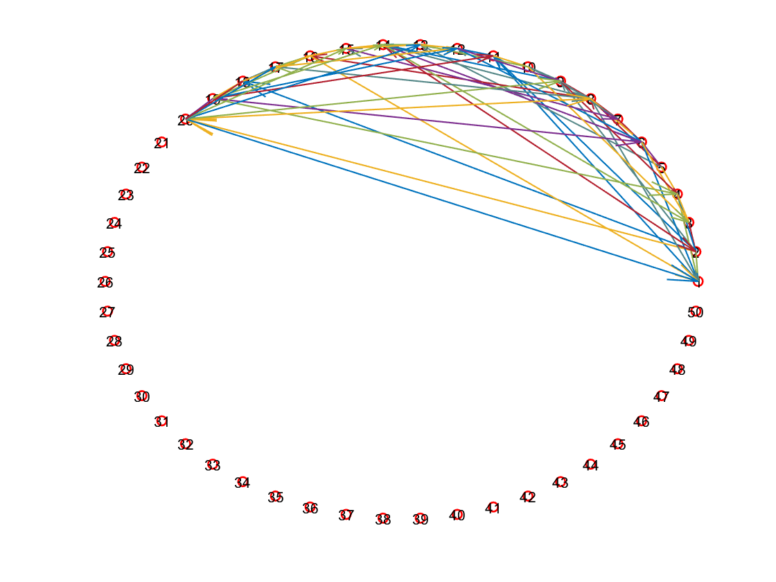
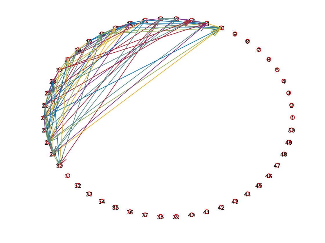
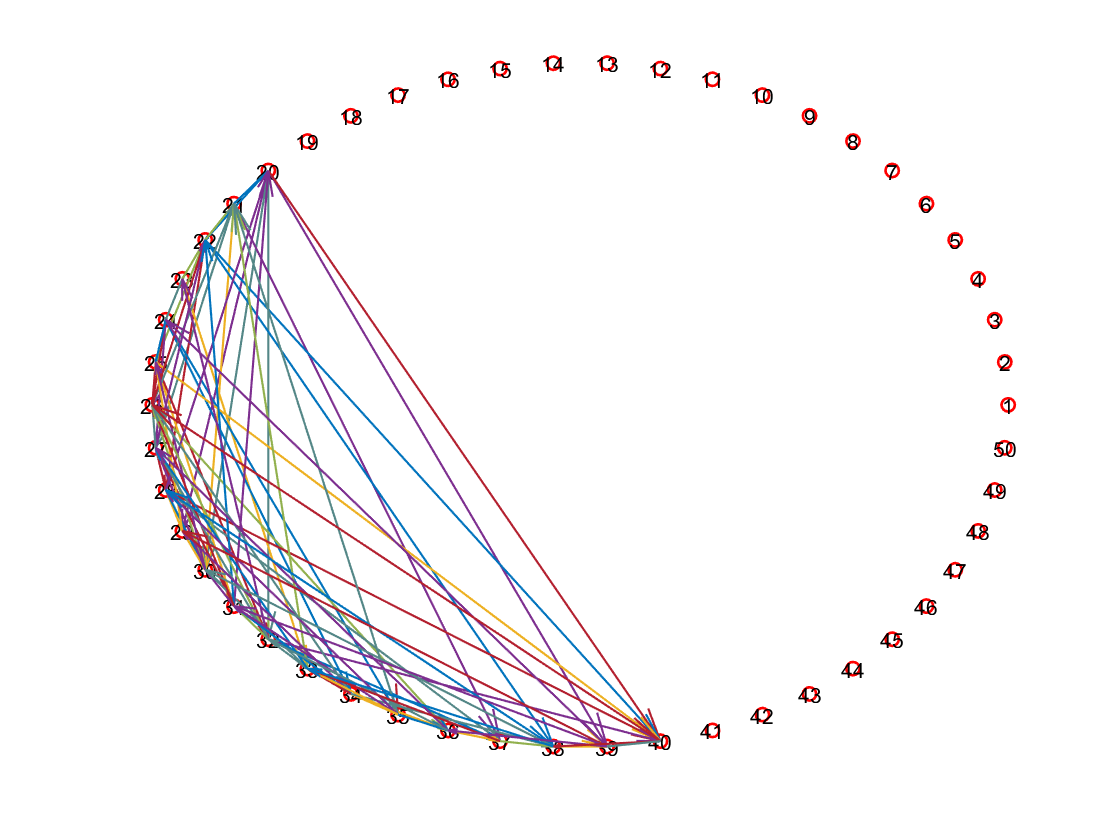
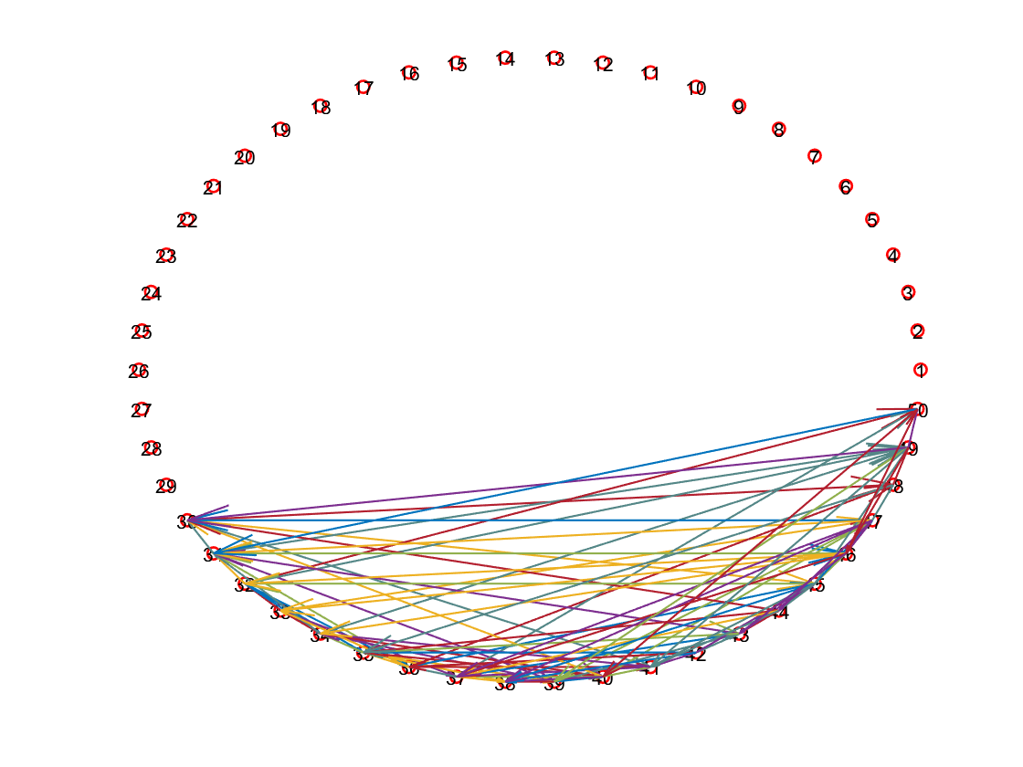
Figure 1: Schematic illustration of four switching graphs.

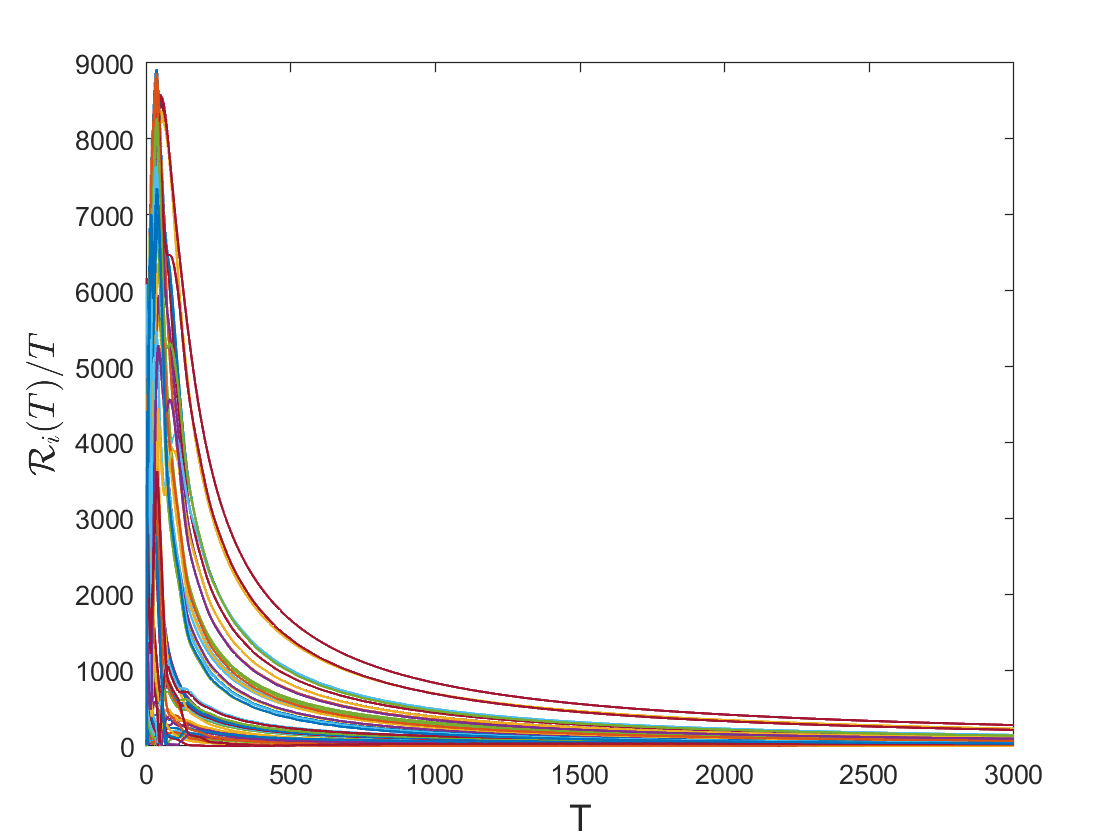
Figure 2: The trajectories of $\mathcal{R}_{i}$, $i\in[N]$.

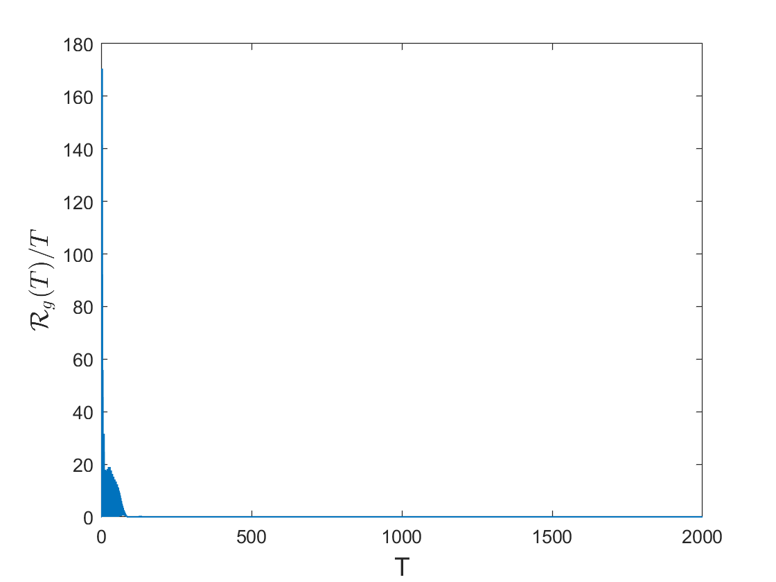
Figure 3: The trajectories of $\mathcal{R}_{g}$.

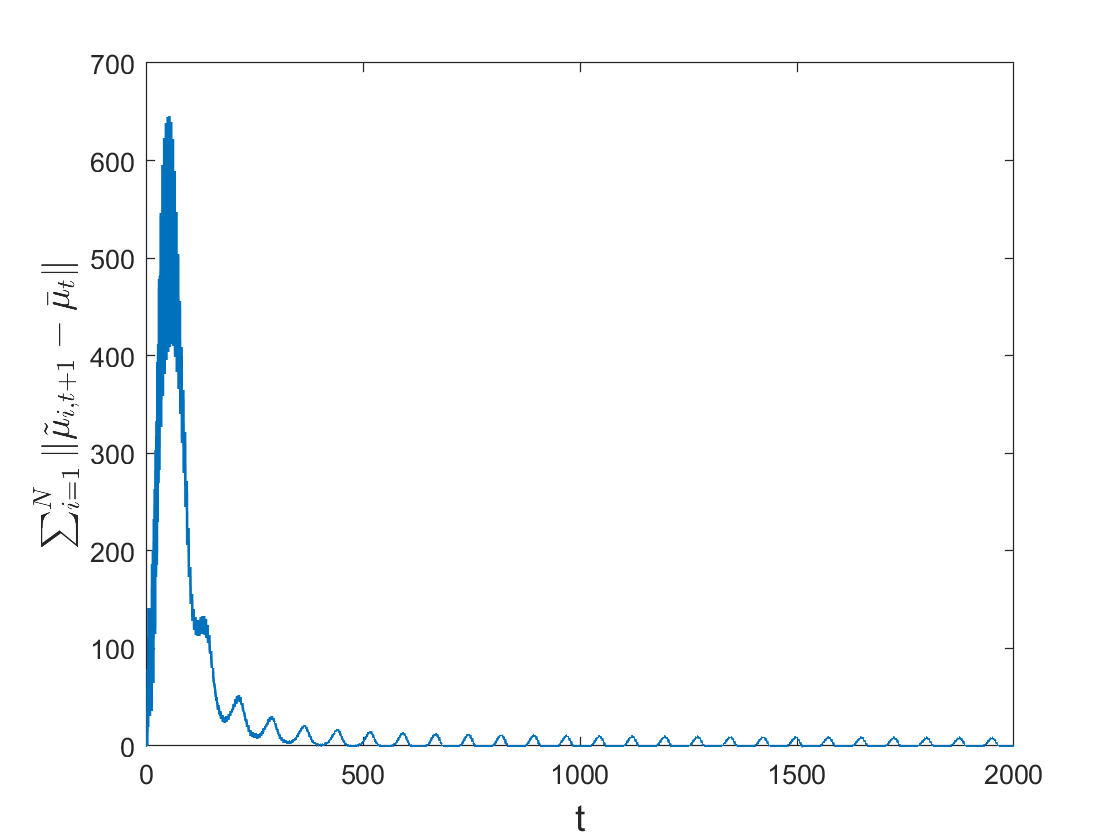
Figure 4: The trajectory of $\sum_{i=1}^{N}\|\tilde{\mu}_{i,t+1}-\bar{\mu}_{t}\|$.

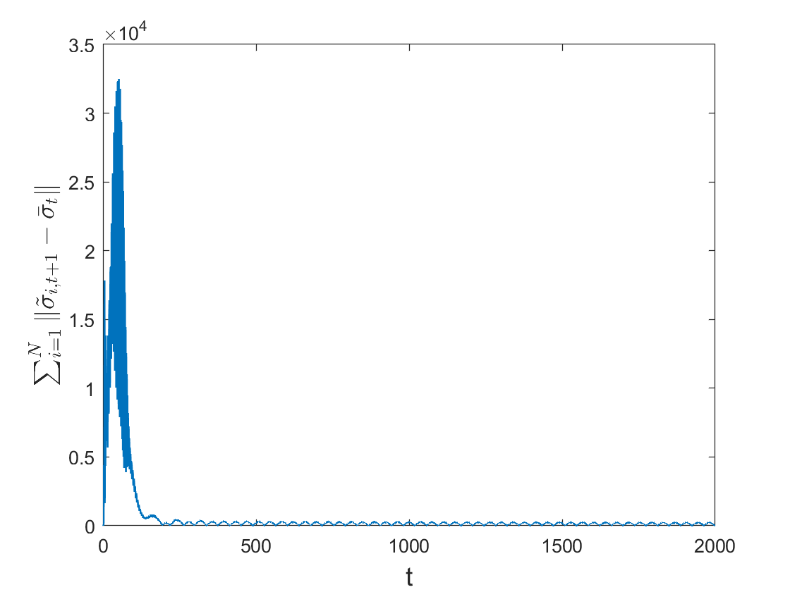
Figure 5: The trajectory of $\sum_{i=1}^{N}\|\tilde{\sigma}_{i,t+1}-\bar{\sigma}_{t}\|$.

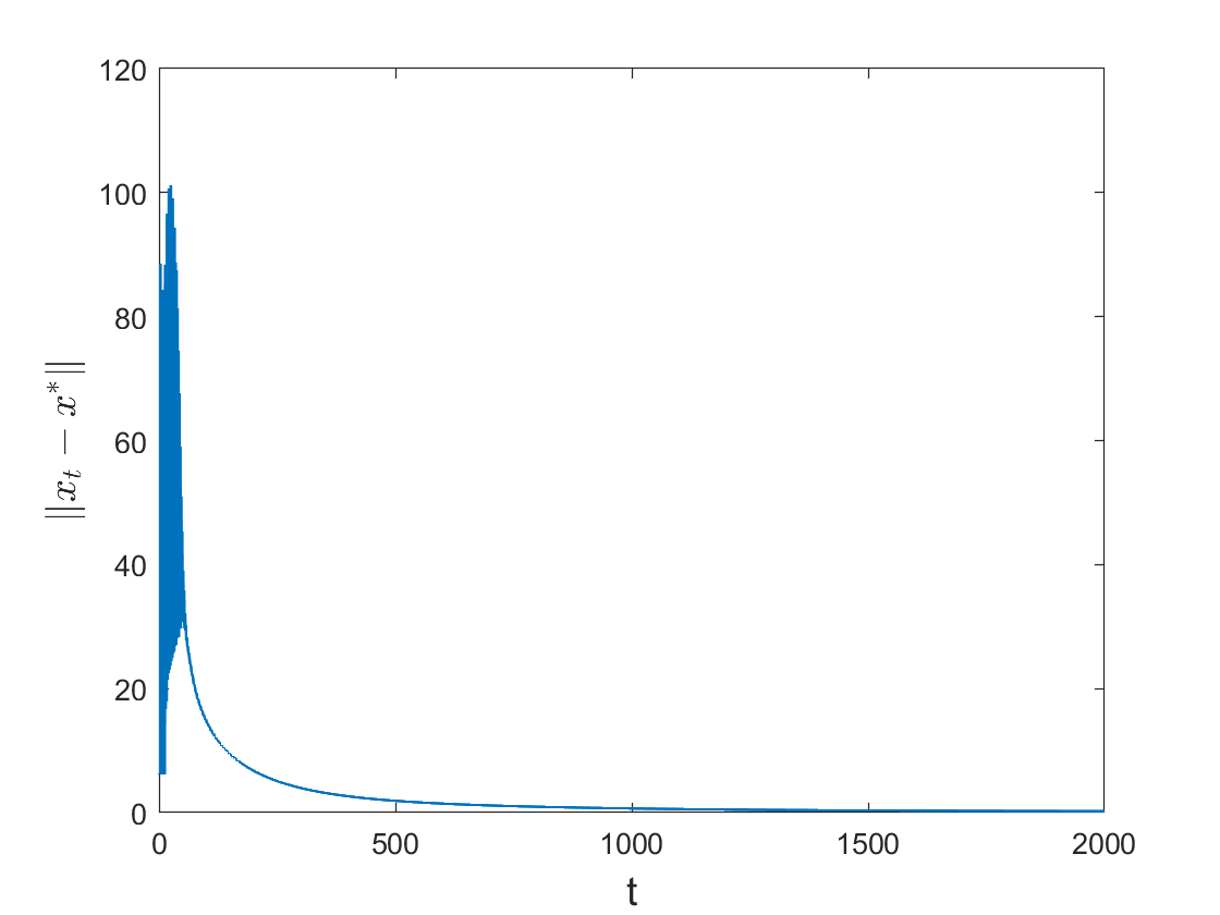
Figure 6: The trajectory of $\|x_{t}-x^{*}\|$.

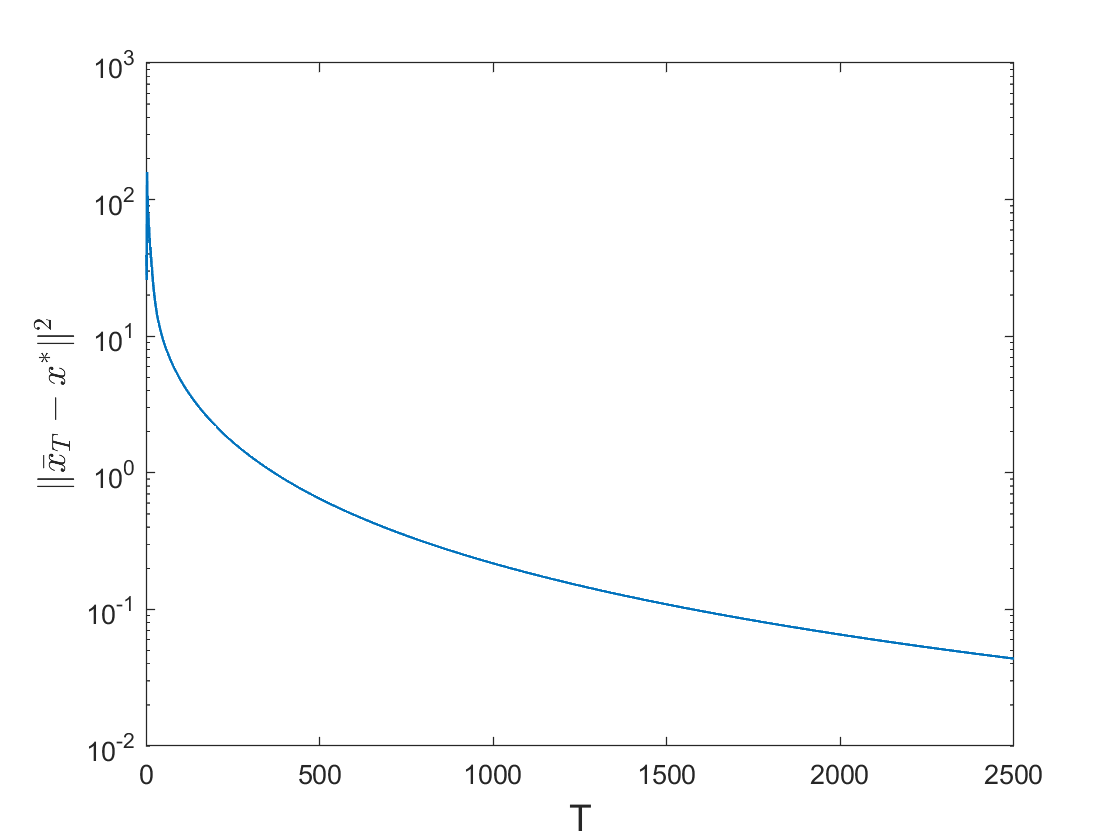
Figure 7: The trajectory of $\|\bar{x}_{T}-x^{*}\|^{2}$.

V CONCLUSION

In this paper, distributed learning for stochastic online aggregative games satisfying local set constraints and time-varying general convex constraints was studied for the first time. An online distributed stochastic primal-dual push-sum algorithm was devised, which is applicable to the unbalanced networks. It was rigorously shown that the regrets and constraint violation increase sublinearly with high probability by utilizing the sub-Gaussian noise model. In addition, in the offline case, the developed algorithm was proved to almost surely converge to the VGNE for strongly monotone games, and the high probability convergence rate of the time-averaged decision sequence was also analyzed. The algorithm’s performance was validated by a numerical application. Future work may focus on nonconvex cost functions.

Appendix A Proof of Lemma 1

Proof.

The proof of (14) can be found in Lemma 3 of [39]. Next, we derive (15) by mathematical induction. Due to the fact that $\mu_{i,0}=0$, $\forall i\in[N]$, it is obvious that $\hat{\mu}_{i,0}\leq\frac{z_{i,1}L}{\beta_{0}r^{2}}$, $\forall i\in[N]$. Assume that (15) holds for any time $t$ and $i\in[N]$. We show that it still holds at time $t+1$. To begin with, one can obtain

$$\|\mu_{i,t+1}\| \leq(1-\gamma_{t}\beta_{t})\|\hat{\mu}_{i,t}\|+\gamma_{t}\|g_{i,t}(x_{i,t})\|$$

$$\leq(1-\gamma_{t}\beta_{t})\frac{z_{i,t+1}L}{\beta_{t}r^{2}}+\frac{\gamma_{t}L}{r}$$

$$=\left(1-\gamma_{t}\beta_{t}+\frac{\gamma_{t}\beta_{t}r}{z_{i,t+1}}\right)\frac{z_{i,t+1}L}{\beta_{t}r^{2}}$$

$$\leq\frac{z_{i,t+1}L}{\beta_{t}r^{2}},$$

where $r\leq 1$ has been utilized in the first inequality and the last inequality is due to $z_{i,t+1}\geq r$. Hence, it further yields that

$$\|\hat{\mu}_{i,t+1}\| =\sum_{j=1}^{N}w_{ij,t+1}\mu_{j,t+1}$$

$$\leq\frac{L}{\beta_{t}r^{2}}\sum_{j=1}^{N}w_{ij,t+1}z_{j,t+1}$$

$$\leq\frac{w_{i,t+2}L}{\beta_{t+1}r^{2}},$$

where $\beta_{t+1}\leq\beta_{t}$ and (13a) have been employed to obtain the last inequality.

Note that $\hat{\mu}_{i,t}=\sum_{j=1}^{N}w_{ij,t}\mu_{j,t}\geq w_{ii,t}\mu_{i,t}$, by virtue of $w_{ii,t}\geq w$ from Assumption 1-i), one can obtain $\|\mu_{i,t}\|\leq\frac{\hat{\mu}_{i,t}}{w_{ii,t}}\leq\frac{z_{i,t+1}L}{\beta_{t}r^{2}w}$. The proof is ended. ∎

Appendix B Proof of Lemma 2

Proof.

It follows directly from Lemma 1 in [30] that

$$\|\tilde{\mu}_{i,t+1}-\bar{\mu}_{t}\|\leq\frac{8}{r}\left(\vartheta^{t}\|\mu_{0}\|_{1}+\sum_{k=1}^{t}\vartheta^{t-k}\|\varepsilon_{\mu_{k}}\|_{1}\right),$$

where $\varepsilon_{\mu_{k}}:=\operatorname*{col}\{\varepsilon_{\mu_{i,k}}\}_{i\in[N]}$ and $\mu_{0}:=\operatorname*{col}\{\mu_{i,0}\}_{i\in[N]}$. For the term $\|\varepsilon_{\mu_{k}}\|_{1}$, one has

$$\|\varepsilon_{\mu_{i,k}}\|_{1} \leq\sqrt{m}\|\varepsilon_{\mu_{i,k}}\|$$

$$\leq\gamma_{k-1}\sqrt{m}\|g_{i,k-1}(x_{i,k-1})-\beta_{k-1}\hat{\mu}_{i,k-1}\|$$

$$\leq 2\gamma_{k-1}\sqrt{m}L,$$

where the relation $\|a\|_{1}\leq\sqrt{p}\|a\|$ for $a\in\mathbb{R}^{p}$ has been employed in the first inequality, the second inequality is derived from (3) and Lemma 1. Hence, in view of $\|\varepsilon_{\mu_{k}}\|_{1}=\sum_{i=1}^{N}\|\varepsilon_{\mu_{i,k}}\|_{1}$ and $\mu_{i,0}=0$, $i\in[N]$, (20) holds.

Again using Lemma 1 in [30], it gives

$$\|\tilde{\sigma}_{i,t+1}-\bar{\sigma}_{t}\|\leq\frac{8}{r}\left(\vartheta^{t}\|\sigma_{0}\|_{1}+\sum_{k=1}^{t}\vartheta^{t-k}\|\varepsilon_{\sigma_{k}}\|_{1}\right),$$

where $\varepsilon_{\sigma_{k}}:=\operatorname*{col}\{\varepsilon_{\sigma_{i,k}}\}_{i\in[N]}$ and $\sigma_{0}:=\operatorname*{col}\{\sigma_{i,0}\}_{i\in[N]}$. Note that

$$\|\varepsilon_{\sigma_{i,k}}\|_{1} \leq\sqrt{n}\|\varepsilon_{\sigma_{i,k}}\|$$

$$\leq L_{\sigma}\sqrt{n}\|x_{i,k}-x_{i,k-1}\|$$

$$\leq\alpha_{k-1}L_{\sigma}\sqrt{n}\|s_{i,k}\|$$

$$\leq\alpha_{k-1}L_{\sigma}\sqrt{n}\left(S+\frac{LM}{\beta_{k-1}r^{2}}\right),$$

where the second inequality applies Assumption 2-v), the third inequality holds due to (13d), and the last inequality is obtained based on (13c), Assumptions 3, 4-iii), and (15) in Lemma 1. Hence, (21) can be derived, which ends the proof. ∎

Appendix C Proof of Lemma 3

Proof.

In view of the exponential inequality $\exp(a)\leq\exp(a^{2})+a$ for any $a\in\mathbb{R}$ and invoking $\|x_{i,t}-x_{i}\|^{2}\leq 4L^{2}$ by (3) one has

$$\exp(\alpha_{t}\langle\Delta_{t},x_{i,t}-x_{i}\rangle)$$

$$\leq\exp(4L^{2}\alpha_{t}^{2}\|\Delta_{t}\|^{2})+\alpha_{t}\langle\Delta_{t},x_{i,t}-x_{i}\rangle.$$

Taking conditional expectation with respect to $\mathscr{F}_{t}$ from both sides of the above inequality, it derives that

$$\mathrm{E}\left[\exp\left(\frac{\alpha_{t}}{2L\iota}\langle\Delta_{t},x_{i,t}-x_{i}\rangle\right)\bigg{|}\mathscr{F}_{t}\right]$$

$$\leq\mathrm{E}\left[\exp(\alpha_{t}^{2}\|\Delta_{t}\|^{2}/\iota^{2})|\mathscr{F}_{t}\right]$$

$$\leq\left(\mathrm{E}[\exp(\|\Delta_{t}\|^{2}/\iota^{2})|\mathscr{F}_{t}]\right)^{\alpha_{t}^{2}}$$

$$\leq\exp(\alpha_{t}^{2}),$$ (40)

where the first inequality holds since $\mathrm{E}[\langle\Delta_{t},x_{i,t}-x_{i}\rangle|\mathscr{F}_{t}]=\mathrm{E}[\Delta_{t}^{\textit{T}}|\mathscr{F}_{t}](x_{i,t}-x_{i})=0$ by Assumption 4-i), the second inequality holds by leveraging Jensen’s inequality and the fact that $\alpha_{t}\in[0,1]$, and the last inequality is based on Assumption 4-ii). Next, define $v_{i,t}:=\frac{\alpha_{t}}{2L\iota}\langle\Delta_{t},x_{i,t}-x_{i}\rangle)$ and consider the dynamics $u_{i,t+1}=\exp(v_{i,t}-\alpha_{t}^{2})u_{i,t}$ with $u_{i,1}=1$. Then it can be observed that $u_{i,t+1}=\exp(\sum_{l=1}^{t}(v_{i,l}-\alpha_{l}^{2}))$. Furthermore, it follows from (C) that $\mathrm{E}[u_{i,t+1}|\mathscr{F}_{t}]=\mathrm{E}[\exp(v_{i,t}-\alpha_{t}^{2})u_{i,t}|\mathscr{F}_{t}]\leq u_{i,t}$. Taking full expectation leads to that

$$\mathrm{E}[u_{i,t+1}]\leq\mathrm{E}[u_{i,t}]\leq\cdots\leq u_{i,1}=1.$$ (41)

Note that for any $\kappa>0$, it has

$$\mathrm{P}\left[\sum_{t=1}^{T}(v_{i,t}-\alpha_{t}^{2})\geq\kappa\right]$$

$$=\mathrm{P}\left[\exp\left(\sum_{t=1}^{T}(v_{i,t}-\alpha_{t}^{2})\right)\geq\exp(\kappa)\right]$$

$$=\mathrm{P}[u_{i,t+1}\geq\exp(\kappa)]$$

$$\leq\frac{\mathrm{E}[u_{i,t+1}]}{\exp(\kappa)}$$

$$\leq\exp(-\kappa),$$

where the first inequality holds owing to Markov’s inequality, and the last inequality is derived based on (41). Letting $\kappa=\ln\frac{1}{\delta}$ with $0<\delta<1$, it yields that with probability at least $1-\delta$,

$$\sum_{t=1}^{T}\alpha_{t}\langle\Delta_{t},x_{i,t}-x_{i}\rangle\leq 2L\iota\sum_{t=1}^{T}\alpha_{t}^{2}+2L\iota\ln\frac{1}{\delta}.$$

The proof is ended. ∎

Appendix D Proof of Lemma 4

Proof.

It follow from (13d) and (2) that for $x_{i}\in X_{i}$,

$$\langle x_{i,t}-\alpha_{t}s_{i,t+1}-x_{i,t+1},x_{i}-x_{i,t+1}\rangle\leq 0.$$ (42)

Hence

$$\alpha_{t}\langle x_{i,t+1}-x_{i},s_{i,t+1}\rangle$$

$$\leq\langle x_{i,t}-x_{i,t+1},x_{i,t+1}-x_{i,t}\rangle$$

$$=\frac{1}{2}(\|x_{i,t}-x_{i}\|^{2}-\|x_{i,t+1}-x_{i}\|^{2}-\|x_{i,t+1}-x_{i,t}\|^{2}).$$ (43)

Note that

$$\alpha_{t}\langle x_{i}-x_{i,t+1},\nabla g_{i,t}(x_{i,t})\tilde{\mu}_{i,t+1}\rangle$$

$$=\alpha_{t}(x_{i}-x_{i,t})^{\textit{T}}\nabla g_{i,t}(x_{i,t})\tilde{\mu}_{i,t+1}$$

$$\quad+\alpha_{t}(x_{i,t}-x_{i,t+1})^{\textit{T}}\nabla g_{i,t}\left(x_{i,t}\right)\tilde{\mu}_{i,t+1}$$

$$\leq\alpha_{t}\tilde{\mu}_{i,t+1}^{\textit{T}}(g_{i,t}(x_{i})-g_{i,t}(x_{i,t}))$$

$$\quad+\alpha_{t}(x_{i,t}-x_{i,t+1})^{\textit{T}}\nabla g_{i,t}(x_{i,t})\tilde{\mu}_{i,t+1}$$

$$=\alpha_{t}(\tilde{\mu}_{i,t+1}-\bar{\mu}_{t})^{\textit{T}}(g_{i,t}(x_{i})-g_{i,t}(x_{i,t}))$$

$$\quad+\alpha_{t}\bar{\mu}_{t}^{\textit{T}}(g_{i,t}(x_{i})-g_{i,t}(x_{i,t}))$$

$$\quad+\alpha_{t}(x_{i,t}-x_{i,t+1})^{\textit{T}}\nabla g_{i,t}(x_{i,t})\tilde{\mu}_{i,t+1}$$

$$\leq 2L\alpha_{t}\|\tilde{\mu}_{i,t+1}-\bar{\mu}_{t}\|+\alpha_{t}\bar{\mu}_{t}^{\textit{T}}(g_{i,t}(x_{i})-g_{i,t}(x_{i,t}))$$

$$\quad+\frac{1}{4}\|x_{i,t}-x_{i,t+1}\|^{2}+\alpha_{t}^{2}\|\nabla g_{i,t}(x_{i,t})\|^{2}\|\tilde{\mu}_{i,t+1}\|^{2}$$

$$\leq\frac{32L^{2}N\sqrt{m}}{r}\alpha_{t}\sum_{k=1}^{t}\vartheta^{t-k}\gamma_{k-1}+\alpha_{t}\bar{\mu}_{t}^{\textit{T}}(g_{i,t}(x_{i})-g_{i,t}(x_{i,t})$$

$$\quad+\frac{1}{4}\|x_{i,t}-x_{i,t+1}\|^{2}+\frac{M^{2}L^{2}}{r^{4}}\frac{\alpha_{t}^{2}}{\beta_{t}^{2}},$$ (44)

where the first inequality is obtained by using the convexity of $g_{ij,t}$ from Assumption 2-iii) and $\tilde{\mu}_{i,t+1}\geq{\bf 0}$, the second inequality is derived by (3), the Young’s inequality and Cauchy-Schwartz inequality, and the last inequality holds based on (20) in Lemma 2, (15) in Lemma 1, and Assumption 2-iv). Then it can be derived from (D) and (D) that

$$\alpha_{t}\langle x_{i,t+1}-x_{i},q_{i,t}(x_{i,t},\tilde{\sigma}_{i,t+1},\xi_{i,t})\rangle$$

$$\leq\langle x_{i,t}-x_{i,t+1},x_{i,t+1}-x_{i,t}\rangle$$

$$\quad+\alpha_{t}\langle x_{i}-x_{i,t+1},\nabla g_{i,t}(x_{i,t})\tilde{\mu}_{i,t+1}\rangle$$

$$=\frac{1}{2}(\|x_{i,t}-x_{i}\|^{2}-\|x_{i,t+1}-x_{i}\|^{2}-\|x_{i,t+1}-x_{i,t}\|^{2})$$

$$\quad+\alpha_{t}\langle x_{i}-x_{i,t+1},\nabla g_{i,t}(x_{i,t})\tilde{\mu}_{i,t+1}\rangle$$

$$\leq\frac{1}{2}\|x_{i,t}-x_{i}\|^{2}-\frac{1}{2}\|x_{i,t+1}-x_{i}\|^{2}-\frac{1}{4}\|x_{i,t+1}-x_{i,t}\|^{2}$$

$$\quad+\frac{32L^{2}N\sqrt{m}}{r}\alpha_{t}\sum_{k=1}^{t}\vartheta^{t-k}\gamma_{k-1}$$

$$\quad+\alpha_{t}\bar{\mu}_{t}^{\textit{T}}(g_{i,t}(x_{i})-g_{i,t}(x_{i,t})+\frac{M^{2}L^{2}}{r^{4}}\frac{\alpha_{t}^{2}}{\beta_{t}^{2}}.$$ (45)

Hence

$$\alpha_{t}\langle p_{i,t}(x_{i,t},\sigma(x_{t})),x_{i,t}-x_{i}\rangle$$

$$=\alpha_{t}\langle p_{i,t}(x_{i,t},\sigma(x_{t}))-p_{i,t}(x_{i,t},\tilde{\sigma}_{i,t+1})),x_{i,t}-x_{i}\rangle$$

$$\quad+\alpha_{t}\langle q_{i,t}(x_{i,t},\tilde{\sigma}_{i,t+1},\xi_{i,t}),x_{i,t}-x_{i,t+1}\rangle$$

$$\quad+\alpha_{t}\langle\Delta_{t},x_{i,t}-x_{i}\rangle+\alpha_{t}\langle q_{i,t}(x_{i,t},\tilde{\sigma}_{i,t+1},\xi_{i,t}),x_{i,t+1}-x_{i}\rangle$$

$$\leq\alpha_{t}\|p_{i,t}(x_{i,t},\sigma(x_{t}))-p_{i,t}(x_{i,t},\tilde{\sigma}_{i,t+1}))\|\|x_{i,t}-x_{i}\|$$

$$\quad+\frac{1}{4}\|x_{i,t+1}-x_{i,t}\|^{2}+\alpha_{t}^{2}\|q_{i,t}(x_{i,t},\tilde{\sigma}_{i,t+1},\xi_{i,t})\|^{2}$$

$$\quad+\alpha_{t}\langle\Delta_{t},x_{i,t}-x_{i}\rangle+\alpha_{t}\langle q_{i,t}(x_{i,t},\tilde{\sigma}_{i,t+1},\xi_{i,t}),x_{i,t+1}-x_{i}\rangle$$

$$\leq 2Ll_{f}\alpha_{t}\|\sigma(x_{t})-\tilde{\sigma}_{i,t+1}\|+\frac{1}{4}\|x_{i,t+1}-x_{i,t}\|^{2}+S^{2}\alpha_{t}^{2}$$

$$\quad+\alpha_{t}\langle\Delta_{t},x_{i,t}-x_{i}\rangle+\alpha_{t}\langle q_{i,t}(x_{i,t},\tilde{\sigma}_{i,t+1},\xi_{i,t}),x_{i,t+1}-x_{i}\rangle$$

$$\leq S^{2}\alpha_{t}^{2}+\frac{16Ll_{f}}{r}\|\sigma_{0}\|_{1}\alpha_{t}\vartheta^{t}+\frac{32L^{2}N\sqrt{m}}{r}\alpha_{t}\sum_{k=1}^{t}\vartheta^{t-k}\gamma_{k-1}$$

$$\quad+\frac{16LNSl_{f}\sqrt{n}L_{\sigma}}{r}\alpha_{t}\sum_{k=1}^{t}\vartheta^{t-k}\alpha_{k-1}$$

$$\quad+\frac{16N\sqrt{n}L_{\sigma}L^{2}l_{f}M}{r^{3}}\alpha_{t}\sum_{k=1}^{t}\vartheta^{t-k}\frac{\alpha_{k-1}}{\beta_{k-1}}$$

$$\quad+\alpha_{t}\langle\Delta_{t},x_{i,t}-x_{i}\rangle+\frac{1}{2}\|x_{i}-x_{i,t}\|^{2}-\frac{1}{2}\|x_{i}-x_{i,t+1}\|^{2}$$

$$\quad+\alpha_{t}\bar{\mu}_{t}^{\textit{T}}(g_{i,t}(x_{i})-g_{i,t}(x_{i,t}))+\frac{M^{2}L^{2}}{r^{4}}\frac{\alpha_{t}^{2}}{\beta_{t}^{2}},$$

where the first inequality results from the Cauchy-schwartz inequality and Young’s inequality, the second inequality utilizes Assumption 3, 4-iii), and (3), and the last inequality holds due to (D) and (21) in Lemma 2. Dividing $\alpha_{t}$ from both sides of the above inequality immediately yields assertion (4), which completes the proof. ∎

Appendix E Proof of Lemma 5

Proof.

It follows from (16) and (18) that

$$\bar{\mu}_{t+1}=\bar{\mu}_{t}+\frac{1}{N}\sum_{i=1}^{N}\varepsilon_{\mu_{i,t+1}}.$$ (46)

Hence, for any $\mu\in\mathbb{R}^{m}_{+}$, one has

$$\|\bar{\mu}_{t+1}-\mu\|^{2}$$

$$=\left\|\bar{\mu}_{t}-\mu+\frac{\sum_{i=1}^{N}\varepsilon_{\mu_{i,t+1}}}{N}\right\|^{2}$$

$$\leq\|\bar{\mu}_{t}-\mu\|^{2}+\frac{1}{N}\sum_{i=1}^{N}\|\varepsilon_{\mu_{i,t+1}}\|^{2}+\frac{2}{N}\sum_{i=1}^{N}\varepsilon_{\mu_{i,t+1}}^{\textit{T}}(\bar{\mu}_{t}-\mu)$$

$$\leq\|\bar{\mu}_{t}-\mu\|^{2}+\frac{\gamma_{t}^{2}}{N}\sum_{i=1}^{N}\|g_{i,t}(x_{i,t})-\beta_{t}\hat{\mu}_{i,t}\|^{2}$$

$$\quad+\frac{2}{N}\sum_{i=1}^{N}\varepsilon_{\mu_{i,t+1}}^{\textit{T}}(\bar{\mu}_{t}-\mu),$$ (47)

where the inequality $\|\sum_{i=1}^{s}a_{i}\|^{2}\leq s\sum_{i=1}^{s}\|a_{i}\|^{2}$ has been leveraged to obtain the first inequality, and the second inequality has utilized (1) and (18).

Next, let us deal with the last term in the last inequality of (E). It can be derived that

$$\varepsilon_{\mu_{i,t+1}}^{\textit{T}}(\bar{\mu}_{t}-\mu)$$

$$=\frac{1}{z_{i,t+1}}\varepsilon_{\mu_{i,t+1}}^{\textit{T}}(\hat{\mu}_{i,t}-z_{i,t+1}\mu)+\varepsilon_{\mu_{i,t+1}}^{\textit{T}}(\bar{\mu}_{t}-\tilde{\mu}_{i,t+1})$$

$$=(\varepsilon_{\mu_{i,t+1}}-\gamma_{t}(g_{i,t}(x_{i,t})-\beta_{t}\hat{\mu}_{i,t}))^{\textit{T}}\frac{\left(\hat{\mu}_{i,t}-w_{i,t+1}\mu\right)}{z_{i,t+1}}$$

$$\quad+\gamma_{t}(g_{i,t}(x_{i,t})-\beta_{t}\hat{\mu}_{i,t})^{\textit{T}}(\tilde{\mu}_{i,t+1}-\mu)$$

$$\quad+\varepsilon_{\mu_{i,t+1}}^{\textit{T}}(\bar{\mu}_{t}-\tilde{\mu}_{i,t+1})$$

$$=(\varepsilon_{\mu_{i,t+1}}-\gamma_{t}(g_{i,t}(x_{i,t})-\beta_{t}\hat{\mu}_{i,t}))^{\textit{T}}\frac{(\mu_{i,t+1}-z_{i,t+1}\mu)}{z_{i,t+1}}$$

$$\quad+(\varepsilon_{\mu_{i,t+1}}-\gamma_{t}(g_{i,t}(x_{i,t})-\beta_{t}\hat{\mu}_{i,t}))^{\textit{T}}\frac{(\hat{\mu}_{i,t}-\mu_{i,t+1})}{z_{i,t+1}}$$

$$\quad+\gamma_{t}(g_{i,t}(x_{i,t})-\beta_{t}\hat{\mu}_{i,t})^{\textit{T}}(\tilde{\mu}_{i,t+1}-\mu)$$

$$\quad+\varepsilon_{\mu_{i,t+1}}^{\textit{T}}(\bar{\mu}_{t}-\tilde{\mu}_{i,t+1})$$

$$\leq\frac{\gamma_{t}}{z_{i,t+1}}(g_{i,t}(x_{i,t})-\beta_{t}\hat{\mu}_{i,t})^{\textit{T}}(\mu_{i,t+1}-\hat{\mu}_{i,t})$$

$$\quad+\gamma_{t}(g_{i,t}(x_{i,t})-\beta_{t}\hat{\mu}_{i,t})^{\textit{T}}(\tilde{\mu}_{i,t+1}-\mu)$$

$$\quad+\varepsilon_{\mu_{i,t+1}}^{\textit{T}}(\bar{\mu}_{t}-\tilde{\mu}_{i,t+1})$$

$$\leq\frac{\gamma_{t}^{2}}{r}\|g_{i,t}(x_{i,t})-\beta_{t}\hat{\mu}_{i,t}\|^{2}$$

$$\quad+\gamma_{t}(g_{i,t}(x_{i,t})-\beta_{t}\hat{\mu}_{i,t})^{\textit{T}}(\tilde{\mu}_{i,t+1}-\mu)$$

$$\quad+\gamma_{t}\|g_{i,t}(x_{i,t})-\beta_{t}\hat{\mu}_{i,t}\|\|\tilde{\mu}_{i,t+1}-\bar{\mu}_{t}\|,$$

where the first inequality is obtained by (2), and the lat inequality is derived by utilizing the Cauchy–Schwartz inequality, (14) in Lemma 1, (13e), and (1).

Then substituting the inequality above into (E) leads to

$$\|\bar{\mu}_{t+1}-\mu\|^{2}$$

$$\leq\|\bar{\mu}_{t}-\mu\|^{2}+\left(1+\frac{2}{r}\right)\frac{\gamma_{t}^{2}}{N}\sum_{i=1}^{N}\|g_{i,t}(x_{i,t})-\beta_{t}\hat{\mu}_{i,t}\|^{2}$$

$$\quad+\frac{2\gamma_{t}}{N}\sum_{i=1}^{N}g_{i,t}(x_{i,t})^{\textit{T}}(\tilde{\mu}_{i,t+1}-\mu)$$

$$\quad-\frac{\gamma_{t}\beta_{t}}{N}\sum_{i=1}^{N}2\hat{\mu}_{i,t}^{\textit{T}}(\tilde{\mu}_{i,t+1}-\mu)$$

$$\quad+\frac{2\gamma_{t}}{N}\sum_{i=1}^{N}\|g_{i,t}(x_{i,t})-\beta_{t}\hat{\mu}_{i,t}\|\|\tilde{\mu}_{i,t+1}-\bar{\mu}_{t}\|.$$ (48)

For the second term on the right of (E), by (3) and (14) in Lemma 1, one has

$$\|g_{i,t}(x_{i,t})-\beta_{t}\hat{\mu}_{i,t}\|^{2} \leq 2\|g_{i,t}(x_{i,t})\|^{2}+2\|\beta_{t}\hat{\mu}_{i,t}\|^{2}$$

$$\leq 2L^{2}+\frac{2L^{2}N^{2}}{r^{4}}.$$ (49)

Regarding the third term on the right of (E), it can be derived from (3) that

$$g_{i,t}(x_{i,t})^{\textit{T}}(\tilde{\mu}_{i,t+1}-\mu)$$

$$=g_{i,t}(x_{i,t})^{\textit{T}}(\tilde{\mu}_{i,t+1}-\bar{\mu}_{t})+g_{i,t}(x_{i,t})^{\textit{T}}(\bar{\mu}_{t}-\mu)$$

$$\leq L\|\tilde{\mu}_{i,t+1}-\bar{\mu}_{t}\|+g_{i,t}(x_{i,t})^{\textit{T}}(\bar{\mu}_{t}-\mu).$$ (50)

As for the fourth term on the right of (E), invoking Lemma 1, one can obtain

$$-2\hat{\mu}_{i,t}^{\textit{T}}(\tilde{\mu}_{i,t+1}-\mu) =-2z_{i,t+1}\tilde{\mu}_{i,t+1}(\tilde{\mu}_{i,t+1}-\mu)$$

$$\leq z_{i,t+1}(\|\mu\|^{2}-\|\tilde{\mu}_{i,t+1}\|^{2})$$

$$\leq N\|\mu\|^{2}.$$ (51)

Substituting (E)-(E) and (20) in Lemma 2 into (E) gives rise to (5). Hence, the proof is completed. ∎

Appendix F Proof of Lemma 6

Proof.

Setting $x_{i}=x_{i}^{\star}$ in (4) in Lemma 4, it has

$$\langle p_{i,t}(x_{i,t},\sigma(x_{t})),x_{i,t}-x_{i}^{\star}\rangle$$

$$\leq S^{2}\alpha_{t}+\frac{16Ll_{f}}{r}\|\sigma_{0}\|_{1}\vartheta^{t}$$

$$\quad+\frac{16LNSl_{f}\sqrt{n}L_{\sigma}}{r}\sum_{k=1}^{t}\vartheta^{t-k}\alpha_{k-1}$$

$$\quad+\frac{16N\sqrt{n}L_{\sigma}L^{2}l_{f}M}{r^{3}}\sum_{k=1}^{t}\vartheta^{t-k}\frac{\alpha_{k-1}}{\beta_{k-1}}$$

$$\quad+\frac{32L^{2}N\sqrt{m}}{r}\sum_{k=1}^{t}\vartheta^{t-k}\gamma_{k-1}+\langle\Delta_{t},x_{i,t}-x_{i}^{\star}\rangle$$

$$\quad+\frac{1}{2\alpha_{t}}\|x_{i}^{\star}-x_{i,t}\|^{2}-\frac{1}{2\alpha_{t}}\|x_{i}^{\star}-x_{i,t+1}\|^{2}$$

$$\quad+\bar{\mu}_{t}^{\textit{T}}(g_{i,t}(x_{i}^{\star})-g_{i,t}(x_{i,t}))+\frac{M^{2}L^{2}}{r^{4}}\frac{\alpha_{t}}{\beta_{t}^{2}}.$$ (52)

Since $x_{i}^{\star}\in X_{i,t}(x_{-i,t})$, that is, $g_{i,t}(x_{i}^{\star})+\sum_{j\neq i,j=1}^{N}g_{j,t}(x_{j,t})\leq{\bf 0}$ and noting that $\bar{\mu}_{t}\geq{\bf 0}$, one can obtain that

$$\bar{\mu}_{t}^{\textit{T}}(g_{i,t}(x_{i}^{\star})-g_{i,t}(x_{i,t}))$$

$$=\bar{\mu}_{t}^{\textit{T}}\left(g_{i,t}(x_{i}^{\star})+\sum_{j\neq i,j=1}^{N}g_{j,t}(x_{j,t})-g_{t}(x_{t})\right)$$

$$\leq-\bar{\mu}_{t}^{\textit{T}}g_{t}(x_{t}).$$ (53)

Substituting (F) into (F) results in

$$\langle p_{i,t}(x_{i,t},\sigma(x_{t})),x_{i,t}-x_{i}^{\star}\rangle$$

$$\leq S^{2}\alpha_{t}+\frac{16Ll_{f}}{r}\|\sigma_{0}\|_{1}\vartheta^{t}$$

$$\quad+\frac{16LNSl_{f}\sqrt{n}L_{\sigma}}{r}\sum_{k=1}^{t}\vartheta^{t-k}\alpha_{k-1}$$

$$\quad+\frac{16N\sqrt{n}L_{\sigma}L^{2}l_{f}M}{r^{3}}\sum_{k=1}^{t}\vartheta^{t-k}\frac{\alpha_{k-1}}{\beta_{k-1}}$$

$$\quad+\frac{32L^{2}N\sqrt{m}}{r}\sum_{k=1}^{t}\vartheta^{t-k}\gamma_{k-1}-\bar{\mu}_{t}^{\textit{T}}g_{t}(x_{t})$$

$$\quad+\frac{M^{2}L^{2}}{r^{4}}\frac{\alpha_{t}}{\beta_{t}^{2}}+\langle\Delta_{t},x_{i,t}-x_{i}^{\star}\rangle$$

$$\quad+\frac{1}{2\alpha_{t}}\|x_{i}^{\star}-x_{i,t}\|^{2}-\frac{1}{2\alpha_{t}}\|x_{i}^{\star}-x_{i,t+1}\|^{2}.$$ (54)

Dividing both sides of (5) by $\frac{2\gamma_{t}}{N}$, one can obtain

$$\frac{N}{2\gamma_{t}}\|\bar{\mu}_{t+1}-\mu\|^{2}$$

$$\leq\frac{N}{2\gamma_{t}}\|\bar{\mu}_{t}-\mu\|^{2}+\left(1+\frac{2}{r}\right)\left(1+\frac{N^{2}}{r^{4}}\right)NL^{2}\gamma_{t}$$

$$\quad+\frac{16N^{2}\sqrt{m}L^{2}}{r}\left(2+\frac{N}{r^{2}}\right)\sum_{k=1}^{t}\vartheta^{t-k}\gamma_{k-1}$$

$$\quad+g_{t}(x_{t})^{\textit{T}}(\bar{\mu}_{t}-\mu)+\frac{N^{2}}{2}\beta_{t}\|\mu\|^{2}.$$ (55)

Then combining (F) and (F) yields that

$$\langle p_{i,t}(x_{i,t},\sigma(x_{t})),x_{i,t}-x_{i}^{\star}\rangle$$

$$\leq S^{2}\alpha_{t}+\frac{16Ll_{f}}{r}\|\sigma_{0}\|_{1}\vartheta^{t}-\mu^{\textit{T}}g_{t}(x_{t})+\langle\Delta_{t},x_{i,t}-x_{i}^{\star}\rangle$$

$$\quad+\frac{16LNSl_{f}\sqrt{n}L_{\sigma}}{r}\sum_{k=1}^{t}\vartheta^{t-k}\alpha_{k-1}$$

$$\quad+\frac{16N\sqrt{n}L_{\sigma}L^{2}l_{f}M}{r^{3}}\sum_{k=1}^{t}\vartheta^{t-k}\frac{\alpha_{k-1}}{\beta_{k-1}}+\frac{M^{2}L^{2}}{r^{4}}\frac{\alpha_{t}}{\beta_{t}^{2}}$$

$$\quad+\frac{1}{2\alpha_{t}}\|x_{i}^{\star}-x_{i,t}\|^{2}-\frac{1}{2\alpha_{t}}\|x_{i}^{\star}-x_{i,t+1}\|^{2}$$

$$\quad-\mu^{\textit{T}}g_{t}(x_{t})+\frac{N^{2}}{2}\beta_{t}\|\mu\|^{2}+\left(1+\frac{2}{r}\right)\left(1+\frac{N^{2}}{r^{4}}\right)NL^{2}\gamma_{t}$$

$$\quad+\frac{16N\sqrt{m}L^{2}}{r}\left(2(N+1)+\frac{N^{2}}{r^{2}}\right)\sum_{k=1}^{t}\vartheta^{t-k}\gamma_{k-1}$$

$$\quad+\frac{N}{2\gamma_{t}}\|\bar{\mu}_{t}-\mu\|^{2}-\frac{N}{2\gamma_{t}}\|\bar{\mu}_{t+1}-\mu\|^{2}.$$ (56)

Summing over $t=1,\ldots,T$ from both sides of (F), it is straightforward to obtain that

$$\sum_{t=1}^{T}\langle p_{i,t}(x_{i,t},\sigma(x_{t})),x_{i,t}-x_{i}^{\star}\rangle$$

$$\leq S^{2}\sum_{t=1}^{T}\alpha_{t}+\frac{16Ll_{f}}{r}\|\sigma_{0}\|_{1}\sum_{t=1}^{T}\vartheta^{t}+\sum_{t=1}^{T}\langle\Delta_{t},x_{i,t}-x_{i}^{\star}\rangle$$

$$\quad+\sum_{t=1}^{T}\frac{1}{2\alpha_{t}}(\|x_{i}^{\star}-x_{i,t}\|^{2}-\|x_{i}^{\star}-x_{i,t+1}\|^{2})$$

$$\quad+\left(1+\frac{2}{r}\right)\left(1+\frac{N^{2}}{r^{4}}\right)NL^{2}\sum_{t=1}^{T}\gamma_{t}$$

$$\quad+\frac{16LNSl_{f}\sqrt{n}L_{\sigma}}{r}\sum_{t=1}^{T}\sum_{k=1}^{t}\vartheta^{t-k}\alpha_{k-1}$$

$$\quad+\frac{16N\sqrt{n}L_{\sigma}L^{2}l_{f}M}{r^{3}}\sum_{t=1}^{T}\sum_{k=1}^{t}\vartheta^{t-k}\frac{\alpha_{k-1}}{\beta_{k-1}}$$

$$\quad+\frac{16N\sqrt{m}L^{2}}{r}\left(2(N+1)+\frac{N^{2}}{r^{2}}\right)\sum_{t=1}^{T}\sum_{k=1}^{t}\vartheta^{t-k}\gamma_{k-1}$$

$$\quad-\mu^{\textit{T}}\sum_{t=1}^{T}g_{t}(x_{t})+\frac{N^{2}}{2}\|\mu\|^{2}\sum_{t=1}^{T}\beta_{t}+\frac{M^{2}L^{2}}{r^{4}}\sum_{t=1}^{T}\frac{\alpha_{t}}{\beta_{t}^{2}}$$

$$\quad+\sum_{t=1}^{T}\frac{N}{2\gamma_{t}}(\|\bar{\mu}_{t}-\mu\|^{2}-\|\bar{\mu}_{t+1}-\mu\|^{2}).$$ (57)

Note that

$$\sum_{t=1}^{T}\sum_{k=1}^{t}\vartheta^{t-k}\alpha_{k-1} =\sum_{t=0}^{T-1}\vartheta^{t}\sum_{k=0}^{T-t-1}\alpha_{k}$$

$$\leq\frac{1}{1-\vartheta}\sum_{t=0}^{T-1}\alpha_{t}.$$ (58)

Similarly, one has

$$\sum_{t=1}^{T}\sum_{k=1}^{t}\vartheta^{t-k}\frac{\alpha_{k-1}}{\beta_{k-1}}\leq\frac{1}{1-\vartheta}\sum_{t=0}^{T-1}\frac{\alpha_{t}}{\beta_{t}},$$

$$\sum_{t=1}^{T}\sum_{k=1}^{t}\vartheta^{t-k}\gamma_{k-1}\leq\frac{1}{1-\vartheta}\sum_{t=0}^{T-1}\gamma_{t}.$$ (59)

For the third term on the right of (F), in view of (3) in Lemma 3 and $\alpha_{t+1}\leq\alpha_{t}$, it can be obtained that with probability at least $1-\delta$,

$$\sum_{t=1}^{T}\langle\Delta_{t},x_{i,t}-x_{i}^{\star}\rangle\leq\frac{2L\iota\sum_{t=1}^{T}\alpha_{t}^{2}}{\alpha_{T}}+\frac{2L\iota\ln\frac{1}{\delta}}{\alpha_{T}}.$$ (60)

For the fourth term on the right of (F), it derives that

$$\sum_{t=1}^{T}\frac{1}{2\alpha_{t}}(\|x_{i}^{\star}-x_{i,t}\|^{2}-\|x_{i}^{\star}-x_{i,t+1}\|^{2})$$

$$=\sum_{t=1}^{T}\left(\frac{1}{2\alpha_{t}}\|x_{i}^{\star}-x_{i,t}\|^{2}-\frac{1}{2\alpha_{t+1}}\|x_{i}^{\star}-x_{i,t+1}\|^{2}\right)$$

$$\quad+\sum_{t=1}^{T}\left(\frac{1}{2\alpha_{t+1}}-\frac{1}{2\alpha_{t}}\right)\|x_{i}^{\star}-x_{i,t+1}\|^{2}$$

$$\leq\frac{1}{\alpha_{1}}(\|x_{i}^{\star}\|^{2}+\|x_{i,1}\|^{2})$$

$$\quad+\sum_{t=1}^{T}\left(\frac{1}{\alpha_{t+1}}-\frac{1}{\alpha_{t}}\right)(\|x_{i}^{\star}\|^{2}+\|x_{i,t+1}\|^{2})$$

$$\leq\frac{2L^{2}}{\alpha_{T+1}},$$ (61)

where (3) has been used to get the last inequality.

Denote by $A(\mu):=\sum_{t=1}^{T}\frac{N}{2\gamma_{t}}(\|\bar{\mu}_{t}-\mu\|^{2}-\|\bar{\mu}_{t+1}-\mu\|^{2})$ and $B(\mu):=-\mu^{\textit{T}}\sum_{t=1}^{T}g_{t}(x_{t})+\frac{N^{2}}{2}\|\mu\|^{2}\sum_{t=1}^{T}\beta_{t}$. Following the same line as (F), one can obtain that

$$A({\bf 0}) =\sum_{t=1}^{T}\frac{N}{2\gamma_{t}}(\|\bar{\mu}_{t}\|^{2}-\|\bar{\mu}_{t+1}\|^{2})$$

$$\leq\frac{N\|\bar{\mu}_{1}\|^{2}}{2\gamma_{1}}+\sum_{t=1}^{T}\left(\frac{N}{2\gamma_{t+1}}-\frac{N}{2\gamma_{t}}\right)\|\bar{\mu}_{t+1}\|^{2}$$

$$\leq\frac{N^{2}L^{2}}{2r^{4}w^{2}\gamma_{T+1}\beta_{T+1}^{2}},$$ (62)

where we utilize $\|\bar{\mu}_{t}\|^{2}\leq\frac{1}{N}\|\mu_{i,t}\|^{2}\leq\frac{NL^{2}}{r^{4}w^{2}\beta_{t}^{2}}\leq\frac{NL^{2}}{r^{4}w^{2}\beta_{T+1}^{2}}$ by Lemma 1 to obtain the last inequality.

Note that

$$\mathcal{R}_{i}(T)\leq\sum_{t=1}^{T}\langle p_{i,t}(x_{i,t},\sigma(x_{t})),x_{i,t}-x_{i}^{\star}\rangle,$$

then substituting (F)-(F) into (F), and invoking $\alpha_{t}\leq\alpha_{t-1}$ and $\gamma_{t}\leq\gamma_{t-1}$, and $B({\bf 0})={\bf 0}$, assertion (25) can be obtained.

In addition, through a simple calculation, one can obtain that $B(\mu)$ achieves its minimal value $-\frac{\|[\sum_{t=1}^{T}g_{t}(x_{t})]_{+}\|^{2}}{2N^{2}\sum_{t=1}^{T}\beta_{t}}$ when $\mu=\mu_{0}:=\frac{[\sum_{t=1}^{T}g_{t}(x_{t})]_{+}}{N^{2}\sum_{t=1}^{T}\beta_{t}}$.

In view of (3), it obtains that $\|\mu_{0}\|\leq\frac{TL}{N\sum_{t=1}^{T}\beta_{t}}$. Hence, resorting to the similar argument as (F), it gives

$$A({\mu_{0}})\leq\frac{N^{2}L^{2}}{r^{4}w^{2}\gamma_{T+1}\beta_{T+1}^{2}}+\frac{T^{2}L^{2}}{N\gamma_{T+1}\left(\sum_{t=1}^{T}\beta_{t}\right)^{2}},$$ (63)

Incorporating (F)-(F) and (63), it can be concluded that

$$\sum_{t=1}^{T}\langle p_{i,t}(x_{i,t},\sigma(x_{t})),x_{i,t}-x_{i}^{\star}\rangle$$

$$\leq S_{1}(T)+S_{2}(T)+S_{5}(T)-\frac{\mathcal{R}^{2}_{g}(T)}{S_{4}(T)},$$

and thus by noting that $\langle p_{i,t}(x_{i,t},\sigma(x_{t})),x_{i,t}-x_{i}^{\star}\rangle\geq 0$, it holds

$$\mathcal{R}^{2}_{g}(T)\leq S_{4}(T)(S_{1}(T)+S_{2}(T)+S_{5}(T)).$$

The proof is ended.

∎

Appendix G Proof of Theorem 2

Proof.

Setting $x_{i}=x_{i}^{*}$ in (4) of Lemma 4, then summing over $i\in[N]$ and rearranging the terms, one can obtain

$$\|x_{t+1}-x^{*}\|^{2}$$

$$\leq\|x_{t}-x^{*}\|^{2}-2\alpha_{t}\sum_{i=1}^{N}\langle p_{i}(x_{i,t},\sigma(x_{t})),x_{i,t}-x_{i}^{*}\rangle$$

$$\quad+2\alpha_{t}\sum_{i=1}^{N}\langle\Delta_{t},x_{i,t}-x_{i}^{*}\rangle+2NS^{2}\alpha_{t}^{2}+\frac{32NLl_{f}}{r}\|\sigma_{0}\|_{1}\vartheta^{t}\alpha_{t}$$

$$\quad+\frac{32LN^{2}Sl_{f}\sqrt{n}L_{\sigma}}{r}\alpha_{t}\sum_{k=1}^{t}\vartheta^{t-k}\alpha_{k-1}$$

$$\quad+\frac{32N^{2}\sqrt{n}L_{\sigma}L^{2}l_{f}M}{r^{3}}\alpha_{t}\sum_{k=1}^{t}\vartheta^{t-k}\frac{\alpha_{k-1}}{\beta_{k-1}}$$

$$\quad+\frac{64L^{2}N^{2}\sqrt{m}}{r}\alpha_{t}\sum_{k=1}^{t}\vartheta^{t-k}\gamma_{k-1}$$

$$\quad+2\alpha_{t}\bar{\mu}_{t}^{\textit{T}}(g(x^{*})-g(x_{t}))+\frac{2NM^{2}L^{2}}{r^{4}}\frac{\alpha_{t}^{2}}{\beta_{t}^{2}}.$$ (64)

Note that

$$\sum_{i=1}^{N}\langle p_{i}(x_{i,t},\sigma(x_{t})),x_{i}^{*}-x_{i,t}\rangle$$

$$=\langle x^{*}-x_{t},G(x_{t})-G(x^{*})\rangle+\langle x^{*}-x_{t},G(x^{*})\rangle$$

$$\leq-\mu\|x_{t}-x^{*}\|^{2}+\langle x^{*}-x_{t},G(x^{*})+\nabla g(x^{*})\mu^{*}\rangle$$

$$\quad+\langle x_{t}-x^{*},\nabla g(x^{*})\mu^{*}\rangle$$

$$\leq-\mu\|x_{t}-x^{*}\|^{2}+{\mu^{*}}^{\textit{T}}(g(x_{t})-g(x^{*}))$$

$$=-\mu\|x_{t}-x^{*}\|^{2}+{\mu^{*}}^{\textit{T}}g(x_{t}),$$ (65)

where the first inequality is due to Assumption 5, the second inequality is derived by noting that $(x^{*},\mu^{*})$ is a saddle point of the Lagrangian function $L_{i}$, the convexity of $g_{ij}$ and nonnegativity of $\mu^{*}$, and the last inequality holds by virtue of the KKT condition ${\mu^{*}}^{\textit{T}}g(x^{*})=0$.

Substituting (G) into (G), and noting that $\bar{\mu}_{t}^{\textit{T}}g(x^{*})\leq 0$, it can be derived that

$$\frac{1}{2\alpha_{t}}\|x_{t+1}-x^{*}\|^{2}$$

$$\leq\frac{1}{2\alpha_{t}}\|x_{t}-x^{*}\|^{2}-\mu\|x_{t}-x^{*}\|^{2}+(\mu^{*}-\bar{\mu}_{t})^{\textit{T}}g(x_{t})$$

$$\quad+\sum_{i=1}^{N}\langle\Delta_{t},x_{i,t}-x_{i}^{*}\rangle+NB^{2}\alpha_{t}+\frac{16NLl_{f}}{r}\|\sigma_{0}\|_{1}\vartheta^{t}$$

$$\quad+\frac{16LN^{2}Sl_{f}\sqrt{n}L_{\sigma}}{r}\sum_{k=1}^{t}\vartheta^{t-k}\alpha_{k-1}$$

$$\quad+\frac{16N^{2}\sqrt{n}L_{\sigma}L^{2}l_{f}M}{r^{3}}\sum_{k=1}^{t}\vartheta^{t-k}\frac{\alpha_{k-1}}{\beta_{k-1}}$$

$$\quad+\frac{32L^{2}N^{2}\sqrt{m}}{r}\sum_{k=1}^{t}\vartheta^{t-k}\gamma_{k-1}+\frac{NM^{2}L^{2}}{r^{4}}\frac{\alpha_{t}}{\beta_{t}^{2}}.$$ (66)

Setting $\mu=\mu^{*}$ in (F), and based on $\|\mu^{*}\|\leq\chi$, one can obtain

$$\frac{N}{2\gamma_{t}}\|\bar{\mu}_{t+1}-\mu^{*}\|^{2}$$

$$\leq\frac{N}{2\gamma_{t}}\|\bar{\mu}_{t}-\mu^{*}\|^{2}+\left(1+\frac{2}{r}\right)\left(1+\frac{N^{2}}{r^{4}}\right)NL^{2}\gamma_{t}$$

$$\quad+\frac{16N^{2}\sqrt{m}L^{2}}{r}\left(2+\frac{N}{r^{2}}\right)\sum_{k=1}^{t}\vartheta^{t-k}\gamma_{k-1}$$

$$\quad+g(x_{t})^{\textit{T}}(\bar{\mu}_{t}-\mu^{*})+\frac{N^{2}}{2}\beta_{t}\chi^{2}.$$ (67)

Combining (G) and (G), we can get

$$\mu\|x_{t}-x^{*}\|^{2}$$

$$\leq\frac{1}{2\alpha_{t}}\|x_{t}-x^{*}\|^{2}-\frac{1}{2\alpha_{t}}\|x_{t+1}-x^{*}\|^{2}$$

$$\quad+\frac{N}{2\gamma_{t}}\|\bar{\mu}_{t}-\mu^{*}\|^{2}-\frac{N}{2\gamma_{t}}\|\bar{\mu}_{t+1}-\mu^{*}\|^{2}$$

$$\quad+\left(1+\frac{2}{r}\right)\left(1+\frac{N^{2}}{r^{4}}\right)NL^{2}\gamma_{t}$$

$$\quad+\frac{16N\sqrt{m}L^{2}}{r}\left(2(N+1)+\frac{N^{2}}{r^{2}}\right)\sum_{k=1}^{t}\vartheta^{t-k}\gamma_{k-1}$$

$$\quad+\frac{N^{2}}{2}\beta_{t}\chi^{2}+NS^{2}\alpha_{t}+\frac{16NLl_{f}}{r}\|\sigma_{0}\|_{1}\vartheta^{t}$$

$$\quad+\frac{16LN^{2}Sl_{f}\sqrt{n}L_{\sigma}}{r}\sum_{k=1}^{t}\vartheta^{t-k}\alpha_{k-1}$$

$$\quad+\frac{16N^{2}\sqrt{n}L_{\sigma}L^{2}l_{f}M}{r^{3}}\sum_{k=1}^{t}\vartheta^{t-k}\frac{\alpha_{k-1}}{\beta_{k-1}}$$

$$\quad+\frac{NM^{2}L^{2}}{r^{4}}\frac{\alpha_{t}}{\beta_{t}^{2}}+\sum_{i=1}^{N}\langle\Delta_{t},x_{i,t}-x_{i}^{*}\rangle.$$ (68)

Taking conditional expectation with respect to $\mathscr{F}_{t}$ on both sides of (G), since $\mathrm{E}[\langle\Delta_{t},x_{i,t}-x_{i}^{*}\rangle|\mathscr{F}_{t}]=0$ due to Assumption 4-i) and $\alpha_{t}=\gamma_{t}$, it can be derived that

$$\mathrm{E}[\|x_{t+1}-x^{*}\|^{2}+N\|\bar{\mu}_{t+1}-\mu^{*}\|^{2}|\mathscr{F}_{k}]$$

$$\leq\|x_{t}-x^{*}\|^{2}+N\|\bar{\mu}_{t}-\mu^{*}\|^{2}-2\mu\alpha_{t}\|x_{t}-x^{*}\|^{2}$$

$$\quad+2N\left(\left(1+\frac{2}{r}\right)\left(1+\frac{N^{2}}{r^{4}}\right)L^{2}+S^{2}\right)\alpha_{t}^{2}$$

$$\quad+\frac{32NL}{r}\left(\sqrt{m}L\left(2(N+1)+\frac{N^{2}}{r^{2}}\right)+NSl_{f}\sqrt{n}L_{\sigma}\right)$$

$$\quad\times\alpha_{t}\sum_{k=1}^{t}\vartheta^{t-k}\alpha_{k-1}+N^{2}\alpha_{t}\beta_{t}\chi^{2}+\frac{32NLl_{f}}{r}\|\sigma_{0}\|_{1}\vartheta^{t}\alpha_{t}$$

$$\quad+\frac{32N^{2}\sqrt{n}L_{\sigma}L^{2}l_{f}M}{r^{3}}\alpha_{t}\sum_{k=1}^{t}\vartheta^{t-k}\frac{\alpha_{k-1}}{\beta_{k-1}}$$

$$\quad+\frac{2NM^{2}L^{2}}{r^{4}}\frac{\alpha_{t}^{2}}{\beta_{t}^{2}}.$$ (69)

Note that

$$\sum_{t=1}^{\infty}\vartheta^{t}\alpha_{t} \leq\alpha_{0}\sum_{t=1}^{\infty}\vartheta^{t}\leq\frac{\alpha_{0}}{1-\vartheta}.$$

Moreover,

$$\sum_{t=1}^{\infty}\alpha_{t}\sum_{k=1}^{t}\vartheta^{t-k}\alpha_{k-1}\leq\sum_{t=1}^{\infty}\sum_{k=1}^{t}\vartheta^{t-k}\alpha_{k-1}^{2}\leq\frac{1}{1-\vartheta}\sum_{t=1}^{\infty}\alpha_{t}^{2},$$

and similarly,

$$\sum_{t=1}^{\infty}\alpha_{t}\sum_{k=1}^{t}\vartheta^{t-k}\frac{\alpha_{k-1}}{\beta_{k-1}}\leq\frac{1}{1-\vartheta}\sum_{t=1}^{\infty}\frac{\alpha_{t}^{2}}{\beta_{t}}.$$

In view of (2), by applying Robbins-Siegmund lemma [40], it can be concluded that $\|x_{k}-x^{*}\|^{2}+N\|\bar{\mu}_{t}-\mu^{*}\|^{2}$, and thus $\|x_{k}-x^{*}\|^{2}$ converges almost surely to some finite random variable, which implies $x_{t}$ is bounded. Moreover, $\sum_{t=1}^{\infty}\alpha_{t}\|x_{t}-x^{*}\|^{2}<\infty$. By noticing $\sum_{k=1}^{\infty}\alpha_{k}=\infty$, then $\lim\inf_{k\to\infty}\|x_{t}-x^{*}\|^{2}=0$. As a result, there exists a subsequence $\{x_{t_{j}}\}\subseteq\{x_{t}\}$ such that $\lim_{j\to\infty}\|x_{t_{j}}-x^{*}\|^{2}=0$. Since $x_{t}$ is bounded, consequently, there exist a subsequence $\{x_{t_{j_{l}}}\}\subseteq\{x_{t_{j}}\}$ and point $\bar{x}\in X_{0}$, such that $\lim\limits_{l\to\infty}x_{t_{j_{l}}}=\bar{x}$, and the continuity of $\|\cdot\|^{2}$ leads to $\lim_{l\to\infty}\|x_{t_{j_{l}}}-x^{*}\|^{2}=\|\bar{x}-x^{*}\|^{2}=0$. Hence, it gives that $\bar{x}=x^{*}$, which completes the proof. ∎

Appendix H Proof of Theorem 3

Proof.

Replacing $x^{\star}$ in (60) and (F) with $x^{*}$, noting that $\sum_{t=1}^{T}\frac{N}{2\gamma_{t}}(\|\bar{\mu}_{t}-\lambda^{*}\|^{2}-\|\bar{\mu}_{t+1}-\mu^{*}\|^{2})\leq\frac{N\chi^{2}}{\gamma_{T+1}}+\frac{N^{2}L^{2}}{r^{4}w^{2}\gamma_{T+1}\beta_{T+1}^{2}}$ by the similar arguments as (F) by $\|\mu^{*}\|\leq\chi$, and then summing over $t\in[T]$, one has from (G) that for any $0<\delta<1$, with probability at least $1-\delta$,

$$\mu\sum_{t=1}^{T}\|x_{t}-x^{*}\|^{2}$$

$$\leq\frac{2L^{2}}{\alpha_{T+1}}+\frac{N\chi^{2}}{\gamma_{T+1}}+\frac{N^{2}L^{2}}{r^{4}w^{2}\gamma_{T+1}\beta_{T+1}^{2}}+NA_{1}\sum_{t=1}^{T}\alpha_{t-1}$$

$$\quad+A_{2}\sum_{t=1}^{T}\gamma_{t-1}+\frac{N^{2}}{2}\chi^{2}\sum_{t=1}^{T}\beta_{t}+\frac{16NLl_{f}}{r(1-\vartheta)}\|\sigma_{0}\|_{1}$$

$$\quad+\frac{16N^{2}\sqrt{n}L_{\sigma}L^{2}l_{f}M}{r^{3}(1-\vartheta)}\sum_{t=1}^{T}\frac{\alpha_{t-1}}{\beta_{t-1}}$$

$$\quad+\frac{NM^{2}L^{2}}{r^{4}}\sum_{t=1}^{T}\frac{\alpha_{t}}{\beta_{t}^{2}}+\sum_{t=1}^{T}\sum_{i=1}^{N}\langle\Delta_{t},x_{i,t}-x_{i}^{*}\rangle$$

$$=\mathcal{O}\bigg{(}T^{a_{1}}+T^{2a_{2}+a_{3}}+T^{1-a_{3}}+T^{1-a_{2}}+T^{a_{1}}\ln\frac{1}{\delta}$$

$$\quad+T^{1-a_{1}+2a_{2}}\bigg{)}.$$ (70)

In view of the convexity of $\|\cdot\|^{2}$, it derives that

$$\left\|\frac{1}{T}\sum_{t=1}^{T}x_{t}-x^{*}\right\|^{2}\leq\frac{1}{T}\sum_{t=1}^{T}\|x_{t}-x^{*}\|^{2},$$

which incorporating with (H) yields (3). The proof is ended. ∎

References

- [1] W. Saad, Z. Han, H. V. Poor, and T. Basar, “Game-theoretic methods for the smart grid: An overview of microgrid systems, demand-side management, and smart grid communications,” IEEE Signal Processing Magazine, vol. 29, no. 5, pp. 86–105, 2012.
- [2] J. Ghaderi and R. Srikant, “Opinion dynamics in social networks with stubborn agents: Equilibrium and convergence rate,” Automatica, vol. 50, no. 12, pp. 3209–3215, 2014.
- [3] B. Franci and S. Grammatico, “Stochastic generalized Nash equilibrium seeking under partial-decision information,” Automatica, vol. 137, p. 110101, 2022.
- [4] F. Facchinei and C. Kanzow, “Generalized Nash equilibrium problems,” Annals of Operations Research, vol. 175, no. 1, pp. 177–211, 2010.
- [5] M. Ye, Q.-L. Han, L. Ding, and S. Xu, “Distributed Nash equilibrium seeking in games with partial decision information: A survey,” Proceedings of the IEEE, vol. 111, no. 2, pp. 140–157, 2023.
- [6] G. Carnevale, F. Fabiani, F. Fele, K. Margellos, and G. Notarstefano, “Tracking-based distributed equilibrium seeking for aggregative games,” IEEE Transactions on Automatic Control, vol. 69, no. 9, pp. 6026–6041, 2024.
- [7] J. Koshal, A. Nedić, and U. V. Shanbhag, “Distributed algorithms for aggregative games on graphs,” Operations Research, vol. 64, no. 3, pp. 680–704, 2016.
- [8] G. Belgioioso, A. Nedić, and S. Grammatico, “Distributed generalized Nash equilibrium seeking in aggregative games on time-varying networks,” IEEE Transactions on Automatic Control, vol. 66, no. 5, pp. 2061–2075, 2021.
- [9] Z. Deng, “Distributed generalized Nash equilibrium seeking algorithm for nonsmooth aggregative games,” Automatica, vol. 132, p. 109794, 2021.
- [10] D. Gadjov and L. Pavel, “Single-timescale distributed GNE seeking for aggregative games over networks via forward–backward operator splitting,” IEEE Transactions on Automatic Control, vol. 66, no. 7, pp. 3259–3266, 2021.
- [11] D. T. A. Nguyen, D. T. Nguyen, and A. Nedić, “Geometric convergence of distributed heavy-ball Nash equilibrium algorithm over time-varying digraphs with unconstrained actions,” IEEE Control Systems Letters, vol. 7, no. 12, pp. 1963–1968, 2023.
- [12] K. Lu, G. Li, and L. Wang, “Online distributed algorithms for seeking generalized Nash equilibria in dynamic environments,” IEEE Transactions on Automatic Control, vol. 66, no. 5, pp. 2289–2296, 2021.
- [13] M. Meng, X. Li, and J. Chen, “Decentralized Nash equilibria learning for online game with bandit feedback,” IEEE Transactions on Automatic Control, vol. 69, no. 6, pp. 4050–4057, 2024.
- [14] X. Zuo and Z. Deng, “Distributed online learning algorithms for aggregative games over time-varying unbalanced digraphs,” in Proceedings of the 62nd IEEE Conference on Decision and Control, 2023, pp. 2278–2283.
- [15] B. Duvocelle, P. Mertikopoulos, M. Staudigl, and D. Vermeulen, “Multiagent online learning in time-varying games,” Mathematics of Operations Research, vol. 48, no. 2, pp. 914–941, 2023.
- [16] P. Liu, K. Lu, F. Xiao, B. Wei, and Y. Zheng, “Online distributed learning for aggregative games with feedback delays,” IEEE Transactions on Automatic Control, vol. 68, no. 10, pp. 6385–6392, 2023.
- [17] Y. Lin, K. Liu, D. Han, and Y. Xia, “Statistical privacy-preserving online distributed Nash equilibrium tracking in aggregative games,” IEEE Transactions on Automatic Control, vol. 69, no. 1, pp. 323–330, 2024.
- [18] R. Henrion and W. Römisch, “On M-stationary points for a stochastic equilibrium problem under equilibrium constraints in electricity spot market modeling,” Applications of Mathematics, vol. 52, no. 6, pp. 473–494, 2007.
- [19] J. Lei and U. V. Shanbhag, “Stochastic Nash equilibrium problems: Models, analysis, and algorithms,” IEEE Control Systems Magazine, vol. 42, no. 4, pp. 103–124, 2022.
- [20] L. Zheng, H. Li, L. Ran, L. Gao, and D. Xia, “Distributed primal-dual algorithms for stochastic generalized Nash equilibrium seeking under full and partial-decision information,” IEEE Transactions on Control of Network Systems, vol. 10, no. 2, pp. 718–730, 2023.
- [21] T. Wang, P. Yi, and J. Chen, “Distributed mirror descent method with operator extrapolation for stochastic aggregative games,” Automatica, vol. 159, p. 111356, 2024.
- [22] Y. Huang and J. Hu, “Distributed computation of stochastic GNE with partial information: An augmented best-response approach,” IEEE Transactions on Control of Network Systems, vol. 10, no. 2, pp. 947–959, 2023.
- [23] J. Lei, U. V. Shanbhag, and J. Chen, “A distributed iterative tikhonov method for networked monotone aggregative hierarchical stochastic games,” arXiv preprint arXiv:2304.03651, 2023.
- [24] G. Neu, “Explore no more: Improved high-probability regret bounds for non-stochastic bandits,” in Advances in Neural Information Processing Systems, vol. 28, 2015, pp. 3168–3176.
- [25] A. Nemirovski, A. Juditsky, G. Lan, and A. Shapiro, “Robust stochastic approximation approach to stochastic programming,” SIAM Journal on optimization, vol. 19, no. 4, pp. 1574–1609, 2009.
- [26] Z. Liu, T. D. Nguyen, T. H. Nguyen, A. Ene, and H. Nguyen, “High probability convergence of stochastic gradient methods,” in International Conference on Machine Learning, 2023, pp. 21 884–21 914.
- [27] X. Li and F. Orabona, “On the convergence of stochastic gradient descent with adaptive stepsizes,” in Proceedings of the 22nd International Conference on Artificial Intelligence and Statistics, 2019, pp. 983–992.
- [28] J. Chen and A. H. Sayed, “Diffusion adaptation strategies for distributed optimization and learning over networks,” IEEE Transactions on Signal Processing, vol. 60, no. 8, pp. 4289–4305, 2012.
- [29] K. Lu, “Online distributed algorithms for online noncooperative games with stochastic cost functions: High probability bound of regrets,” IEEE Transactions on Automatic Control, 2024, doi: 10.1109/TAC.2024.3419018.
- [30] A. Nedić and A. Olshevsky, “Distributed optimization over time-varying directed graphs,” IEEE Transactions on Automatic Control, vol. 60, no. 3, pp. 601–615, 2015.
- [31] A. A. Kulkarni and U. V. Shanbhag, “On the variational equilibrium as a refinement of the generalized Nash equilibrium,” Automatica, vol. 48, no. 1, pp. 45–55, 2012.
- [32] F. Facchinei and J.-S. Pang, Finite-Dimensional Variational Inequalities and Complementarity Problems. New York: Springer-Verlag, 2003.
- [33] J. Schulman, N. Heess, T. Weber, and P. Abbeel, “Gradient estimation using stochastic computation graphs,” in Proceedings of the 28th International Conference on Neural Information Processing Systems, 2015, pp. 3528–3536.
- [34] L. Zhang, Y. Zhang, X. Xiao, and J. Wu, “Stochastic approximation proximal method of multipliers for convex stochastic programming,” Mathematics of Operations Research, vol. 48, no. 1, pp. 177–193, 2022.
- [35] S. Pu and A. Nedić, “Distributed stochastic gradient tracking methods,” Mathematical Programming, vol. 187, pp. 409–457, 2021.
- [36] J. Abernethy, P. L. Bartlett, A. Rakhlin, and A. Tewari, “Optimal strategies and minimax lower bounds for online convex games,” in Proceedings of the 21st Annual Conference on Learning Theory, 2008, pp. 415–423.
- [37] M. Meng, X. Li, Y. Hong, J. Chen, and L. Wang, “Online game with time-varying coupled inequality constraints,” arXiv preprint arXiv:2306.15954, 2023.
- [38] A. Nedić and A. Ozdaglar, “Approximate primal solutions and rate analysis for dual subgradient methods,” SIAM Journal on Optimization, vol. 19, no. 4, pp. 1757–1780, 2009.
- [39] X. Li, X. Yi, and L. Xie, “Distributed online optimization for multi-agent networks with coupled inequality constraints,” IEEE Transactions on Automatic Control, vol. 66, no. 8, pp. 3575–3591, 2021.
- [40] H. Robbins and D. Siegmund, “A convergence theorem for non negative almost supermartingales and some applications,” Optimizing Methods in Statistics, pp. 233–257, 1971.