Modern Bayesian Sampling Methods for Cosmological Inference: A Comparative Study

Abstract

We present a comprehensive comparison of different Markov Chain Monte Carlo (MCMC) sampling methods, evaluating their performance on both standard test problems and cosmological parameter estimation. Our analysis includes traditional Metropolis-Hastings MCMC, Hamiltonian Monte Carlo (HMC), slice sampling, nested sampling as implemented in dynesty, and PolyChord. We examine samplers through multiple metrics including runtime, memory usage, effective sample size, and parameter accuracy, testing their scaling with dimension and response to different probability distributions. While all samplers perform well with simple Gaussian distributions, we find that HMC and nested sampling show advantages for more complex distributions typical of cosmological problems. Traditional MCMC and slice sampling become less efficient in higher dimensions, while nested methods maintain accuracy but at higher computational cost. In cosmological applications using BAO data, we observe similar patterns, with particular challenges arising from parameter degeneracies and poorly constrained parameters.

1 Introduction

The shift towards Bayesian methods has been been the driving force behind the progress in cosmology in recent years. As astrophysical experiments have grown in complexity, the need to handle multiple parameters with complex correlations and various sources of systematic uncertainty has become crucial (Lewis and Bridle, 2002). Bayesian inference provides a natural framework for combining different datasets, incorporating prior knowledge, and marginalizing over nuisance parameters (Trotta, 2008), including instrumental parameters that characterize the detectors used in specific observations. Notable examples of such complex parameter spaces arise in cosmic microwave background (CMB) experiments, large-scale structure surveys, and gamma-ray burst observations, where detector response and systematic effects must be analyzed jointly with the physical parameters of interest. This approach has proven especially valuable in cosmological parameter estimation, where it allows for model comparison and uncertainty quantification in the context of limited, and non-repeatable, observations of the universe (Planck Collaboration et al., 2020).

At the heart of modern Bayesian inference lies Markov Chain Monte Carlo (MCMC) methods, which have revolutionized our ability to sample from complex posterior distributions. Since their introduction by Metropolis et al. (1953) and generalization by Hastings (1970), MCMC methods have become the foundation for practical Bayesian computation. These methods enable the exploration of high-dimensional parameter spaces and the calculation of marginal distributions that would be impossible or impractical through direct numerical integration.

In this paper, we examine several key samplers used as crucial tools in cosmological inference. We compare traditional MCMC implementations with more recent developments including Hamiltonian Monte Carlo, which uses gradient information to improve sampling efficiency; slice sampling , which adaptively determines step sizes; and nested sampling, which simultaneously computes the Bayesian evidence while sampling from the posterior. We also compare them to the other nested sample provided by the package Polychord. Through a series of test problems and cosmological applications, we evaluate their performance, providing practical guidance for their use in parameter estimation challenges.

The paper is organized as follows. In Section 2, we present an overview of the sampling methods we test. Section 3 presents the specific implementations and datasets we use, Section 4 introduces our suite of test problems, designed to probe different challenging aspects of sampling. In Section 5, we apply these samplers to cosmological parameter estimation, focusing on the $\Lambda$CDM model with varying numbers of free parameters. Section 6 concludes our study with a brief overview of new promising methods.

2 Overview of Sampling Methods

In this paper we’ll review several key algorithms used in cosmology. We start by presenting a short overview of the methods.

2.1 Traditional MCMC

The Metropolis-Hastings algorithm (Metropolis et al. (1953); Hastings (1970) ) is a foundational approach in Bayesian inference. It generates samples from a target distribution $\pi(\theta)$ using a proposal distribution $q(\theta^{\prime}|\theta)$. At each step, a new state $\theta^{\prime}$ is accepted with probability:

$$\alpha(\theta^{\prime}|\theta)=\min\left(1,\frac{\pi(\theta^{\prime})q(\theta|\theta^{\prime})}{\pi(\theta)q(\theta^{\prime}|\theta)}\right)$$ (1)

For symmetric proposals ($q(\theta^{\prime}|\theta)=q(\theta|\theta^{\prime})$), this reduces to the Metropolis ratio. The algorithm’s efficiency depends strongly on the choice of proposal distribution, with poor choices leading to either high rejection rates or slow exploration of the parameter space.

2.2 Hamiltonian Monte Carlo

This method, introduced by Duane et al. (1987), uses gradient information to improve sampling efficiency. HMC extends MCMC by introducing auxiliary momentum variables $p$ and using Hamiltonian dynamics to propose new states. The system evolves according to:

$$H(\theta,p)=-\log\pi(\theta)+\frac{1}{2}p^{T}M^{-1}p$$ (2)

where $M$ is a mass matrix. The dynamics follow Hamilton’s equations:

$$\frac{d\theta}{dt} =M^{-1}p$$ (3)

$$\frac{dp}{dt} =\nabla_{\theta}\log\pi(\theta)$$ (4)

These equations are typically solved using the leapfrog integrator, which preserves volume in phase space. By incorporating Hamiltonian dynamics, HMC can achieve better exploration of the parameter space, particularly in high dimensions.

2.3 Slice Sampling

Developed by Neal (2003), slice sampling adaptively determines step sizes, potentially offering better mixing than traditional methods. Slice sampling introduces an auxiliary variable $u$ to sample from an augmented space:

$$p(\theta,u)\propto\begin{cases}1&\text{if }0\leq u\leq\pi(\theta)\\ 0&\text{otherwise}\end{cases}$$ (5)

The algorithm alternates between drawing $u\sim\text{Uniform}(0,\pi(\theta))$ and sampling $\theta$ uniformly from the ”slice” $\{\theta:u\leq\pi(\theta)\}$. In this way, the method adaptively adjusts the step size.

2.4 Nested Sampling

Introduced by Skilling (2006), nested sampling simultaneously computes the evidence and produces posterior samples. Nested sampling transforms the problem into a one-dimensional integration over prior mass $X$:

$$Z=\int\mathcal{L}(\theta)d\theta=\int_{0}^{1}\mathcal{L}(X)dX$$ (6)

where $\mathcal{L}(X)$ is the inverse of the prior cumulative distribution. The algorithm maintains a set of ”live points” drawn from the prior and trough increasing likelihood constraints, iteratively replacing the lowest-likelihood point. This provides both posterior samples and the evidence $Z$.

2.5 PolyChord

PolyChord is a specialized version of the nested sampling approach developped by (Handley et al., 2015a, b). It was designed specifically for high-dimensional parameter spaces typical in cosmology. It employs slice sampling to generate new points within nested sampling, combining the advantages of both methods. This approach proves particularly effective for parameter spaces with complex geometries and degeneracies.

These methods differ fundamentally in their approach to sampling: while traditional MCMC and HMC explore the parameter space through chains that converge to the posterior distribution, nested sampling works ”from the outside in,” systematically moving through nested likelihood contours. Slice sampling stands out for its adaptive nature, requiring minimal tuning while maintaining good efficiency.

3 Numerical Methods

Sampling Packages Our analysis employs several widely-used sampling packages, chosen for their reliability and proper documentation:

• Traditional MCMC: We use PyMC (Abril-Pla O, ), a probabilistic programming framework implementing various MCMC algorithms and provides automated initialization procedures.

• HMC: We implement HMC using NumPyro (Phan et al., 2019), which provides efficient, JAX-based implementations of HMC and NUTS. This choice offers automatic differentiation capabilities crucial for HMC while maintaining computational efficiency through just-in-time compilation.

• Slice Sampling: Our implementation follows Neal’s algorithm (Neal, 2003), with adaptations for high-dimensional parameter spaces. The code incorporates automatic step-size adjustment and implements the stepping-out procedure for slice width determination.

• Nested Sampling: We use dynesty (Speagle, 2020; Koposov et al., 2024), a dynamic nested sampling package designed for astronomical applications.

• PolyChord (Handley et al., 2015a): A specialized nested sampling algorithm particularly suited for high-dimensional parameter spaces and for multi-modal distributions.

Benchmark framework and data processing The benchmark framework we implemented standardizes the metrics we track across all samplers while accounting for their differences. We measure several performance metrics: runtime, memory usage, effective sample size (ESS) per second, and parameter accuracy relative to known true values.

Runtime measures the pure sampling time. Memory profiling tracks both resident set size (RSS) and virtual memory size (VMS), as well as possible consdering some samplers are parallelized. The ESS calculations follow standard methods for MCMC chains while adapting appropriately for nested sampling approaches. Parameter accuracy assessments utilize deviation from known true values in test problems and consistency checks in cosmological applications.

The output of each sampler is post-processed to ensure as fair as possible comparison. For MCMC methods, we implement burn-in removal, for nested samplers - we utilized the reweighted samples. We export the direct samples for each model, without using additional tools such as getdist. We track the convergence and the R-hat statistics where applicable and monitor acceptance rates and effective sample sizes. The framework includes extensive error handling and diagnostic reporting.

4 Test Problems

We benchmark the samplers on a set of test problems, designed to examine different challenges commonly encountered in parameter estimation. The surface plots of the test problems distributions can be seen on Fig. 1.

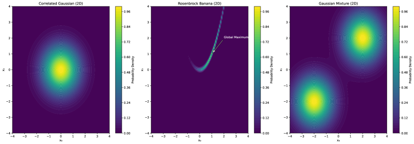
Figure 1: The surface plots corresponding to the three test problems. The global maximum that the sampler needs to find is marked in the case of the Rosenbrock distribution, the two others correspond to a single and double Gaussians respectively.

Correlated Gaussian The simplest test case involves a multivariate Gaussian distribution:

$$\log\mathcal{L}(\mathbf{x})=-\frac{1}{2}\sum_{i=1}^{d}x_{i}^{2}$$ (7)

This distribution tests basic convergence properties and scaling with dimensionality. It establishes a baseline efficiency under ideal conditions, particularly relevant for cosmological applications where approximate Gaussianity often holds near the maximum likelihood.

Rosenbrock (Banana) Distribution The Rosenbrock function, also known as the banana distribution due to its characteristic shape, presents a challenging curved degeneracy:

$$\log\mathcal{L}(\mathbf{x})=-\sum_{i=1}^{d-1}\left[100(x_{i+1}-x_{i}^{2})^{2}+(1-x_{i})^{2}\right]$$ (8)

This distribution tests samplers’ ability to navigate narrow, curved valleys in parameter space, a feature often encountered in cosmological parameter estimation where parameters exhibit strong non-linear correlations. A cosmological example of such curved distribution might come from the degeneracy between the mass density and the Hubble constant Abdalla et al. (2022).

Gaussian Mixture A bimodal distribution testing mode-finding and mixing capabilities:

$$\log\mathcal{L}(\mathbf{x})=\log\left[\exp\left(-\frac{1}{2}\sum_{i=1}^{d}(x_{i}+2)^{2}\right)+\exp\left(-\frac{1}{2}\sum_{i=1}^{d}(x_{i}-2)^{2}\right)\right]$$ (9)

This distribution challenges samplers to properly sample from multiple distinct modes, a situation that arises in various cosmological contexts, like gravitational lensing, neutrino mass hierarchy and modified gravity theories.

4.1 Performance Metrics and Accuracy

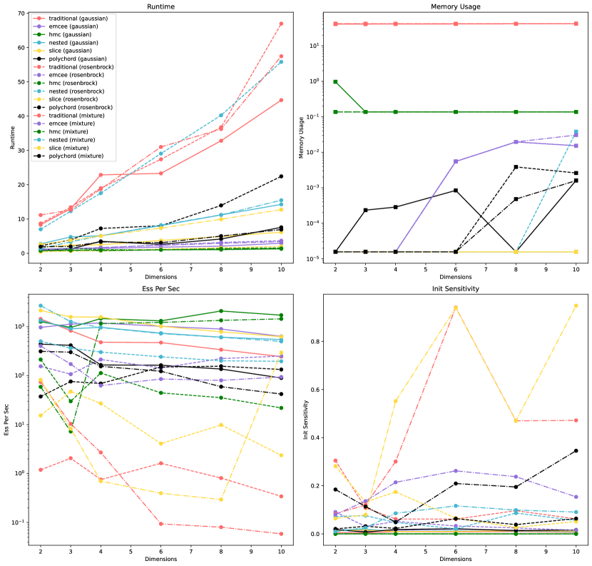
Figure 2: The summary of the metrics we track for the different samplers. We show here the runtime, the memory usage, the ess per sec and the Init Sensitivity.

We focus our analysis on four key metrics: Runtime and Memory usage: measures directly computational cost and memory allocation; Effective Sample Size (ESS) per second: measuring sampling efficiency by calculating how many effectively independent samples are generated per unit time, accounting for autocorrelation in the chains, Init sensitivity: measures the sensitivity to random initialization fluctuation (i.e. starting the code with different seeds) .

To evaluate the accuracy, we use two complementary accuracy metrics, mean-based and distribution-based, evaluating both the ability to find the correct parameter values and to properly explore the target distribution (see the Appendix for details). All metrics are normalized within each test problem to facilitate comparison across different distributions and dimensions.

4.2 Results

The results are shown in Fig. 2 and Fig.3. All samplers perform well on the simple Gaussian case, with HMC and slice showing particularly strong performance. The mean-based and distribution-based metrics align closely, as expected for a unimodal, symmetric distribution. Runtime scaling with dimension for most samplers is modest, with slice sampling, HMC, ensted and emcee showing practically the same efficiency in terms of ESS per second.

The Rosenbrock function reveals significant differences between samplers. Its curved ”banana” shape poses challenges for traditional MCMC and slice methods, evidenced by their declining ESS per second with increasing dimensions. While most samplers maintain reasonable mean accuracy, the distribution-based metric shows larger discrepancies, indicating difficulty in properly exploring the curved parameter space. Here slice and emcee fair worst in terms of accuracy, while the ESS per sec show poor performance for traditional MCMC, slice and HMC.

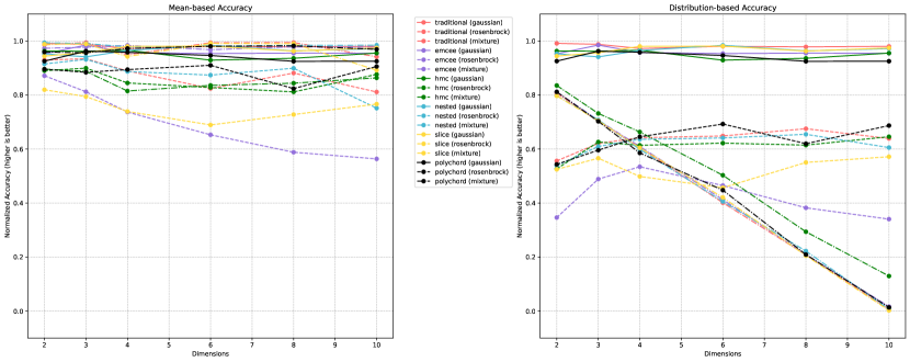
Figure 3: Comparison between the mean accuracy and the distribution accuracy for different samplers. The normalization is described in the Appendix.

The bimodal distribution presents the most challenging test case, with substantial variations in sampler performance. The mean-based accuracy becomes less meaningful here, as the true mean lies between modes. The distribution-based accuracy reveals significant degradation with the increase of dimensions, due to increase probability for the sampler to jump between modes. Here HMC shows a bit better performance in terms of accuracy and ESS per sec on a very slight cost in terms of runtime but requiring more memory.

It is important to note that some metrics require careful interpretation: the ESS measurements, designed for MCMC methods, do not fully capture nested sampling efficiency, better characterized by the ratio of live to dead points at each likelihood threshold. For example, for simple Gaussian distributions, PolyChord maintains reliable accuracy but with lower ESS per second compared to traditional MCMC methods. In the Rosenbrock case, its performance remains stable across dimensions, effectively navigating the curved parameter space due to its slice sampling component. On the other hand, the traditional method was convergent only for the Gaussian distribution. We tried increasing the sample size and the tuning, but that only led to the increase of runtime and memory, not better convergence.

The Init Sensitivity metric is the final metric we track. It tracks the samplers reliability across different random seeds – a key consideration for reproducible cosmological analyses. While most samplers show minimal sensitivity at low dimensions ($<0.005$ for 1D and 2D), we see increasing variability in higher dimensions. This effect becomes more pronounced with the decrease of the accuracy, for example for the Mixture problem. HMC demonstrates notably stable performance across dimensions, likely due to its geometric properties, while traditional MCMC shows moderate increase in sensitivity with dimensionality.

5 Cosmological applications

5.1 Marginalized BAO likelihood

The code uses the marginalized likelihood that uses data from Baryonic acoustic oscillations (BAO), in this case, the newest DESI results Adame et al. (2024), for which the dependence on the Hubble constant ($H_{0}$) and the sound horizon ($r_{d}$) are integrated out. The details on this method can be found in Staicova and Benisty (2022); Benisty et al. (2024) and we’ll leave them out for brevity. The marginalized BAO likelihood provides a good test case due to the fact it has been tested already on more extensive numerical datasets and it also exhibits some of the features of cosmological inference problems – for example the marginalization process might introduce non-Gaussianity, while the dark energy parameters might have curved degeneracies.

The final likelihood depends only on the matter density $\Omega_{m}$, the curvature density $\Omega_{K}$ and the dark energy parameters $w,w_{a}$, where $w$ corresponds to the equation of state. We implemented the six samplers discussed above to the cosmological likelihood and tested each of them on the BAO likelihood with increasing dimensionality (1-4 dimensions), corresponding to different cosmological models: $\Lambda$CDM (1D) with $\Omega_{m}$ as a free parameter, $\Omega_{K}$CDM which adds spatial curvature $\Omega_{K}$ (2D), dark energy model $wwa$CDM (3D) for which the free parameters are $\Omega_{m},w,w_{a}$ and $\Omega_{K}wwa$CDM (4D) which combines all the for parameters. In the study below, we use the following priors: $\Omega_{m}\in(0.1,0.5),\Omega_{K}\in(-0.3,0.3),w\in(-2,0),w_{a}\in(-2,2)$ applied to the respective models.

5.2 Performance Analysis

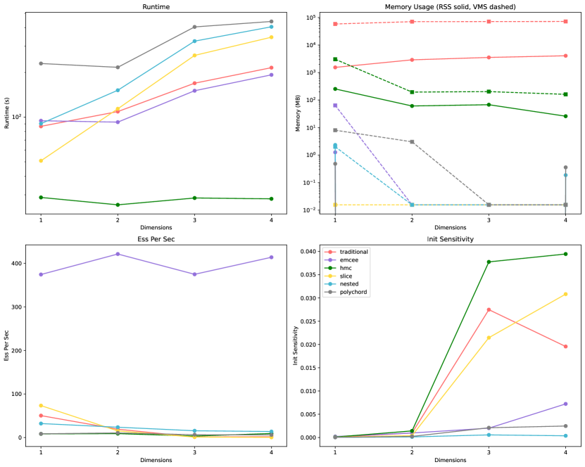
Figure 4: The summary of the benchmark on cosmological models using the different samplers.

Runtime scaling follows approximate power laws with dimension, but coefficients vary substantially between methods. Traditional MCMC, emcee and HMC demonstrate moderate scaling, with HMC showing better performance due to its gradient-based updates. PolyChord and nested sampling show steeper scaling but maintain reliable exploration of the parameter space. Slice demonstrates very steep scaling. In terms of runtime, HMC does best while polychord does worst.

Memory requirements scale distinctly for each sampler implementation. Traditional MCMC shows significant memory use, while HMC maintains relatively stable memory usage through its computational graph optimization, but at the cost of requiring JAX-compatible likelihood functions. Nested sampling methods present unique memory profiling challenges due to their parallel implementation structure, potentially leading to underestimation in our measurements as the memory allocation occurs across multiple processes.

Sampling efficiency, measured through ESS per second 4), demonstrates strong dependence on both dimensionality and parameter type. HMC maintains consistent efficiency up to 3D before showing some decline in 4D, likely due to the increasing complexity of the parameter space affecting its momentum updates. Traditional MCMC shows stable but lower efficiency, while nested samplers achieve consistent performance despite lower raw sampling rates. Slice sampling shows a notable deterioration in performance with dimensionality.

In this case the Init sensitivity demonstrates more significant scaling with dimensions, likely related again with the increase of errors in the constraints. We see that it is quite low in 1D, but for $d>2$, it quickly increases. Here the nested samplers and emcee show most stable performance.

5.3 Accuracy Analysis

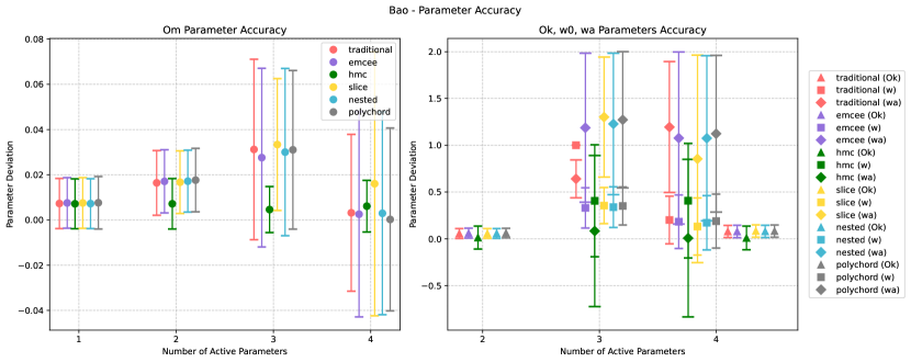
Figure 5: The left panel shows the well constrained $\Omega_{m}$ for all models. The right panel displays deviations for the additional parameters: spatial curvature ($\Omega_{k}$) in the 2D model and the 4D model, equation of state $w$ in the 3D model, and both $w$ and $w_{a}$ in the 4D model.

Parameter constraint quality shown in Fig. 5 varies significantly between cosmological parameters. $\Omega_{m}$ shows consistent accuracy across all samplers and dimensions, with deviations from the fiducial value ($\Omega_{m}=0.3$) typically around $0.007\pm 0.002$. This indicates robust sampling of well-constrained parameters regardless of method choice. We also note that the constraint degrade with the increase of dimensions and also that HMC is particularly good in higher dimensions in terms of accuracy.

The spatial curvature has small deviation from the fiducial value but with big standard deviation $\Omega_{K}=0$ of $0.05\pm 0.05$ with only HMC giving negative mean with higher error ($\Omega_{K}=-0.013\pm 0.12$).

Dark energy parameters prove more challenging, showing significantly larger uncertainties and stronger parameter degeneracies with $w$ constrained much better than $w_{a}$. For the $3D$ case, we see $w=-0.67\pm 0.3$ while the range on $w_{a}$ is much bigger $w_{a}\approx-1\pm 0.8$. Finally, in our test of $OmegA_{K}wwa$CDM we see again big errors, especially in $w_{a}$ but surprisingly tight constraints on $\Omega_{K}$.

The $w-w_{a}$ plane particularly highlights differences between samplers, with nested methods showing advantages in exploring the degenerate parameter space. This pattern reflects the inherent degeneracies in these parameters, the increased difficulty to constrain them as the parameter space expands and the decreased sensitivity of the marginalized likelihood on them.

In conclusion, all samplers maintain comparable performance levels, with no method showing significant advantages in accuracy, though traditional MCMC and emcee exhibit slightly larger uncertainties in the higher-dimensional cases.

5.4 Implementation Challenges

Implementing the benchmark for cosmological likelihood showed few significant challenges. The memory was hard to measure due to the rapid allocation and deallocation of memory and the parallel processing of nested samplers. Furthermore, creating a uniform interface across samplers was a major problem, since it required careful handling of different parameter space representations (unit cube vs. physical space), various input and output formats (for example normal likelihood vs. JAX-compaitble on ) and chain structures and divergent initialization procedures. Consequently, the code required extensive error handling due to numerical instabilities in likelihood evaluations and different convergence behaviors. Finally creating the diagnostics was not trivial. This is because not all samplers provide the same diagnostic metrics (for example we couldn’t not get the acceptance rate for HMC), some diagnostics (like R-hat) require multiple chains and ESS calculations differ between MCMC and nested sampling approaches as seen on the figure.

The results demonstrate that while all methods achieve similar accuracy for well-constrained parameters, their performance diverges significantly for parameters with strong degeneracies. This suggests that method selection for cosmological applications should consider both the specific parameters of interest and computational resource constraints.

6 Discussion and outlook

Bayesian inference in cosmology often requires sampling from complex probability distributions in high-dimensional parameter spaces. The choice of sampling method can significantly impact both the accuracy of results and computational efficiency. Here we examined several of the most basic MCMC methods and tried to benchmark them both in very simple test problems and in realistic cosmological settings. We designed the code using well known Python libraries, facing numerous challenges related to the simultaneous work of all the samplers together. We show that no single method is significantly better than the others and all of them can be used in certain situations.

In particular, traditional MCMC maintains reliable performance but shows limitations in higher dimensions or in complicated distributions. The strong performance of slice sampling in low dimensions suggests simpler methods can still be useful, though one needs to take into account the deterioration of their performance in higher dimensions.

The success of emcee in terms of ESS per second as it combines with increased parameter uncertainties in higher dimensions suggesting that raw sampling efficiency does not necessarily indicate optimal posterior exploration. This observation particularly impacts cosmological applications where accurate uncertainty estimation proves crucial. The nested samplers – nested (dynesty) and PolyChord, on the other hand, while keeping modest ESS per sec demonstrated good accuracy in the accuracy metrics.

To conclude, we would like to discuss some alternatives to simple samplers considered here. Recent years have seen significant advances in sampling methods, particularly those addressing the unique challenges of cosmological applications. These developments broadly fall into several categories, each offering novel approaches to overcome specific limitations of traditional methods.

Neural-based approaches have emerged as a promising direction, with methods like the neural sampling machine (Dutta et al., 2022) utilizing synaptic noise for learning and inference to approximate Bayesian inference. This neural acceleration is particularly relevant for cosmology, where complicated instrumental likelihoods can be computationall expensive. In cases where likelihoods are intractable, likelihood-free inference methods employing neural density estimators (Alsing et al., 2019; Jeffrey et al., 2021) have proven to be powerful alternatives to traditional MCMC approaches.

For multi-modal distributions, common in cosmological applications, several innovative methods have been developed. Parallel tempering (Sambridge, 2014) has shown improved efficiency in exploring such distributions, while Continuous Tempering (Graham and Storkey, 2017) introduces a continuous temperature parameter for smoother transitions between tempered distributions. The challenge of quasi-ergodicity in Monte Carlo simulations has been addressed through various approaches (Neirotti et al., 2000; Frantz et al., 1990), including the use of optimal transport theory for designing more efficient proposal distributions.

Geometric considerations have also driven significant methodological advances. Orbital MCMC (Neklyudov and Welling, 2022) uses principles from Hamiltonian mechanics to preserve geometric structures in the target distribution, while geometric HMC variants (Betancourt and Girolami, 2015; Betancourt, 2018) offer improved adaptation to the target distribution’s geometry through higher-order differential geometric structures. These methods show particular promise for high-dimensional problems with complex geometries, though their practical implementation often requires significant computational resources and expertise.

The integration of machine learning with sampling methods has opened new avenues for improvement. Adaptive Monte Carlo augmented with normalizing flows (Gabrié et al., 2022) combines normalizing flows with MCMC methods, using learned transformations to enhance sampling efficiency. The No-U-Turn Sampler variant of HMC, now standard in frameworks like PyMC and Stan Hoffman et al. (2014) showing how algorithmic improvements can lead to widespread practical adoption.

As cosmological analyses become increasingly sophisticated, understanding the advantages and limitations of these sampling methods becomes crucial. Many of these advanced methods show theoretical promise for next-generation cosmological surveys, where traditional sampling methods may become computationally prohibitive. However, their practical implementation often requires careful consideration of the specific problem context and available computational resources. This complexity underscores the importance of a detailed examination of various sampling approaches to develop more reliable numerical methods for cosmological applications.

Appendix A Accuracy estimates

Mean-based Accuracy For the mean-based accuracy, we compute:

$$\text{Mean Error}=\sqrt{\frac{1}{d}\sum_{i=1}^{d}(\bar{x}_{i}-x_{\text{true},i})^{2}}$$ (10)

where $d$ is the dimension, $\bar{x}_{i}$ is the mean of samples for parameter $i$, and $x_{\text{true},i}$ is the true parameter value. This metric assesses how well samplers recover the true parameters, particularly relevant for point estimation tasks. For weighted samples (as in nested sampling methods), we use the weighted mean $\bar{x}_{i}=\frac{\sum_{j=1}^{N}w_{j}x_{ij}}{\sum_{j=1}^{N}w_{j}}$ where $w_{j}$ are the sample weights.

Distribution-based Accuracy The distribution-based metric varies by test problem to capture the specific features of each distribution:

For the Gaussian case:

$$\text{Gaussian Error}=-\frac{1}{2}\sum_{i=1}^{d}x_{i}^{2}$$ (11)

which directly measures deviation from the zero-centered standard normal distribution.

For the Rosenbrock function:

$$\text{Rosenbrock Error}=\frac{1}{d-1}\sum_{i=1}^{d-1}\left[100(x_{i+1}-x_{i}^{2})^{2}+(1-x_{i})^{2}\right]$$ (12)

which measures how well samples follow the characteristic curved valley of the distribution.

For the Gaussian mixture:

$$\text{Mixture Error}=-\log\left(\exp\left(-\frac{1}{2}\sum_{i=1}^{d}(x_{i}+2)^{2}\right)+\exp\left(-\frac{1}{2}\sum_{i=1}^{d}(x_{i}-2)^{2}\right)\right)$$ (13)

measuring the ability to sample from both modes at $x_{i}=\pm 2$.

The final accuracy scores are normalized using fixed maximum error thresholds: 0.5 for Gaussian, 2.0 for Rosenbrock, and 5.0 for the mixture model.

The mean-based metric is appropriate for unimodal distributions where point estimation is meaningful, while the distribution-based metric better captures performance on multimodal or highly curved distributions where the mean alone may be misleading.

References

- Abdalla et al. [2022] Elcio Abdalla et al. Cosmology intertwined: A review of the particle physics, astrophysics, and cosmology associated with the cosmological tensions and anomalies. JHEAp, 34:49–211, 2022. doi: 10.1016/j.jheap.2022.04.002.
- [2] Carroll C Dong L Fonnesbeck CJ Kochurov M Kumar R Lao J Luhmann CC Martin OA Osthege M Vieira R Wiecki T Zinkov R. Abril-Pla O, Andreani V. Pymc: A modern and comprehensive probabilistic programming framework in python. URL https://github.com/pymc-devs/pymc#citing-pymc.
- Adame et al. [2024] A. G. Adame et al. DESI 2024 VI: Cosmological Constraints from the Measurements of Baryon Acoustic Oscillations. 4 2024.
- Alsing et al. [2019] Justin Alsing, Tom Charnock, Stephen Feeney, and Benjamin Wandelt. Fast likelihood-free cosmology with neural density estimators and active learning. Monthly Notices of the Royal Astronomical Society, 488(3):4440–4458, 2019.
- Benisty et al. [2024] David Benisty, Supriya Pan, Denitsa Staicova, Eleonora Di Valentino, and Rafael C. Nunes. Late-time constraints on interacting dark energy: Analysis independent of H0, rd, and MB. Astron. Astrophys., 688:A156, 2024. doi: 10.1051/0004-6361/202449883.
- Betancourt [2018] Michael Betancourt. A geometric theory of higher-order automatic differentiation. arXiv preprint arXiv:1812.11592, 2018.
- Betancourt and Girolami [2015] Michael Betancourt and Mark Girolami. Hamiltonian monte carlo for hierarchical models. Current trends in Bayesian methodology with applications, 79(30):2–4, 2015.
- Duane et al. [1987] Simon Duane, Anthony D Kennedy, Brian J Pendleton, and Duncan Roweth. Hybrid monte carlo. Physics Letters B, 195(2):216–222, 1987.
- Dutta et al. [2022] Sourav Dutta, Georgios Detorakis, Abhishek Khanna, Benjamin Grisafe, Emre Neftci, and Suman Datta. Neural sampling machine with stochastic synapse allows brain-like learning and inference. Nature Communications, 13(1):2571, 2022.
- Frantz et al. [1990] DD Frantz, David L Freeman, and Jimmie D Doll. Reducing quasi-ergodic behavior in monte carlo simulations by j-walking: Applications to atomic clusters. The Journal of chemical physics, 93(4):2769–2784, 1990.
- Gabrié et al. [2022] Marylou Gabrié, Grant M Rotskoff, and Eric Vanden-Eijnden. Adaptive monte carlo augmented with normalizing flows. Proceedings of the National Academy of Sciences, 119(10):e2109420119, 2022.
- Graham and Storkey [2017] Matthew M Graham and Amos J Storkey. Continuously tempered hamiltonian monte carlo. arXiv preprint arXiv:1704.03338, 2017.
- Handley et al. [2015a] W. J. Handley, M. P. Hobson, and A. N. Lasenby. PolyChord: nested sampling for cosmology. Mon. Not. Roy. Astron. Soc., 450(1):L61–L65, 2015a. doi: 10.1093/mnrasl/slv047.
- Handley et al. [2015b] W. J. Handley, M. P. Hobson, and A. N. Lasenby. polychord: next-generation nested sampling. Mon. Not. Roy. Astron. Soc., 453(4):4385–4399, 2015b. doi: 10.1093/mnras/stv1911.
- Hastings [1970] W Keith Hastings. Monte carlo sampling methods using markov chains and their applications. Biometrika, 57(1):97–109, 1970.
- Hoffman et al. [2014] Matthew D Hoffman, Andrew Gelman, et al. The no-u-turn sampler: adaptively setting path lengths in hamiltonian monte carlo. J. Mach. Learn. Res., 15(1):1593–1623, 2014.
- Jeffrey et al. [2021] Niall Jeffrey, Justin Alsing, and François Lanusse. Likelihood-free inference with neural compression of des sv weak lensing map statistics. Monthly Notices of the Royal Astronomical Society, 501(1):954–969, 2021.
- Koposov et al. [2024] Sergey Koposov, Josh Speagle, Kyle Barbary, Gregory Ashton, Ed Bennett, Johannes Buchner, Carl Scheffler, Ben Cook, Colm Talbot, James Guillochon, Patricio Cubillos, Andrés Asensio Ramos, Matthieu Dartiailh, Ilya, Erik Tollerud, Dustin Lang, Ben Johnson, jtmendel, Edward Higson, Thomas Vandal, Tansu Daylan, Ruth Angus, patelR, Phillip Cargile, Patrick Sheehan, Matt Pitkin, Matthew Kirk, Joel Leja, joezuntz, and Danny Goldstein. joshspeagle/dynesty: v2.1.4, June 2024. URL https://doi.org/10.5281/zenodo.12537467.
- Lewis and Bridle [2002] Antony Lewis and Sarah Bridle. Cosmological parameters from cmb and other data: A monte carlo approach. Physical Review D, 66(10):103511, 2002.
- Metropolis et al. [1953] Nicholas Metropolis, Arianna W Rosenbluth, Marshall N Rosenbluth, Augusta H Teller, and Edward Teller. Equation of state calculations by fast computing machines. The Journal of Chemical Physics, 21(6):1087–1092, 1953.
- Neal [2003] Radford M Neal. Slice sampling. The Annals of Statistics, 31(3):705–767, 2003.
- Neirotti et al. [2000] JP Neirotti, David L Freeman, and JD Doll. Approach to ergodicity in monte carlo simulations. Physical Review E, 62(5):7445, 2000.
- Neklyudov and Welling [2022] Kirill Neklyudov and Max Welling. Orbital mcmc. pages 5790–5814, 2022.
- Phan et al. [2019] Du Phan, Neeraj Pradhan, and Martin Jankowiak. Composable Effects for Flexible and Accelerated Probabilistic Programming in NumPyro. 12 2019.
- Planck Collaboration et al. [2020] Planck Collaboration, N. Aghanim, Y. Akrami, M. Ashdown, et al. Planck 2018 results. vi. cosmological parameters. Astronomy & Astrophysics, 641:A6, 2020.
- Sambridge [2014] Malcolm Sambridge. A parallel tempering algorithm for probabilistic sampling and multimodal optimization. Geophysical Journal International, 196(1):357–374, 2014.
- Skilling [2006] John Skilling. Nested sampling for general bayesian computation. Bayesian Analysis, 1(4):833–859, 2006.
- Speagle [2020] Joshua S. Speagle. dynesty: a dynamic nested sampling package for estimating Bayesian posteriors and evidences. Mon. Not. Roy. Astron. Soc., 493(3):3132–3158, 2020. doi: 10.1093/mnras/staa278.
- Staicova and Benisty [2022] Denitsa Staicova and David Benisty. Constraining the dark energy models using baryon acoustic oscillations: An approach independent of H0 rd. Astron. Astrophys., 668:A135, 2022. doi: 10.1051/0004-6361/202244366.
- Trotta [2008] Roberto Trotta. Bayes in the sky: Bayesian inference and model selection in cosmology. Contemporary Physics, 49(2):71–104, 2008.