Resonance of an object floating within a surface wavefield

Abstract

We examine the interaction between floating cylindrical objects and surface waves in the gravity regime. Given that the impact of resonance phenomena associated with floating bodies, particularly at laboratory scales, remains underexplored, we focus on the influence of the floaters’ resonance frequency on wave emission. We study the response of floating rigid cylinders to external mechanical perturbations. Using an optical reconstruction technique to measure wave fields, we study the natural resonance frequency of the floaters in geometry and their response to incoming waves. The results indicate that the resonance frequency is influenced by the interplay between the cylinder geometry and the solid-to-fluid density ratio. Experiments with incoming waves demonstrate that floaters diffract waves, creating complex patterns of diffusion and retro-diffusion while radiating secondary waves that interfere with the incident wavefield. Minimal wave generation is observed at resonance frequencies. These findings provide insights for elucidating the behavior of larger structures, such as sea ice floes, in natural wave fields.

I INTRODUCTION

Wave-structure interactions [1, 2] are encountered in various engineering applications, such as naval architecture and offshore operations, including ships, platforms, and buoys [3, 4, 5]. Interactions between waves and floating objects also arise in the marginal ice zone (MIZ), the polar region partially covered by ice floes formed of frozen sea ice [6]. The extent of the MIZs is determined by numerous effects, including wave-floes interaction [7, 8, 9], which has been theoretically studied for deformable cylinders [10].

Experimental measurements have also been conducted in wave basin to rationalize wave-floe interactions, and to model the scattering of surface waves by floes [11, 12, 13, 14, 15]. Numerical simulations further extend these efforts [16, 17, 18]. A range of geometries, from floating spheres [19, 20] to complex offshore structures [21, 22, 23, 24], have been investigated. Floating bodies with simple geometry, such as cylindrical objects, exhibit pronounced heaving, pitching, and surging motions when subjected to anisotropic wave fields [25, 26, 27, 28]. However, to the best of our knowledge, there are no quantitative measurements of the wave field generated by a floating object oscillating in an external wave field. In the laboratory-scale experiment we present here, we study the emission of waves by partially immersed cylinders. In particular, we compare the wave field generated by a free oscillating cylinder to the wave field induced by its oscillations when they are triggered by an external wave field. When the frequency of the external wave field is close to the floater’s natural frequency, minimal wave re-emission is observed in the transverse direction.

The manuscript is organized as it follows. In Section II we experimentally characterize the resonance frequency of floating cylindrical bodies and propose a theoretical model for it. In Section III we study the interaction of these bodies with an externally generated wave field, highlighting how the body’s natural frequency affects this interaction. In all cases the system behavior is characterized using an optical technique for the reconstruction of the liquid surface [29, 30].

II NATURAL FREQUENCY OF OSCILLATION OF A FLOATING OBJECT

II.1 Experiments

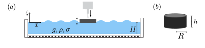
Figure 1: Experimental setup for measuring the natural frequency $f_{0}$ of a floating body. (a) Side-view schematic (not to scale) and (b) body geometry.

We use polyethylene cylinders with density $\rho=0.95\,\rm{g/cm^{3}}$ as floating objects. The cylinder radius $R$ ranges from $R=7.5\,\rm{mm}$ to $30.0\,\rm{mm}$, and the height $h$ ranges from $h=5.0\,\rm{mm}$ to $20.0\,\rm{mm}$ (Fig 1b). The floaters are placed on the surface of water, in a tank with dimensions $78\,\rm{cm}\times 38\,\rm{cm}\times 19\,\rm{cm}$. The water depth of $H=5.0\,\rm{cm}$ ensures that the surface waves are in the deep water regime in the entire range of working frequency. We investigate a wide range of aspect ratios ($h/R$), from $0.17$ to $2.67$. Given the thickness and Young’s modulus of the floaters, they can be considered as rigid bodies in this frequency range. To ensure reproducible wetting conditions and to prevent overwashing, we cover the external surface of each cylinder with adhesive tape.

We first investigate the vertical oscillation mode (heaving) as a function of the floater geometry. Starting from a floater at rest, we perturb its vertical position using a metal rod driven by a shaker. The rod produces a single impact at the floater center. The impact triggers vertical oscillations as sketched in Fig 1a).

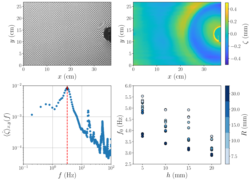
Figure 2: Wave field and resonance frequency of floating cylinders experiencing instantaneous vertical impacts. (a) Top view of a floating cylinder ($R=30\,\rm mm$, $h=15\,\rm mm$) displaced by a rod (as depicted in the setup of Fig. 1a) over a checkerboard pattern with square size $a_{c}=4.0\,\rm mm$. (b) Water surface topography at time $t=1.39\,\rm s$ post impact. (c) Fourier spectrum $|\langle\hat{\zeta}\rangle_{x,y}|(f)$ of the wave field generated by the object perturbation shown in (b), with the resonance frequency $f_{0}=3.16\,\rm Hz$ indicated in red. (d) Measured resonance frequency for floaters with different dimensions. Each data point corresponds to an individual experiment.

To prevent the floater from drifting, we attach loosely the cylinder’s upper edge to the tank walls using two nylon wire, without affecting the vertical motion of the cylinder. The wave topography generated by the floater oscillations is measured using a technique named Fast Checkerboard Demodulation (FCD) [30]. A checkerboard pattern is placed beneath the tank and a camera records at 200 frames per second the surface from above. We then measure the pattern distortion for each video frame and compare it to a static reference image. The distorsion pattern is caused by light refraction at the air-water interface of the checkerboard, and a reconstruction of surface elevation with a sensitivity of $\approx 10\,\mu\text{m}$ (see Fig 2a) can eventually be achieved. Wave propagation predominantly occurred in the deep water regime ($kH\gg 1$, with $k$ the wavenumber). The checkerboard square size $a_{c}=4.0\,\rm{mm}$ is selected to avoid surface reconstruction errors in accordance with the criteria of Moisy et al. [29].

The wavefield is recorded from the instant of impact until the waves reflect back from the tank boundaries. The reconstructed surface $\zeta(x,y,t)$ (see Fig. 2b) is analyzed using Fourier analysis. We first compute $\hat{\zeta}_{x,y}(f)$ the Fourier spectrum in time at all (spatial) locations of the 2D reconstructed wave field. We then average the Fourier spectra in space over the entire reconstructed area. (Fig. 2c) shows the absolute value of $<\hat{\zeta}_{x,y}(f)>$ as a function of frequency $f$ in logarithmic scale. For all our experiments, we observe one large peak with a frequency in the range $2-6$ Hz and a few secondary peaks at much larger frequencies (typically for $f>15$ Hz). To provide an accurate estimate of the frequency of maximum emission $f_{0}$, we fit the peak with a parabolic function to locate precisely the maximum. We also extract the amplitude of the resonance peak from this interpolation. By recording the motion of the floater from the side, we checked that the frequency $f_{0}$ measured from the wave field precisely corresponds to the oscillation frequency of the vertical motion of the cylinder. Figure 2d shows the frequency $f_{0}$ of maximum emission, as a function of the cylinder thickness $h$. The cylinder radius is color-coded. We observe that $f_{0}$ decreases with both the cylinder thickness and the cylinder radius. This indicates that both parameters play a role in the determination of the heaving resonant frequency $f_{0}$.

II.2 Modeling

Historically, floating objects have been studied most notably in Naval contexts, where engineers sought to understand the motion of ships. Complex variables techniques have been exploited to calculate the added mass of two-dimensional hulls atop a fluid of infinite depth as early as 1929 [31]. A more complete investigation of the heaving motion of two-dimensional bodies was performed in later studies [25, 32, 33, 34], that also consider finite-depth effects. The motion of three-dimensional floating bodies has also been investigated in the case of vertical circular cylinders [35] and spheres [36]. The referenced works rely mainly on expansion formulae, and integral expressions, in order to solve for the ensuing motion of floating obstacles. In the present work, we utilise similar theoretical notions to the mentioned papers, but we invoke a simplifying geometric approximation so that an analytical expression for the oscillation frequency observed in our experiments could be attained in terms of physical properties of the disk; the approximation shows excellent agreement with our data (see Fig. 4).

We describe heave oscillations of a buoyant cylinder floating on a free surface of water of density $\rho_{w}$. We denote the cylinder’s submerged height with $h_{s}$. (Fig. 3a). In the limit of high-frequency oscillations, we derive an expression for the added mass and we deduce the natural frequency of oscillation observed in experiments.

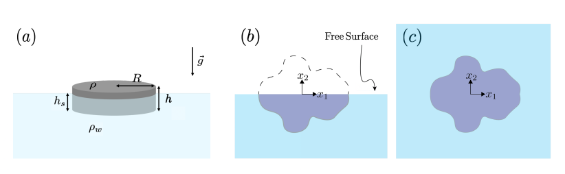
Figure 3: Schematics of a floating cylinder with the variables introduced in the models (a). In the high-frequency limit, the heaving added mass of the shape in panel (b) is equal to half the translatory added mass, $M_{22}$, of the shape in panel (c) in an infinite fluid. The shape in (c) is the union of the submerged portion of the body in (b) and its reflection about the free surface plane.

For a stationary, partially submerged cylinder the equilibrium depth is given by the vertical force balance, $\boldsymbol{F}=0$, where

$$\boldsymbol{F} = \left(-\rho_{w}\pi R^{2}gz-\rho\pi R^{2}hg\right)\hat{\boldsymbol{z}},$$ (1)

$$h_{s} = \frac{\rho}{\rho_{w}}h.$$ (2)

For a small perturbation $\delta z(t)$ of the equilibrium position, a naive force balance on the floating object gives $\rho\pi R^{2}h\ddot{\delta z}=-\rho_{w}\pi R^{2}g\delta z$, which yields the natural frequency of oscillation $\Omega=\sqrt{\rho_{w}g/(\rho h)}$. However, such a calculation overlooks two important considerations. First, the surrounding fluid must be accelerated along with the cylinder, leading to an increase of the effective inertia. Second, the waves at the free surface impose a reaction force on the cylinder.

The High Frequency Limit
The boundary value problem for a heaving cylinder is inherently complex, even when assuming potential flow and linearized boundary conditions. In the following, we use a high-frequency approximation to derive an asymptotic expression for the resonant frequency. We take the limit $\Omega^{2}L/g\rightarrow\infty$, with $L$ the length of the floating body, $g$ the acceleration due to gravity, and $\Omega$ the oscillation frequency. The problem then simplifies as the boundary condition on the free surface reduces to $\phi=0$, where $\phi$ is the velocity potential, while the standard boundary conditions remain applicable elsewhere (see Bai [34] and Ursell [32, §2]). Note that for a typical experiment, with $L=2R$ and $\Omega=2\pi f_{0}$, giving $\Omega^{2}L/g\sim 1-4$. Though these values are not extremely large, we still take the high-frequency limit as the first approximation to our problem.

We use the high frequency limit to compute the added mass, by reflecting the submerged portion of a body and then halving the resultant added mass, referred to as the method of duplicated models [37, p. 135] (see sketch in figure 3(c)). For a vertical translation of the body at some velocity, $\phi(x,y,-z)=-\phi(x,y,z)$ by symmetry, which implies $\phi(x,y,0)=0$. As a consequence, the potential $\phi$ around the shape sketched in figure 3(c) restricted to the domain $z<0$ is a solution to the boundary value problem outlined by Bai [34]. Since the flow magnitude is symmetric about $z=0$, half the energy of the flow around the translating shape in figure 3(c) is in the upper half plane and half is in the lower half-plane. Thus, the added mass for the body in figure 3(b) is precisely half of the added mass for the shape in figure 3(c).

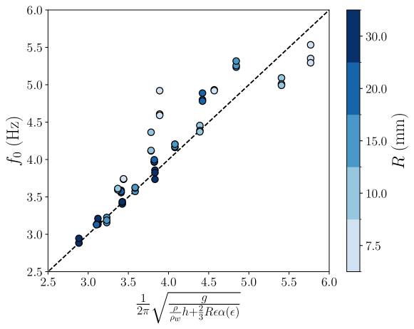
Figure 4: Experimental data compared to our theoretical model, using (5). Each point in the plot represents a single experiment. Cylinder radii are given by color code. For a given radius, cylinder heights are, from right to left in the plot: $h=5\,\rm{mm}$, $h=10\,\rm{mm}$, $h=15\,\rm{mm}$, $h=20\,\rm{mm}$.

Added Mass of Submerged Cylinders: An Ellipsoidal Approximation

To compute the added mass of a floating cylinder of radius $R$ and submerged portion $h_{s}$, we instead compute the added mass of an immersed cylinder of height $2h_{s}$ and then divide by a factor of two, according to the method presented in the previous section. To avoid matching issues at the cylinder corner, we approximate the cylinder by an ellipsoid with semi-axis $h_{s}$ along the vertical direction and radii $R$ along the other two directions. We compute the potential flow around an ellipsoid traveling along its axis at speed $U$ as the solution to a Laplace problem in ellipsoidal coordinates. Next, the kinetic energy of the flow is computed explicitly (see Lamb [38, Eq. 11 of §114]. By considering pure translational motion of the ellipsoid along its semi-axis of radius $h_{s}$, the translational added mass $M_{22}$ writes:

$$M_{22}=\rho_{w}\frac{4\pi h_{s}R^{2}}{3}\frac{\sqrt{1/\epsilon^{2}-1}-\acos{\left(\epsilon\right)}}{\acos{\left(\epsilon\right)-\epsilon\sqrt{1-\epsilon^{2}}}},$$ (3)

where $\epsilon\equiv h_{s}/R$. Considering the additional movement of the surrounding fluid, we perform the force balance now including the effect of the added mass. The equation of motion then becomes,

$$(\rho\pi hR^{2}+M_{22})\ddot{\delta z}+\rho_{w}\pi R^{2}g\delta z=0.$$ (4)

From this equation, we deduce the natural frequency of oscillation of the body,

$$\Omega=\sqrt{\frac{\rho_{w}g\pi R^{2}}{\rho h\pi R^{2}+M_{22}/2}}=\sqrt{\frac{g}{rh+\frac{2R}{3}\epsilon\alpha{\left(\epsilon\right)}}},$$ (5)

where $r=\rho/\rho_{w}$ and

$$\alpha{\left(\epsilon\right)}=\frac{\sqrt{1/\epsilon^{2}-1}-\acos{\left(\epsilon\right)}}{\acos{\left(\epsilon\right)-\epsilon\sqrt{1-\epsilon^{2}}}}.$$ (6)

Note that in this formulation, we have neglected the memory convolution term that becomes important as the wave field builds up [35, see Eq. 31], and thus the frequency is expected to be valid on short time scales or in more situations when the history integral remains small.

We now compare the theoretical prediction with the cylinder resonance frequency $f_{0}$ measured experimentally in Fig 4. Our model is in excellent agreement with the experimental frequency data. The agreement is especially strong for smaller values of the parameter $\Omega$ (parameter on horizontal axis), in agreement with the fact that our approximation is most valid for low frequencies.

III FLOATING OBJECT IN AN EXTERNAL WAVEFIELD

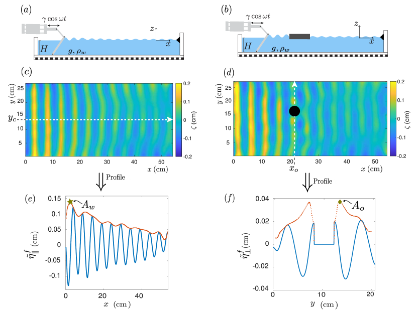
Figure 5: Experimental setups and sample data for characterizing the wave field in the vicinity of a floating object: configuration without (a,c,e) and with (b,d,f) cylindrical floater. (a, b) Schematics of the experimental setups (not to scale), in which a wavemaker generates harmonic waves in the tank. (c, d) Sample instantaneous height fields $\zeta(x,y)$ with wavemaker frequency $f=6.0\,\rm Hz$. In (d) the floating cylinder has radius $R=20\,\rm mm$ and height $h=10\,\rm mm$. (e) Processed spatio-temporal profile along the dashed line at $y=y_{c}$ in (c). (f) Processed spatio-temporal profile along the dashed line at $x=x_{o}$ in (d), passing through the center of the floating object. Blue lines show the wave height at a given time, while red lines are the envelopes of the processed signal.

We now examine the interaction between the floater and externally generated surface waves. The experiment is designed to look at the wave field near the floating cylinder. We compare two configurations: in the first configuration, the floating object can move freely at the surface, in response to the incoming wave field (see Fig. 5b); in the second configuration, the floater is attached to the bottom of the water tank with a rigid stick (Fig. 7a). We generate the surface wave using a moving plate connected to a linear motor, as sketched in Fig 5. A wave absorber, made of triangular shapes of expanded polystyrene, is placed at the end edge to reduce wave reflection. The wave field is recorded at 100 frames per second during 10 seconds. The wave field $\zeta(x,y,t)$ is measured with the surface reconstruction technique described in Section I [30].

In the free-floating configuration, a cylinder is placed 10 cm away from the plate far from the lateral edges. We systematically vary the wave frequency $f$ while maintaining a constant plate displacement amplitude. Figs. 5c and 5d show the comparison between the wave field with and without the object. In the presence of the object, we observe the superposition of the incoming wave, the reflected waves, and the waves emitted by the oscillations of the cylinder. We focus on wave emission near the natural frequency $f_{0}$ of the floater.

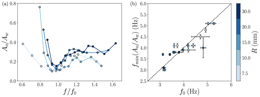
Figure 6: Effect of the object on the incoming wave field. (a) Normalized amplitude $A_{o}/A_{w}$ of the waves emitted in a direction orthogonal to the incoming wave vector as a function of the normalized frequency of the incoming waves, $f/f_{0}$, for various radii $R$ and fixed height $h=10\>\rm mm$. (b) Comparison between the frequency at which the normalized amplitude is minimal, $f_{\rm min}(A_{o}/A_{w})$, and the natural frequency $f_{0}$ of the cylinders for all the tested geometries.

First, we extract from the wave field a one-dimensional spatiotemporal profile in the absence of the floater, ${\eta}_{\parallel}(x,t)=\zeta(x,y=y_{c},t)$, parallel to the generated wave vector, where $y=y_{c}$ is the tank centerline (Fig.5c). After filtering in time and space we obtain $\tilde{\eta}_{\parallel}^{f}(x,t)$ (refer to supplementary material, section II A, for details on signal processing). Computing the enveloppe of $\tilde{\eta}_{\parallel}^{f}(x,t)$ yields to the maximum wave amplitude $A_{w}(\tilde{\eta}_{\parallel}^{f})$, at each frequency (see Fig. 5e). This serves as a reference for later comparisons with the wave field in the presence of the object. We proceed by analysing the interaction between the incoming wave field and the free-floating cylinder. We extract spatio-temporal profiles ${\eta}_{\perp}(y,t)=\zeta(x=x_{o},y,t)$, perpendicular to the generated wave vector, where $x=x_{o}$ is the coordinate of the object’s center of mass (Fig.5d). After filtering we obtain $\tilde{\eta}_{\perp}^{f}(y,t)$, which represents only the waves re-emitted by the object in response to the incoming wave field, as isolated through the filtering process (refer to supplementary material, section II B, for details on signal processing). From this filtered signal, we extract the maximum wave amplitude $A_{o}(\tilde{\eta}_{\perp}^{f})$ (Fig. 5f).

The ratio of re-emitted to undisturbed wave amplitudes, $A_{o}/A_{w}$, is used to quantify the object’s influence on the incoming wave field. The ratio $A_{o}/A_{w}$ is measured for multiple object geometries varying both the radius $R$ and the height $h$ of the cylinder. Fig. 6a shows the amplitude ratio as a function of the excitation frequency $f/f_{0}$. We observe that the wave emission in the transverse direction is minimal close to the floater’s resonance frequency $f_{0}$. This behavior suggests that the object absorbs the wave energy at its natural frequency, resulting in a decrease of the wave emission in the transverse direction. A similar trend is observed for a fixed height (see supplementary material, section III). For each floater, we extract the frequency $f_{\rm min}$ corresponding to the minimum of emission in the transverse direction. Figure 6b shows $f_{\rm min}$ as a function of the natural frequency $f_{0}$ of the floater. We observe that $f_{0}$ is a proxy for $f_{\rm min}$ for all the geometries considered.

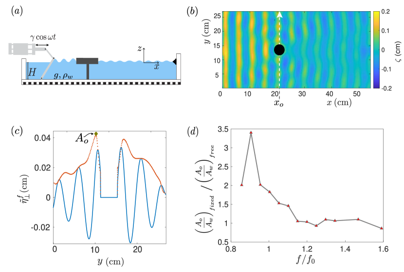
Figure 7: Experimental setup and sample data for characterizing the wave field in the vicinity of a fixed object. (a) Schematic of the experimental setup (not to scale). The floater is attached to the water tank via a metal stick. (b) Snapshot of the reconstructed wave field with forcing frequency $f=6.0\,\rm Hz$. The floater has radius $R=20\,\rm mm$ and height $h=10\,\rm mm$. (c) A filtered spatio-temporal profile along the dashed line at $x=x_{o}$ in (b), passing through the center of the object. The blue line shows the wave height at a given time, while the red line is the envelope of the processed signal. The maximum of the envelope is noted $A_{o}$. (d) Ratio of the normalized amplitudes of wave emitted in the transverse direction by the fixed and the free object as a function of the normalized forcing frequency $f/f_{0}$.

To further highlight the effect of the object motion on the wave emission, we conducted experiment in the second configuration, with a cylinder fixed to the bottom of the tank (Fig. 7a,b,c). The cylinder has the same geometry than the free-floating cylinders. The ratios $A_{o}/A_{w}$ of both free and fixed cylinder are compared in Fig. 7d. Near resonance, the fixed object exhibited greater transversal wave emission compared to the free-floating object. For an excitation frequency higher than $1.2f_{0}$, the two configurations show a similar response. These observations support the hypothesis that at resonance the free floater absorbs and redistributes wave energy unevenly. The floater radiates energy, leading to complex interactions between the emitted and diffracted wave fields, which may explain the reduced emission efficiency. In contrast, the fixed object, unable to oscillate, only reflects and diffracts the incoming waves.

IV CONCLUSION

We have investigated the interaction of a floating cylinder with surface waves in laboratory-scale experiments. In the first part, the bodies’ natural frequencies of oscillation were experimentally characterized and theoretically rationalized in the absence of external wave fields. We show that the resonance frequency of the heaving motion corresponds to the maximum of wave emission. The resonance frequency $f_{0}$ depends on the cylinder radius $R$ and its thickness $h$. We present a theoretical model that rationalizes the observed resonance frequencies for all the body dimensions characterized experimentally. We show that, in the high-frequency limit, the added mass of a floating body corresponds to half the added mass of the same body when it is fully submerged in the fluid bulk. Although this hypothesis is not fulfilled for heaving motions, the comparison with the experimental resonant frequency is quantitative. In the second part, we studied the effects of the floater vertical motion on the re-emitted wave field. We measure the wave field re-emitted by the floating cylinder and we show that, in the transverse direction, the re-emitted wave exhibits a minimum of emission for excitation frequency close to the body resonance frequency $f_{0}$. By comparing the wave fields re-emitted by a fixed and a free-floating cylinder with same dimension, we proved that the body oscillations are indeed responsible for the observed minimal transverse emission.

SUPPLEMENTAL MATERIAL

I. The Disk Limit: An Uniform Approximation

To study the case of a thin floating disk, we can take the limit $\epsilon\rightarrow 0$. In the expression of the resonance frequency of the main text, we see that the product $\epsilon\alpha(\epsilon)$ tends to $2/\pi$. Thus, for small values of $\epsilon$, the frequency reduces to

$$\Omega(\epsilon\rightarrow 0)\rightarrow\sqrt{\frac{g}{rh+\frac{4R}{3\pi}}}.$$ (7)

Naively using this formula over the whole range of experiments, even though in many cases $\epsilon=\mathcal{O}\left(1\right)$, we find a good agreement with the experiment, as depicted in figure 8.

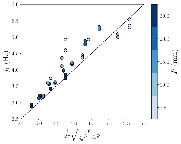
Figure 8: Experimental data compared to our theoretical model, using the approximated formula (7). Each point in the plot represents a single experiment. Cylinder radii are depicted using a color code. For a given radius, cylinder heights are, from right to left in the plot : $h=5\,\rm{mm}$, $h=10\,\rm{mm}$, $h=15\,\rm{mm}$, $h=20\,\rm{mm}$.

One might then ask the question: for arbitrary $\rho,\rho_{w},R,h$, how well does $\Omega(\epsilon=0)$ do at approximating the natural frequency more generally when $\epsilon\neq 0$? To answer this question, we examine the ratio $\Omega(\epsilon=0)/\Omega(\epsilon)$. When this ratio is equal to unity, the approximation is exact. We compute.

$$\frac{\Omega(\epsilon=0)}{\Omega(\epsilon)}=\sqrt{\frac{rh+\frac{2R}{3}\epsilon\alpha\left(\epsilon\right)}{rh+\frac{4R}{3\pi}}}=\sqrt{\frac{1+\frac{2}{3}\alpha\left(\epsilon\right)}{1+\frac{4}{3\pi\epsilon}}},$$ (8)

which only depends on $\epsilon$. Furthermore, by plotting this ratio as a function of epsilon, we see that

$$0.96<\Omega(\epsilon=0)/\Omega(\epsilon)<1$$

for all values of $\epsilon$. Remarkably, one may invoke the approximation outlined in (7) for any density ratio $r$, radius $R$, and height $h_{0}$, and be guaranteed that the error, as compared to the true solution of equation (5), is less than about 4%. Thus, equation (7) represents a very valuable approximation for estimating the natural vibration of a floating cylinder.

II. Signal processing for profile extraction

II A. Parallel profile

The spatio-temporal profile reported in section III of the main text is processed in the Fourier space [39] to filter the waves reflected by the boundaries of the tank, and to mitigate spurious fluctuations associated with low wave numbers. This Fourier filtering process involved: transforming the profiles $\eta_{\parallel}(x,t)$ into the spatial and temporal frequencies domain using the Fourier transform $\mathcal{F}$; applying a filter function $H(k,\omega)$ to suppress undesired frequencies; transforming the filtered profiles back to the spatio-temporal domain using the inverse Fourier transform $\mathcal{F}^{-1}$. These steps can be written as:

$$\hat{\eta}_{\parallel}(k,\omega)=\mathcal{F}[\eta_{\parallel}(x,t)],$$

$$\tilde{\eta}_{\parallel}(x,t)=\mathcal{F}^{-1}[H(k,\omega)\hat{\eta}_{\parallel}(k,\omega)],$$

Where, $\hat{\eta}_{\parallel}(k,\omega)$ corresponds to the Fourier transformation of the horizontal profile and, $\tilde{\eta}_{\parallel}(x,t)$ represents the filtered spatio-temporal signal. This filtered signal is then demodulated at the excitation frequency $f$, leading to a function $\tilde{\eta}_{\parallel}^{f}(x,t)$. A frame of this demodulated profile is represented as the blue curve in figure 5e in the main text. In order to measure the incoming wave amplitude, we extract the envelope of this demodulated profile via a peak detection algorithm that detects the local maxima of the demodulated curve $\tilde{\eta}_{\parallel}^{f}(x,t)$ for all time steps. The envelope curve $E_{\parallel}(\tilde{\eta}_{\parallel}^{f})$ is represented in red in figure 5e in the main text.

II B. Perpendicular profile

First, a filter $H_{r}(k,\omega)$ is applied to the transverse profile in the Fourier space to filter the waves reflected by the boundaries of the tank. Then, Butter-worth filter function $H_{bw}(k,\omega)$ is applied to suppress undesired frequencies at low and high wave numbers [40, 41]. This filtered signal is then transformed back to a spatiotemporal signal $\tilde{\eta}_{\perp}(y,t)$ using inverse Fourier transform $\mathcal{F}^{-1}$ :

$$\hat{\eta}_{\perp}(k,\omega)=\mathcal{F}[\eta_{\perp}(y,t)],$$

$$\tilde{\eta}_{\perp}(y,t)=\mathcal{F}^{-1}[H_{r}(k,\omega)H_{bw}(k,\omega)\hat{\eta}_{\perp}(k,\omega)].$$

Finally, the profile $\tilde{\eta}_{\perp}(y,t)$ is demodulated at the excitation frequency $f$ to get the spatio-temporal signal $\tilde{\eta}_{\perp}^{f}(y,t)$, plotted as the blue curve in figure 5f in the main text. The maximum amplitude of the waves emitted by the object in this direction, is obtained by extracting the envelope of $\tilde{\eta}_{\perp}^{f}(y,t)$, as described in the previous section. The envelope $E_{\perp}(\tilde{\eta}_{\perp}^{f})$ is represented in red in figure 5f in the main text.

III. Propagation waves of the cylinders for a fixed height

Using the same approach as in Figure 6 a of the main text, the ratio $A_{o}/A_{w}$ was determined for different heights of the free-floating cylinders with fixed radius $R=15\>\rm mm$. The results are plotted in Figure 9 as a function of the excitation frequency $f$ normalized by the measured resonance frequency $f_{0}$ of each body. Here also the system exhibits a minimum value of the ratio $A_{o}/A_{w}$ at an excitation frequency close to the resonance frequencie. Therefore, near its resonance frequency $f_{0}$, a cylindrical object shows a reduced emission efficiency in the direction orthogonal to the initial wave propagation.

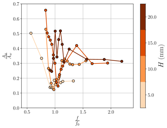
Figure 9: Normalized amplitude $A_{o}/A_{w}$ of the waves emitted in a direction orthogonal to the incoming wave vector as a function of the normalized frequency of the incoming waves, $f/f_{0}$, for various heights $h$ and fixed radius $R=15\>\rm mm$.