A new rotation-free isogeometric thin shell formulation and a corresponding continuity constraint for patch boundaries

This is a corrected version of the published journal article.  All corrections are mark-

ed in green. They were typographical errors that did not affect simulation results.

Abstract: This paper presents a general non-linear computational formulation for rotation-free thin shells based on isogeometric finite elements. It is a displacement-based formulation that admits general material models. The formulation allows for a wide range of constitutive laws, including both shell models that are extracted from existing 3D continua using numerical integration and those that are directly formulated in 2D manifold form, like the Koiter, Canham and Helfrich models. Further, a unified approach to enforce the $G^{1}$-continuity between patches, fix the angle between surface folds, enforce symmetry conditions and prescribe rotational Dirichlet boundary conditions, is presented using penalty and Lagrange multiplier methods. The formulation is fully described in the natural curvilinear coordinate system of the finite element description, which facilitates an efficient computational implementation. It contains existing isogeometric thin shell formulations as special cases. Several classical numerical benchmark examples are considered to demonstrate the robustness and accuracy of the proposed formulation. The presented constitutive models, in particular the simple mixed Koiter model that does not require any thickness integration, show excellent performance, even for large deformations.

Keywords: Nonlinear shell theory, Kirchhoff–Love shells, rotation–free shells, Isogeometric analysis, $C^{1}$-continuity, nonlinear finite element methods

List of important symbols

$\mathbf{1}$	identity tensor in $\mathbb{R}^{3}$
$a$	determinant of matrix $[a_{\alpha\beta}]$
$A$	determinant of matrix $[A_{\alpha\beta}]$
$\boldsymbol{a}_{\alpha}$	co-variant tangent vectors of surface $\mathcal{S}$ at point $\boldsymbol{x}$; $\alpha=1,2$
$\boldsymbol{A}_{\alpha}$	co-variant tangent vectors of surface $\mathcal{S}_{0}$ at point $\boldsymbol{X}$; $\alpha=1,2$
$\boldsymbol{a}_{\alpha,\beta}$	parametric derivative of $\boldsymbol{a}_{\alpha}$ w.r.t. $\xi^{\beta}$
$\boldsymbol{a}_{\alpha;\beta}$	co-variant derivative of $\boldsymbol{a}_{\alpha}$ w.r.t. $\xi^{\beta}$
$a_{\alpha\beta}$	co-variant metric tensor components of surface $\mathcal{S}$ at point $\boldsymbol{x}$
$A_{\alpha\beta}$	co-variant metric tensor components of surface $\mathcal{S}_{0}$ at point $\boldsymbol{X}$
$a^{\alpha\beta\gamma\delta}$	contra-variant components of the derivative of $a^{\alpha\beta}$ w.r.t. $a_{\gamma\delta}$
$b$	determinant of matrix $[b_{\alpha\beta}]$
$B$	determinant of matrix $[B_{\alpha\beta}]$
$\boldsymbol{b}$	curvature tensor of surface $\mathcal{S}$ at point $\boldsymbol{x}$
$\boldsymbol{b}_{\mathrm{0}}$	curvature tensor of surface $\mathcal{S}_{0}$ at point $\boldsymbol{X}$
$\boldsymbol{B}$	left Cauchy-Green tensor of the shell mid-surface
$b_{\alpha\beta}$	co-variant curvature tensor components of surface $\mathcal{S}$ at point $\boldsymbol{x}$
$B_{\alpha\beta}$	co-variant curvature tensor components of surface $\mathcal{S}_{0}$ at point $\boldsymbol{X}$
$\tilde{b}^{\alpha\beta}$	contra-variant components of the adjugate tensor of $b_{\alpha\beta}$
$\mathbf{B}$	matrix of the coefficients of the Bernstein polynomials for element $\Omega^{e}$
$c$	bending stiffness
$c^{\alpha\beta\gamma\delta}$	contra-variant components of the derivative of $\tau^{\alpha\beta}$ w.r.t. $a_{\gamma\delta}$
$\boldsymbol{C}$	right Cauchy-Green tensor of the shell mid-surface
$\tilde{\boldsymbol{C}}$	right Cauchy-Green tensor of a 3D continuum
$\boldsymbol{C}^{*}$	right Cauchy-Green tensor of a shell layer
$\mathbf{C}^{e}$	Bézier extraction operator for finite element $\Omega^{e}$
$\boldsymbol{d}$	shell director vector
$d^{\alpha\beta\gamma\delta}$	contra-variant components of the derivative of $\tau^{\alpha\beta}$ w.r.t. $b_{\gamma\delta}$
$\delta...$	variation of $...$
$\epsilon$	penalty parameter
$\boldsymbol{E}$	Green-Lagrange strain tensor of the shell mid-surface
$e^{\alpha\beta\gamma\delta}$	contra-variant components of the derivative of $M_{0}^{\alpha\beta}$ w.r.t. $a_{\gamma\delta}$
$\boldsymbol{f}$	prescribed surface loads
$f^{\alpha}$	in-plane components of $\boldsymbol{f}$
$f^{\alpha\beta\gamma\delta}$	contra-variant components of the derivative of $M_{0}^{\alpha\beta}$ w.r.t. $b_{\gamma\delta}$
$\mathbf{f}^{e}_{\bullet}$	discretized finite element force vector
$\boldsymbol{F}$	deformation gradient of the shell mid-surface
$\tilde{\boldsymbol{F}}$	deformation gradient of a 3D continuum
$g$	determinant of matrix $[g_{\alpha\beta}]$
$G$	determinant of matrix $[G_{\alpha\beta}]$
$\boldsymbol{g}_{\alpha}$, $\boldsymbol{g}_{3}$	current tangent and normal vectors of a shell layer; $\alpha=1,2$
$\boldsymbol{G}_{\alpha}$, $\boldsymbol{G}_{3}$	reference tangent vectors and normal of a shell layer; $\alpha=1,2$
$g_{\mathrm{c}}$	$G^{1}$-continuity and symmetry constraints
$g_{\alpha\beta}$	co-variant components of the metric tensor of $\mathcal{S}^{*}$
$G_{\alpha\beta}$	co-variant components of the metric tensor of $\mathcal{S}_{0}^{*}$
$G_{\mathrm{ext}}$	external virtual work
$G_{\mathrm{int}}$	internal virtual work
$\Gamma^{\gamma}_{\alpha\beta}$	Christoffel symbols of the second kind
$H$	mean curvature of surface $\mathcal{S}$ at $\boldsymbol{x}$
$H_{0}$	mean curvature of surface $\mathcal{S}_{0}$ at $\boldsymbol{X}$
$\boldsymbol{i}$	identity tensor in $\mathcal{S}$
$\boldsymbol{I}$	identity tensor in $\mathcal{S}_{0}$
$I_{1}$	first invariant of $\boldsymbol{C}$
$\tilde{I}_{1}$	first invariant of $\tilde{\boldsymbol{C}}$
$J$	surface area change
$\tilde{J}$	volume change of a 3D continuum
$J_{a}$	Jacobian of the mapping $\mathcal{P}\rightarrow\mathcal{S}$
$J_{A}$	Jacobian of the mapping $\mathcal{P}\rightarrow\mathcal{S}_{0}$
$\mathbf{k}^{e}_{\bullet}$	finite element tangent matrices
$\kappa$	Gaussian curvature of surface $\mathcal{S}$ at $\boldsymbol{x}$
$\boldsymbol{\kappa}$	pull-back of the curvature tensor $\boldsymbol{b}$
$\boldsymbol{K}$	relative curvature tensor
$K$	surface bulk modulus
$\tilde{K}$	bulk modulus of 3D continua
$\mathcal{L}$	patch boundary on which edge rotation conditions are prescribed
$\lambda_{i}$	principal stretches of surface $\mathcal{S}$ at $\boldsymbol{x}$
$\mu$	surface shear modulus
$\tilde{\mu}$	shear modulus of 3D continua
$\boldsymbol{\mu}_{0}$	moment tensor in the reference configuration
${\boldsymbol{\mu}}$	moment tensor in the current configuration
$M^{\alpha\beta}$, $M_{0}^{\alpha\beta}$	contra-variant bending moment components
$\boldsymbol{n}$, $\tilde{\boldsymbol{n}}$	surface normals of $\mathcal{S}$ at $\boldsymbol{x}$
$\boldsymbol{N}$, $\tilde{\boldsymbol{N}}$	surface normals of $\mathcal{S}_{0}$ at $\boldsymbol{X}$
$\mathbf{N}$	array of NURBS-based shape functions
$\hat{\mathbf{N}}^{e}$	array of B-spline basis functions in terms of the Bernstein polynomials
$\hat{N}^{e}_{A}$	B-spline basis function of the $A^{\mathrm{th}}$ control point; $A=1,~...,~n$
$N^{\alpha\beta}$	total, contra-variant components of $\sigma$
$\nu$	unit normal on $\partial\mathcal{S}$
$\xi$	out-of-plane coordinate
$\xi^{\alpha}$	in-plane coordinates; $\alpha=1,2$
$p$	external pressure
$\mathcal{P}$	parametric domain spanned by $\xi^{1}$ and $\xi^{2}$
$P$	shell material point
$\Pi_{\mathcal{L}}$	potential of the constraint used to enforce edge rotation conditions
$\varphi$	deformation map of surface $\mathcal{S}$
$q$	Lagrange multiplier for the continuity constraint
$\rho$	areal density of surface $\mathcal{S}$
$\mathcal{S}$	current configuration of the shell surface
$\mathcal{S}_{0}$	reference configuration of the shell surface
$\mathcal{S}^{*}$	current configuration of a shell layer
$\mathcal{S}_{0}^{*}$	reference configuration of a shell layer
$\partial\mathcal{S}$	boundary of $\mathcal{S}$
$\boldsymbol{S}$	second Piola-Kirchhoff stress tensor of the shell
$\tilde{\boldsymbol{S}}$	second Piola-Kirchhoff stress tensor of a 3D continuum
$S^{\alpha}$	contra-variant, out-of-plane shear stress components
$\sigma$	Cauchy stress tensor of the shell
$\tilde{}\mbox{\boldmath$\sigma$}$	Cauchy stress tensor of a 3D continuum
$\sigma^{\alpha\beta}$	stretch related, contra-variant components of $\sigma$
$t$	current shell thickness
$T$	reference shell thickness
$\boldsymbol{T}$	traction acting on a cut $\partial\mathcal{S}$ normal to $\nu$
$\boldsymbol{T}^{\alpha}$	traction acting on a cut $\partial\mathcal{S}$ normal to $\boldsymbol{a}^{\alpha}$
$\tau$	unit direction along a surface boundary
$\tilde{}\mbox{\boldmath$\tau$}$	Kirchhoff stress tensor of a 3D continuum
$\tau^{\alpha\beta}$	contra-variant components of the Kirchhoff stress tensor of the shell
$\tilde{\tau}^{\alpha\beta}$	in-plane components of $\tilde{}\mbox{\boldmath$\tau$}$
$\boldsymbol{v}$	velocity, i.e. the material time derivative of $\boldsymbol{x}$
$\mathcal{V}$	space for admissible variations $\delta\boldsymbol{x}$
$w_{A}$	NURBS weight of the $A^{\mathrm{th}}$ control point ($\hat{=}$ FE node); $A=1,~...,~n$
$W$	strain energy density function per reference area
$\tilde{W}$	strain energy density function per reference volume
$\boldsymbol{x}$	current position of a surface point on $\mathcal{S}$
$\boldsymbol{X}$	initial position of $\boldsymbol{x}$ on the reference surface $\mathcal{S}_{0}$
$\tilde{\boldsymbol{x}}$	current position of a material point of a 3D continuum
$\tilde{\boldsymbol{X}}$	reference position of a material point of a 3D continuum
$\mathbf{x}_{e}$	array of all nodal positions for finite element $\Omega^{e}$
$\mathbf{X}_{e}$	array of all nodal positions for finite element $\Omega^{e}_{0}$
$\Omega^{e}$	current configuration of finite element $e$
$\Omega^{e}_{0}$	reference configuration of finite element $e$

1 Introduction

This work presents a new rotation-free isogeometric finite element formulation for general shell structures. The focus here is on solids, even though the formulation generally also applies to liquid shells. The formulation is based on Sauer and Duong, (2015), who provide a theoretical framework for Kirchhoff–Love shells under large deformations and nonlinear material behavior suitable for both solid and liquid shells.

From the computational point of view, among the existing shell theories, the rotation-free Kirchhoff–Love shell theory is attractive since it only requires displacement degrees of freedom in order to describe the shell behavior. The necessity of at least $C^{1}$-continuity across shell elements and their boundaries is the main reason why this formulation is not widely used in practical finite element analysis. Although various efforts have been made for imposing $C^{1}$-continuity on Lagrange elements (see e.g. Oñate and Zárate, (2000); Brunet and Sabourin, (2006); Stolarski et al., (2013); Munglani et al., (2015) and references therein), the proposed computational formulations are usually either expensive or difficult to implement. Due to this cost and complexity, finite shell elements derived from Reissner–Mindlin theory, which require only $C^{0}$-continuity but need additional rotational degrees of freedom, are more widely used (Simo and Fox,, 1989; Simo et al.,, 1990; Bischoff and Ramm,, 1997; Yang et al.,, 2000; Bischoff et al.,, 2004; Wriggers,, 2008). It is worth noting that there are some other formulations that are different from the above prevailing approaches, like extended rotation-free shells including transverse shear effects (Zárate and Oñate,, 2012), rotation-free thin shells with subdivision finite elements (Cirak et al.,, 2000; Cirak and Ortiz,, 2001; Green and Turkiyyah,, 2005; Cirak and Long,, 2010), meshfree Kirchhoff–Love shells (Ivannikov et al.,, 2014) and discontinuous Galerkin method for Kirchhoff–Love shells (Noels and Radovitzky,, 2008; Becker et al.,, 2011).

Isogeometric analysis (IGA), initially introduced by Hughes et al., (2005), has become a promising tool for the computational modeling of shells. For instance, Benson et al., (2010); Thai et al., (2012); Dornisch et al., (2013); Dornisch and Klinkel, (2014); Kang and Youn, (2015); Lei et al., 2015a study various Reissner–Mindlin shells with isogeometric analysis. Uhm and Youn, (2009) introduce a Reissner–Mindlin shell described by T-splines. The hierarchic family of isogeometric shell elements presented by Echter et al., (2013) includes 3-parameter (Kirchhoff–Love), 5-parameter (Reissner–Mindlin) and 7-parameter (three-dimensional shell) models. Solid-shell elements based on isogeometric NURBS are investigated by Bouclier et al., 2013a ; Bouclier et al., 2013b ; Hosseini et al., (2013, 2014); Bouclier et al., (2015); Du et al., (2015). The shell formulation of Benson et al., (2013) blends both Kirchhoff–Love and Reissner–Mindlin theories.

Particularly for rotation-free thin shells, which are the focus of this research, isogeometric analysis is a great help. This is due to the fact that the IGA discretization can provide smoothness of any order across elements, allowing an efficient yet accurate surface description, which is suitable for thin shell structures. The first work on combining IGA with Kirchhoff–Love theory is presented by Kiendl et al., (2009). Later, Kiendl et al., (2010) use the bending strip method to impose the $C^{1}$-continuity of Kirchhoff–Love shell structures comprised of multiple patches. Nguyen-Thanh et al., (2011) then propose PHT-splines for rotation-free shells. The approach is tested for a linear shell formulation and it demonstrates the advantage of providing $C^{1}$-continuity for thin shells. In the rotation-free shell formulation suggested by Benson et al., (2011), the Kirchhoff–Love assumptions are satisfied only at discrete points, so that the required continuity can be lower. Nagy et al., (2013) propose an isogeometric design framework for composite Kirchhoff–Love shells with anisotropic material behavior. Goyal et al., (2013) investigate the dynamics of Kirchhoff–Love shells discretized by NURBS. Nguyen-Thanh et al., (2015) propose an extended isogeometric element formulation for the analysis of through-the-thickness cracks in thin shell structures based on Kirchhoff–Love theory. Deng et al., (2015) suggest a rotation-free shell formulation equipped with a damage model. For thin biological membranes, a thin shell formulation is developed by Tepole et al., (2015). Riffnaller-Schiefer et al., (2016) present a discretization of Kirchhoff–Love thin shells based on a subdivision algorithm. Weak Dirichlet boundary conditions of isogeometric rotation-free thin shells are considered by Guo and Ruess, 2015b . Lei et al., 2015b introduce a penalty and a static condensation method to enforce the $C^{0}/G^{1}$-continuity for NURBS-based meshes with multiple patches. Recently, isogeometric collocation methods have been also introduced for Kirchhoff–Love and Reissner–Mindlin plates as an alternative for isogeometric Galerkin approaches (Kiendl et al., 2015a, ; Reali and Gomez,, 2015).

Recently, Kiendl et al., 2015b extended the proposed formulation of Kiendl et al., (2009) to non-linear material models. By using numerical integration over the thickness of 3D continua, the extended formulation admits arbitrary nonlinear material models. However, the formulation of Kiendl et al., 2015b leads to special relations for the membrane stresses and bending moments. In general, such a (fixed) relation is rather restricted. An example is cell membranes composed of lipid bilayers (see e.g. Sauer and Duong, (2015)). In this case, the material behaves like a fluid in the in-plane direction, i.e. without elastic resistance, while in the out-of-plane direction the material behaves like a solid with elastic resistance. Hence, the membrane and bending response may range from fully decoupled to very complicated relations. Additionally, for fluid materials, it is desired to include other conditions such as area incompressibility and stabilization techniques. Therefore, a further extension of the formulation of Kiendl et al., 2015b is needed.

Besides, in computation of thin shells, it is beneficial to accommodate material models that are directly constructed in surface strain energy form, like the Koiter model (Ciarlet,, 2005), Canham model (Canham,, 1970) or Helfrich model (Helfrich,, 1973). In these models, contrary to some of the approaches mentioned above, no numerical integration is required such that the computational time reduces drastically.

In this paper, we develop a general nonlinear IGA thin shell formulation. The surface formulation, presented in Sec. 2.6, admits any (non)linear material law with arbitrary relation between bending and membrane behavior, while the models of Kiendl et al., (2009, 2010); Nguyen-Thanh et al., (2011); Echter et al., (2013); Guo and Ruess, 2015a ; Lei et al., 2015a are based on linear 2D stress-strain relationships. The 3D formulation, presented in Sec. 3, can be reduced to Benson et al., (2011); Kiendl et al., 2015b as special cases. However, the model of Benson et al., (2011) is restricted to single patch shells and the continuity constraint of Kiendl et al., 2015b is different than our constraint. Further, our approach to model symmetry and clamped boundaries is distinct from all the existing rotation-free IGA shell formulations. In summary, our formulation contains the following new items:

• The bending and membrane response can be flexibly defined at the constitutive level.

• It admits both constitutive laws obtained by numerical integration over the thickness of 3D material models and those constructed directly in surface energy form.

• It can thus be used for both solid and liquid shells.

• It is fully described in curvilinear coordinates, which includes the constitutive laws, FE weak form and corresponding FE matrices.

• It includes a consistent treatment for the application of boundary moments.

• It includes an efficient finite element implementation of the formulation.

• It includes a unified treatment of edge rotation conditions such as the $G^{1}$-continuity between patches, symmetry conditions and rotational boundary conditions.

The remaining part of this paper is organized as follows: Sec. 2 summarizes the theory of rotation-free thin shells, including the kinematics, balance laws, strong and weak forms of the governing equations, as well as remarks on constitutive laws. In Sec. 3, we present a concise and systematic procedure to extract shell constitutive relations from existing 3D material models. Sec. 4 discusses the finite element discretization as well as the treatment of symmetry, surface folds and $G^{1}$-continuity constraints for multi-patch NURBS. Several linear and nonlinear benchmark tests are presented in Sec. 5 to illustrate the capabilities of the new model. These examples consider solid shells. Liquid shells will be presented in future work (Sauer et al.,, 2017). Sec. 6 concludes the paper.

2 Summary of rotation-free thin shell theory

This section summarizes the theory of nonlinear shells in the unified framework presented in Sauer and Duong, (2015) and references therein. Here, the shells are treated mathematically as 2D manifolds. Later, in Sec. 3, the kinematics and constitutive formulations are defined in a 3D setting considering different shell layers through the thickness. These two different approaches are schematically illustrated in Fig. 1.

2.1 Thin shell kinematics and deformation

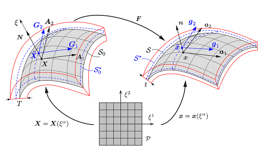
Figure 1: Mapping between parameter domain $\mathcal{P}$, reference surface $\mathcal{S}_{0}$ and current surface $\mathcal{S}$ of a Kirchhoff–Love shell. The boundaries of the physical shell are shown by solid red lines. A shell layer is denoted by $\mathcal{S}^{*}$ and $\mathcal{S}_{0}^{*}$ in the current and reference configuration, respectively, and is shown by dashed blue lines.

As shown in Fig. 1, let the mid-surface $\mathcal{S}$ of a thin shell be described by a general mapping

$$\begin{array}[]{l}\boldsymbol{x}=\boldsymbol{x}(\xi^{\alpha})~,~\alpha=1,\,2,\end{array}$$ (1)

where $\boldsymbol{x}$ denotes the surface position in 3D space and $\xi^{\alpha}$ are curvilinear coordinates embedded in the surface. They can be associated with a parameter domain $\mathcal{P}$. Differential geometry allows us to determine the co-variant tangent vectors $\boldsymbol{a}_{\alpha}=\partial{\boldsymbol{x}}/\partial\xi^{\alpha}$ on $\mathcal{S}$, their dual vectors $\boldsymbol{a}^{\alpha}$ defined by $\boldsymbol{a}^{\alpha}\cdot\boldsymbol{a}_{\beta}=\delta^{\alpha}_{\beta}$, and the surface normal $\boldsymbol{n}=(\boldsymbol{a}_{1}\times\boldsymbol{a}_{2})/||\boldsymbol{a}_{1}\times\boldsymbol{a}_{2}||$, so that the metric tensor with co-variant components $a_{\alpha\beta}=\boldsymbol{a}_{\alpha}\cdot\boldsymbol{a}_{\beta}$ and contra-variant components $[a^{\alpha\beta}]=[a_{\alpha\beta}]^{-1}$ of the first fundamental form are defined. The relation between area elements on $\mathcal{S}$ and the parameter domain is $\mathrm{d}a=J_{a}\,\mathrm{d}\xi^{1}\,\mathrm{d}\xi^{2}$ with $J_{a}=\sqrt{\det a_{\alpha\beta}}$.

The bases $\{\boldsymbol{a}_{1},\,\boldsymbol{a}_{2},\,\boldsymbol{n}\}$ and $\{\boldsymbol{a}^{1},\,\boldsymbol{a}^{2},\,\boldsymbol{n}\}$ define the usual identity tensor $\mathbf{1}$ in $\mathbb{R}^{3}$ as $\mathbf{1}=\boldsymbol{i}+\boldsymbol{n}\otimes\boldsymbol{n}$ with $\boldsymbol{i}=\boldsymbol{a}_{\alpha}\otimes\boldsymbol{a}^{\alpha}=\boldsymbol{a}^{\alpha}\otimes\boldsymbol{a}_{\alpha}$. The components of the curvature tensor $\boldsymbol{b}=b_{\alpha\beta}\,\boldsymbol{a}^{\alpha}\otimes\boldsymbol{a}^{\beta}$ are given by the Gauss–Weingarten equation

$$\begin{array}[]{l}b_{\alpha\beta}=\boldsymbol{n}\cdot\boldsymbol{a}_{\alpha,\beta}=-\boldsymbol{n}_{,\beta}\cdot\boldsymbol{a}_{\alpha}~,\end{array}$$ (2)

where a comma denotes the parametric derivative $\boldsymbol{a}_{\alpha,\beta}=\partial\boldsymbol{a}_{\alpha}/\partial\xi^{\beta}$. With the definition of the Christoffel symbol $\Gamma^{\gamma}_{\alpha\beta}=\boldsymbol{a}^{\gamma}\cdot\boldsymbol{a}_{\alpha,\beta}$, the so-called co-variant derivative is defined as $\boldsymbol{a}_{\alpha;\beta}:=\boldsymbol{a}_{\alpha,\beta}-\Gamma^{\gamma}_{\alpha\beta}\,\boldsymbol{a}_{\gamma}=(\boldsymbol{n}\otimes\boldsymbol{n})\,\boldsymbol{a}_{\alpha,\beta}$. The mean and Gaussian curvature of $\mathcal{S}$ can be computed from the first and second invariants of the curvature tensor $\boldsymbol{b}$, respectively, as

$$H:=\displaystyle\frac{1}{2}\mathrm{tr}\,{\boldsymbol{b}}=\frac{1}{2}\,b^{\alpha}_{\alpha}=\frac{1}{2}\,a^{\alpha\beta}\,b_{\alpha\beta}~,$$ (3)

and

$$\kappa:=\det{\boldsymbol{b}}=\frac{b}{a}~,$$ (4)

where

$$a=\det[a_{\alpha\beta}]~,\quad b=\det[b_{\alpha\beta}]~.$$ (5)

The variations of the above quantities such as $\delta a_{\alpha\beta}$, $\delta a^{\alpha\beta}$, $\delta b_{\alpha\beta}$, $\delta b^{\alpha\beta}$, $\delta H$ and $\delta\kappa$ can be found e.g. in Sauer and Duong, (2015).

To characterize the deformation of $\mathcal{S}$ due to loading, the initially undeformed configuration is chosen as a reference configuration and is denoted by $\mathcal{S}_{0}$. It is described by the mapping $\boldsymbol{X}=\boldsymbol{X}(\xi^{\alpha})$, from which we have $\boldsymbol{A}_{\alpha}=\partial{\boldsymbol{X}}/\partial\xi^{\alpha}$, $A_{\alpha\beta}=\boldsymbol{A}_{\alpha}\cdot\boldsymbol{A}_{\beta}$, $[A^{\alpha\beta}]=[A_{\alpha\beta}]^{-1}$, $\boldsymbol{A}^{\alpha}=A^{\alpha\beta}\,\boldsymbol{A}_{\beta}$, $\boldsymbol{N}=(\boldsymbol{A}_{1}\times\boldsymbol{A}_{2})/||\boldsymbol{A}_{1}\times\boldsymbol{A}_{2}||$, the initial identity tensor $\boldsymbol{I}:=\boldsymbol{A}_{\alpha}\otimes\boldsymbol{A}^{\alpha}=\boldsymbol{A}^{\alpha}\otimes\boldsymbol{A}_{\alpha}$, where $\mathbf{1}=\boldsymbol{I}+\boldsymbol{N}\otimes\boldsymbol{N}$, and the initial curvature tensor $\boldsymbol{b}_{0}:=B_{\alpha\beta}\,\boldsymbol{A}^{\alpha}\otimes\boldsymbol{A}^{\beta}$.

Having the definition of $a_{\alpha\beta}$ and $b_{\alpha\beta}$, the deformation map $\boldsymbol{x}=\mbox{\boldmath$\varphi$}(\boldsymbol{X})$ is fully characterized by the two following quantities:
1. The surface deformation gradient, which is defined as

$$\begin{array}[]{l}\boldsymbol{F}:=\boldsymbol{a}_{\alpha}\otimes\boldsymbol{A}^{\alpha}~.\end{array}$$ (6)

Accordingly, the right Cauchy-Green surface tensor, $\boldsymbol{C}=\boldsymbol{F}^{T}\boldsymbol{F}=a_{\alpha\beta}\,\boldsymbol{A}^{\alpha}\otimes\boldsymbol{A}^{\beta}$, its inverse $\boldsymbol{C}^{-1}=a^{\alpha\beta}\,\boldsymbol{A}_{\alpha}\otimes\boldsymbol{A}_{\beta}$, and the left Cauchy-Green surface tensor, $\boldsymbol{B}=\boldsymbol{F}\boldsymbol{F}^{T}=A^{\alpha\beta}\,\boldsymbol{a}_{\alpha}\otimes\boldsymbol{a}_{\beta}$, are defined. They have the two invariants $I_{1}=\boldsymbol{C}:\boldsymbol{I}=\boldsymbol{B}:\boldsymbol{i}=A^{\alpha\beta}\,a_{\alpha\beta}$ and $J^{2}=\det\boldsymbol{C}=\det\boldsymbol{B}$. Therefore, similar to the volumetric case, the surface Green-Lagrange strain tensor can be defined as

$$\begin{array}[]{l}\boldsymbol{E}=E_{\alpha\beta}\,\boldsymbol{A}^{\alpha}\otimes\boldsymbol{A}^{\beta}:=\displaystyle\frac{1}{2}(\boldsymbol{C}-\boldsymbol{I})=\displaystyle\frac{1}{2}(a_{\alpha\beta}-A_{\alpha\beta})\,\boldsymbol{A}^{\alpha}\otimes\boldsymbol{A}^{\beta}~,\end{array}$$ (7)

which represents the change of the metric tensor due to the surface deformation.
2. The symmetric relative curvature tensor, which is defined as

$$\begin{array}[]{l}\boldsymbol{K}=K_{\alpha\beta}\,\boldsymbol{A}^{\alpha}\otimes\boldsymbol{A}^{\beta}:=\boldsymbol{\kappa}-\boldsymbol{b}_{0}=(b_{\alpha\beta}-B_{\alpha\beta})\,\boldsymbol{A}^{\alpha}\otimes\boldsymbol{A}^{\beta},\end{array}$$ (8)

with

$$\begin{array}[]{l}\boldsymbol{\kappa}:=\boldsymbol{F}^{T}\,\boldsymbol{b}\,\boldsymbol{F}=b_{\alpha\beta}\,\boldsymbol{A}^{\alpha}\otimes\boldsymbol{A}^{\beta}~,\end{array}$$ (9)

which furnishes the change of the curvature tensor field, following the terminology of Steigmann, 1999b .

2.2 Stress and moment tensors

In order to define stresses at a material point $\boldsymbol{x}$ of the shell surface $\mathcal{S}$, the shell is cut into two at $\boldsymbol{x}$ by the parametrized curve $\mathcal{C}(s)$. Further, let $\mbox{\boldmath$\tau$}:=\partial\boldsymbol{x}/\partial s$ be the unit tangent and $\mbox{\boldmath$\nu$}:=\mbox{\boldmath$\tau$}\times\boldsymbol{n}$ be the unit normal of $\mathcal{C}$ at $\boldsymbol{x}$. Then, one can define the traction vector $\boldsymbol{T}=\boldsymbol{T}^{\alpha}\,\nu_{\alpha}$ and the moment vector $\boldsymbol{M}=\boldsymbol{M}^{\alpha}\,\nu_{\alpha}$ on each side of $\mathcal{C}(s)$ at $\boldsymbol{x}$, where $\nu_{\alpha}=\mbox{\boldmath$\nu$}\cdot\boldsymbol{a}_{\alpha}$. According to Cauchy’s theorem, these vectors can be linearly mapped to the normal $\nu$ by second order tensors as

$$\begin{array}[]{lll}\boldsymbol{T}:=\mbox{\boldmath$\sigma$}^{\mathrm{T}}\mbox{\boldmath$\nu$}~,\\[5.69054pt] \boldsymbol{M}:=\boldsymbol{\mu}^{\mathrm{T}}\,\mbox{\boldmath$\nu$}~,\end{array}$$ (10)

where

$$\begin{array}[]{lll}\mbox{\boldmath$\sigma$}:=N^{\alpha\beta}\,\boldsymbol{a}_{\alpha}\otimes\boldsymbol{a}_{\beta}+S^{\alpha}\,\boldsymbol{a}_{\alpha}\otimes\boldsymbol{n}~,\\[5.69054pt] \boldsymbol{\mu}:=-M^{\alpha\beta}\,\boldsymbol{a}_{\alpha}\otimes\boldsymbol{a}_{\beta}\end{array}$$ (11)

are the Cauchy stress and moment tensors, respectively.

It should be noted that the Cauchy stress $\sigma$ in Eq. (11.1) is generally not symmetric. Furthermore, as shown e.g. in Sauer and Duong, (2015), a suitable work conjugation (per reference area) arising in the presented theory is the quartet

$$\begin{array}[]{l}\dot{W}_{\mathrm{int}}:=\ \tau^{\alpha\beta}\dot{a}_{\alpha\beta}/2+M^{\alpha\beta}_{0}\dot{b}_{\alpha\beta}~,\end{array}$$ (12)

where $\dot{W}_{\mathrm{int}}$ is the local power density and we have defined

$$\begin{array}[]{lll}\tau^{\alpha\beta}\!\!\!&:=&\!\!\!J\sigma^{\alpha\beta}~,\\[2.84526pt] M_{0}^{\alpha\beta}\!\!\!&:=&\!\!\!JM^{\alpha\beta}~.\end{array}$$ (13)

Further,

$$\begin{array}[]{lll}\sigma^{\alpha\beta}:=N^{\alpha\beta}-b^{\beta}_{\gamma}\,M^{\gamma\alpha}\end{array}$$ (14)

are the components of the membrane stress responding to the change of the metric tensor.

We also note that the mathematical quantities introduced in Eqs. (10) and (11) stem from the Cosserat theory for thin shells (Steigmann, 1999b, ). As shown e.g. by Steigmann, 1999a and Sauer and Duong, (2015), these quantities can be related to the effective traction $\boldsymbol{t}$ and physical moment $\boldsymbol{m}$ transmitted across $\mathcal{C}(s)$. Namely for $\boldsymbol{m}$, the relation is given by

$$\begin{array}[]{l}\boldsymbol{m}:=\boldsymbol{n}\times\boldsymbol{M}=m_{\nu}\,\mbox{\boldmath$\nu$}+m_{\tau}\,\mbox{\boldmath$\tau$},\end{array}$$ (15)

where

$$\begin{array}[]{lll}m_{\nu}\!\!\!&:=&\!\!\!M^{\alpha\beta}\,\nu_{\alpha}\,\tau_{\beta}~,\\[2.84526pt] m_{\tau}\!\!\!&:=&\!\!\!-M^{\alpha\beta}\,\nu_{\alpha}\,\nu_{\beta}~,\end{array}$$ (16)

are the normal and tangential bending moment components along $\mathcal{C}(s)$. For the effective traction $\boldsymbol{t}$, one can show that (Steigmann, 1999b, ; Sauer and Duong,, 2015)

$$\begin{array}[]{l}\boldsymbol{t}:=\boldsymbol{T}-\left(m_{\nu}\,\boldsymbol{n}\right)^{\prime}~,\end{array}$$ (17)

where $(\bullet)^{\prime}$ denotes the derivative with respect to $s$.

2.3 Balance laws

To derive the governing equations, the surface $\mathcal{S}$ is subjected to the prescribed body force $\boldsymbol{f}=f^{\alpha}\,\boldsymbol{a}_{\alpha}+p\,\boldsymbol{n}$ on $\mathcal{S}$ and the boundary conditions

$$\begin{array}[]{rllll}\boldsymbol{u}\!\!\!&=&\!\!\!\bar{\boldsymbol{u}}&$on$~\partial_{u}\mathcal{S}~,\\[2.84526pt] \boldsymbol{n}\!\!\!&=&\!\!\!\bar{\boldsymbol{n}}&$on$~\partial_{n}\mathcal{S}~,\\[2.84526pt] \boldsymbol{t}\!\!\!&=&\!\!\!\bar{\boldsymbol{t}}&$on$~\partial_{t}\mathcal{S}~,\\[2.84526pt] m_{\tau}\!\!\!&=&\!\!\!\bar{m}_{\tau}&$on$~\partial_{m}\mathcal{S}~,\end{array}$$ (18)

where $\bar{\boldsymbol{u}}$ is a prescribed displacement; $\bar{\boldsymbol{n}}$ is a prescribed rotation, $\bar{\boldsymbol{t}}:=\bar{t}^{\alpha}\,\boldsymbol{a}_{\alpha}$ is a prescribed boundary traction and $\bar{m}_{\tau}$ is a prescribed bending moment. The equilibrium of the shell is then governed by the balance of linear momentum together with mass conservation, which gives

$$\begin{array}[]{lll}\boldsymbol{T}^{\alpha}_{;\alpha}+\boldsymbol{f}=\rho\,\dot{\boldsymbol{v}}\quad\forall\,\boldsymbol{x}\in\mathcal{S}~,\end{array}$$ (19)

while the balance of angular momentum leads to the condition that $\sigma^{\alpha\beta}$, defined in Eq. (14), is symmetric and the shear stress is related to the bending moment via

$$\begin{array}[]{lll}S^{\alpha}=-M^{\beta\alpha}_{~~;\beta}~.\end{array}$$ (20)

We note that $M^{\alpha\beta}$ is also symmetric but $N^{\alpha\beta}$ is generally not symmetric.

2.4 Weak form

The weak form of Eq. (19) can be obtained by contracting Eq. (19) with the admissible variation $\delta\boldsymbol{x}\in\mathcal{V}$ and integrating over $\mathcal{S}$, (see Sauer and Duong, (2015)). This results in

$$\begin{array}[]{l}G_{\mathrm{in}}+G_{\mathrm{int}}-G_{\mathrm{ext}}=0\quad\forall\,\delta\boldsymbol{x}\in\mathcal{V}~,\end{array}$$ (21)

where

$$\begin{array}[]{lll}G_{\mathrm{in}}\!\!\!&=&\!\!\!\displaystyle\int_{\mathcal{S}_{0}}\delta\boldsymbol{x}\cdot\rho_{0}\,\dot{\boldsymbol{v}}\,\mathrm{d}A~,\\[11.38109pt] G_{\mathrm{int}}\!\!\!&=&\!\!\!\displaystyle\int_{\mathcal{S}_{0}}\frac{1}{2}\,\delta a_{\alpha\beta}\,\tau^{\alpha\beta}\,\mathrm{d}A+\int_{\mathcal{S}_{0}}\delta b_{\alpha\beta}\,M_{0}^{\alpha\beta}\,\mathrm{d}A~=\displaystyle\int_{\mathcal{S}_{0}}\delta E_{\alpha\beta}\,\tau^{\alpha\beta}\,\mathrm{d}A+\int_{\mathcal{S}_{0}}\delta K_{\alpha\beta}\,M_{0}^{\alpha\beta}\,\mathrm{d}A~,\\[11.38109pt] G_{\mathrm{ext}}\!\!\!&=&\!\!\!\displaystyle\int_{\mathcal{S}}\delta\boldsymbol{x}\cdot\boldsymbol{f}\,\mathrm{d}a+\displaystyle\int_{\partial_{t}\mathcal{S}}\delta\boldsymbol{x}\cdot\boldsymbol{t}\,\mathrm{d}s+\displaystyle\int_{\partial_{m}\mathcal{S}}\delta\boldsymbol{n}\cdot m_{\tau}\,\mbox{\boldmath$\nu$}\,\mathrm{d}s+[\delta\boldsymbol{x}\cdot m_{\nu}\,\boldsymbol{n}\big{]}~.\end{array}$$ (22)

Remark 1: Here, the last term in $G_{\mathrm{ext}}$ is the virtual work of the point load $m_{\nu}\,\boldsymbol{n}$ at corners of $\partial_{m}\mathcal{S}$ (in case $m_{\nu}\neq 0$), and the second last term in $G_{\mathrm{ext}}$ denotes the virtual work of the moment $m_{\tau}\,\mbox{\boldmath$\nu$}$. It is worth noting that this is the consistent way to apply bending moments on the boundary of Kirchhoff–Love shells.

2.5 Linearization of the weak form

For solving the nonlinear equation (21) by the Newton–Raphson method, its linearization is needed. For the kinetic virtual work, one gets

$$\begin{array}[]{lll}\Delta G_{\mathrm{in}}\!\!\!&=&\!\!\!\displaystyle\int_{\mathcal{S}_{0}}\delta\boldsymbol{x}\cdot\rho_{0}\,\Delta\dot{\boldsymbol{v}}\,\mathrm{d}A~,\end{array}$$ (23)

in which $\Delta\dot{\boldsymbol{v}}$ depends on the time integration scheme used. For dead loading of $\boldsymbol{f}$, $\boldsymbol{t}$ and $m_{\tau}\,\mbox{\boldmath$\nu$}$, one finds

$$\begin{array}[]{l}\Delta G_{\mathrm{ext}}=\displaystyle\int_{\partial\mathcal{S}}m_{\tau}\,\delta\boldsymbol{a}_{\alpha}\cdot\big{(}\nu^{\beta}\,\boldsymbol{n}\otimes\boldsymbol{a}^{\alpha}+\nu^{\alpha}\,\boldsymbol{a}^{\beta}\otimes\boldsymbol{n}\big{)}\,\Delta\boldsymbol{a}_{\beta}\,\mathrm{d}s\end{array}$$ (24)

and for the internal virtual work term

$$\begin{array}[]{llllll}\Delta G_{\mathrm{int}}=\displaystyle\int_{\mathcal{S}_{0}}\Big{(}\hskip-8.61108pt&c^{\alpha\beta\gamma\delta}\,\frac{1}{2}\delta a_{\alpha\beta}\,\frac{1}{2}\Delta a_{\gamma\delta}\!\!\!&+&\!\!\!d^{\alpha\beta\gamma\delta}\,\frac{1}{2}\delta a_{\alpha\beta}\,\Delta b_{\gamma\delta}\!\!\!&+&\!\!\!\tau^{\alpha\beta}\,\frac{1}{2}\Delta\delta a_{\alpha\beta}\;+\\[8.53581pt] &e^{\alpha\beta\gamma\delta}\,\delta b_{\alpha\beta}\,\frac{1}{2}\Delta a_{\gamma\delta}\!\!\!&+&\!\!\!f^{\alpha\beta\gamma\delta}\,\delta b_{\alpha\beta}\,\Delta b_{\gamma\delta}\!\!\!&+&\!\!\!M^{\alpha\beta}_{0}\,\Delta\delta b_{\alpha\beta}\Big{)}\,\mathrm{d}A~,\end{array}$$ (25)

where the material tangent matrices are defined as

$$\begin{array}[]{lllll}c^{\alpha\beta\gamma\delta}\!\!\!&:=&\!\!\!2\displaystyle\frac{\partial\tau^{\alpha\beta}}{\partial a_{\gamma\delta}}~,\quad~d^{\alpha\beta\gamma\delta}\!\!\!&:=&\!\!\!\displaystyle\frac{\partial\tau^{\alpha\beta}}{\partial b_{\gamma\delta}}~,\\[5.69054pt] e^{\alpha\beta\gamma\delta}\!\!\!&:=&\!\!\!2\displaystyle\frac{\partial M_{0}^{\alpha\beta}}{\partial a_{\gamma\delta}}~,\quad f^{\alpha\beta\gamma\delta}\!\!\!&:=&\!\!\!\displaystyle\frac{\partial M_{0}^{\alpha\beta}}{\partial b_{\gamma\delta}}~.\end{array}$$ (26)

They are given in Sauer and Duong, (2015) for various material models. Here it is noted that $d^{\alpha\beta\gamma\delta}=e^{\gamma\delta\alpha\beta}$ posses minor symmetries, while $c^{\alpha\beta\gamma\delta}$ and $f^{\alpha\beta\gamma\delta}$ posses both minor and major symmetries.

2.6 Constitution

In this framework, $\sigma^{\alpha\beta}$ and $M^{\alpha\beta}$ are determined from constitutive relations for stretching and bending. For hyperelastic shells, we assume there exists a stored energy function in the form

$$\begin{array}[]{l}W=W(\boldsymbol{E},\boldsymbol{K}),\end{array}$$ (27)

where $\boldsymbol{E}$ and $\boldsymbol{K}$ are defined in Eqs. (7) and (8). The Koiter model (see Eq. (35)) is a simple example of this form. It is easily seen that $W$ can be equivalently expressed as a function of $\boldsymbol{C}$ and $\boldsymbol{\kappa}$, or as a function of $a_{\alpha\beta}$ and $b_{\alpha\beta}$, since $\boldsymbol{A}^{\alpha}$ is constant. If the material has symmetries, e.g. isotropy, the stored energy function can also be expressed as a function of the invariants $I_{1}$, $J$, $H$ and $\kappa$, defined in Sec. 2.1 (see e.g. Steigmann, 1999a ). Thus, the following functional forms are equivalent to Eq. (27).

$$\begin{array}[]{l}W=W(\boldsymbol{C},\boldsymbol{\kappa})=W(a_{\alpha\beta},b_{\alpha\beta})=W(I_{1},J,H,\kappa)~.\end{array}$$ (28)

Given the stored energy function $W$, the common argument by Coleman and Noll, (1964) leads to the constitutive equations (see Sauer and Duong, (2015))

$$\begin{array}[]{llrlrlr}\tau^{\alpha\beta}\!\!\!&=&\!\!\!\displaystyle 2\,\frac{\partial{W}}{\partial{a_{\alpha\beta}}}~,\\[11.38109pt] M_{0}^{\alpha\beta}\!\!\!&=&\!\!\!\displaystyle\frac{\partial{W}}{\partial{b_{\alpha\beta}}}~.\end{array}$$ (29)

Remark 2: The constitutive equations (29) are defined in curvilinear coordinates. Therefore, they either give the components of the classical second Piola-Kirchhoff stress and moment

$$\begin{array}[]{lll}\boldsymbol{S}\!\!\!&:=&\!\!\!\displaystyle\frac{\partial{W(\boldsymbol{E},\boldsymbol{K})}}{\partial{\boldsymbol{E}}}=\displaystyle 2\,\frac{\partial{W}}{\partial{a_{\alpha\beta}}}\,\boldsymbol{A}_{\alpha}\otimes\boldsymbol{A}_{\beta}=:\tau^{\alpha\beta}\,\boldsymbol{A}_{\alpha}\otimes\boldsymbol{A}_{\beta}~,\\[11.38109pt] \boldsymbol{{\mu}_{0}}\!\!\!&:=&\!\!\!-\displaystyle\frac{\partial{W(\boldsymbol{E},\boldsymbol{K})}}{\partial{\boldsymbol{\boldsymbol{K}}}}=-\displaystyle\frac{\partial{W}}{\partial{b_{\alpha\beta}}}\,\boldsymbol{A}_{\alpha}\otimes\boldsymbol{A}_{\beta}=:-M_{0}^{\alpha\beta}\,\boldsymbol{A}_{\alpha}\otimes\boldsymbol{A}_{\beta},\end{array}$$ (30)

of the surface manifold. Alternatively, they give the components of the Kirchhoff stress and moment defined by pushing forward $\boldsymbol{S}$ and $\boldsymbol{{\mu}_{0}}$ as

$$\begin{array}[]{lll}\boldsymbol{F}\,\boldsymbol{S}\,\boldsymbol{F}^{T}\!\!\!&:=&\!\!\!\tau^{\alpha\beta}\,\boldsymbol{a}_{\alpha}\otimes\boldsymbol{a}_{\beta}~,\\[11.38109pt] \boldsymbol{F}\,\boldsymbol{\mu_{0}}\,\boldsymbol{F}^{T}\!\!\!&:=&\!\!\!-M_{0}^{\alpha\beta}\,\boldsymbol{a}_{\alpha}\otimes\boldsymbol{a}_{\beta}=J\,\boldsymbol{\mu}.\end{array}$$ (31)

Here, we note that $\frac{\partial{(\bullet)}}{\partial{\boldsymbol{X}}}$ in Eq. (30) denotes the derivative of a scalar-valued function by an arbitrary second order tensor $\boldsymbol{X}$ (see e.g. Itskov, (2009)).

Remark 3: In this framework, the stress $\sigma^{\alpha\beta}$ and moment $M^{\alpha\beta}$ are both constitutively determined from a surface stored energy function $W$. The advantage of this setup is that it can accept general constitutive relations, which implies that the relation between the membrane and bending response can be flexibly realized at the constitutive level and it is not restricted within the formulation. The stretching and bending response may range from fully decoupled, like in the Koiter material model (Eq. (35)), to a coupled relation, such as in the Helfrich material model (see e.g. Sauer and Duong, (2015)). Due to this flexibility, the presented formulation is suitable for both solid and liquid shells and is also convenient for adding kinematic constraints (e.g. area constraint) or stabilization potentials (Sauer et al.,, 2017).

Remark 4: In the presented formulation, we note that the definition of the shell thickness is not needed for solving Eq. (21), which is often referred to as a “zero-thickness” formulation. Consequently, the stress and moment in Eq. (29) can be computed without defining a thickness. However, this does not imply that thickness effects have been neglected or approximated. Instead, they are in some sense hidden in the constitutive law of Eq. (27). If desired, they can be determined as noted in Remark 2.6.2. But this connection is not a requirement as it is in the case of constitutive laws derived from 3D material models (see Sec. 3.4).

In the following, we consider some example constitutive models suitable for solid shells to demonstrate the flexibility of the formulation. The application of the formulation to liquid shells is considered in future work (Sauer et al.,, 2017).

2.6.1 Initially planar shells

For initially planar shells, one can consider the model of Canham, (1970) for the bending contribution, while for the membrane contribution, the stretching response can be modeled with a nonlinear Neo-Hookean law. This gives

$$\begin{array}[]{l}W=\displaystyle\frac{\Lambda}{4}(J^{2}-1-2\ln J)+\displaystyle\frac{\mu}{2}(I_{1}-2-2\ln J)+\displaystyle c\,J\,\big{(}2\,H^{2}-\kappa\big{)}~,\end{array}$$ (32)

where $c$, $\Lambda$ and $\mu$ are 2D material constants. From Eqs. (29) and (32), we find the stress

$$\begin{array}[]{l}\tau^{\alpha\beta}=\displaystyle\frac{\Lambda}{2}\big{(}J^{2}-1\big{)}a^{\alpha\beta}+\mu\Big{(}A^{\alpha\beta}-a^{\alpha\beta}\Big{)}+c\,J\,(2H^{2}+\kappa)\,a^{\alpha\beta}-4c\,J\,H\,b^{\alpha\beta}~,\end{array}$$ (33)

and the moment

$$\begin{array}[]{l}M^{\alpha\beta}_{0}=c\,J\,b^{\alpha\beta}~,\end{array}$$ (34)

which is linear w.r.t. the curvature. The tangents for this are given in Sauer and Duong, (2015). We note that since Eq. (32) is given in surface strain energy form, the stress and moment can be computed directly from Eqs. (33) and (34) without needing any thickness integration.

2.6.2 Initially curved solid shell

For initially curved shells, the surface strain energy model proposed by Koiter (Ciarlet,, 2005; Steigmann,, 2013) can be considered. It is defined in tensor notation as

$$\begin{array}[]{l}W(\boldsymbol{E},\boldsymbol{K})=\displaystyle\frac{1}{2}\,\boldsymbol{E}:\mathbb{C}:\boldsymbol{E}+\displaystyle\frac{1}{2}\,\boldsymbol{K}:\mathbb{F}:\boldsymbol{K}~,\end{array}$$ (35)

with the constant fourth order tensors

$$\begin{array}[]{lll}\mathbb{C}\!\!\!&=&\!\!\!\Lambda\,\boldsymbol{I}\odot\boldsymbol{I}+2\,\mu\,(\boldsymbol{I}\otimes\boldsymbol{I})^{\mathrm{s}}~,\\[5.69054pt] \mathbb{F}\!\!\!&=&\!\!\!\displaystyle\frac{T^{2}}{12}\,\mathbb{C}~.\end{array}$$ (36)

Since $\boldsymbol{I}\odot\boldsymbol{I}:\boldsymbol{X}=(\mathrm{tr}\,\boldsymbol{X})\,\boldsymbol{I}$ and $(\boldsymbol{I}\otimes\boldsymbol{I})^{\mathrm{s}}:\boldsymbol{X}=\mathrm{sym}(\boldsymbol{X})$, with $\boldsymbol{X}$ being an arbitrary second order tensor, it follows from Eqs. (35) and (36) that

$$\begin{array}[]{lll}\tau^{\alpha\beta}\!\!\!&=&\!\!\!\Lambda\,\mathrm{tr}\,\boldsymbol{E}\,A^{\alpha\beta}+2\,\mu\,E^{\alpha\beta}~,\\[5.69054pt] M_{0}^{\alpha\beta}\!\!\!&=&\!\!\!\displaystyle\frac{T^{2}}{12}(\Lambda\,\mathrm{tr}\,\boldsymbol{K}\,A^{\alpha\beta}+2\,\mu\,K^{\alpha\beta}),\end{array}$$ (37)

where $K^{\alpha\beta}:=A^{\alpha\gamma}\,K_{\gamma\delta}\,A^{\delta\beta}$, $E^{\alpha\beta}:=A^{\alpha\gamma}\,E_{\gamma\delta}\,A^{\delta\beta}$, and

$$\begin{array}[]{lll}\mathrm{tr}\,\boldsymbol{K}=K^{\alpha\beta}\,A_{\alpha\beta}~,\quad\mathrm{tr}\,\boldsymbol{E}=E^{\alpha\beta}\,A_{\alpha\beta}~.\end{array}$$ (38)

From Eq. (37), we further find $d^{\alpha\beta\gamma\delta}=e^{\alpha\beta\gamma\delta}=0$ and

$$\begin{array}[]{lllll}c^{\alpha\beta\gamma\delta}\!\!\!&=&\!\!\!\Lambda\,A^{\alpha\beta}\,A^{\gamma\delta}+\mu\big{(}A^{\alpha\gamma}\,A^{\beta\delta}+A^{\alpha\delta}\,A^{\beta\gamma}\big{)}~,\\[5.69054pt] f^{\alpha\beta\gamma\delta}\!\!\!&=&\!\!\!\displaystyle\frac{T^{2}}{12}\,c^{\alpha\beta\gamma\delta}~.\end{array}$$ (39)

Remark 5: The set of parameters $\Lambda$ and $\mu$ can be determined in different ways. Firstly, they can be determined directly from experiments, i.e. without explicitly considering the thickness. Secondly, they may be obtained by analytical integration over the thickness of the simple 3D Saint Venant–Kirchhoff model (see e.g. Ciarlet, (2005) and Sec. 3.4). In this case, $\mu$ and $\Lambda$ are given by

$$\begin{array}[]{lll}\Lambda:=\displaystyle T\,\frac{2\,\tilde{\Lambda}\,\tilde{\mu}}{\tilde{\Lambda}+2\,\tilde{\mu}},\quad\mu:=T\,\tilde{\mu},\end{array}$$ (40)

where $\tilde{\Lambda}$ and $\tilde{\mu}$ are the classical 3D Lamé constants in linear elasticity. Thirdly, they can be determined by numerical integration over the thickness of a general 3D material model.

Remark 6: Note that, in Eq. (35), the stretching and the bending behavior can be specified separately. For instance, the first term can be replaced by a nonlinear Neo-Hooke model (see Eq. (32)), i.e.

$$\begin{array}[]{l}W=\displaystyle\frac{\Lambda}{4}(J^{2}-1-2\ln J)+\displaystyle\frac{\mu}{2}(I_{1}-2-2\ln J)+\displaystyle\frac{1}{2}\,\boldsymbol{K}:\mathbb{F}:\boldsymbol{K}~,\end{array}$$ (41)

in order to capture large membrane strains. In this case $\tau^{\alpha\beta}$ follows from the front part of Eq. (33), while $M_{0}^{\alpha\beta}$ is given by Eq. (37.2).

3 Shell constitution derived from 3D constitutive laws

Provided the displacement across the shell thickness complies with the Kirchhoff–Love assumption, a constitutive relation $W=W(\boldsymbol{E},\boldsymbol{K})$ for shells can also be extracted, without approximation, from classical three-dimensional constitutive models of the form $\tilde{W}=\tilde{W}(\tilde{\boldsymbol{C}})$, where $\tilde{\boldsymbol{C}}$ is the right Cauchy-Green tensor for 3D continua. This procedure corresponds to a projection of 3D models onto surface $\mathcal{S}$, or to an extraction of 2D surface models out of 3D ones. This approach goes back to Hughes and Carnoy, (1983); De Borst, (1991); Dvorkin et al., (1995); Klinkel and Govindjee, (2002); Kiendl et al., 2015b , and it is presented here to show how it relates to our formulation.

3.1 Extraction procedure

As shown in Fig. 1, a shell material point $P$ can be described w.r.t. the mid-surface in the reference configuration as (Wriggers,, 2008)

$$\begin{array}[]{l}\tilde{\boldsymbol{X}}(\xi^{\alpha},\xi_{0})=\boldsymbol{X}(\xi^{\alpha})+\xi_{0}\,\boldsymbol{N}(\xi^{\alpha})~,\end{array}$$ (42)

and in the current configuration as

$$\begin{array}[]{l}\tilde{\boldsymbol{x}}(\xi^{\alpha},\,\xi)=\boldsymbol{x}(\xi^{\alpha})+\xi\,\boldsymbol{d}(\xi^{\alpha})~,\end{array}$$ (43)

where $\xi_{0}\in[-T/2,\,T/2]$ is the thickness coordinate of the shell and $\boldsymbol{d}$ is the director vector which has three unknown components in general. For Kirchhoff–Love theory, which is considered here, $\boldsymbol{d}:=\boldsymbol{n}$ and $\xi=\lambda_{3}\,\xi_{0}$, where $\lambda_{3}$ denotes the stretch in the normal direction. Thus, the tangent vectors at $P$ are expressed w.r.t. the basis formed by the tangent vectors on the mid-surface as

$$\begin{array}[]{llll}\boldsymbol{g}_{\alpha}\!\!\!&:=&\!\!\!\tilde{\boldsymbol{x}}_{,\alpha}=\boldsymbol{a}_{\alpha}-\xi\,b_{\alpha}^{\gamma}\,\boldsymbol{a}_{\gamma}~,\\[5.69054pt] \boldsymbol{g}_{3}\!\!\!&:=&\!\!\!\tilde{\boldsymbol{x}}_{,\xi}=\boldsymbol{d}~,\\[5.69054pt] \boldsymbol{G}_{\alpha}\!\!\!&:=&\!\!\!\tilde{\boldsymbol{X}}_{,\alpha}=\boldsymbol{A}_{\alpha}-\xi_{0}\,B_{\alpha}^{\gamma}\,\boldsymbol{A}_{\gamma}~,\\[5.69054pt] \boldsymbol{G}_{3}\!\!\!&:=&\!\!\!\tilde{\boldsymbol{X}}_{,{\xi_{0}}}=\boldsymbol{N}=\boldsymbol{G}^{3}~,\end{array}$$ (44)

and the metric tensors at $P$ can also be expressed in terms of the metric tensors on the mid-surface as

$$\begin{array}[]{llll}g_{\alpha\beta}\!\!\!&:=&\!\!\!\boldsymbol{g}_{\alpha}\cdot\boldsymbol{g}_{\beta}=g_{a}\,a_{\alpha\beta}+g_{b}\,b_{\alpha\beta}~,\\[11.38109pt] g^{\alpha\beta}\!\!\!&:=&\!\!\!\boldsymbol{g}^{\alpha}\cdot\boldsymbol{g}^{\beta}=g^{a}\,a^{\alpha\beta}+g^{b}\,b^{\alpha\beta}~,\\[11.38109pt] G_{\alpha\beta}\!\!\!&:=&\!\!\!\boldsymbol{G}_{\alpha}\cdot\boldsymbol{G}_{\beta}=G_{A}\,A_{\alpha\beta}+G_{B}\,B_{\alpha\beta}~,\\[11.38109pt] G^{\alpha\beta}\!\!\!&:=&\!\!\!\boldsymbol{G}^{\alpha}\cdot\boldsymbol{G}^{\beta}=G^{A}\,A^{\alpha\beta}+G^{B}\,B^{\alpha\beta}~,\end{array}$$ (45)

where $\boldsymbol{g}^{\alpha}=g^{\alpha\beta}\,\boldsymbol{g}_{\beta}$, $[g^{\alpha\beta}]=[g_{\alpha\beta}]^{-1}$ and likewise $\boldsymbol{G}^{\alpha}$. Due to Eq. (44), the coefficients in Eq. (45) are found to be

$$\begin{array}[]{lllll}g_{a}\!\!\!&:=&\!\!\!1-\xi^{2}\,\kappa~,\quad\quad g_{b}\!\!\!&:=&\!\!\!-2\,\xi+2\,H\,\xi^{2}~,\\[8.53581pt] G_{A}\!\!\!&:=&\!\!\!1-\xi_{0}^{2}\,\kappa_{0}~,\hfill G_{B}\!\!\!&:=&\!\!\!-2\,\xi_{0}+2\,H_{0}\,\xi_{0}^{2}~,\end{array}$$ (46)

and

$$\begin{array}[]{lllll}g^{a}\!\!\!&:=&\!\!\!s^{-2}\,(g_{a}+2\,H\,g_{b})~,\quad\quad\quad g^{b}\!\!\!&:=&\!\!\!-s^{-2}\,g_{b}~,\\[8.53581pt] G^{A}\!\!\!&:=&\!\!\!s_{0}^{-2}\,(G_{A}+2\,H_{0}\,G_{B})~,\hfill G^{B}\!\!\!&:=&\!\!\!-s_{0}^{-2}\,G_{B}~.\end{array}$$ (47)

Here,

$$\begin{array}[]{llll}s:=\displaystyle\sqrt{g/a}=1-2\,H\,\xi+\kappa\,\xi^{2}~,\quad s_{0}:=\displaystyle\sqrt{G/A}=1-2\,H_{0}\,\xi_{0}+\kappa_{0}\,\xi_{0}^{2}~,\end{array}$$ (48)

denote the so-called shifters, which are the determinants of the shifting tensors $\boldsymbol{i}-\xi\,\boldsymbol{b}$ and $\boldsymbol{I}-\xi_{0}\,\boldsymbol{B}$, respectively, and we have defined

$$\begin{array}[]{l}G:=\det[G_{\alpha\beta}],\quad A:=\det[A_{\alpha\beta}],\quad B:=\det[B_{\alpha\beta}],\quad g:=\det[g_{\alpha\beta}]~.\end{array}$$ (49)

From Eqs. (46), (47), and (48), we thus find the variations (considering $\xi$ fixed)

$$\begin{array}[]{lll}\delta g_{a}\!\!\!&=&\!\!\!\xi^{2}\,\kappa\,a^{\gamma\delta}\,\delta a_{\gamma\delta}-\xi^{2}\,\tilde{b}^{\gamma\delta}\,\delta b_{\gamma\delta}~,\\[5.69054pt] \delta g_{b}\!\!\!&=&\!\!\!-\xi^{2}\,b^{\gamma\delta}\,\delta a_{\gamma\delta}+\xi^{2}\,a^{\gamma\delta}\,\delta b_{\gamma\delta}~,\end{array}$$ (50)

where $\tilde{b}^{\alpha\beta}:=2\,H\,a^{\alpha\beta}-b^{\alpha\beta}$. With these we get

$$\begin{array}[]{llll}\delta g_{\alpha\beta}=g_{a}\,\delta a_{\alpha\beta}+g_{b}\,\delta b_{\alpha\beta}+a_{\alpha\beta}\,\delta g_{a}+b_{\alpha\beta}\,\delta g_{b}~.\end{array}$$ (51)

Further, we can represent the right 3D Cauchy-Green tensor w.r.t. the basis $\{\boldsymbol{G}^{1},~\boldsymbol{G}^{2},~\boldsymbol{N}\}$ as (e.g. see Wriggers, (2008))

$$\begin{array}[]{l}\tilde{\boldsymbol{C}}=\tilde{C}_{\alpha\beta}\,\boldsymbol{G}^{\alpha}\otimes\boldsymbol{G}^{\beta}+\tilde{C}_{\alpha 3}\,\big{(}\boldsymbol{G}^{\alpha}\otimes\boldsymbol{N}+\boldsymbol{N}\otimes\boldsymbol{G}^{\alpha}\big{)}+\tilde{C}_{33}\,\boldsymbol{N}\otimes\boldsymbol{N}~.\end{array}$$ (52)

We note here that $\boldsymbol{G}_{\alpha}$ accounts for the surface stretch due to the initial shell curvature (see Eq. (44.3)) and the basis $\{\boldsymbol{G}^{1},~\boldsymbol{G}^{2},~\boldsymbol{N}\}$ on a shell layer at $\xi$ defines the usual identity tensor in $\mathbb{R}^{3}$ as

$$\begin{array}[]{l}\mathbf{1}=\boldsymbol{I}+\boldsymbol{N}\otimes\boldsymbol{N}~,\quad\boldsymbol{I}:=\boldsymbol{G}^{\alpha}\otimes\boldsymbol{G}_{\alpha}=\boldsymbol{A}^{\alpha}\otimes\boldsymbol{A}_{\alpha}.\end{array}$$ (53)

Further, the 3D Kirchhoff stress tensor can be written as

$$\begin{array}[]{l}\tilde{}\mbox{\boldmath$\tau$}=\tilde{\tau}^{\alpha\beta}\,\boldsymbol{g}_{\alpha}\otimes\boldsymbol{g}_{\beta}+\tilde{\tau}^{\alpha 3}\,\big{(}\boldsymbol{g}_{\alpha}\otimes\boldsymbol{g}_{3}+\boldsymbol{g}_{3}\otimes\boldsymbol{g}_{\alpha}\big{)}+\tilde{\tau}^{33}\,\boldsymbol{g}_{3}\otimes\boldsymbol{g}_{3}~.\end{array}$$ (54)

For the Kirchhoff–Love shell we have $\tilde{C}_{\alpha\beta}=g_{\alpha\beta}$, while $\tilde{C}_{\alpha 3}=g_{\alpha 3}=\boldsymbol{g}_{\alpha}\cdot\boldsymbol{g}_{3}=0$ and $\tilde{C}_{33}=\lambda_{3}^{2}$. Thus the variation of $\tilde{\boldsymbol{C}}$ is

$$\begin{array}[]{l}\delta\tilde{\boldsymbol{C}}=\delta{\boldsymbol{C}}^{*}+2\,\lambda_{3}\,\delta\lambda_{3}\,\boldsymbol{N}\otimes\boldsymbol{N}~,\quad\quad\boldsymbol{C}^{*}:=g_{\alpha\beta}\,\boldsymbol{G}^{\alpha}\otimes\boldsymbol{G}^{\beta}~.\end{array}$$ (55)

With this, the total strain energy of the shell can be expressed w.r.t. the mid-surface as

$$\begin{array}[]{l}\mathcal{W}=\displaystyle\int_{\Omega_{0}}\tilde{W}\mathrm{d}V=\displaystyle\int_{\mathcal{S}_{0}}\int_{-\frac{T}{2}}^{\frac{T}{2}}\tilde{W}\,\mathrm{d}\xi_{0}\,\mathrm{d}G=\displaystyle\int_{\mathcal{S}_{0}}\int_{-\frac{T}{2}}^{\frac{T}{2}}s_{0}\,\tilde{W}\,\mathrm{d}\xi_{0}\,\mathrm{d}A~,\end{array}$$ (56)

where $\mathrm{d}G$ is the infinitesimal area element at layer $\xi$ along the thickness, and $\mathrm{d}A$ is the infinitesimal area element on the mid-surface. Thus, the surface energy of the shell (per unit area) follows from the thickness integration

$$\begin{array}[]{l}W=\displaystyle\int_{-\frac{T}{2}}^{\frac{T}{2}}s_{0}\,\tilde{W}\mathrm{d}\xi_{0}=W(a_{\alpha\beta},\,b_{\alpha\beta})~,\end{array}$$ (57)

and its variation reads

$$\begin{array}[]{l}\delta W=\displaystyle\int_{-\frac{T}{2}}^{\frac{T}{2}}s_{0}\,\delta\tilde{W}\mathrm{d}\xi_{0}=\displaystyle\int_{-\frac{T}{2}}^{\frac{T}{2}}s_{0}\,\left(\displaystyle\frac{1}{2}\tilde{\tau}^{\alpha\beta}\,\delta g_{\alpha\beta}+\tilde{\tau}^{33}\,\lambda_{3}\,\delta\lambda_{3}\right)\,\mathrm{d}\xi_{0}~,\end{array}$$ (58)

where

$$\begin{array}[]{l}\tilde{\tau}^{\alpha\beta}:=\displaystyle 2\frac{\partial{\tilde{W}}}{\partial{g_{\alpha\beta}}};\quad\tilde{\tau}^{33}:=\displaystyle\frac{1}{\lambda_{3}}\,\displaystyle\frac{\partial{\tilde{W}}}{\partial{\lambda_{3}}}~.\end{array}$$ (59)

Here, similar to Remark 2.6, $\tilde{\tau}^{\alpha\beta}$ are the components of either the second Piola-Kirchhoff stress tensor $\tilde{\boldsymbol{S}}$ or the Kirchhoff stress $\tilde{\boldsymbol{\tau}}$, as

$$\begin{array}[]{rlcll}\tilde{\tau}^{\alpha\beta}\!\!\!&=&\!\!\!\boldsymbol{g}^{\alpha}\cdot\tilde{\boldsymbol{\tau}}\,\boldsymbol{g}^{\beta}\!\!\!&=&\!\!\!\boldsymbol{G}^{\alpha}\cdot\tilde{\boldsymbol{\boldsymbol{S}}}\,\boldsymbol{G}^{\beta}~.\end{array}$$ (60)

For shells, since it is common to assume a plane stress state, we have the condition

$$\begin{array}[]{l}\tilde{\tau}^{33}=\displaystyle\frac{1}{\lambda_{3}}\,\displaystyle\frac{\partial{\tilde{W}}}{\partial{\lambda_{3}}}=0~.\end{array}$$ (61)

Substituting Eqs. (51) and (61) into Eq. (58) we get

$$\begin{array}[]{lll}\delta W\!\!\!&=&\!\!\!\displaystyle\frac{1}{2}\int_{-\frac{T}{2}}^{\frac{T}{2}}s_{0}\,\left[g_{a}\,\tilde{\tau}^{\alpha\beta}+\varepsilon_{a}\,\xi^{2}\,\kappa\,a^{\alpha\beta}-\varepsilon_{b}\,\xi^{2}\,b^{\alpha\beta}\right]\mathrm{d}\xi_{0}\,\delta a_{\alpha\beta}~,\\[14.22636pt] \!\!\!&+&\!\!\!\displaystyle\frac{1}{2}\int_{-\frac{T}{2}}^{\frac{T}{2}}s_{0}\,\left[g_{b}\,\tilde{\tau}^{\alpha\beta}-\varepsilon_{a}\,\xi^{2}\,\tilde{b}^{\alpha\beta}+\varepsilon_{b}\,\xi^{2}\,a^{\alpha\beta}\right]\mathrm{d}\xi_{0}\,\delta b_{\alpha\beta}~,\end{array}$$ (62)

with $\varepsilon_{a}:=\tilde{\tau}^{\alpha\beta}\,a_{\alpha\beta}$ and $\varepsilon_{b}:=\tilde{\tau}^{\alpha\beta}\,b_{\alpha\beta}$. Since

$$\begin{array}[]{l}\delta W=\displaystyle\frac{\partial{W}}{\partial{a_{\alpha\beta}}}\,\delta a_{\alpha\beta}+\frac{\partial{W}}{\partial{b_{\alpha\beta}}}\,\delta b_{\alpha\beta}~,\end{array}$$ (63)

we find

$$\begin{array}[]{lll}\tau^{\alpha\beta}\!\!\!&=&\!\!\!2\,\displaystyle\frac{\partial{W}}{\partial{a_{\alpha\beta}}}=\displaystyle\int_{-\frac{T}{2}}^{\frac{T}{2}}s_{0}\,\left[g_{a}\,\tilde{\tau}^{\alpha\beta}+\varepsilon_{a}\,\xi^{2}\,\kappa\,a^{\alpha\beta}-\varepsilon_{b}\,\xi^{2}\,b^{\alpha\beta}\right]\,\mathrm{d}\xi_{0}~,\\[14.22636pt] M^{\alpha\beta}_{0}\!\!\!&=&\!\!\!\quad\displaystyle\frac{\partial{W}}{\partial{b_{\alpha\beta}}}=\frac{1}{2}\,\displaystyle\int_{-\frac{T}{2}}^{\frac{T}{2}}s_{0}\,\left[g_{b}\,\tilde{\tau}^{\alpha\beta}-\varepsilon_{a}\,\xi^{2}\,\tilde{b}^{\alpha\beta}+\varepsilon_{b}\,\xi^{2}\,a^{\alpha\beta}\right]\,\mathrm{d}\xi_{0}.\end{array}$$ (64)

It should be noted here that $s_{0}$, $g_{a}$, $g_{b}$, $\varepsilon_{a}$ and $\varepsilon_{b}$ are all functions of $\xi_{0}$.

Remark 7: So far, Eq. (64) is exact, since we have not made any approximations apart from the Kirchhoff–Love hypothesis, i.e. $\boldsymbol{d}=\boldsymbol{n}$, and the plane stress assumption. For a curved thin shell ($T\ll R$, where $T$ is the thickness and $R$ is the radius of curvature) one may approximate the variations $\delta g_{a}\approx 0$ and $\delta g_{b}\approx 0$ in Eq. (51). In this case the two rear terms in Eq. (64) vanish so that

$$\begin{array}[]{lll}\tau^{\alpha\beta}\!\!\!&=&\!\!\!\displaystyle\int_{-\frac{T}{2}}^{\frac{T}{2}}s_{0}\,(1-\xi^{2}\,\kappa)\,\tilde{\tau}^{\alpha\beta}\mathrm{d}\xi_{0}~,\\[14.22636pt] M^{\alpha\beta}_{0}\!\!\!&=&\!\!\!\displaystyle\int_{-\frac{T}{2}}^{\frac{T}{2}}s_{0}\,(-\xi+H\,\xi^{2})\,\tilde{\tau}^{\alpha\beta}\mathrm{d}\xi_{0}~.\end{array}$$ (65)

This case will be examined in the examples in Sec. 5. If only the leading terms in front of $\tilde{\tau}^{\alpha\beta}$ in Eq. (65) are considered, it is further simplified into

$$\begin{array}[]{lll}\tau^{\alpha\beta}\!\!\!&=&\!\!\!\displaystyle\int_{-\frac{T}{2}}^{\frac{T}{2}}\tilde{\tau}^{\alpha\beta}\mathrm{d}\xi_{0}~,\\[14.22636pt] M^{\alpha\beta}_{0}\!\!\!&=&\!\!\!-\displaystyle\int_{-\frac{T}{2}}^{\frac{T}{2}}\xi\,\tilde{\tau}^{\alpha\beta}\mathrm{d}\xi_{0}~.\end{array}$$ (66)

These expressions are commonly used in shell and plate formulations, see e.g. Kiendl et al., 2015b ; Nguyen-Thanh et al., (2011). Here the sign convention for $M_{0}^{\alpha\beta}$ follows Sauer and Duong, (2015); Steigmann, 1999b .

Remark 8: The stretch through the thickness, $\lambda_{3}$, can be determined in various ways. It can be included in the formulation as a separate degree of freedom. Another common and straightforward approach is to derive it from the plane stress condition (61). The resulting equation is usually nonlinear and can be solved numerically (see e.g. Hughes and Carnoy, (1983); De Borst, (1991); Dvorkin et al., (1995); Kiendl et al., 2015b ), or analytically for some special cases (e.g. see Sec. 3.2 for a Neo-Hookean model). In particular, if incompressible models are used, i.e. $\tilde{J}=1$, then $\lambda_{3}$ can be determined analytically (e.g. see Sec. 3.3). Sometimes also $\lambda_{3}\approx 1$ is assumed. In this case, condition (61) is generally not satisfied anymore. Instead $\tau^{33}$ should be treated as the Lagrange multiplier to the constraint $\lambda_{3}=1$.

Remark 9: For an efficient implementation, we consider that $\tilde{\tau}^{\alpha\beta}$ is expressible in the form

$$\begin{array}[]{l}\tilde{\tau}^{\alpha\beta}=\tilde{\tau}_{g}\,g^{\alpha\beta}+\tilde{\tau}_{G}\,G^{\alpha\beta}~.\end{array}$$ (67)

Substituting this into Eq. (64), and taking into account Eq. (45), we get the surface stress and moment written in the form

$$\begin{array}[]{lll}\tau^{\alpha\beta}\!\!\!&=&\!\!\!\tau_{a}\,a^{\alpha\beta}+\tau_{b}\,b^{\alpha\beta}+\tau_{A}\,A^{\alpha\beta}+\tau_{B}\,B^{\alpha\beta}~,\\[11.38109pt] M^{\alpha\beta}_{0}\!\!\!&=&\!\!\!M^{0}_{a}\,a^{\alpha\beta}+M^{0}_{b}\,b^{\alpha\beta}+M^{0}_{A}\,A^{\alpha\beta}+M^{0}_{B}\,B^{\alpha\beta}~,\end{array}$$ (68)

so that only the (scalar) coefficients need to be computed by thickness integration as

$$\begin{array}[]{llllll}\tau_{a}\!\!\!&=&\!\!\!\displaystyle\int_{-\frac{T}{2}}^{\frac{T}{2}}s_{0}\,\left(g_{a}\,\tilde{\tau}_{g}\,g^{a}+\,\varepsilon_{a}\,\xi^{2}\,\kappa\right)\,\mathrm{d}\xi_{0}~,&\tau_{A}\!\!\!&=&\!\!\!\displaystyle\int_{-\frac{T}{2}}^{\frac{T}{2}}s_{0}\,g_{a}\,\tilde{\tau}_{G}\,G^{A}\,\mathrm{d}\xi_{0}~,\\[14.22636pt] \tau_{b}\!\!\!&=&\!\!\!\displaystyle\int_{-\frac{T}{2}}^{\frac{T}{2}}s_{0}\,\left(g_{a}\,\tilde{\tau}_{g}\,g^{b}-\,\varepsilon_{b}\,\xi^{2}\right)\,\mathrm{d}\xi_{0}~,&\tau_{B}\!\!\!&=&\!\!\!\displaystyle\int_{-\frac{T}{2}}^{\frac{T}{2}}s_{0}\,g_{a}\,\tilde{\tau}_{G}\,G^{B}\,\mathrm{d}\xi_{0}~,\end{array}$$ (69)

and

$$\begin{array}[]{llllll}M^{0}_{a}\!\!\!&=&\!\!\!\displaystyle\frac{1}{2}\displaystyle\int_{-\frac{T}{2}}^{\frac{T}{2}}s_{0}\,\left[g_{b}\,\tilde{\tau}_{g}\,g^{a}+(\varepsilon_{b}-2\,H\,\varepsilon_{a})\,\xi^{2}\right]\,\mathrm{d}\xi_{0}~,&M^{0}_{A}\!\!\!&=&\!\!\!\displaystyle\frac{1}{2}\displaystyle\int_{-\frac{T}{2}}^{\frac{T}{2}}\,s_{0}\,g_{b}\,\tilde{\tau}_{G}\,G^{A}\,\mathrm{d}\xi_{0}~,\\[14.22636pt] M^{0}_{b}\!\!\!&=&\!\!\!\displaystyle\frac{1}{2}\displaystyle\int_{-\frac{T}{2}}^{\frac{T}{2}}s_{0}\,\left(g_{b}\,\tilde{\tau}_{g}\,g^{b}+\varepsilon_{a}\,\xi^{2}\right)\,\mathrm{d}\xi_{0}~,&M^{0}_{B}\!\!\!&=&\!\!\!\displaystyle\frac{1}{2}\displaystyle\int_{-\frac{T}{2}}^{\frac{T}{2}}\,s_{0}\,g_{b}\,\tilde{\tau}_{G}\,G^{B}\,\mathrm{d}\xi_{0}~.\end{array}$$ (70)

The linearization then follows the representation of Eq. (141) with the scalar coefficients computed by integration over the thickness.

Remark 10: We note that since the integrands in Eq. (64) and even in its reduced forms (65), (66), are rather complex w.r.t. $\xi$, we need numerical integration in general. Analytical integration may only be possible for special cases, such as the Saint Venant–Kirchhoff constitutive model discussed in Sec. 3.4. Thus, it is obvious that the models constructed in 2D manifold form, such as the Koiter (Sec. 2.6.2), Canham (Sec. 2.6.1) and Helfrich constitutive models (see e.g. Sauer et al., (2017)), are much more efficient than models requiring numerical thickness integration.

In the following, we will present the extraction example for Neo-Hookean materials to demonstrate the procedure. We will also show that by analytical integration through the thickness of the 3D Saint Venant–Kirchhoff strain energy, the Koiter model is recovered.

3.2 Extraction example: compressible Neo-Hookean materials

The classical 3D Neo-Hookean strain-energy per reference volume is considered in the form

$$\begin{array}[]{l}\tilde{W}(\tilde{I}_{1},\tilde{J})=\displaystyle\frac{\tilde{\Lambda}}{4}(\tilde{J}^{2}-1-2\ln\tilde{J})+\displaystyle\frac{\tilde{\mu}}{2}(\tilde{I}_{1}-3-2\,\ln\tilde{J}),\end{array}$$ (71)

where $\tilde{I}_{1}$ and $\tilde{J}$ are the invariants of the 3D Cauchy-Green tensor $\tilde{\boldsymbol{C}}$. Due to Eq. (52), they can also be expressed in terms of the kinematic quantities on the mid-surface, i.e.

$$\begin{array}[]{lll}\tilde{I}_{1}\!\!\!&:=&\!\!\!\tilde{\boldsymbol{C}}:\mathbf{1}=I^{*}_{1}+\lambda_{3}^{2},\quad\quad\tilde{J}:=\sqrt{\det\tilde{\boldsymbol{C}}}=J^{*}\,\lambda_{3}~,\end{array}$$ (72)

where

$$\begin{array}[]{lll}I^{*}_{1}:=\boldsymbol{C}^{*}:\boldsymbol{I}=g_{\alpha\beta}\,G^{\alpha\beta}~,\quad\quad J^{*}:=\sqrt{\det\boldsymbol{C}^{*}}=\displaystyle\sqrt{\frac{g}{G}}\end{array}$$ (73)

denote the invariants of $\boldsymbol{C}^{*}$ defined in Eq. (55). Therefore, their variations are

$$\begin{array}[]{lll}\delta\tilde{I}_{1}=\delta I^{*}_{1}+2\,\lambda_{3}\,\delta\lambda_{3}~,\quad\delta I^{*}_{1}=G^{\alpha\beta}\,\delta g_{\alpha\beta}~,\end{array}$$ (74)

and

$$\begin{array}[]{lll}\delta\tilde{J}=\lambda_{3}\,\delta J^{*}+J^{*}\,\delta\lambda_{3}~,\quad\delta J^{*}=\displaystyle\frac{{J^{*}}}{2}\,g^{\alpha\beta}\,\delta g_{\alpha\beta}.\end{array}$$ (75)

$\lambda_{3}$ can be determined using the plane stress condition Eq. (61),

$$\begin{array}[]{lll}\displaystyle\frac{\partial{\tilde{W}}}{\partial{\lambda_{3}}}=\displaystyle\frac{\tilde{\Lambda}}{2}\,\left[J^{*2}\,\lambda_{3}-\frac{1}{\lambda_{3}}\right]+\tilde{\mu}\left(\lambda_{3}-\frac{1}{\lambda_{3}}\right)=0,\end{array}$$ (76)

which is solvable analytically w.r.t. $\lambda_{3}$ as

$$\begin{array}[]{lll}\lambda_{3}^{2}=\displaystyle\frac{\tilde{\Lambda}+2\,\tilde{\mu}}{\tilde{\Lambda}\,J^{*2}+2\,\tilde{\mu}}~.\end{array}$$ (77)

From Eq. (59.1) we then find

$$\begin{array}[]{l}\tilde{\tau}^{\alpha\beta}=\tilde{\mu}\,G^{\alpha\beta}-\tilde{\mu}\,\displaystyle\frac{\tilde{\Lambda}+2\,\tilde{\mu}}{\tilde{\Lambda}\,J^{*2}+2\,\tilde{\mu}}\,g^{\alpha\beta}.\end{array}$$ (78)

The stress in Eq (78) is then substituted into Eq. (64), (65) or (66). Numerical integration is still required to evaluate those. The corresponding linearized quantities and tangent matrices are provided in Appendix C.

3.3 Extraction example: incompressible Neo-Hookean materials

The Neo-Hookean strain-energy per reference volume in this case is defined as

$$\begin{array}[]{l}\tilde{W}(\tilde{I}_{1},\tilde{J},p)=\displaystyle\frac{\tilde{\mu}}{2}(\tilde{I}_{1}-3)+p\,(1-\tilde{J}),\end{array}$$ (79)

where $p$ is the Lagrange multiplier associated with the volume constraint. From Eq. (79), we thus find

$$\begin{array}[]{l}\tilde{\tau}^{\alpha\beta}=\displaystyle 2\,\frac{\partial{\tilde{W}(g_{\alpha\beta},\lambda_{3},p)}}{\partial{g_{\alpha\beta}}}=\tilde{\mu}G^{\alpha\beta}-p\,\tilde{J}g^{\alpha\beta}.\end{array}$$ (80)

Further, the plane stress condition implies $\partial\tilde{W}/\partial\lambda_{3}=0$ and the incompressibility constraint requires $\lambda_{3}:=1/J^{*}$, which together allow us to determine the Lagrange multiplier analytically as

$$\begin{array}[]{l}p=\displaystyle\frac{\tilde{\mu}}{J^{*2}}.\end{array}$$ (81)

Substituting this into Eq. (80) we obtain

$$\begin{array}[]{l}\tilde{\tau}^{\alpha\beta}=\displaystyle\tilde{\mu}\,\left(G^{\alpha\beta}-\frac{1}{J^{*2}}\,g^{\alpha\beta}\right),\end{array}$$ (82)

for Eq. (64) or (65), (66). Numerical integration is also required here.

3.4 Extraction example: Saint Venant-Kirchhoff model

We now consider the Saint Venant–Kirchhoff model,

$$\begin{array}[]{llll}\tilde{W}(\tilde{\boldsymbol{C}}):=\displaystyle\frac{1}{2}\,\tilde{\boldsymbol{E}}:\tilde{\mathbb{C}}:\tilde{\boldsymbol{E}}~,\quad\tilde{\mathbb{C}}:=\tilde{\Lambda}\,\mathbf{1}\odot\mathbf{1}+2\,\tilde{\mu}\,(\mathbf{1}\otimes\mathbf{1})^{\mathrm{s}}~.\end{array}$$ (83)

In this case, the Koiter model of Eq. (35) can be recovered by using Eq. (57) and Eq. (61) together with the following ingredients:

• $s_{0}\approx 1$, $\xi\approx\xi_{0}$, and only the leading terms w.r.t. $\xi$ in Eq. (46) and Eq. (47) are taken into account, so that Eq. (83) reduces to

  $$\begin{array}[]{llll}\tilde{W}({\boldsymbol{C}^{*}}):=\displaystyle\frac{1}{2}\,{\boldsymbol{E}^{*}}:{\mathbb{C}}^{*}:{\boldsymbol{E}}^{*}~,\quad{\mathbb{C}}^{*}:=\tilde{\Lambda}\,\boldsymbol{I}\odot\boldsymbol{I}+2\,\tilde{\mu}\,(\boldsymbol{I}\otimes\boldsymbol{I})^{\mathrm{s}}~,\end{array}$$ (84)

  where

  $$\begin{array}[]{llll}\boldsymbol{E}^{*}:=\boldsymbol{E}-\xi\,\boldsymbol{K}.\end{array}$$ (85)

• The bending and stretching response is considered fully decoupled, so that all the mixed products, such as $\mathrm{tr}\,\boldsymbol{E}\,\mathrm{tr}\,\boldsymbol{K}$ and $\mathrm{tr}\,(\boldsymbol{E}\boldsymbol{K})$, are disregarded in the strain energy function. Eq. (84) then further reduces to

  $$\begin{array}[]{llll}\tilde{W}({\boldsymbol{E},\boldsymbol{K},\xi})=\displaystyle\frac{\tilde{\Lambda}}{2}\,(\mathrm{tr}\,\boldsymbol{E})^{2}+\tilde{\mu}\,\mathrm{tr}\,(\boldsymbol{E}^{2})+\xi^{2}\,\displaystyle\frac{\tilde{\Lambda}}{2}\,(\mathrm{tr}\,\boldsymbol{K})^{2}+\xi^{2}\,\tilde{\mu}\,\mathrm{tr}\,(\boldsymbol{K}^{2})~.\end{array}$$ (86)

  Integrating the above energy over the thickness $[-T/2,~T/2]$ gives

  $$\begin{array}[]{llll}W({\boldsymbol{E},\boldsymbol{K},T})=\displaystyle\frac{T}{2}\,\tilde{\Lambda}\,(\mathrm{tr}\,\boldsymbol{E})^{2}+T\,\tilde{\mu}\,\mathrm{tr}\,(\boldsymbol{E}^{2})+\displaystyle\frac{T^{3}}{24}\,\tilde{\Lambda}\,(\mathrm{tr}\,\boldsymbol{K})^{2}+\frac{T^{3}}{12}\,\tilde{\mu}\,\mathrm{tr}\,(\boldsymbol{K}^{2})~.\end{array}$$ (87)

• Finally, the plane stress assumption is used throughout the thickness. Accordingly, the 3D Lamé constant $\tilde{\Lambda}$ in Eq. (87) is replaced by its plane-stress counterpart $(2\,\tilde{\Lambda}\,\tilde{\mu})/(\tilde{\Lambda}+2\,\tilde{\mu})$ (see e.g. Hackl and Goodarzi, (2010)), which results in the Koiter model of Eqs. (35) and (40).

Alternatively (Steigmann,, 2013), the Koiter model can also be derived systematically as the leading-order model from the Taylor expansion of $W$ with the aid of Leibniz’ rule for small thickness.

4 FE discretization

In this section, we first discuss the discretization of the weak form (21) and its linearization on the basis of IGA to obtain FE forces and tangent matrices. We will then discuss the continuity constraint between patches, patch folds, symmetry and rotational Dirichlet boundary conditions.

4.1 $C^{1}$-continuous discretization

In order to solve Eq. (21) by the finite element method, the surface $\mathcal{S}$ is discretized using the isogeometric analysis technique proposed by Hughes et al., (2005). Thanks to the Bézier extraction operator $\mathbf{C}^{e}$ introduced by Borden et al., (2011), the usual finite element structure is recovered for NURBS basis function $\{N_{A}\}_{A=1}^{n}$, where $n$ is the number of control points defining an element $e$. Namely,

$$\begin{array}[]{lll}N_{A}(\xi,\eta)=\displaystyle\frac{w_{A}\,\hat{N}_{A}^{e}(\xi,\eta)}{\sum_{A=1}^{n}w_{A}\,\hat{N}_{A}^{e}(\xi,\eta)},\end{array}$$ (88)

where $\{\hat{N}_{A}^{e}\}_{A=1}^{n}$ is the B-spline basis function expressed in terms of Bernstein polynomials as

$$\begin{array}[]{lll}\hat{\mathbf{N}}^{e}(\xi,\eta)=\mathbf{C}^{e}_{\xi}\,\mathbf{B}(\xi)\,\otimes\,\mathbf{C}_{\eta}^{e}\,\mathbf{B}(\eta),\end{array}$$ (89)

with $\hat{N}_{A}^{e}$ to be the corresponding entries of matrix $\hat{\mathbf{N}}^{e}$. For T-splines, the construction of the isoparametric element based on the Bézier extraction operator can be found in Scott et al., (2011).

4.2 FE approximation

The geometry within an undeformed element $\Omega^{e}_{0}$ and deformed element $\Omega^{e}$ is interpolated from the positions of control points $\mathbf{X}_{e}$ and $\mathbf{x}_{e}$, respectively, as

$$\begin{array}[]{lll}\boldsymbol{X}\!\!\!&=&\!\!\!\mathbf{N}\,\mathbf{X}_{e}~,\quad\boldsymbol{x}=\mathbf{N}\,\mathbf{x}_{e}~,\\ \end{array}$$ (90)

where $\mathbf{N}(\mbox{\boldmath$\xi$}):=[N_{1}\mathbf{1},\,N_{2}\mathbf{1},\,...,\,N_{n}\mathbf{1}]$ is defined based on the NURBS shape functions of Eq. (88). It follows that

$$\begin{array}[]{lll}\delta\boldsymbol{x}\!\!\!&=&\!\!\!\mathbf{N}\,\delta\mathbf{x}_{e}~,\\[2.84526pt] \boldsymbol{a}_{\alpha}\!\!\!&=&\!\!\!\mathbf{N}_{,\alpha}\,\mathbf{x}_{e}~,\\[2.84526pt] \delta\boldsymbol{a}_{\alpha}\!\!\!&=&\!\!\!\mathbf{N}_{,\alpha}\,\delta\mathbf{x}_{e}~,\\[2.84526pt] \boldsymbol{a}_{\alpha,\beta}\!\!\!&=&\!\!\!\mathbf{N}_{,\alpha\beta}\,\mathbf{x}_{e}~,\\[2.84526pt] \boldsymbol{a}_{\alpha;\beta}\!\!\!&=&\!\!\!\tilde{\mathbf{N}}_{;\alpha\beta}\,\mathbf{x}_{e}~,\end{array}$$ (91)

where $\mathbf{N}_{,\alpha}(\mbox{\boldmath$\xi$}):=[N_{1,\alpha}\mathbf{1},\,N_{2,\alpha}\mathbf{1},\,...,\,N_{{n},\alpha}\mathbf{1}]$, $\mathbf{N}_{,\alpha\beta}(\mbox{\boldmath$\xi$}):=[N_{1,\alpha\beta}\mathbf{1},\,N_{2,\alpha\beta}\mathbf{1},\,...,\,N_{n,\alpha\beta}\mathbf{1}]$, $N_{A,\alpha}=\partial N_{A}/\partial\xi^{\alpha}$, $N_{A,\alpha\beta}=\partial^{2}N_{A}/(\partial\xi^{\alpha}\partial\xi^{\beta})\;(A=1,...,n)$ and

$$\begin{array}[]{l}\tilde{\mathbf{N}}_{;\alpha\beta}:=\mathbf{N}_{,\alpha\beta}-\Gamma^{\gamma}_{\alpha\beta}\,\mathbf{N}_{,\gamma}~.\end{array}$$ (92)

Inserting those expressions into the formulas for $\delta a_{\alpha\beta}$ and $\delta b_{\alpha\beta}$ (Sauer and Duong,, 2015) gives

$$\begin{array}[]{lll}\delta a_{\alpha\beta}\!\!\!&=&\!\!\!\delta\mathbf{x}_{e}^{\mathrm{T}}\,\big{(}\mathbf{N}_{,\alpha}^{\mathrm{T}}\,\mathbf{N}_{,\beta}+\mathbf{N}_{,\beta}^{\mathrm{T}}\,\mathbf{N}_{,\alpha}\big{)}\,\mathbf{x}_{e}~,\end{array}$$ (93)

and

$$\begin{array}[]{l}\delta b_{\alpha\beta}=\delta\mathbf{x}_{e}^{\mathrm{T}}\,\tilde{\mathbf{N}}_{;\alpha\beta}^{\mathrm{T}}\,\boldsymbol{n}~.\end{array}$$ (94)

4.3 FE force vectors

Substituting Eqs. (93) and (94) into Eq. (21) gives

$$\begin{array}[]{l}\displaystyle\sum_{e=1}^{n_{\mathrm{el}}}\left(G^{e}_{\mathrm{in}}+G^{e}_{\mathrm{int}}-G^{e}_{\mathrm{ext}}\right)=0\quad\forall\,\delta\mathbf{x}_{e}\in\mathcal{V}~,\end{array}$$ (95)

where $n_{\mathrm{el}}$ is the number of elements and

$$\begin{array}[]{l}G^{e}_{\mathrm{in}}=\delta\mathbf{x}_{e}^{\mathrm{T}}\,\mathbf{f}^{e}_{\mathrm{in}}~,\quad$with$\quad\mathbf{f}^{e}_{\mathrm{in}}:=\displaystyle\int_{\Omega^{e}_{0}}\mathbf{N}^{\mathrm{T}}\,\rho_{0}\,\dot{\boldsymbol{v}}\,\mathrm{d}A~.\end{array}$$ (96)

Similarly,

$$\begin{array}[]{l}G^{e}_{\mathrm{int}}=\delta\mathbf{x}_{e}^{\mathrm{T}}\,\big{(}\mathbf{f}^{e}_{\mathrm{int\tau}}+\mathbf{f}^{e}_{\mathrm{int}M}\big{)}~,\end{array}$$ (97)

with the internal FE force vectors due to the membrane stress $\tau^{\alpha\beta}$ and the bending moment $M_{0}^{\alpha\beta}$

$$\begin{array}[]{l}\mathbf{f}^{e}_{\mathrm{int\tau}}:=\displaystyle\int_{\Omega^{e}_{0}}\tau^{\alpha\beta}\,\mathbf{N}_{,\alpha}^{\mathrm{T}}\,\boldsymbol{a}_{\beta}\,\mathrm{d}A\end{array}$$ (98)

and

$$\begin{array}[]{l}\mathbf{f}^{e}_{\mathrm{int}M}:=\displaystyle\int_{\Omega^{e}_{0}}\,M_{0}^{\alpha\beta}\,\tilde{\mathbf{N}}_{;\alpha\beta}^{\mathrm{T}}\,\boldsymbol{n}\,\mathrm{d}A~.\end{array}$$ (99)

Here the symmetry of $\tau^{\alpha\beta}$ has been exploited. The external virtual work follows as (Sauer et al.,, 2014; Sauer and Duong,, 2015)

$$\begin{array}[]{l}G^{e}_{\mathrm{ext}}=\delta\mathbf{x}_{e}^{\mathrm{T}}\,\big{(}\mathbf{f}^{e}_{\mathrm{ext0}}+\mathbf{f}^{e}_{\mathrm{ext}p}+\mathbf{f}^{e}_{\mathrm{ext}t}+\mathbf{f}^{e}_{\mathrm{ext}m}\big{)}~,\end{array}$$ (100)

where the external FE force vectors are

$$\begin{array}[]{lll}\mathbf{f}^{e}_{\mathrm{ext0}}\!\!\!&:=&\!\!\!\displaystyle\int_{\Omega^{e}_{0}}\mathbf{N}^{\mathrm{T}}\,\boldsymbol{f}_{0}\,\mathrm{d}A~,\\[14.22636pt] \mathbf{f}^{e}_{\mathrm{ext}p}\!\!\!&:=&\!\!\!\displaystyle\int_{\Omega^{e}}\mathbf{N}^{\mathrm{T}}\,p\,\boldsymbol{n}\,\mathrm{d}a~,\\[14.22636pt] \mathbf{f}^{e}_{\mathrm{ext}t}\!\!\!&:=&\!\!\!\displaystyle\int_{\partial_{t}\Omega^{e}}\mathbf{N}^{\mathrm{T}}\,\boldsymbol{t}\,\mathrm{d}s~,\\[14.22636pt] \mathbf{f}^{e}_{\mathrm{ext}m}\!\!\!&:=&\!\!\!-\displaystyle\int_{\partial_{m}\Omega^{e}}\mathbf{N}_{,\alpha}^{\mathrm{T}}\,\nu^{\alpha}\,m_{\tau}\,\boldsymbol{n}\,\mathrm{d}s~.\end{array}$$ (101)

Here $\boldsymbol{f}_{0}$ is a constant surface force and $p$ is an external pressure acting always normal to $\mathcal{S}$ (Sauer et al.,, 2014). $\boldsymbol{t}$ is the effective boundary traction of Eq. (17) and both $\nu^{\alpha}$ and $m_{\tau}$ are defined in Sec. 2.2. We note that, in the following sections, the inertia term is neglected, i.e. $\rho_{0}\,\dot{\boldsymbol{v}}=\boldsymbol{0}$. The corresponding tangent matrices can be found in Appendix A.

4.4 Edge rotation conditions

This section presents a general approach to describe different rotation conditions. These conditions are required due to the fact that the presented formulation has only displacement degrees of freedom as unknowns. As shown in Fig. 2, the $G^{1}$-continuity constraint is required for multi-patch NURBS in order to transfer moments. Additionally, other rotation conditions may be needed such as fixed surface fold constraints, symmetry (or clamping) constraints, symmetry constraints at a kink and rotational Dirichlet boundary conditions.

There are various methods to enforce the continuity between patches, such as using T-Splines (Schillinger et al.,, 2012), the bending strip method (Kiendl et al.,, 2010) and the Mortar method for non-conforming patches (Dornisch,, 2015). Alternatively, Nitsche’s method as described in Nguyen et al., (2014); Guo and Ruess, 2015a can also be used. Recently, Lei et al., 2015b applied static condensation and a penalty method to enforce $G^{1}$-continuity of adjacent patches based on subdivision algorithms.

Here, we introduce a general approach that can systematically enforce different edge rotation conditions, including $G^{1}$-continuity of adjacent patches, within the framework of a curvilinear coordinate system. The presented approach has new features compared to existing formulations. For instance, our approach is conceptually and technically different from the method of Lei et al., 2015b . First and foremost, the presented method is not only restricted to $G^{1}$-continuity of adjacent patches of NURBS-based models but it also includes other constraints as mentioned above. Second, here the constraint is enforced by systematically adding a potential to the weak form (Eq. (21)). In Lei et al., 2015b , the $G^{1}$-continuity is enforced by constraining the position of control points in the vicinity of the shared edge so that the adjacent NURBS surfaces have the same tangent plane at the intersection points. This leads to a completely different constraint equation.
Like the bending strip method, we focus on conforming meshes, where the control points of adjacent patches coincide at their interface. For nonconforming meshes, the proposed method should be modified or alternative methods, like Nitsche’s or Mortar methods, can be used. Compared to the bending strip method (Kiendl et al.,, 2010), the proposed method requires only line integration instead of surface integration. For nonlinear problems, the implementation of Nitsche’s method (e.g. (Guo and Ruess, 2015a, )) becomes more complex as it requires the tractions and their variations on the interface, which depend on the type of constitutive equations. Our formulation is independent of the choice of material model. Further, as shown in Secs. 4.4.1 and 4.4.2, our constraint equation, enforced by both the penalty and Lagrange multiplier methods, gives an exact transmission of both traction and moment across the interface.

Figure 2: Edge rotation conditions: a. $G^{1}$-continuity constraint, b. fixed surface folds (e.g. V-shapes and L-shapes), c. symmetry (or clamping) constraints, d. symmetry constraint at a kink, e. rotational Dirichlet boundary condition. Surface edge $\mathcal{L}$, shown by a filled circle, is perpendicular to the plane and parallel to the inward pointing unit direction $\tau$.

In order to model all five cases depicted in Fig. 2, we first consider the constraint equation on the surface edge $\mathcal{L}$

$$\begin{array}[]{l}g_{\mathrm{c}}:=\cos\alpha_{0}-\cos\alpha=0~,\quad\quad\forall\boldsymbol{x}\in\mathcal{L}~,\end{array}$$ (102)

where

$$\begin{array}[]{l}\cos\alpha_{0}:=\boldsymbol{N}\cdot\tilde{\boldsymbol{N}}~,\quad\cos\alpha:=\boldsymbol{n}\cdot\tilde{\boldsymbol{n}}~.\end{array}$$ (103)

Here, $\boldsymbol{N}$ is the surface normal of a considered patch and $\tilde{\boldsymbol{N}}$ is the surface normal of a neighboring patch. They are defined in the initial configuration. Similarly, $\boldsymbol{n}$ and $\tilde{\boldsymbol{n}}$ are the corresponding quantities in the deformed configuration. As shown in Fig. 2a, in the case of $G^{1}$-continuity between two patches, we have $\boldsymbol{N}\cdot\tilde{\boldsymbol{N}}=1$. Similarly for fixed surface folds, $\boldsymbol{N}\cdot\tilde{\boldsymbol{N}}=\cos\alpha_{0}$, where $\alpha_{0}$ is the angle between the normal of the patches (see Fig. 2b). In the case of symmetry, $\tilde{\boldsymbol{n}}=\tilde{\boldsymbol{N}}$ is the (fixed) normal vector of the symmetry plane (see Fig. 2c-d). Furthermore, the constraint equation (102) can be used to apply rotational Dirichlet boundary conditions, by setting $\boldsymbol{N}\cdot\tilde{\boldsymbol{N}}=1$, and $\tilde{\boldsymbol{n}}$ is then the prescribed normal direction.

The constraint equation (102) can uniquely realize angles within $[0,~\pi]$. However, Eq. (102) becomes non-unique if $\alpha$ and $\alpha_{0}$ go beyond this range. Therefore, an additional constraint equation in the form of a $\mathrm{sine}$ function is considered,

$$\begin{array}[]{l}g_{\mathrm{s}}:=\sin\alpha_{0}-\sin\alpha=0~,\quad\quad\forall\boldsymbol{x}\in{\mathcal{L}}\end{array}$$ (104)

with

$$\begin{array}[]{l}\sin\alpha_{0}:=\big{(}\boldsymbol{N}\times\tilde{\boldsymbol{N}}\big{)}\cdot\mbox{\boldmath$\tau$}_{0}~,\quad\sin\alpha:=\big{(}\boldsymbol{n}\times\tilde{\boldsymbol{n}}\big{)}\cdot\mbox{\boldmath$\tau$}~,\end{array}$$ (105)

where $\tau$ and $\mbox{\boldmath$\tau$}_{0}$ are the unit directions of interfaces $\mathcal{L}$ and $\mathcal{L}_{0}$ (see Sec. 2.2). Here, Eq. (105) implies that $\alpha$ is measured from $\boldsymbol{n}$ to $\tilde{\boldsymbol{n}}$, and likewise for $\alpha_{0}$. Together, Eqs. (102) and (104) uniquely define any physical angles of $\alpha_{0}$ and $\alpha$ $\in[0,~2\pi]$. One can easily show that they are equivalent to the system of equations

$$\begin{array}[]{lll}\bar{g_{\mathrm{c}}}\!\!\!&:=&\!\!\!1-\cos(\alpha-\alpha_{0})=0~,\\[5.69054pt] \bar{g_{\mathrm{s}}}\!\!\!&:=&\!\!\!\sin(\alpha-\alpha_{0})=0~.\end{array}$$ (106)

It is also worth noting that an initial NURBS mesh imported from CAD programs is usually given with $G^{1}$-continuity instead of $C^{1}$-continuity between patches. In this case, a strict $C^{1}$-continuity enforcement without a mesh modification will affect the FE solution. Thus, a $G^{1}$-continuity constraint is more practical in such a case. In the following, we present a penalty and a Lagrange multiplier method for enforcing constraints (102) and (104).

4.4.1 Penalty method for edge rotations

The system of constraints (102) and (104) can be enforced by the penalty formulation

$$\begin{array}[]{l}\Pi_{\mathcal{L}}=\displaystyle\int_{\mathcal{L}_{0}}\frac{\epsilon}{2}\,\big{(}g_{\mathrm{c}}^{2}+g_{\mathrm{s}}^{2}\,\big{)}\,\mathrm{d}S=\displaystyle\int_{\mathcal{L}_{0}}\epsilon\,\big{(}1-c_{0}\,\cos\alpha-s_{0}\,\sin\alpha\,\big{)}\,\mathrm{d}S~,\end{array}$$ (107)

which is a locally convex function w.r.t. $\alpha$ and $\alpha_{0}$. Thus, for the Newton-Raphson method, the existence of a unique solution is guaranteed, provided that $|\alpha-\alpha_{0}|<\pi$. Here $\epsilon$ is the penalty parameter and $s_{0}:=\sin\alpha_{0}$ and $c_{0}:=\cos\alpha_{0}$. Taking the variation of the above equation yields

$$\begin{array}[]{l}\delta\Pi_{\mathcal{L}}=-\displaystyle\int_{\mathcal{L}_{0}}\epsilon\,\big{(}\delta\mbox{\boldmath$\tau$}\cdot\mbox{\boldmath$\theta$}+\delta\boldsymbol{n}\cdot\tilde{\boldsymbol{d}}+\delta\tilde{\boldsymbol{n}}\cdot\boldsymbol{d}\,\big{)}\,\mathrm{d}S~,\end{array}$$ (108)

where we have defined

$$\begin{array}[]{l}\mbox{\boldmath$\theta$}:=s_{0}\,\boldsymbol{n}\times\tilde{\boldsymbol{n}}~,\quad\tilde{\boldsymbol{d}}:=c_{0}\,\tilde{\boldsymbol{n}}+s_{0}\,\tilde{}\mbox{\boldmath$\nu$}~,\quad\boldsymbol{d}:=c_{0}\,\boldsymbol{n}+s_{0}\,\mbox{\boldmath$\nu$}\end{array}$$ (109)

and $\tilde{\mbox{\boldmath$\nu$}}:=\tilde{\mbox{\boldmath$\tau$}}\times\tilde{\boldsymbol{n}}=-\mbox{\boldmath$\tau$}\times\tilde{\boldsymbol{n}}$. The linearization of the above equation can be found in Appendix D. We note that, for some applications, the variation of $\tau$ and $\tilde{\boldsymbol{n}}$ in Eq. (108) vanishes since they are considered fixed.
From Eq. (108), the bending moments $m_{\tau}=m_{\tilde{\tau}}=\epsilon\,\sin({\color[rgb]{0,0.7,0}\alpha-\alpha_{0}})$ can be identified. This implies that the bending moment is transmitted across the interface exactly.

Remark 11: If $\alpha_{0}=0$ (for the cases in Figs. 2a and 2e), the integrand in Eq. (107) reduces to $\epsilon\,(1-\cos\alpha)$ such that $\Pi_{\mathcal{L}}$ becomes

$$\begin{array}[]{l}\Pi_{\mathcal{L}}=\displaystyle\int_{\mathcal{L}_{0}}\frac{\epsilon}{2}(\boldsymbol{n}-\tilde{\boldsymbol{n}})\cdot(\boldsymbol{n}-\tilde{\boldsymbol{n}})\,\mathrm{d}S~,\end{array}$$ (110)

enforcing the constraint

$$\begin{array}[]{l}\boldsymbol{g}_{\mathcal{L}}:=(\boldsymbol{n}-\tilde{\boldsymbol{n}})=\boldsymbol{0}~.\end{array}$$ (111)

4.4.2 Lagrange multiplier method for edge rotations

Alternatively, the Lagrange multiplier approach can be used to enforce the system of continuity constraints (106). In this case, we consider the constraint potential

$$\begin{array}[]{l}\Pi_{\mathcal{L}}=\displaystyle\int_{\mathcal{L}_{0}}q\,\big{(}\bar{g}_{c}+\bar{g}_{s}\big{)}\,\mathrm{d}S~,\end{array}$$ (112)

where $q$ is the Lagrange multiplier. This potential guarantees unique solutions of $\alpha$ and $\alpha_{0}\in[0,~2\pi]$ provided that $|\alpha-\alpha_{0}|<\pi/4$. Furthermore, within this range, the gradient of $g_{\mathcal{L}}:=\bar{g}_{c}+\bar{g}_{s}$ w.r.t $\alpha$ and $\alpha_{0}$ is non-zero, which is the necessary condition to have a solution for the Lagrange multiplier $q$ (see e.g. Bertsekas, (1982)).

Taking the variation of Eq. (112) yields

$$\begin{array}[]{l}\delta\Pi_{\mathcal{L}}=\displaystyle\int_{\mathcal{L}_{0}}g_{\mathcal{L}}\,\delta q\,\mathrm{d}S-\displaystyle\int_{\mathcal{L}_{0}}q\,\big{(}\delta\mbox{\boldmath$\tau$}\cdot\,\mbox{\boldmath$\theta$}+\delta\boldsymbol{n}\cdot\tilde{\boldsymbol{d}}+\delta\tilde{\boldsymbol{n}}\cdot\boldsymbol{d}\,\big{)}\,\mathrm{d}S~,\end{array}$$ (113)

where $\theta$, $\boldsymbol{d}$ and $\tilde{\boldsymbol{d}}$ are now defined as

$$\begin{array}[]{llll}\mbox{\boldmath$\theta$}\!\!\!&:=&\!\!\!(s_{0}-c_{0})\,\boldsymbol{n}\times\tilde{\boldsymbol{n}}~,\\[5.69054pt] \boldsymbol{d}\!\!\!&:=&\!\!\!(s_{0}+c_{0})\,\boldsymbol{n}+(s_{0}-c_{0})\,\mbox{\boldmath$\nu$}~,\\[5.69054pt] \tilde{\boldsymbol{d}}\!\!\!&:=&\!\!\!(s_{0}+c_{0})\,\tilde{\boldsymbol{n}}+(s_{0}-c_{0})\,\tilde{}\mbox{\boldmath$\nu$}~.\end{array}$$ (114)

Here, we find the bending moment $m_{\tau}=m_{\tilde{\tau}}=-q$, which is also transmitted exactly across the interface. The linearization of Eq. (113) can be found in Appendix D .

5 Numerical examples

In this section, the performance of the proposed shell formulation is illustrated by several benchmark examples, considering both linear and non-linear problems. The computational results are verified by available reference solutions.

5.1 Linear problems

For the linear problems discussed below, we will consider two material models: the Koiter shell material model of Eq. (35), and the projected shell material model obtained from the numerical integration of Eqs. (65) and (78), where $\tilde{\Lambda}=E\,\nu/\big{[}(1+\nu)(1-2\,\nu)\big{]}$ and $\tilde{\mu}=E/\big{[}2\,(1+\nu)\big{]}$. For the sake of simplicity, hereinafter we denote the former as the Koiter model and the latter as the projected model. Furthermore, all physical quantities are introduced in terms of unit length $L_{0}$ and unit stress $E_{0}$.

5.1.1 Pinching of a hemisphere

A hemisphere pinched by two pairs of diametrically opposite forces $F=2\,E_{0}\,L_{0}^{2}$ on the equator is examined in this example. The model parameters are adopted from Belytschko et al., (1985) as $E=6.825\times 10^{7}\,E_{0}$, $\nu=0.3$, $R=10.0\,L_{0}$ and $T=0.04\,L_{0}$. Due to the symmetry, $1/4$ of the hemisphere is modeled as shown in Fig. 3a. Here, the symmetry boundary conditions are applied on the $Y=0$ and $X=0$ planes by the penalty method of Eq. (107) with the penalty parameter $\epsilon=800\,E\,L_{0}^{2}$ and the rigid body motions are restricted by fixing the top control point.

Figure 3: Pinching of a hemisphere: a. Undeformed configuration with boundary conditions. Here, the blue curves denote the symmetry lines. b. Deformed configuration (scaled $50$ times), colored by radial displacement. Radial displacement at the point load vs. mesh refinement for c. the Koiter and d. the projected shell model, considering various NURBS orders.

The benchmark reference solution for the radial displacement under the point loads is $0.0924\,L_{0}$ (Belytschko et al.,, 1985; Macneal and Harder,, 1985; Morley and Morris,, 1978). As shown in Fig. 3, the numerical results converge to the reference solution as the mesh is refined and the NURBS order is increased. Here, the radial displacement of the force is normalized by the reference solution. As can be observed in Figs. 3c-d, for linear elastic deformations, both the Koiter and the projected model are identical. This is also the case for several other problems examined here. In the following, only the results of one of the models are reported if the differences are negligible.

5.1.2 Simply supported plate under sinusoidal pressure loading

Figure 4: Simply supported plate under sinusoidal pressure: a. Initial configuration with boundary conditions, b. deformed configuration (scaled $10^{4}$ times) colored by the vertical displacement, c. displacement of the plate center normalized w.r.t. the analytical solution and d. relative error of the displacement.

As a second example, we analyze a plate with size $L\times L=12\times 12\,L_{0}^{2}$, thickness $T=0.375\,L_{0}$, Young’s modulus $E=4.8\times 10^{5}\,E_{0}$, Poisson’s ratio $\nu=0.38$, subjected to sinusoidal pressure $p(x,y)=p_{0}\,\sin(\pi\,x/L)\sin(\pi\,y/L)\,E_{0}$. According to Navier’s solution (Ugural,, 2009), the maximum deflection is at the middle point and given by

$$\begin{array}[]{lll}w_{\mathrm{max}}=\displaystyle\frac{p_{0}\,L^{{\color[rgb]{0,0.7,0}4}}}{4\,\pi^{4}\,D}~,\end{array}$$ (115)

where $D:=E\,T^{3}/12\,(1-\nu^{2})$ is the flexural rigidity of the plate. The setup of the computational model is shown in Fig 4a. Only $1/4$ of the plate is modeled using symmetry boundary conditions enforced by the penalty method of Sec. 4.4.1 with the penalty parameter $\epsilon=\displaystyle 10^{-2}\,n^{p-1}\,E\,L_{0}^{2}$, where $p$ is the NURBS order and $n$ is the number of elements in each direction. Fig. 4b shows the deformed plate with the Koiter model and Fig. 4c shows the convergence of the computational solution to the analytical one as the mesh is refined. For the comparison, the vertical displacement at the center of the plate is normalized by the analytical solution given in Eq. (115). The corresponding relative error is shown in Fig. 4d. As expected, more accuracy is gained by increasing the NURBS order.

5.1.3 Pinching of a cylinder

Next, we consider the pinched cylinder test with rigid diaphragms at its ends. It is designed to examine the performance of shell elements in inextensional bending modes and complex membrane states (Belytschko et al.,, 1985). The analytical solution for this problem was introduced by Flügge, (1962) based on a double Fourier series, see Appendix E.

Figure 5: Pinching of the cylinder with rigid end diaphragms: a. Setup of the computation model, b. deformed shell (scaled $10^{6}$ times) colored by the radial displacement, c. normalized radial displacement at the point load and d. error w.r.t. the reference solution as the mesh is refined.

The parameters are adopted from Belytschko et al., (1985) as $E=3\times 10^{6}\,E_{0}$, $\nu=0.3$, $R=300\,L_{0}$, $L=600\,L_{0}$, $T=3\,L_{0}$, where $E$ is Young’s modulus, $\nu$ is Poisson’s ratio; $R$, $L$ and $T$ are radius, length and thickness of the cylinder, respectively. For the FE computation, $1/8$ of the cylinder is modeled due to its symmetry as is shown in Fig. 5a. The symmetry boundary conditions are enforced by the penalty method discussed in Sec. 4.4.1. The penalty parameters used are $\epsilon=\displaystyle 2\times 10^{2}\,n_{l}^{p-1}\,E\,L_{0}^{2}$ for the axial symmetry, and $\epsilon=\displaystyle 2\times 10^{2}\,n_{t}^{p-1}\,E\,L_{0}^{2}$ for the circumferential symmetry. Here, $n_{t}$ and $n_{l}$ are the number of elements in circumferential and axial directions, respectively.

Two opposing pinching forces $F=1\,E_{0}\,L_{0}^{2}$ are applied at the middle of cylinder. For the symmetric model, a quarter of the force is applied. The deflection due to the loads is measured for comparison with the reference solution. For $80\times 80$ Fourier terms, the deflection under the point load is $1.82488\times 10^{-5}$, which is the reference value commonly used in the literature. However, for $8192\times 8192$ Fourier terms the converged solution is $1.82715781\times 10^{-5}$ and for $2^{14}\times 2^{14}$ Fourier terms, we obtain the solution of $1.82715797\times 10^{-5}$.

Fig. 5c shows the convergence behavior of the computed displacement at the loading point w.r.t. the analytical solution as the mesh is refined. From Fig. 5d, we observe that the relative error only converges up to a certain point and then seems to get stuck. This is due to several numerical and theoretical reasons. Firstly, although the NURBS order can be increased for the patches, the patch boundaries are only $G^{1}$-continuous according to Eq. (107). This affects higher order NURBS, especially at the boundaries around the singular point load. Secondly, the analytical solution represents the concentrated load by a pressure distribution in the form of a Dirac delta function. Numerically, this is represented by a Fourier series and thus the Gibbs effect can lead to a loss in numerical accuracy for high order terms (see Appendix E). Therefore, the Fourier solution is truncated at some point and we cannot expect the error to go down to machine precision as the mesh is refined. We note that, although both the results of the Koiter shell material model of Eq. (35), and the projected shell material model of Eqs. (65) and (78) are identical, the computational time of the former is roughly half of the latter (considering three quadrature points through the thickness). Thus, the presented Koiter shell material model is more efficient for the same accuracy.

5.2 Nonlinear problems

In the following, several nonlinear test cases are presented to illustrate the robustness and accuracy of the proposed shell formulation.

5.2.1 Pure bending of a flat strip

Figure 6: Pure bending of a flat strip considering: a. Single patch with regular mesh, b. single patch with skew mesh, c. two patches with regular mesh, and d. two patches with skew mesh. e. Deformed configuration for the mesh in d. The color here shows the relative error of mean curvature $H$. f. $L_{2}$ error of $\boldsymbol{u}$ (Eq. 119) w.r.t. mesh refinement.

We first examine the pure bending of a flat strip with the dimensions $S\times L$. The strip is fixed as is shown in Figs. 6a-d in order to apply the moment $M$ at the two ends of the strip. The Canham material model, Eq. (32), is used. For this problem, the analytical solution is given by Sauer and Duong, (2015). Accordingly, the strip is deformed into a curved sheet with dimensions $s\times l=\lambda_{1}\,S\times\lambda_{2}\,L$ with constant curvature $\kappa_{1}$ that is linearly related to $M$ as

$$\begin{array}[]{l}M=c\,\kappa_{1}~.\end{array}$$ (116)

Since all the boundaries are free to move, we expect that the in-plane stress components vanish. This condition leads to the stretches $\lambda_{1}$ and $\lambda_{2}$ in terms of the applied moment $M$ as

$$\begin{array}[]{l}\lambda_{2}=\lambda_{1}/a_{0}~,\quad a_{0}:=\displaystyle\frac{M^{2}}{2\mu c}+\sqrt{\left(\frac{M^{2}}{2\mu c}\right)^{2}+1}~,\end{array}$$ (117)

and

$$\begin{array}[]{l}\lambda_{1}=\displaystyle\sqrt{-\bar{\mu}\,(a_{0}^{2}+1)+\sqrt{\bar{\mu}^{2}(a_{0}^{2}+1)^{2}+a_{0}^{2}\,(4\,\bar{\mu}+1)}}~,\quad\bar{\mu}:=\frac{\mu}{2\Lambda}~.\end{array}$$ (118)

To assess the FE computation, four different mesh schemes using quadratic NURBS are considered as is shown in Figs. 6a-d: 1. A single patch with regular mesh; 2. A single patch with skew mesh with distortion ratio $r=1/5$; 3. A double patch with regular mesh; and 4. A double patch with skew mesh with the same distortion ratio. Here, the mesh refinement is carried out by the knot insertion algorithm (see e.g Hughes et al., (2005)). In particular for the second scheme, the skew mesh is obtained by distortion of the knot vectors as explained in detail in Appendix F.

For all mesh schemes, the material parameters $\mu=10\,L^{2}/c$, $\Lambda=5\,L^{2}/c$ and the bending moment $M=1\,c/L$ are applied (setting $m_{\tau}=M$ in Eq. (101.4)). For mesh schemes 3 and 4, the $G^{1}$-continuity constraint is used between the two patches (see Sec. 4.4.1) with $\epsilon=10\;000\,(n_{S}\times n_{L})\,L/c$, where $n_{S}$ and $n_{L}$ are the number of elements along the length and width of the strip, respectively. Fig. 6e shows the deformed mesh and the mean curvature error for mesh $4\times 8$ of scheme 4. Fig. 6f shows the $L_{2}$ error of the displacement field for the four considered mesh schemes. Here, the $L_{2}$ error is defined as

$$\begin{array}[]{l}\|\boldsymbol{u}^{h}-\boldsymbol{u}\|_{L_{2}}:=\sqrt{\displaystyle\frac{1}{S\,L}\,\int_{\mathcal{S}_{0}}\left(\boldsymbol{u}^{h}-\boldsymbol{u}\right)^{2}\,\mathrm{d}A},\end{array}$$ (119)

where $\boldsymbol{u}^{h}$ is the displacement obtained from the FE analysis and $\boldsymbol{u}$ is the corresponding analytical quantity calculated at each point on $\mathcal{S}$. Here, $\boldsymbol{u}$ can be computed for any applied moment by using the parametrization described in Sauer and Duong, (2015).

The convergence observed in Fig. 6f verifies the presented finite element formulation. It also shows, that the accuracy of the double patch meshes is of the same order as the single patch results. This indicates the effectiveness of the penalty constraint presented in Sec. 4.4.

5.2.2 Pure bending of a folded strip

Next, we demonstrate the robustness of the edge rotation constraint presented in Sec 4.4 for multiple patch interfaces with kinks. For this purpose, we reconsider the pure bending test of the previous section, but here the mesh consists of 8 patches and has a kink at $3/4\,\pi\,L$ from the left end, as shown in Fig. 7a. The material of the strip is the same as the example in Sec. 5.2.1. The deformed configuration is shown in Fig. 7b.

Figure 7: Pure bending of a folded strip: a. Initial FE configuration and boundary conditions (for $S_{1}+S_{2}=\pi L$, opening angle $\beta_{0}=\pi/6$, discretized with quadratic NURBS elements); b. current FE configuration and relative error of $H$ w.r.t $H_{\mathrm{exact}}=0.8\,(1/L)$ for an imposed bending moment $M=1.6~c/L$; c. $L_{2}$ error of $\boldsymbol{u}$ (Eq. (119)) w.r.t. mesh refinement, considering the penalty method (PM) and the Lagrange multiplier method (LM).

Here, the continuity between patch interfaces including both $G^{1}$-continuity and the kink constraints are enforced by the penalty method (PM) (107) and the Lagrange multiplier method (LM) (112). Further, for LM, we consider a constant and a linear interpolation scheme of the Lagrange multiplier $q$ denoted as N2Q0 and N2Q1c, respectively. We note that at patch junctions, $q$ can jump across interfaces as there is a change of patch pairings. In this case, N2Q0 can automatically capture the jump since $q$ is interpolated discontinuously over the elements, whereas for N2Q1c, the continuous interpolation of $q$ would result in over-constraining, i.e. is LBB-unstable. However, this problem can be simply solved by repeating the pressure degrees of freedom at patch junctions for each interface so that the jump can be captured.

In order to assess the FE results, the $L_{2}$ error defined by Eq. (119) is computed. As the analytical solution, given by Eqs. (116) and (117), is also valid for this problem, we can use the same procedure as in Sec 5.2.1 to compute $\boldsymbol{u}$ and $\boldsymbol{u}^{h}$. It only needs to be adapted to include the kink.

Fig. 7c shows the convergence of the computed $L_{2}$ error as the mesh is refined. With an appropriate choice of the penalty parameter $\epsilon$, the rate of convergence of PM can be achieved at the same order as for LM. Furthermore, the rate of convergence here is also the same order as for bending of the flat strip (see Fig. 6). Besides, the accuracy of PM approaches that of LM as $\epsilon$ is increased. However, note that the stiffness matrix becomes ill-conditioned if $\epsilon$ is too high. For LM, we observe that both interpolation schemes N2Q0 and N2Q1c are robust and stable. It can be seen that N2Q0 is as accurate as N2Q1c here.

5.2.3 Cantilever subjected to end shear forces

Figure 8: Cantilever subjected to end shear force: a. Undeformed configuration, b. deformed configuration colored by the vertical displacement. Horizontal ($-v_{A}$) and vertical ($w_{A}$) displacement at tip $A$ for c. a regular mesh with uniform element length and d. a skew mesh as shown in b. The results are compared with Sze et al., (2004).

The large deflection of a cantilever beam, with dimensions $L\times W\times T=10\times 1\times 0.1\,L_{0}^{3}$, due to shear traction $\bar{\boldsymbol{t}}=\boldsymbol{F}/W$ applied to its free end is computed. The forces at the nodes located on the free end are derived from Eq. (101.3). The fixed end is clamped by the penalty method (Sec. 4.4.1) with $\epsilon=1000\,E\,L_{0}^{2}$. The material parameters are $E=1.2\times 10^{6}\,E_{0}$ and $\nu=0.0$ (Sze et al.,, 2004). The beam is modeled with the Koiter shell material and is discretized by $1\times 10$ NURBS elements, considering both a regular mesh and a skew mesh with distortion ratio $r=0.2$ in $y$-direction. The applied maximum shear force is $F_{\mathrm{max}}=4\,F_{0}$ with $F_{0}=EI/L^{2}$ and $I=1/12\,W\,T^{3}$. As shown in Fig. 8, considering 10 elements, cubic NURBS give very good results for both regular and skew meshes.

To examine the effects of both bending and large membrane strains, the same problem is studied with an extra Dirichlet boundary condition applied at the beam tip imposing zero displacements in the $y$-direction. Here, since the beam is considerably stretched, the in-plane membrane strains are significant. Instead of a shear force, a vertical displacement is applied at the tip and the reaction forces are measured. In addition to the Koiter model and the projected shell model, a mixed model that combines the bending part of a Koiter shell material with a Neo-Hookean membrane formulation is considered (see Eq. (41)). As shown in Fig. 9, all three models predict similar results as long as the bending effects are dominant. By increasing the membrane strains, the mixed formulation is very close to the projected model while the full Koiter model has a different trend. This shows that the simple, more efficient mixed Koiter model can accurately capture the full 3D model behavior.

Figure 9: Cantilever with prescribed tip displacement: a. Vertical reaction force $F_{z}$ vs. vertical displacement and b. horizontal reaction force $F_{y}$ vs. vertical displacement.

5.2.4 Pinching of a hemisphere with a hole

In this example, we compute the large deformation of a hemisphere with a hole at the top, under two pairs of equally large but opposing forces that are applied on the equator of the hemisphere as shown in Fig. 10.

Figure 10: Pinching of a hemisphere with a hole at $18^{\circ}$: a. Undeformed configuration with boundary conditions, b-c. deformed configuration colored by the radial displacement and d. force vs. displacement of points $A$ and $B$ compared with the reference solution of Sze et al., (2004).

The parameters are extracted from Sze et al., (2004): $R=10\,L_{0}$, $T=0.04\,L_{0}$, $E=6.825\times 10^{7}\,E_{0}$, $\nu=0.3$ and the point load $F_{\mathrm{max}}=400\,E_{0}\,L_{0}^{2}$. The symmetry of the hemisphere is modeled by the penalty method with $\epsilon=6\times 10^{3}\,E\,L_{0}^{2}$ (see Fig. 10a). The Koiter shell model is used and the surface is meshed with $20\times 20$ quadratic, cubic and quartic NURBS based finite elements. As observed in Fig. 10d, the computed results approach the reference solution as the NURBS order is increased.

5.2.5 Pinching of a cylinder with end rigid diaphragms

We reconsider the pinched cylinder test of Sec. 5.1.3, but here with large deformations as shown in Fig. 11. Here, the length, thickness and radius of the cylinder are $L=200\,L_{0}$, $T=1.0\,L_{0}$ and $R=100\,L_{0}$, respectively. Both the Koiter and the projected shell material models are used with $E=30\times 10^{3}\,E_{0}$ and $\nu=0.3$ and they give indistinguishable results. The point load $F_{\mathrm{max}}=12\times 10^{3}\,E_{0}\,L_{0}^{2}$ is applied. Due to the symmetry, only $1/8$ of the cylinder is modeled. The symmetry boundary conditions are enforced by the Lagrange multiplier method (see Sec. 4.4). The cylinder is discretized by $50\times 50$ quadratic NURBS finite elements. Fig. 11f shows good agreement with the reference result of Sze et al., (2004).

Figure 11: Pinching of a cylinder with rigid end diaphragm: a. Undeformed configuration with boundary conditions. Deformed configurations in b. 3D view, c. y-axis view, d. z-axis view. The color here denotes the radial displacement. f. Force vs. displacement at points A and B compared to the results of Sze et al., (2004).

5.2.6 Spreading of a cylinder with free ends

In this test, a cylinder, with dimensions $L\times R\times T=10.35\times 4.953\times 0.094\,L_{0}^{3}$, with open ends is pulled apart by a pair of opposite forces up to $F_{\mathrm{max}}=40\times 10^{3}\,E_{0}\,L_{0}^{2}$, which are applied at the middle of the cylinder (see Fig. 12). The Koiter material is used with $E=10.5\times 10^{6}\,E_{0}$ and $\nu=0.3125$. Here, the results of Sze et al., (2004) are used as a reference for comparison. Due to the symmetry, only $1/8$ of the cylinder is modeled as shown in Fig. 12a. The cylinder is discretized by $20\times 20$ NURBS finite elements. The symmetry boundary conditions are enforced by the penalty method (see Sec. 4.4) with $\epsilon=20\,E\,L_{0}^{3}/L$ along the axial edge and $\epsilon=20\,E\,L_{0}^{3}/\pi\,R$ along the circumferential edge. A good agreement with the reference results is also observed in Fig. 12c.

Figure 12: Spreading of a cylinder with free ends: a. Undeformed configuration with boundary conditions, b. deformed configuration colored with radial displacement, c. force vs. displacement of points A, B and C compared to the results of Sze et al., (2004).

6 Conclusion

A new unified FE formulation for rotation-free thin shells is presented. The formulation uses isogeometric analysis to benefit from its high order continuity. We have also introduced a penalty and a Lagrange multiplier approach to enforce continuity at patch boundaries. The approach can be used to model $G^{1}$-continuity required for multi-patch NURBS, fixed surface folds, symmetry (or clamping) constraints, symmetry constraints at a kink and rotational Dirichlet boundary conditions. It is required in order to transfer moments at patch boundaries. We observed that the penalty method provides a simple and very efficient implementation, yet still maintains sufficient accuracy. The proposed formulation is tested by several numerical examples considering both linear as well as non-linear regimes. The numerical results are verified either by available analytical solutions or reliable reference solutions. The results demonstrate the robustness as well as good performance of the formulation.

Further, we have presented a detailed and systematic procedure to obtain shell material models based on through-thickness integration of existing 3D constitutive laws. Besides that, our formulation is also designed to accept material models given directly in surface energy form. Since there is no need for numerical integration over the thickness, such material models are much more efficient. For the considered numerical examples, it turns out that these models, particularly the mixed Koiter formulation, are equally accurate as the expensive integration models, even for large deformations and stretches. Further, our formulation is presented fully in curvilinear coordinates. This allows for a direct and efficient implementation, since no local coordinate transformation is needed. The formulation also allows for a straightforward and efficient inclusion of material anisotropy (Roohbakhshan et al.,, 2016) and stabilization schemes for liquid shells (Sauer et al.,, 2017).

Acknowledgment
Financial support from the German Research Foundation (DFG) through grant GSC 111, is gratefully acknowledged. The authors also wish to thank Callum J. Corbett and Yannick A.D. Omar for their help.

Appendix A FE tangent matrices

Using Eqs. (93) and (94), the terms in Eq. (25) become

$$\begin{array}[]{lll}c^{\alpha\beta\gamma\delta}\,\frac{1}{2}\delta a_{\alpha\beta}\,\frac{1}{2}\Delta a_{\gamma\delta}\!\!\!&=&\!\!\!c^{\alpha\beta\gamma\delta}\,\delta\mathbf{x}_{e}^{\mathrm{T}}\,\mathbf{N}^{\mathrm{T}}_{,\alpha}\,(\boldsymbol{a}_{\beta}\otimes\boldsymbol{a}_{\gamma})\,\mathbf{N}_{,\delta}\,\Delta\mathbf{x}_{e}~,\\[7.11317pt] d^{\alpha\beta\gamma\delta}\,\frac{1}{2}\delta a_{\alpha\beta}\,\Delta b_{\gamma\delta}\!\!\!&=&\!\!\!d^{\alpha\beta\gamma\delta}\,\delta\mathbf{x}_{e}^{\mathrm{T}}\,\mathbf{N}^{\mathrm{T}}_{,\alpha}\,(\boldsymbol{a}_{\beta}\otimes\boldsymbol{n})\,\tilde{\mathbf{N}}_{;\gamma\delta}\,\Delta\mathbf{x}_{e}~,\\[7.11317pt] e^{\alpha\beta\gamma\delta}\,\delta b_{\alpha\beta}\,\frac{1}{2}\Delta a_{\gamma\delta}\!\!\!&=&\!\!\!e^{\alpha\beta\gamma\delta}\,\delta\mathbf{x}^{\mathrm{T}}_{e}\,\tilde{\mathbf{N}}^{\mathrm{T}}_{;\alpha\beta}\,(\boldsymbol{n}\otimes\boldsymbol{a}_{\gamma})\,\mathbf{N}_{,\delta}\,\Delta\mathbf{x}_{e}~,\\[5.69054pt] f^{\alpha\beta\gamma\delta}\,\delta b_{\alpha\beta}\,\Delta b_{\gamma\delta}\!\!\!&=&\!\!\!f^{\alpha\beta\gamma\delta}\,\delta\mathbf{x}^{\mathrm{T}}_{e}\,\tilde{\mathbf{N}}^{\mathrm{T}}_{;\alpha\beta}\,(\boldsymbol{n}\otimes\boldsymbol{n})\,\tilde{\mathbf{N}}_{;\gamma\delta}\,\Delta\mathbf{x}_{e}~,\end{array}$$ (120)

and

$$\begin{array}[]{l}\tau^{\alpha\beta}\,\frac{1}{2}\Delta\delta a_{\alpha\beta}=\delta\mathbf{x}_{e}^{\mathrm{T}}\,\mathbf{N}^{\mathrm{T}}_{,\alpha}\,\tau^{\alpha\beta}\,\mathbf{N}_{,\beta}\,\Delta\mathbf{x}_{e}~,\end{array}$$ (121)

$$\begin{array}[]{lll}\Delta\delta b_{\alpha\beta}\!\!\!&=&\!\!\!-\,\delta\mathbf{x}_{e}^{\mathrm{T}}\,\Big{[}\mathbf{N}^{\mathrm{T}}_{,\gamma}\,(\boldsymbol{n}\otimes\boldsymbol{a}^{\gamma})\,\tilde{\mathbf{N}}_{;\alpha\beta}+\tilde{\mathbf{N}}^{\mathrm{T}}_{;\alpha\beta}\,(\boldsymbol{a}^{\gamma}\otimes\boldsymbol{n})\,\mathbf{N}_{,\gamma}+\mathbf{N}^{\mathrm{T}}_{,\gamma}\,a^{\gamma\delta}\,b_{\alpha\beta}\,(\boldsymbol{n}\otimes\boldsymbol{n})\,\mathbf{N}_{,\delta}\Big{]}\,\Delta\mathbf{x}_{e}~.\end{array}$$ (122)

Thus, the linearization of $G_{\mathrm{int}}^{e}$ yields

$$\begin{array}[]{l}\Delta G^{e}_{\mathrm{int}}=\delta\mathbf{x}_{e}^{\mathrm{T}}\,\big{(}\mathbf{k}^{e}_{\tau\tau}+\mathbf{k}^{e}_{\tau M}+\mathbf{k}^{e}_{M\tau}+\mathbf{k}^{e}_{MM}+\mathbf{k}^{e}_{\tau}+\mathbf{k}^{e}_{M}\big{)}\,\Delta\mathbf{x}_{e}~,\end{array}$$ (123)

with the material stiffness matrices

$$\begin{array}[]{lll}\mathbf{k}^{e}_{\tau\tau}\!\!\!&:=&\!\!\!\displaystyle\int_{\Omega_{0}^{e}}c^{\alpha\beta\gamma\delta}\,\mathbf{N}^{\mathrm{T}}_{,\alpha}\,(\boldsymbol{a}_{\beta}\otimes\boldsymbol{a}_{\gamma})\,\mathbf{N}_{,\delta}\,\mathrm{d}A~,\\[11.38109pt] \mathbf{k}^{e}_{\tau M}\!\!\!&:=&\!\!\!\displaystyle\int_{\Omega_{0}^{e}}d^{\alpha\beta\gamma\delta}\,\mathbf{N}^{\mathrm{T}}_{,\alpha}\,(\boldsymbol{a}_{\beta}\otimes\boldsymbol{n})\,\tilde{\mathbf{N}}_{;\gamma\delta}\,\mathrm{d}A~,\\[11.38109pt] \mathbf{k}^{e}_{M\tau}\!\!\!&:=&\!\!\!\displaystyle\int_{\Omega_{0}^{e}}e^{\alpha\beta\gamma\delta}\,\tilde{\mathbf{N}}^{\mathrm{T}}_{;\alpha\beta}(\boldsymbol{n}\otimes\boldsymbol{a}_{\gamma})\,\mathbf{N}_{,\delta}\,\mathrm{d}A~,\\[11.38109pt] \mathbf{k}^{e}_{MM}\!\!\!&:=&\!\!\!\displaystyle\int_{\Omega_{0}^{e}}f^{\alpha\beta\gamma\delta}\,\delta\mathbf{x}^{\mathrm{T}}_{e}\,\tilde{\mathbf{N}}^{\mathrm{T}}_{;\alpha\beta}\,(\boldsymbol{n}\otimes\boldsymbol{n})\,\tilde{\mathbf{N}}_{;\gamma\delta}\,\mathrm{d}A\end{array}$$ (124)

and the geometric stiffness matrices

$$\begin{array}[]{lll}\mathbf{k}^{e}_{M}=\mathbf{k}^{e}_{M1}+\mathbf{k}^{e}_{M2}+(\mathbf{k}^{e}_{M2})^{\mathrm{T}}~,\end{array}$$ (125)

with

$$\begin{array}[]{lll}\mathbf{k}^{e}_{M1}\!\!\!&:=&\!\!\!-\displaystyle\int_{\Omega_{0}^{e}}b_{\alpha\beta}\,M_{0}^{\alpha\beta}\,a^{\gamma\delta}\,\mathbf{N}^{\mathrm{T}}_{,\gamma}\,(\boldsymbol{n}\otimes\boldsymbol{n})\,\mathbf{N}_{,\delta}\,\mathrm{d}A~,\\[11.38109pt] \mathbf{k}^{e}_{M2}\!\!\!&:=&\!\!\!-\displaystyle\int_{\Omega_{0}^{e}}M_{0}^{\alpha\beta}\,\mathbf{N}_{,\gamma}^{\mathrm{T}}\,(\boldsymbol{n}\otimes\boldsymbol{a}^{\gamma})\,\tilde{\mathbf{N}}_{;\alpha\beta}\,\mathrm{d}A~.\end{array}$$ (126)

For an efficient implementation of these matrices see Appendix B. Similarly, the linearization of $G_{\mathrm{ext}}^{e}$ yields

$$\begin{array}[]{l}\Delta G^{e}_{\mathrm{ext}}=\delta\mathbf{x}_{e}^{\mathrm{T}}\,\big{(}\mathbf{k}^{e}_{\mathrm{ext}p}+\mathbf{k}^{e}_{\mathrm{ext}m}\big{)}\,\Delta\mathbf{x}_{e}~,\end{array}$$ (127)

with the external FE tangent matrix

$$\begin{array}[]{lll}\mathbf{k}^{e}_{\mathrm{ext}m}\!\!\!&=&\!\!\!\displaystyle\int_{\partial_{m}\Omega^{e}}m_{\tau}\,\mathbf{N}^{\mathrm{T}}_{,\alpha}\,\big{(}\nu^{\beta}\,\boldsymbol{n}\otimes\boldsymbol{a}^{\alpha}+\nu^{\alpha}\,\boldsymbol{a}^{\beta}\otimes\boldsymbol{n}\big{)}\,\mathbf{N}_{,\beta}\,\mathrm{d}s\\[14.22636pt] \!\!\!&-&\!\!\!\displaystyle\int_{\partial_{m}\Omega^{e}}m_{\tau}\,\nu^{\alpha}\,\mathbf{N}^{\mathrm{T}}_{,\alpha}\,(\boldsymbol{n}\otimes\boldsymbol{a}^{\xi})\,\mathbf{N}_{,\xi}\,\mathrm{d}s~{\color[rgb]{0,0.7,0}+\displaystyle\int_{\partial_{m}\Omega^{e}}\mathbf{N}^{\mathrm{T}}_{,\alpha}\,\tau^{\alpha}\,\boldsymbol{n}\otimes\mbox{\boldmath$\nu$}\,\mathbf{N}_{,\xi}\,\frac{m_{\tau}}{\|\boldsymbol{a}_{\xi}\|}\,\mathrm{d}s}~,\par\end{array}$$ (128)

which corresponds to $\mathbf{f}^{e}_{\mathrm{ext}m}$, in Eq. (101.4). Here, $\xi$ denotes the convective coordinate of the curve $\partial_{m}\Omega^{e}$. For the application of surface pressure through Eq. (101.2), the corresponding $\mathbf{k}^{e}_{\mathrm{ext}p}$ can be found e.g. in Sauer et al., (2014).

Appendix B Efficient FE implementation

This section presents an efficient implementation of the above equations. First a general algorithm is suggested, which can be used for a variety of models like for example the Koiter model (35) and the projected shell model (71). Then a special implementation for models like the Canham model (32) is presented.

B.1 For general cases

For an efficient implementation, we arrange the tangent components $c^{\alpha\beta\gamma\delta}$ as

$$\begin{array}[]{l}\mathbf{C}:=\left[\begin{matrix}c^{1111}&c^{1122}&c^{1112}\\ c^{2211}&c^{2222}&c^{2212}\\ c^{1211}&c^{1222}&c^{1212}\\ \end{matrix}\right],\end{array}$$ (129)

and likewise $d^{\alpha\beta\gamma\delta}$, $e^{\alpha\beta\gamma\delta}$ and $f^{\alpha\beta\gamma\delta}$ are arranged as $\mathbf{D}$, $\mathbf{E}$ and $\mathbf{F}$. Note that for model (35), $\mathbf{C}=\mathbf{C}^{\mathrm{T}}$, $\mathbf{E}=\mathbf{D}^{\mathrm{T}}$ and $\mathbf{F}=\mathbf{F}^{\mathrm{T}}$, leading to $\mathbf{k}^{e}_{M\tau}=\mathbf{k}^{e\mathrm{T}}_{\tau M}$ . The stress, moment, and curvature tensors are written in Voigt notation as

$$\begin{array}[]{lll}\hat{\mbox{\boldmath$\tau$}}\!\!\!&:=&\!\!\![\tau^{11}~,~\tau^{22}~,~\,\tau^{12}]^{T}~,\\[5.69054pt] \hat{\boldsymbol{M}}_{0}\!\!\!&:=&\!\!\![M_{0}^{11}~,~M_{0}^{22}~,~\,M_{0}^{12}]^{T}~,\\[5.69054pt] \hat{\boldsymbol{b}}\!\!\!&:=&\!\!\![b_{11}~,~b_{22}~,~2\,b_{12}]^{T}~.\end{array}$$ (130)

Taking $n$ as the number of control points per element, we define the ($3n\times 1$) arrays

$$\begin{array}[]{lll}\mathbf{L}_{\alpha\beta}^{a}\!\!\!&:=&\!\!\!\mathbf{N}^{\mathrm{T}}_{,\alpha}\,\boldsymbol{a}_{\beta}~,\\[5.69054pt] \mathbf{L}_{\alpha}^{n}\!\!\!&:=&\!\!\!\mathbf{N}^{\mathrm{T}}_{,\alpha}\,\boldsymbol{n}~,\\[5.69054pt] \mathbf{G}_{\alpha\beta}^{n}\!\!\!&:=&\!\!\!\tilde{\mathbf{N}}_{;\alpha\beta}^{\mathrm{T}}\,\boldsymbol{n}\\[5.69054pt] \end{array}$$ (131)

and organize them into

$$\begin{array}[]{lll}\hat{\mathbf{L}}_{a}\!\!\!&=&\!\!\![\mathbf{L}^{a}_{11}~,~\mathbf{L}^{a}_{22}~,~\mathbf{L}^{a}_{12}+\mathbf{L}^{a}_{21}]~,\\[5.69054pt] \hat{\mathbf{G}}_{n}\!\!\!&=&\!\!\![\mathbf{G}^{n}_{11}~,~\mathbf{G}^{n}_{22}~,~\mathbf{G}^{n}_{12}+\mathbf{G}^{n}_{21}]~.\end{array}$$ (132)

We thus obtain

$$\begin{array}[]{lll}\mathbf{f}^{e}_{\mathrm{int\tau}}\!\!\!&=&\!\!\!\displaystyle\int_{\Omega^{e}_{0}}\hat{\mathbf{L}}_{a}\,\hat{\mbox{\boldmath$\tau$}}\,\mathrm{d}A~,\\[11.38109pt] \mathbf{f}^{e}_{\mathrm{int}M}\!\!\!&=&\!\!\!\displaystyle\int_{\Omega^{e}_{0}}\hat{\mathbf{G}}_{n}\,\hat{\boldsymbol{M}}_{0}\,\mathrm{d}A~,\end{array}$$ (133)

for the FE forces in Eq. (98) and (99) introduced in Sec. 4.3, and

$$\begin{array}[]{llll}\mathbf{k}^{e}_{\mathrm{\tau\tau}}\!\!\!&=&\!\!\!\displaystyle\int_{\Omega^{e}_{0}}\hat{\mathbf{L}}_{a}\,\mathbf{C}\,\hat{\mathbf{L}}_{a}^{\mathrm{T}}\,\mathrm{d}A~,\\[11.38109pt] \mathbf{k}^{e}_{\tau M}\!\!\!&=&\!\!\!\displaystyle\int_{\Omega^{e}_{0}}\hat{\mathbf{L}}_{a}\,\mathbf{D}\,\hat{\mathbf{G}}_{n}^{\mathrm{T}}\,\mathrm{d}A~,\\[11.38109pt] \mathbf{k}^{e}_{M\tau}\!\!\!&=&\!\!\!\displaystyle\int_{\Omega^{e}_{0}}\hat{\mathbf{G}}_{n}\,\mathbf{E}\,\hat{\mathbf{L}}_{a}^{\mathrm{T}}\,\mathrm{d}A~,\\[11.38109pt] \mathbf{k}^{e}_{MM}\!\!\!&=&\!\!\!\displaystyle\int_{\Omega^{e}_{0}}\hat{\mathbf{G}}_{n}\,\mathbf{F}\,\hat{\mathbf{G}}_{n}^{\mathrm{T}}\,\mathrm{d}A~,\end{array}$$ (134)

for the material stiffness matrices in Eq. (124). Similarly, for the geometric stiffness matrices in Eq. (126), we get

$$\begin{array}[]{llll}\mathbf{k}^{e}_{\mathrm{M1}}\!\!\!&=&\!\!\!-\displaystyle\int_{\Omega^{e}_{0}}b_{M}\,\Big{(}a^{11}\,\mathbf{L}^{n}_{1}\,\mathbf{L}^{n\mathrm{T}}_{1}+a^{22}\,\mathbf{L}^{n}_{2}\,\mathbf{L}^{n\mathrm{T}}_{2}+{\color[rgb]{0,0.7,0}a^{12}\,\big{[}\mathbf{L}^{n}_{1}\,\mathbf{L}^{n\mathrm{T}}_{2}+\mathbf{L}^{n}_{2}\,\mathbf{L}^{n\mathrm{T}}_{1}\big{]}}\Big{)}\,\mathrm{d}A~,\quad b_{M}:=\hat{\boldsymbol{b}}^{\mathrm{T}}\hat{\boldsymbol{M}}_{0}~,\\[11.38109pt] \mathbf{k}^{e}_{\mathrm{M2}}\!\!\!&=&\!\!\!-\displaystyle\int_{\Omega^{e}_{0}}\Big{(}\mathbf{L}^{n}_{1}\,\boldsymbol{a}^{1\mathrm{T}}+\mathbf{L}^{n}_{2}\,\boldsymbol{a}^{2\mathrm{T}}\Big{)}\,\Big{(}M_{0}^{11}\,\tilde{\mathbf{N}}_{;11}+M_{0}^{22}\,\tilde{\mathbf{N}}_{;22}+2\,M_{0}^{12}\,\tilde{\mathbf{N}}_{;12}\Big{)}\,\mathrm{d}A~.\end{array}$$ (135)

B.2 For particular cases

For some material models, the material tangents fit into the format

$$\begin{array}[]{l}\hat{c}^{\alpha\beta\gamma\delta}=\hat{c}_{aa}\,a^{\alpha\beta}\,a^{\gamma\delta}+\hat{c}_{a}\,a^{\alpha\beta\gamma\delta}+\hat{c}_{ab}\,a^{\alpha\beta}\,b^{\gamma\delta}+\hat{c}_{ba}\,b^{\alpha\beta}\,a^{\gamma\delta}+\hat{c}_{bb}\,b^{\alpha\beta}\,b^{\gamma\delta}~,~\hat{c}=c,\,d,\,e,\,f~,\end{array}$$ (136)

with suitable definitions of coefficients $\hat{c}_{aa}$, $\hat{c}_{a}$, $\hat{c}_{ab}$, $\hat{c}_{ba}$ and $\hat{c}_{bb}$. We can then obtain a more efficient implementation of the possible contractions within Eqs. (124) and (125). Examples for this case are the Canham model (Sec. 2.6.1) and Helfrich model (Sauer et al.,, 2017). The sequential computation is as follows.

Precompute the ($3\times 3n$) arrays

$$\begin{array}[]{lll}\tilde{\mathbf{N}}^{\alpha}_{\beta}\!\!\!&:=&\!\!\!a^{\alpha\gamma}\,\tilde{\mathbf{N}}_{;\beta\gamma}~,\\[5.69054pt] \tilde{\mathbf{N}}_{\mathrm{a}}\!\!\!&:=&\!\!\!\tilde{\mathbf{N}}^{\alpha}_{\alpha}~,\\[5.69054pt] \tilde{\mathbf{N}}_{\mathrm{b}}\!\!\!&:=&\!\!\!b^{\alpha\beta}\,\tilde{\mathbf{N}}_{;\alpha\beta}\end{array}$$ (137)

and the ($3n\times 1$) vectors

$$\begin{array}[]{llllll}\mathbf{L}^{\alpha}_{\beta}\!\!\!&:=&\!\!\!\mathbf{N}^{\mathrm{T}}_{,\beta}\,\boldsymbol{a}^{\alpha}~,\quad\quad\tilde{\mathbf{L}}_{\beta}^{\alpha}\!\!\!&:=&\!\!\!\tilde{\mathbf{N}}^{\alpha\,\mathrm{T}}_{\beta}\,\boldsymbol{n}~,\\[5.69054pt] \mathbf{L}_{\mathrm{a}}\!\!\!&:=&\!\!\!\mathbf{L}^{\alpha}_{\alpha}~,\hfill\tilde{\mathbf{L}}_{\mathrm{a}}\!\!\!&:=&\!\!\!\tilde{\mathbf{N}}^{\mathrm{T}}_{\mathrm{a}}\,\boldsymbol{n}~,\\[5.69054pt] \mathbf{L}_{\mathrm{b}}\!\!\!&:=&\!\!\!\mathbf{N}^{\mathrm{T}}_{,\alpha}\,\boldsymbol{b}^{\alpha}~,\hfill\tilde{\mathbf{L}}_{\mathrm{b}}\!\!\!&:=&\!\!\!\tilde{\mathbf{N}}^{\mathrm{T}}_{\mathrm{b}}\,\boldsymbol{n}~,\\[5.69054pt] \tilde{\mathbf{L}}_{\mathrm{a}}^{\alpha}\!\!\!&:=&\!\!\!\tilde{\mathbf{N}}^{\mathrm{T}}_{\mathrm{a}}\,\boldsymbol{a}^{\alpha}~,\hfill\tilde{\mathbf{L}}_{\mathrm{b}}^{\alpha}\!\!\!&:=&\!\!\!\tilde{\mathbf{N}}^{\mathrm{T}}_{\mathrm{b}}\,\boldsymbol{a}^{\alpha}~,\\[5.69054pt] \mathbf{L}_{\alpha}\!\!\!&:=&\!\!\!\mathbf{N}^{\mathrm{T}}_{,\alpha}\,\boldsymbol{n}~,\hfill\mathbf{L}_{\mathrm{A}}\!\!\!&:=&\!\!\!\mathbf{N}^{\mathrm{T}}_{,\alpha}\,\tilde{\boldsymbol{A}}^{\alpha}~(*)~,\end{array}$$ (138)

with $\boldsymbol{b}^{\alpha}:=b^{\alpha\beta}\,\boldsymbol{a}_{\beta}$ and $\tilde{\boldsymbol{A}}^{\alpha}:=\tilde{A}^{\alpha\beta}\boldsymbol{a}_{\beta}$. The equation marked by (*) is only needed for the stabilization schemes for liquid shells (Sauer et al.,, 2017) and can be skipped for solid shells. (Depending on the type of stabilization scheme used, either $\tilde{A}^{\alpha\beta}:=A^{\alpha\beta}$ or $\tilde{A}^{\alpha\beta}:=a^{\alpha\beta}_{\mathrm{pre}}$, where $a^{\alpha\beta}_{\mathrm{pre}}$ is the corresponding quantity at the previous load step.)

We then compute the ($3n\times 3n$) arrays

$$\begin{array}[]{lllll}\mathbf{N}_{\mathrm{a}}^{2}\!\!\!&:=&\!\!\!a^{\alpha\beta}\,\mathbf{N}^{\mathrm{T}}_{,\alpha}\,\mathbf{N}_{,\beta}~,\\[5.69054pt] \mathbf{N}_{\mathrm{A}}^{2}\!\!\!&:=&\!\!\!{\tilde{A}^{\alpha\beta}\,\mathbf{N}^{\mathrm{T}}_{,\alpha}\,\mathbf{N}_{,\beta}}~,\\[5.69054pt] \mathbf{N}_{\mathrm{b}}^{2}\!\!\!&:=&\!\!\!b^{\alpha\beta}\,\mathbf{N}^{\mathrm{T}}_{,\alpha}\,\mathbf{N}_{,\beta}~,\\[5.69054pt] \mathbf{L}^{2}\!\!\!&:=&\!\!\!a^{\alpha\beta}\,\mathbf{L}_{\alpha}\,\mathbf{L}_{\beta}^{\mathrm{T}}~.\\[5.69054pt] \end{array}$$ (139)

With

$$\begin{array}[]{lll}\tau^{\alpha\beta}\!\!\!&=&\!\!\!\tau_{\mathrm{a}}\,a^{\alpha\beta}+\tau_{\mathrm{b}}\,{b}^{\alpha\beta}+\tau_{\mathrm{A}}\,\tilde{A}^{\alpha\beta}~,\\[5.69054pt] M_{0}^{\alpha\beta}\!\!\!&=&\!\!\!M^{0}_{\mathrm{a}}\,a^{\alpha\beta}+M^{0}_{\mathrm{b}}\,{b}^{\alpha\beta}~,\end{array}$$ (140)

and

$$\begin{array}[]{lll}c^{\alpha\beta\gamma\delta}\!\!\!&=&\!\!\!c_{\mathrm{a}\mathrm{a}}\,a^{\alpha\beta}\,a^{\gamma\delta}+c_{\mathrm{a}}\,a^{\alpha\beta\gamma\delta}+c_{\mathrm{a}\mathrm{b}}\,\big{(}a^{\alpha\beta}\,b^{\gamma\delta}+b^{\alpha\beta}\,a^{\gamma\delta}\big{)}+c_{\mathrm{b}\mathrm{b}}\,b^{\alpha\beta}\,b^{\gamma\delta}~,\\[5.69054pt] d^{\alpha\beta\gamma\delta}\!\!\!&=&\!\!\!d_{\mathrm{a}\mathrm{a}}\,a^{\alpha\beta}\,a^{\gamma\delta}+d_{\mathrm{a}}\,a^{\alpha\beta\gamma\delta}+d_{\mathrm{a}\mathrm{b}}\,a^{\alpha\beta}\,b^{\gamma\delta}+d_{\mathrm{b}\mathrm{a}}\,b^{\alpha\beta}\,a^{\gamma\delta}+d_{\mathrm{b}\mathrm{b}}\,b^{\alpha\beta}\,b^{\gamma\delta}~,\\[5.69054pt] f^{\alpha\beta\gamma\delta}\!\!\!&=&\!\!\!f_{\mathrm{a}\mathrm{a}}\,a^{\alpha\beta}\,a^{\gamma\delta}+f_{\mathrm{a}}\,a^{\alpha\beta\gamma\delta}~,\end{array}$$ (141)

we thus get

$$\begin{array}[]{lll}\mathbf{f}^{e}_{\mathrm{int\tau}}\!\!\!&=&\!\!\!\displaystyle\int_{\Omega^{e}_{0}}\big{(}\tau_{\mathrm{a}}\,\mathbf{L}_{\mathrm{a}}+\tau_{\mathrm{b}}\,\mathbf{L}_{\mathrm{b}}+\tau_{\mathrm{A}}\,\mathbf{L}_{{\color[rgb]{0,0.7,0}\mathrm{A}}}\big{)}\,\mathrm{d}A~,\\[11.38109pt] \mathbf{f}^{e}_{\mathrm{int}M}\!\!\!&=&\!\!\!\displaystyle\int_{\Omega^{e}_{0}}\big{(}M^{0}_{\mathrm{a}}\,\tilde{\mathbf{L}}_{\mathrm{a}}+M^{0}_{\mathrm{b}}\,\tilde{\mathbf{L}}_{\mathrm{b}}\big{)}\,\mathrm{d}A\end{array}$$ (142)

and

$$\begin{array}[]{l}\mathbf{k}^{e}_{\mathrm{\tau\tau}}=\displaystyle\int_{\Omega^{e}_{0}}\mathbf{c}\,\mathrm{d}A~,\quad\mathbf{k}^{e}_{\tau M}=\displaystyle\int_{\Omega^{e}_{0}}\mathbf{d}\,\mathrm{d}A=(\mathbf{k}^{e}_{M\tau})^{\mathrm{T}}~,\quad\mathbf{k}^{e}_{MM}=\displaystyle\int_{\Omega^{e}_{0}}\mathbf{f}\,\mathrm{d}A~,\end{array}$$ (143)

with

$$\begin{array}[]{lll}\mathbf{c}\!\!\!&:=&\!\!\!c_{\mathrm{a}\mathrm{a}}\,\mathbf{L}_{\mathrm{a}}\,\mathbf{L}^{\mathrm{T}}_{\mathrm{a}}+c_{\mathrm{a}\mathrm{b}}\,\big{(}\mathbf{L}_{\mathrm{a}}\,\mathbf{L}^{\mathrm{T}}_{\mathrm{b}}+\mathbf{L}_{\mathrm{b}}\,\mathbf{L}^{\mathrm{T}}_{\mathrm{a}}\big{)}+c_{\mathrm{b}\mathrm{b}}\,\mathbf{L}_{\mathrm{b}}\,\mathbf{L}^{\mathrm{T}}_{\mathrm{b}}-\displaystyle\frac{c_{\mathrm{a}}}{2}\big{(}\mathbf{L}^{\beta}_{\alpha}\,{\mathbf{L}^{\alpha}_{\beta}}^{\mathrm{T}}+\mathbf{N}_{\mathrm{a}}^{2}-\mathbf{L}^{2}\big{)}\\[5.69054pt] \mathbf{d}\!\!\!&:=&\!\!\!d_{\mathrm{a}\mathrm{a}}\,\mathbf{L}_{\mathrm{a}}\,\tilde{\mathbf{L}}^{\mathrm{T}}_{\mathrm{a}}+d_{\mathrm{a}\mathrm{b}}\,\mathbf{L}_{\mathrm{a}}\,\tilde{\mathbf{L}}^{\mathrm{T}}_{\mathrm{b}}+d_{\mathrm{b}\mathrm{a}}\,\mathbf{L}_{\mathrm{b}}\,\tilde{\mathbf{L}}^{\mathrm{T}}_{\mathrm{a}}+d_{\mathrm{b}\mathrm{b}}\,\mathbf{L}_{\mathrm{b}}\,\tilde{\mathbf{L}}^{\mathrm{T}}_{\mathrm{b}}-d_{\mathrm{a}}\,\mathbf{L}^{\beta}_{\alpha}\,\tilde{\mathbf{L}}^{\alpha\,\mathrm{T}}_{\beta}~,\\[5.69054pt] \mathbf{f}\!\!\!&:=&\!\!\!f_{\mathrm{a}\mathrm{a}}\,\tilde{\mathbf{L}}_{\mathrm{a}}\,\tilde{\mathbf{L}}^{\mathrm{T}}_{\mathrm{a}}-f_{\mathrm{a}}\,\tilde{\mathbf{L}}^{\beta}_{\alpha}\,\tilde{\mathbf{L}}^{\alpha\,\mathrm{T}}_{\beta}~,\end{array}$$ (144)

and

$$\begin{array}[]{l}\mathbf{k}^{e}_{\mathrm{\tau}}=\displaystyle\int_{\Omega^{e}_{0}}\mathbf{t}\,\mathrm{d}A~,\quad\mathbf{k}^{e}_{M1}=\displaystyle\int_{\Omega^{e}_{0}}\mathbf{m}_{1}\,\mathrm{d}A~,\quad\mathbf{k}^{e}_{M2}=\displaystyle\int_{\Omega^{e}_{0}}\mathbf{m}_{2}\,\mathrm{d}A\end{array}$$ (145)

with

$$\begin{array}[]{lll}\mathbf{t}\!\!\!&:=&\!\!\!\tau_{\mathrm{a}}\,\mathbf{N}^{2}_{\mathrm{a}}+{\tau_{\mathrm{A}}\,\mathbf{N}^{2}_{\mathrm{A}}}+\tau_{\mathrm{b}}\,\mathbf{N}^{2}_{\mathrm{b}}~,\\[5.69054pt] \mathbf{m}_{1}\!\!\!&:=&\!\!\!{-\big{(}2H}\,M^{0}_{\mathrm{a}}+(4H^{2}-2\kappa)\,M^{0}_{\mathrm{b}}\big{)}\,\mathbf{L}^{2}~,\\[5.69054pt] \mathbf{m}_{2}\!\!\!&:=&\!\!\!-M^{0}_{\mathrm{a}}\,\mathbf{L}_{\alpha}\,\tilde{\mathbf{L}}^{\alpha\,\mathrm{T}}_{\mathrm{a}}-M^{0}_{\mathrm{b}}\,\mathbf{L}_{\alpha}\,\tilde{\mathbf{L}}^{\alpha\,\mathrm{T}}_{\mathrm{b}}~.\end{array}$$ (146)

For further efficiency, the symmetric matrices $\mathbf{c}$, $\mathbf{f}$, $\mathbf{t}$ and $\mathbf{m}_{1}$ should only be computed in upper triangular form, integrated and then reflected after integration (i.e. after the quadrature loop). Likewise $\mathbf{k}^{e}_{M\tau}$ and $\mathbf{k}^{e}_{M}$ should be determined from $\mathbf{k}^{e}_{\tau M}$, $\mathbf{k}^{e}_{M1}$ and $\mathbf{k}^{e}_{M2}$ after quadrature.

Appendix C Linearization of the projected shell model

In this section, the material tangents $c^{\alpha\beta\gamma\delta}$, $d^{\alpha\beta\gamma\delta}$, $e^{\alpha\beta\gamma\delta}$ and $f^{\alpha\beta\gamma\delta}$ that are needed for the linearization of the projected shell model, i.e. Eqs. (65) and (78), are derived considering $\xi\approx\xi_{0}$.

C.1 Linearization of $g^{\alpha\beta}$

The linearization of $g^{\alpha\beta}$ gives

$$\begin{array}[]{l}\Delta g^{\alpha\beta}=g^{\alpha\beta\gamma\delta}\,\Delta g_{\gamma\delta}~,\end{array}$$ (147)

where (see Sauer and Duong, (2015))

$$\begin{array}[]{lllllll}g^{\alpha\beta\gamma\delta}:=-\displaystyle\frac{1}{2}\,\big{(}g^{\alpha\gamma}\,g^{\beta\delta}+g^{\alpha\delta}\,g^{\beta\delta}\big{)}~.\end{array}$$ (148)

Further, from Eq. (51) we have

$$\begin{array}[]{lll}\Delta g_{\gamma\delta}=a^{\epsilon\eta}_{\gamma\delta}~\Delta a_{\epsilon\eta}+b^{\epsilon\eta}_{\gamma\delta}~\Delta b_{\epsilon\eta}~,\end{array}$$ (149)

with

$$\begin{array}[]{lll}a^{\epsilon\eta}_{\gamma\delta}\!\!\!&:=&\!\!\!g_{a}\,\delta^{\epsilon}_{\gamma}\,\delta^{\eta}_{\delta}+\kappa\,\xi^{2}\,a_{\gamma\delta}\,a^{\epsilon\eta}-\xi^{2}\,b_{\gamma\delta}\,b^{\epsilon\eta}~,\\[5.69054pt] b^{\epsilon\eta}_{\gamma\delta}\!\!\!&:=&\!\!\!g_{b}\,\delta^{\epsilon}_{\gamma}\,\delta^{\eta}_{\delta}-\xi^{2}\,a_{\gamma\delta}\,\tilde{b}^{\epsilon\eta}+\xi^{2}\,b_{\gamma\delta}\,a^{\epsilon\eta}~.\end{array}$$ (150)

We thus obtain

$$\begin{array}[]{l}\Delta g^{\alpha\beta}=g^{\alpha\beta\gamma\delta}_{a}\,\Delta a_{\gamma\delta}+g^{\alpha\beta\gamma\delta}_{b}\,\Delta b_{\gamma\delta}~,\end{array}$$ (151)

with

$$\begin{array}[]{l}g^{\alpha\beta\gamma\delta}_{a}:=g^{\alpha\beta\epsilon\eta}\,a_{\epsilon\eta}^{\gamma\delta}~,\quad g^{\alpha\beta\gamma\delta}_{b}:=g^{\alpha\beta\epsilon\eta}\,b_{\epsilon\eta}^{\gamma\delta}~.\end{array}$$ (152)

C.2 Linearization of $\tilde{\tau}^{\alpha\beta}$

Considering that $\tilde{\tau}^{\alpha\beta}$ has the form (see e.g. Eq. (78))

$$\begin{array}[]{l}\tilde{\tau}^{\alpha\beta}=\tilde{\mu}\,G^{\alpha\beta}+f(J^{*})\,g^{\alpha\beta},\end{array}$$ (153)

we have

$$\begin{array}[]{l}\Delta\tilde{\tau}^{\alpha\beta}=\left(\displaystyle\frac{f^{\prime}J^{*}}{2}\,g^{\alpha\beta}\,g^{\gamma\delta}+f\,g^{\alpha\beta\gamma\delta}\right)\,\Delta g_{\gamma\delta}~.\end{array}$$ (154)

Taking into account Eq. (149), we obtain

$$\begin{array}[]{l}\Delta\tilde{\tau}^{\alpha\beta}=\displaystyle\frac{1}{2}\,\tilde{c}^{\alpha\beta\gamma\delta}\,\Delta a_{\gamma\delta}+\tilde{d}^{\alpha\beta\gamma\delta}\,\Delta b_{\gamma\delta}~,\end{array}$$ (155)

with

$$\begin{array}[]{lll}\tilde{c}^{\alpha\beta\gamma\delta}\!\!\!&:=&\!\!\!2\,\displaystyle\frac{\partial{\tilde{\tau}^{\alpha\beta}}}{\partial{a_{\gamma\delta}}}=J^{*}f^{\prime}\,g^{\alpha\beta}\,g^{\epsilon\eta}\,a^{\gamma\delta}_{\epsilon\eta}+2\,f\,g^{\alpha\beta\gamma\delta}_{a}~,\\[14.22636pt] \tilde{d}^{\alpha\beta\gamma\delta}\!\!\!&:=&\!\!\!\displaystyle\frac{\partial{\tilde{\tau}^{\alpha\beta}}}{\partial{b_{\gamma\delta}}}=\displaystyle\frac{J^{*}f^{\prime}}{2}\,g^{\alpha\beta}\,g^{\epsilon\eta}\,b^{\gamma\delta}_{\epsilon\eta}+2\,f\,g^{\alpha\beta\gamma\delta}_{b}~.\end{array}$$ (156)

C.3 Linearization of $\tau^{\alpha\beta}$ and $M_{0}^{\alpha\beta}$

From Eq. (65), we have

$$\begin{array}[]{llcll}c^{\alpha\beta\gamma\delta}\!\!\!&:=&\!\!\!2\,\displaystyle\frac{\partial{\tau^{\alpha\beta}}}{\partial{a_{\gamma\delta}}}\!\!\!&=&\!\!\!\displaystyle\int_{-\frac{T}{2}}^{\frac{T}{2}}s_{0}\,\left[2\,\kappa\,\xi^{2}\,\tilde{\tau}^{\alpha\beta}\,a^{\gamma\delta}+(1-\xi^{2}\,\kappa)\,\tilde{c}^{\alpha\beta\gamma\delta}\right]\mathrm{d}\xi~,\\[14.22636pt] d^{\alpha\beta\gamma\delta}\!\!\!&:=&\!\!\!\displaystyle\frac{\partial{\tau^{\alpha\beta}}}{\partial{b_{\gamma\delta}}}\!\!\!&=&\!\!\!\displaystyle\int_{-\frac{T}{2}}^{\frac{T}{2}}s_{0}\,\left[-\xi^{2}\,\tilde{\tau}^{\alpha\beta}\,\tilde{b}^{\gamma\delta}+(1-\xi^{2}\,\kappa)\,\tilde{d}^{\alpha\beta\gamma\delta}\right]\mathrm{d}\xi~,\\[14.22636pt] e^{\alpha\beta\gamma\delta}\!\!\!&:=&\!\!\!2\,\displaystyle\frac{\partial{M_{0}^{\alpha\beta}}}{\partial{a_{\gamma\delta}}}\!\!\!&=&\!\!\!\displaystyle\int_{-\frac{T}{2}}^{\frac{T}{2}}s_{0}\,\left[-\xi^{2}\,\tilde{\tau}^{\alpha\beta}\,b^{\gamma\delta}-(\xi-H\,\xi^{2})\,\tilde{c}^{\alpha\beta\gamma\delta}\right]\mathrm{d}\xi~,\\[14.22636pt] f^{\alpha\beta\gamma\delta}\!\!\!&:=&\!\!\!\displaystyle\frac{\partial{M_{0}^{\alpha\beta}}}{\partial{b_{\gamma\delta}}}\!\!\!&=&\!\!\!\displaystyle\int_{-\frac{T}{2}}^{\frac{T}{2}}s_{0}\,\left[\displaystyle\frac{1}{2}\,\xi^{2}\,\tilde{\tau}^{\alpha\beta}\,a^{\gamma\delta}-(\xi-H\,\xi^{2})\,\tilde{d}^{\alpha\beta\gamma\delta}\right]\mathrm{d}\xi~.\end{array}$$ (157)

Appendix D Linearization of edge rotation conditions

In this section, the linearization of the constraint equations, introduced in Sec. 4.4 for the edge rotation conditions, is presented for both the penalty method and the Lagrange multiplier method. Simplifications are provided in Remarks D.1 and D.2.

D.1 Linearization for the penalty method

For the penalty method Eq. (108), one has (e.g. see  Sauer and Duong, (2015); Sauer, (2014))

$$\begin{array}[]{l}\delta\boldsymbol{n}=\boldsymbol{R}^{\alpha}\,\delta\boldsymbol{a}_{\alpha},~\quad\delta\tilde{\boldsymbol{n}}=\tilde{\boldsymbol{R}}^{\alpha}\,\delta\tilde{\boldsymbol{a}}_{\alpha}~,\end{array}$$ (158)

where

$$\begin{array}[]{ll}\boldsymbol{R}^{\alpha}:=-\boldsymbol{a}^{\alpha}\otimes\boldsymbol{n}~,\quad\tilde{\boldsymbol{R}}^{\alpha}:=-\tilde{\boldsymbol{a}}^{\alpha}\otimes\tilde{\boldsymbol{n}}~.\end{array}$$ (159)

Along the patch interface, one can define the tangents $\tau$ and $\mbox{\boldmath$\tau$}_{0}$ as

$$\begin{array}[]{l}\mbox{\boldmath$\tau$}:=\displaystyle\frac{\boldsymbol{a}_{\xi}}{\|\boldsymbol{a}_{\xi}\|}~,\quad\quad\mbox{\boldmath$\tau$}_{0}:=\displaystyle\frac{\boldsymbol{A}_{\xi}}{\|\boldsymbol{A}_{\xi}\|},\end{array}$$ (160)

where $\boldsymbol{a}_{\xi}:=\mathbf{N}_{,\xi}\,\mathbf{x}_{e}$, $\boldsymbol{A}_{\xi}:=\mathbf{N}_{,\xi}\,\mathbf{X}_{e}$, and $\xi$ denotes the convective coordinate along the interface. From this we find

$$\begin{array}[]{l}\delta\mbox{\boldmath$\tau$}=\displaystyle\boldsymbol{M}^{\xi}\,\delta\boldsymbol{a}_{\xi}~,\end{array}$$ (161)

where

$$\begin{array}[]{l}\displaystyle\boldsymbol{M}^{\xi}:=\displaystyle\frac{1}{\|\boldsymbol{a}_{\xi}\|}\,\big{(}\mathbf{1}-\mbox{\boldmath$\tau$}\otimes\mbox{\boldmath$\tau$}\big{)}~.\end{array}$$ (162)

We thus have from Eq. (108)

$$\begin{array}[]{rll}\delta\Pi_{\mathcal{L}}^{e}\!\!\!&=&\!\!\!\delta\mathbf{x}_{\mathrm{e}}^{\mathrm{T}}\,\mathbf{f}^{e}_{\mathrm{n}}+\delta\tilde{\mathbf{x}}_{\mathrm{e}}^{\mathrm{T}}\,\mathbf{f}^{e}_{\mathrm{\tilde{n}}}~,\\[5.69054pt] \Delta\delta\Pi_{\mathcal{L}}^{e}\!\!\!&=&\!\!\!\delta\mathbf{x}_{\mathrm{e}}^{\mathrm{T}}\,\mathbf{k}^{e}_{\mathrm{nn}}\,\Delta\mathbf{x}_{e}+\delta\mathbf{x}_{\mathrm{e}}^{\mathrm{T}}\,\mathbf{k}^{e}_{\mathrm{n\tilde{n}}}\,\Delta\tilde{\mathbf{x}}_{e}+\delta\tilde{\mathbf{x}}_{\mathrm{e}}^{\mathrm{T}}\,(\mathbf{k}^{e}_{\mathrm{n\tilde{n}}})^{\mathrm{T}}\,\Delta\mathbf{x}_{e}+\delta\tilde{\mathbf{x}}_{\mathrm{e}}^{\mathrm{T}}\,\mathbf{k}^{e}_{\mathrm{\tilde{n}\tilde{n}}}\,\Delta\tilde{\mathbf{x}}_{e}~,\end{array}$$ (163)

with

$$\begin{array}[]{lll}\mathbf{f}_{\mathrm{n}}^{e}:=-\displaystyle\int_{\Gamma_{0}^{e}}\epsilon\,\left(\mathbf{N}_{,\xi}^{\mathrm{T}}\,\boldsymbol{M}^{\xi}\,\mbox{\boldmath$\theta$}-\mathbf{N}_{,\alpha}^{\mathrm{T}}\,\tilde{d}_{\mathrm{a}}^{\alpha}\,\boldsymbol{n}\,\right)\,\mathrm{d}S~,\quad\mathbf{f}_{\tilde{\mathrm{n}}}^{e}:=\displaystyle\int_{\Gamma_{0}^{e}}\epsilon\,\tilde{\mathbf{N}}^{\mathrm{T}}_{,\alpha}\,d_{\tilde{\mathrm{a}}}^{\alpha}\,\tilde{\boldsymbol{n}}\,\mathrm{d}S~,\end{array}$$ (164)

and

$$\begin{array}[]{lll}\mathbf{k}_{\mathrm{nn}}^{e}\!\!\!&:=&\!\!\!\displaystyle\int_{\Gamma_{0}^{e}}\epsilon\,\left[\mathbf{N}^{\mathrm{T}}_{,\alpha}\,\boldsymbol{Q}^{\alpha\beta}\,\mathbf{N}_{,\beta}\,+\mathbf{N}_{,\xi}^{\mathrm{T}}\,\boldsymbol{Q}^{\xi\xi}\,\mathbf{N}_{,\xi}-2\,s_{0}\,\mathrm{sym}\big{(}\mathbf{N}^{\mathrm{T}}_{,\alpha}\,\boldsymbol{n}\otimes\tilde{\boldsymbol{n}}_{\mathrm{a}}^{\alpha}\,\,\boldsymbol{M}^{\xi}\,\mathbf{N}_{,\xi}\big{)}\,\right]\mathrm{d}S~,\\[14.22636pt] \mathbf{k}_{\mathrm{\tilde{n}\tilde{n}}}^{e}\!\!\!&:=&\!\!\!\displaystyle\int_{\Gamma_{0}^{e}}\epsilon\,\tilde{\mathbf{N}}^{\mathrm{T}}_{,\alpha}\,\tilde{\boldsymbol{Q}}^{\alpha\beta}\,\tilde{\mathbf{N}}_{,\beta}\,\mathrm{d}S~,\\[14.22636pt] \mathbf{k}_{\mathrm{n\tilde{n}}}^{e}\!\!\!&:=&\!\!\!\displaystyle\int_{\Gamma_{0}^{e}}\epsilon\,\left(s_{0}\,\mathbf{N}_{,\xi}^{\mathrm{T}}\,\boldsymbol{M}^{\xi}\,\boldsymbol{n}_{\tilde{\mathrm{a}}}^{\alpha}\otimes\tilde{\boldsymbol{n}}\,\tilde{\mathbf{N}}_{,\beta}-\mathbf{N}^{\mathrm{T}}_{,\alpha}\,\hat{a}^{\alpha\beta}\,\boldsymbol{n}\otimes\tilde{\boldsymbol{n}}\,\tilde{\mathbf{N}}_{,\beta}\right)\,\mathrm{d}S~.\end{array}$$ (165)

Here, we have defined

$$\begin{array}[]{lll}\boldsymbol{Q}^{\xi\xi}\!\!\!&:=&\!\!\!\displaystyle\Big{[}(\mbox{\boldmath$\tau$}\cdot\mbox{\boldmath$\theta$})\,(\mathbf{1}-3\,\mbox{\boldmath$\tau$}\otimes\mbox{\boldmath$\tau$})+\mbox{\boldmath$\theta$}\otimes\mbox{\boldmath$\tau$}+\mbox{\boldmath$\tau$}\otimes\mbox{\boldmath$\theta$}\,\Big{]}/\|\boldsymbol{a}_{\xi}\|^{2}~,\\[5.69054pt] \boldsymbol{Q}^{\alpha\beta}\!\!\!&:=&\!\!\!\tilde{d}_{\mathrm{n}}\,a^{\alpha\beta}\,(\boldsymbol{n}\otimes\boldsymbol{n})+\tilde{d}_{\mathrm{a}}^{\alpha}\,\boldsymbol{R}^{\beta}+(\tilde{d}_{\mathrm{a}}^{{\color[rgb]{0,0.7,0}\beta}}\,\boldsymbol{R}^{{\color[rgb]{0,0.7,0}\alpha}})^{\mathrm{T}}~,\\[5.69054pt] \tilde{\boldsymbol{Q}}^{\alpha\beta}\!\!\!&:=&\!\!\!d_{\tilde{\mathrm{n}}}\,{\color[rgb]{0,0.7,0}\tilde{a}}^{\alpha\beta}\,({\color[rgb]{0,0.7,0}\tilde{\boldsymbol{n}}}\otimes{\color[rgb]{0,0.7,0}\tilde{\boldsymbol{n}}})+d_{\tilde{\mathrm{a}}}^{\alpha}\,{\color[rgb]{0,0.7,0}\tilde{\boldsymbol{R}}}^{\beta}+(d_{\tilde{\mathrm{a}}}^{{\color[rgb]{0,0.7,0}\beta}}\,{\color[rgb]{0,0.7,0}\tilde{\boldsymbol{R}}^{\alpha}})^{\mathrm{T}}~,\end{array}$$ (166)

with $\tilde{d}_{\mathrm{a}}^{\alpha}:=\tilde{\boldsymbol{d}}\cdot\boldsymbol{a}^{\alpha}$, $\tilde{d}_{\mathrm{n}}:=\tilde{\boldsymbol{d}}\cdot\boldsymbol{n}$, $d_{\tilde{\mathrm{a}}}^{\alpha}:=\boldsymbol{d}\cdot\tilde{\boldsymbol{a}}^{\alpha}$, $d_{\tilde{\mathrm{n}}}=\boldsymbol{d}\cdot\tilde{\boldsymbol{n}}$, $\boldsymbol{n}_{\tilde{\mathrm{a}}}^{\alpha}:=\boldsymbol{n}\times\tilde{\boldsymbol{a}}^{\alpha}$, $\tilde{\boldsymbol{n}}_{\mathrm{a}}^{\alpha}:=\tilde{\boldsymbol{n}}\times\boldsymbol{a}^{\alpha}$ and $\hat{a}^{\alpha\beta}:=\boldsymbol{a}^{\alpha}\cdot(c_{0}\,\tilde{\boldsymbol{a}}^{\beta}-s_{0}\,\mbox{\boldmath$\tau$}\times\tilde{\boldsymbol{a}}^{\beta})$.

Remark 12: Note that here $\mathbf{N}$ and $\tilde{\mathbf{N}}$ denote the shape function arrays and should not be confused with $\boldsymbol{N}$ and $\tilde{\boldsymbol{N}}$. In Eqs. (164) and (165), the shape functions and their derivatives with the indices $\alpha$ and $\beta$ affect all control points of the elements. Here the shape function array $\mathbf{N}_{,\xi}$ is understood to have the same dimension as $\mathbf{N}_{,\alpha}$ – i.e. appropriate zeros have to be added to $\mathbf{N}_{,\xi}$.

Remark 13: In case of $\alpha_{0}=0$, for Figs. 2a and 2e, Eqs. (164) and (165) are further reduced to

$$\begin{array}[]{lll}\mathbf{f}_{\mathrm{n}}^{e}:=\displaystyle\int_{\Gamma_{0}^{e}}\epsilon\,\mathbf{N}_{,\alpha}^{\mathrm{T}}\,(\boldsymbol{n}\otimes\tilde{\boldsymbol{n}})\,\boldsymbol{a}^{\alpha}\,\mathrm{d}S~,\quad\mathbf{f}_{\tilde{\mathrm{n}}}^{e}:=\displaystyle\int_{\Gamma_{0}^{e}}\epsilon\,\tilde{\mathbf{N}}^{\mathrm{T}}_{,\alpha}\,(\tilde{\boldsymbol{n}}\otimes\boldsymbol{n})\,\tilde{\boldsymbol{a}}^{\alpha}\,\mathrm{d}S~,\end{array}$$ (167)

and

$$\begin{array}[]{lll}\mathbf{k}_{\mathrm{nn}}^{e}\!\!\!&:=&\!\!\!\displaystyle\int_{\Gamma_{0}^{e}}\epsilon\,\mathbf{N}^{\mathrm{T}}_{,\alpha}\,\left[\tilde{d}_{\mathrm{n}}\,a^{\alpha\beta}\,(\boldsymbol{n}\otimes\boldsymbol{n})-\tilde{d}_{\mathrm{a}}^{\alpha}\,(\boldsymbol{a}^{\beta}\otimes\boldsymbol{n})-\tilde{d}_{\mathrm{a}}^{\beta}\,(\boldsymbol{n}\otimes\boldsymbol{a}^{\alpha})\right]\,\mathbf{N}_{,\beta}\,\mathrm{d}S~,\\[14.22636pt] \mathbf{k}_{\mathrm{\tilde{n}\tilde{n}}}^{e}\!\!\!&:=&\!\!\!\displaystyle\int_{\Gamma_{0}^{e}}\epsilon\,\tilde{\mathbf{N}}^{\mathrm{T}}_{,\alpha}\,\left[d_{\tilde{\mathrm{n}}}\,{\color[rgb]{0,0.7,0}\tilde{a}}^{\alpha\beta}\,({\color[rgb]{0,0.7,0}\tilde{\boldsymbol{n}}}\otimes{\color[rgb]{0,0.7,0}\tilde{\boldsymbol{n}}})-d_{\tilde{\mathrm{a}}}^{\alpha}\,({\color[rgb]{0,0.7,0}\tilde{\boldsymbol{a}}}^{\beta}\otimes{\color[rgb]{0,0.7,0}\tilde{\boldsymbol{n}}})-d_{\tilde{\mathrm{a}}}^{\beta}\,({\color[rgb]{0,0.7,0}\tilde{\boldsymbol{n}}}\otimes{\color[rgb]{0,0.7,0}\tilde{\boldsymbol{a}}}^{\alpha})\right]\,\tilde{\mathbf{N}}_{,\beta}\,\mathrm{d}S~,\\[14.22636pt] \mathbf{k}_{\mathrm{n\tilde{n}}}^{e}\!\!\!&:=&\!\!\!\displaystyle-\int_{\Gamma_{0}^{e}}\epsilon\,\mathbf{N}^{\mathrm{T}}_{,\alpha}\,(\boldsymbol{a}^{\alpha}\cdot\tilde{\boldsymbol{a}}^{\beta})\,(\boldsymbol{n}\otimes\tilde{\boldsymbol{n}})\,\tilde{\mathbf{N}}_{,\beta}\,\mathrm{d}S~,\end{array}$$ (168)

with $\tilde{d}_{\mathrm{n}}=d_{\tilde{\mathrm{n}}}:=\tilde{\boldsymbol{n}}\cdot\boldsymbol{n}$, $\tilde{d}_{\mathrm{a}}^{\alpha}:=\tilde{\boldsymbol{n}}\cdot\boldsymbol{a}^{\alpha}$ and $d_{\tilde{\mathrm{a}}}^{\alpha}:=\boldsymbol{n}\cdot\tilde{\boldsymbol{a}}^{\alpha}$. In the case of Fig. 2.e, $\mathbf{f}^{e}_{\tilde{n}}$ and the related tangents are not required.

D.2 Linearization for the Lagrange multiplier method

For the Lagrange multiplier method, using the interpolation $q=\mathbf{N}_{\mathrm{q}}\,\mathbf{q}_{\mathrm{e}}$, from Eq. (113) we find

$$\begin{array}[]{rll}\delta\Pi_{\mathcal{L}}^{e}\!\!\!&=&\!\!\!\delta\mathbf{x}_{\mathrm{e}}^{\mathrm{T}}\,\mathbf{f}^{e}_{\mathrm{n}}+\delta\tilde{\mathbf{x}}_{\mathrm{e}}^{\mathrm{T}}\,\mathbf{f}^{e}_{\mathrm{\tilde{n}}}+\delta\mathbf{q}^{\mathrm{T}}_{\mathrm{e}}\,\mathbf{f}^{e}_{\mathrm{q}}~,\\[5.69054pt] \Delta\delta\Pi_{\mathcal{L}}^{e}\!\!\!&=&\!\!\!\delta\mathbf{x}_{\mathrm{e}}^{\mathrm{T}}\,\mathbf{k}^{e}_{\mathrm{nn}}\,\Delta\mathbf{x}_{e}+\delta\tilde{\mathbf{x}}_{\mathrm{e}}^{\mathrm{T}}\,\mathbf{k}^{e}_{\mathrm{\tilde{n}\tilde{n}}}\,\Delta\tilde{\mathbf{x}}_{e}+\delta\mathbf{x}_{\mathrm{e}}^{\mathrm{T}}\,\mathbf{k}^{e}_{\mathrm{n\tilde{n}}}\,\Delta\tilde{\mathbf{x}}_{e}+\delta\tilde{\mathbf{x}}_{\mathrm{e}}^{\mathrm{T}}\,(\mathbf{k}^{e}_{\mathrm{n\tilde{n}}})^{\mathrm{T}}\,\Delta\mathbf{x}_{e}\\[5.69054pt] \!\!\!&+&\!\!\!\delta\mathbf{x}_{\mathrm{e}}^{\mathrm{T}}\,\mathbf{k}^{e}_{\mathrm{nq}}\,\Delta\mathbf{q}_{\mathrm{e}}+\delta\mathbf{q}_{\mathrm{e}}^{\mathrm{T}}\,(\mathbf{k}^{e}_{\mathrm{nq}})^{\mathrm{T}}\,\Delta\mathbf{x}_{\mathrm{e}}+\delta\tilde{\mathbf{x}}_{\mathrm{e}}^{\mathrm{T}}\,\mathbf{k}^{e}_{\mathrm{\tilde{n}q}}\,\Delta\mathbf{q}_{\mathrm{e}}+\delta\mathbf{q}_{\mathrm{e}}^{\mathrm{T}}\,(\mathbf{k}^{e}_{\mathrm{\tilde{n}q}})^{\mathrm{T}}\,\tilde{\Delta}\mathbf{x}_{\mathrm{e}}~.\end{array}$$ (169)

As seen in Eq. (113), the last integral has the same form as for the penalty method, Eq. (108). Therefore, the quantities $\mathbf{f}^{e}_{\mathrm{n}}$, $\mathbf{f}^{e}_{\mathrm{\tilde{n}}}$, $\mathbf{k}^{e}_{\mathrm{nn}}$, $\mathbf{k}_{\mathrm{\tilde{n}\tilde{n}}}^{e}$, and $\mathbf{k}_{\mathrm{n\tilde{n}}}^{e}$ are already given in Eqs. (164) and (165) with the substitution $\epsilon=1$, $c_{0}~\hat{=}~q\,(s_{0}+c_{0})$, $s_{0}~\hat{=}~q\,(s_{0}-c_{0})$; and $\boldsymbol{d}$, $\tilde{\boldsymbol{d}}$, $\theta$ are now given in Eq. (114). Additionally, we find

$$\begin{array}[]{lll}\quad\mathbf{f}_{\mathrm{q}}^{e}:=\displaystyle\int_{\Gamma_{0}^{e}}\mathbf{N}^{\mathrm{T}}_{\mathrm{q}}\,g_{\mathcal{L}}\,\mathrm{d}S~,\end{array}$$ (170)

and

$$\begin{array}[]{lll}\mathbf{k}_{\mathrm{nq}}^{e}:=\displaystyle-\int_{\Gamma_{0}^{e}}\left[\mathbf{N}^{\mathrm{T}}_{,\alpha}\,(\boldsymbol{R}^{\alpha})^{\mathrm{T}}\,\tilde{\boldsymbol{d}}+\mathbf{N}^{\mathrm{T}}_{,\xi}\,\boldsymbol{M}^{\xi}\,\mbox{\boldmath$\theta$}\,\right]\,\mathbf{N}_{\mathrm{q}}\,\mathrm{d}S~,\quad\mathbf{k}_{\mathrm{\tilde{n}q}}^{e}:=-\displaystyle\int_{\Gamma_{0}^{e}}\tilde{\mathbf{N}}^{\mathrm{T}}_{,\alpha}\,(\tilde{\boldsymbol{R}}^{\alpha})^{\mathrm{T}}\,\boldsymbol{d}\,\,\mathbf{N}_{\mathrm{q}}\,\mathrm{d}S~.\end{array}$$ (171)

Remark 14: Note that in the cases of symmetry constraints and rotational Dirichlet boundary conditions, $\tilde{\boldsymbol{n}}$ is given and therefore Eqs. (164.2), (165.2-165.3) and (171.2) vanish.

Appendix E Analytical solution of the pinched cylinder with rigid end diaphragms

This appendix provides the analytical solution following the approach of Flügge, (1962) for the pinched cylinder with rigid diaphragms. It is based on the double Fourier representation of the displacement field and the applied loading.

Accordingly, if the shell deformation is described by $u$, $v$ and $w$ in the axial, circumferential and radial directions, respectively, the equilibrium of the system satisfies the following system of partial differential equations (Flügge,, 1962)

$$\begin{array}[]{lll}\begin{cases}u^{\prime\prime}+\displaystyle\frac{1-\nu}{2}\,u^{**}+\frac{1+\nu}{2}\,v^{\prime*}+v\,w^{\prime}+k\,\left[\frac{1-\nu}{2}\,u^{**}-w^{\prime\prime\prime}+\frac{1-\nu}{2}\,w^{\prime**}\right]=-\displaystyle\frac{p_{x}\,R^{2}}{d}~,\\[11.38109pt] \\ \displaystyle\frac{1+\nu}{2}\,u^{\prime*}+v^{**}+\frac{1-\nu}{2}\,v^{\prime\prime}+w^{*}+k\,\left[\frac{3}{2}\,(1-\nu)\,v^{\prime\prime}-\frac{3-\nu}{2}\,w^{\prime\prime*}\right]=-\displaystyle\frac{p_{\phi}\,R^{2}}{d}~,\\[17.07164pt] \nu\,u^{\prime}+v^{*}+w+k\,\left[\displaystyle\frac{1-\nu}{2}\,u^{\prime**}-u^{\prime\prime\prime}-\frac{3-\nu}{2}\,v^{\prime\prime*}+w^{{}^{\prime\prime\prime\prime}}+2\,w^{\prime\prime**}\right.+\\[11.38109pt] ~~~~~~~~~~~~~~~~~~~~~~~~~~~~~~~~~~~~~~~~~~~~~~~~~~~~~+~\displaystyle w^{****}+2\,w^{**}+w\Big{]}=\displaystyle\frac{p_{r}\,R^{2}}{d}~,\end{cases}\end{array}$$ (172)

with $k:=T^{2}/(12\,R^{2})$, $d:=(E\,T)/(1-\nu^{2})$, where $R$ and $T$ are the radius and thickness of the cylinder, respectively, $\nu$ is Poisson’s ratio, $E$ is Young’s modulus and the partial derivatives are denoted by $(\bullet)^{\prime}:=R\,\partial(\bullet)/\partial x$ and $(\bullet)^{*}:=\partial(\bullet)/\partial\phi$. Further, as shown by Bijlaard, (1954), if $N_{\mathrm{f}}$ concentrated radial loads are applied at the middle of the cylinder and they are equally spaced along the circumferential direction, they can be expressed in terms of the double Fourier series as

$$\begin{array}[]{lll}\begin{cases}p_{x}=0~,\\[11.38109pt] p_{\phi}=0~,\\[11.38109pt] p_{r}=\displaystyle\sum_{m=0}^{\infty}\sum_{n=1}^{\infty}p_{rmn}\,\cos(N_{\mathrm{f}}\,m\,\phi)\,\sin\left(\frac{\lambda\,x}{R}\right)~,\end{cases}\end{array}$$ (173)

where $\lambda:=\displaystyle\frac{n\,\pi\,R}{L}$, $L$ is the length of the cylinder,

$$\begin{array}[]{lll}\begin{cases}p_{rmn}=\displaystyle(-1)^{(n-1)/2}\,N_{\mathrm{f}}\,\displaystyle\frac{P}{\pi R\,L}~,\quad&\mathrm{if}\;m=0\;\mathrm{and}\;n=1,\,3,\,5,\cdots~,\\[11.38109pt] p_{rmn}=\displaystyle(-1)^{(n-1)/2}\,N_{\mathrm{f}}\,\displaystyle\frac{2\,P}{\pi R\,L}~,\quad&\mathrm{if}\;m\neq 0\;\mathrm{and}\;n=1,\,3,\,5,\cdots~,\\[11.38109pt] p_{rmn}=0~,\quad&\mathrm{otherwise}~,\end{cases}\end{array}$$ (174)

and $P$ is the magnitude of the loads.

It should be noted that generally the representation of concentrated loads by a series such as Eq. (174) has numerical deficiencies. The $p_{rmn}$ terms alternate in sign and do not decay as $m\rightarrow\infty$. Although the series still converges in theory, it does not converge numerically due to inaccuracies caused by the Gibbs effect.

In general, Eq. (173) can represent any symmetric pressure distribution. If the cylinder is pinched by two opposing forces applied at the middle, the Fourier components can be found by setting $N_{\mathrm{f}}=2$, $\phi=0$ or $\phi=\pi$ and $x=L/2$. The corresponding solution for Eq. (172) can be found by assuming the following ansatz for the displacement field

$$\begin{array}[]{lll}u=\displaystyle\sum_{m=0}^{\infty}\sum_{n=0}^{\infty}u_{mn}\,\cos(N_{\mathrm{f}}\,m\,\phi)\,\cos\left(\frac{\lambda\,x}{R}\right)~,\\[11.38109pt] v=\displaystyle\sum_{m=1}^{\infty}\sum_{n=1}^{\infty}u_{mn}\,\sin(N_{\mathrm{f}}\,m\,\phi)\,\sin\left(\frac{\lambda\,x}{R}\right)~,\\[11.38109pt] w=\displaystyle\sum_{m=0}^{\infty}\sum_{n=1}^{\infty}u_{mn}\,\cos(N_{\mathrm{f}}\,m\,\phi)\,\sin\left(\frac{\lambda\,x}{R}\right)~.\end{array}$$ (175)

As seen, Eq. (175) satisfies the boundary conditions of the problem with rigid diaphragms or simple supports, i.e. $v=w=0$ if $x=0$ or $x=L$. Plugging Eq. (175) into Eq. (172), the following system of equations is obtained

$$\begin{array}[]{lll}\begin{cases}\displaystyle\left[\lambda^{2}+\displaystyle\frac{1-\nu}{2}\,N_{\mathrm{f}}^{2}\,m^{2}\,(1+k)\right]\,u_{mn}+\left[-\frac{1+\nu}{2}\,\lambda\,N_{\mathrm{f}}\,m\right]\,v_{mn}~+\\[11.38109pt] ~~~~~~~~~~~~~~~~~~~~~~~~~~~~~~~~~~~~~~+\left[-\nu\,\lambda-k\,\Big{(}\lambda^{3}-\displaystyle\frac{1-\nu}{2}\,\lambda\,N_{\mathrm{f}}^{2}\,m^{2}\Big{)}\right]\,w_{mn}=0~,\\[11.38109pt] \displaystyle\left[-\displaystyle\frac{1+\nu}{2}\,\lambda\,N_{\mathrm{f}}\,m\right]\,u_{mn}+\left[N_{\mathrm{f}}^{2}\,m^{2}+\frac{1-\nu}{2}\,\lambda^{2}\,(1+3\,k)\right]\,v_{mn}~+\\[11.38109pt] ~~~~~~~~~~~~~~~~~~~~~~~~~~~~~~~~~~~~~~~~~~~~~~~~~+\left[N_{\mathrm{f}}\,m+\displaystyle\frac{3-\nu}{2}\,k\,\lambda^{2}\,N_{\mathrm{f}}\,m\right]\,w_{mn}=0~,\\[17.07164pt] \displaystyle\left[-\nu\,\lambda-k\,\Big{(}\lambda^{3}-\frac{1-\nu}{2}\,\lambda\,N_{\mathrm{f}}^{2}\,m^{2}\Big{)}\right]\,u_{mn}+\left[N_{\mathrm{f}}\,m+\frac{3-\nu}{2}\,k\lambda^{2}\,N_{\mathrm{f}}\,m\right]\,v_{mn}~+\\[11.38109pt] ~~~~~~~~~~~~~~+\Big{[}1+k\,(\lambda^{4}+2\,\lambda^{2}\,N_{\mathrm{f}}^{2}\,m^{2}+N_{\mathrm{f}}^{4}\,m^{4}-2\,N_{\mathrm{f}}^{2}\,m^{2}+1)\Big{]}\,w_{mn}=\displaystyle\frac{p_{rmn}\,R^{2}}{d}~,\end{cases}\end{array}$$ (176)

which can be solved numerically for the unknown coefficients of the Fourier series ($u_{mn}$, $v_{mn}$ and $w_{mn}$) in Eq. (175).

Appendix F Skew surface meshes

This appendix explains the procedure to create skew meshes out of regular meshes for a single patch, which is used in Secs. 5.2.3 and 5.2.1. Fig. 13a shows the knot grid of a regular rectangular mesh on a single patch. Assuming the knot space has the dimensions $L\times S$ in general. The skew mesh is obtained by two steps:

Step 1. Distorting the regular knot grid by the mapping

$$\begin{array}[]{lll}\begin{cases}Y_{d}(s,\eta)=Y(\xi,\eta)~,\\[8.53581pt] X_{d}(\xi,\eta)=X(\xi,\eta)-\displaystyle\frac{2\Delta S}{L}\eta\left(1-\frac{4}{S^{2}}\xi^{2}\right)~,\end{cases}\end{array}$$ (177)

where $(X,Y)$ and $(X_{d},Y_{d})$ are the coordinates of the regular and distorted knot grids, respectively; $\Delta S=L/2\,\tan\theta$, where $\theta$ is the angle of the distorted mid-line w.r.t. the $\eta$-axis (see Fig. 13b). The distortion or skewness ratio, $r$, is defined by

$$\begin{array}[]{ll}r:=\displaystyle\frac{S_{1}-S_{2}}{S_{1}+S_{2}}=\frac{2\Delta S}{S}=\frac{L}{S}\tan\theta~,\end{array}$$ (178)

where $r\in[0,1]$.

Step 2. The positions of control points are recomputed with the corresponding distorted knot grid using the knot insertion algorithm of Hughes et al., (2005). Here, the Bézier extraction operator is computed approximately at the center point of the knot grid.

Figure 13: Distortion of a regular knot grid. a: Regular knot grid and b: skew knot grid. The control points are then recomputed using the knot insertion algorithm (see e.g. Hughes et al., (2005))

References

• Becker et al., (2011) Becker, G., Geuzaine, C., and Noels, L. (2011). A one field full discontinuous galerkin method for Kirchhoff-–Love shells applied to fracture mechanics. Comp. Meth. Appl. Mech. Engrg., 200(45–46):3223–3241.
• Belytschko et al., (1985) Belytschko, T., Stolarski, H., Liu, W. K., Carpenter, N., and Ong, J. S. (1985). Stress projection for membrane and shear locking in shell finite elements. Comp. Meth. Appl. Mech. Engrg., 51(1–3):221–258.
• Benson et al., (2010) Benson, D., Bazilevs, Y., Hsu, M., and Hughes, T. (2010). Isogeometric shell analysis: The Reissner-–Mindlin shell. Comp. Meth. Appl. Mech. Engrg., 199(5–8):276–289. Computational Geometry and Analysis.
• Benson et al., (2011) Benson, D. J., Bazilevs, Y., Hsu, M.-C., and Hughes, T. J. R. (2011). A large deformation, rotation-free, isogeometric shell. Comp. Methods Appl. Mech. Engrg., 200(13-16):1367–1378.
• Benson et al., (2013) Benson, D. J., Hartmann, S., Bazilevs, Y., Hsu, M.-C., and Hughes, T. J. R. (2013). Blended isogeometric shells. Comp. Methods Appl. Mech. Engrg., 255:133–146.
• Bertsekas, (1982) Bertsekas, D. (1982). Constrained optimization and Lagrange multiplier methods. Academic Press, New York.
• Bijlaard, (1954) Bijlaard, P. (1954). Stresses from local loadings in cylindrical pressure vessels. Weld. J., 33(12):615–623.
• Bischoff and Ramm, (1997) Bischoff, M. and Ramm, E. (1997). Shear deformable shell elements for large strains and rotations. Int. J. Numer. Meth. Engrg., 40(23):4427–4449.
• Bischoff et al., (2004) Bischoff, M., Wall, W. A., Bletzinger, K.-U., and Ramm, E. (2004). Models and finite elements for thin-walled structures. In Stein, E., de Borst, R., and Hughes, T. J. R., editors, Encyclopedia of Computational Mechanics. Vol. 2: Solids and Structures. Chapter 3. Wiley.
• Borden et al., (2011) Borden, M. J., Scott, M. A., Evans, J. A., and Hughes, T. J. R. (2011). Isogeometric finite element data structures based on Bezier extraction of NURBS. Int. J. Numer. Meth. Engng., 87:15–47.
• (11) Bouclier, R., Elguedj, T., and Combescure, A. (2013a). Efficient isogeometric NURBS–based solid–shell elements: Mixed formulation and method. Comp. Meth. Appl. Mech. Engrg., 267(0):86–110.
• (12) Bouclier, R., Elguedj, T., and Combescure, A. (2013b). On the development of nurbs-based isogeometric solid shell elements: 2d problems and preliminary extension to 3d. Comput. Mech., 52(5):1085–1112.
• Bouclier et al., (2015) Bouclier, R., Elguedj, T., and Combescure, A. (2015). An isogeometric locking-free NURBS-based solid-shell element for geometrically nonlinear analysis. Int. J. Numer. Meth. Engrg., 101(10):774–808.
• Brunet and Sabourin, (2006) Brunet, M. and Sabourin, F. (2006). Analysis of a rotation-free 4-node shell element. Int. J. Numer. Meth. Engrg., 66(9):1483–1510.
• Canham, (1970) Canham, P. B. (1970). The minimum energy of bending as a possible explanation of the biconcave shape of the human red blood cell. J. Theoret. Biol., 26:61–81.
• Ciarlet, (2005) Ciarlet, P. G. (2005). An introduction to differential geometry with applications to elasticity. J. Elast., 78-79:3–201.
• Cirak and Long, (2010) Cirak, F. and Long, Q. (2010). Advances in subdivision finite elements for thin shells. In De Mattos Pimenta, P. and Wriggers, P., editors, New Trends in Thin Structures: Formulation, Optimization and Coupled Problems, volume 519 of CISM International Centre for Mechanical Sciences, pages 205–227. Springer Vienna.
• Cirak and Ortiz, (2001) Cirak, F. and Ortiz, M. (2001). Fully $C^{1}$–conforming subdivision elements for finite deformation thin-shell analysis. Int. J. Numer. Meth. Engrg., 51:813–834.
• Cirak et al., (2000) Cirak, F., Ortiz, M., and Schröder, P. (2000). Subdivision surfaces: a new paradigm for thin-shell finite-element analysis. Int. J. Numer. Meth. Engrg., 47(12):2039–2072.
• Coleman and Noll, (1964) Coleman, B. D. and Noll, W. (1964). The thermodynamics of elastic materials with heat conduction and viscosity. Arch. Ration. Mech. Anal., 13:167–178.
• De Borst, (1991) De Borst, R. (1991). The zero-normal-stress condition in plane-stress and shell elastoplasticity. Commun. Appl. Num. Meth., 7(1):29–33.
• Deng et al., (2015) Deng, X., Korobenko, A., Yan, J., and Bazilevs, Y. (2015). Isogeometric analysis of continuum damage in rotation-free composite shells. Comp. Meth. Appl. Mech. Engrg., 284:349–372. Isogeometric Analysis Special Issue.
• Dornisch, (2015) Dornisch, W. (2015). Interpolation of rotations and coupling of patches in isogeometric Reissner-Mindlin shell analyis. PhD thesis, RWTH Aachen University, Aachen, Germany.
• Dornisch and Klinkel, (2014) Dornisch, W. and Klinkel, S. (2014). Treatment of Reissner-–Mindlin shells with kinks without the need for drilling rotation stabilization in an isogeometric framework. Comp. Meth. Appl. Mech. Engrg., 276:35–66.
• Dornisch et al., (2013) Dornisch, W., Klinkel, S., and Simeon, B. (2013). Isogeometric Reissner-–Mindlin shell analysis with exactly calculated director vectors. Comp. Meth. Appl. Mech. Engrg., 253:491–504.
• Du et al., (2015) Du, X., Zhao, G., and Wang, W. (2015). Nitsche method for isogeometric analysis of Reissner-–Mindlin plate with non-conforming multi-patches. Comp. Aid. Geom. Des., 35-–36:121–136. Geometric Modeling and Processing 2015.
• Dvorkin et al., (1995) Dvorkin, E. N., Pantuso, D., and Repetto, E. A. (1995). A formulation of the mitc4 shell element for finite strain elasto-plastic analysis. Comp. Meth. Appl. Mech. Engrg., 125(1):17–40.
• Echter et al., (2013) Echter, R., Oesterle, B., and Bischoff, M. (2013). A hierarchic family of isogeometric shell finite elements. Comp. Meth. Appl. Mech. Engrg., 254:170–180.
• Flügge, (1962) Flügge, W. (1962). Stresses in shells. Springer-Verlag.
• Goyal et al., (2013) Goyal, A., Dörfel, M., Simeon, B., and Vuong, A. (2013). Isogeometric shell discretizations for flexible multibody dynamics. Multibody Syst. Dyn., 30(2):139–151.
• Green and Turkiyyah, (2005) Green, S. and Turkiyyah, G. M. (2005). A rotation-free quadrilateral thin shell subdivision finite element. Commun. Numer. Meth. Engrg., 21(12):757–767.
• (32) Guo, Y. and Ruess, M. (2015a). Nitsche’s method for a coupling of isogeometric thin shells and blended shell structures. Comp. Meth. Appl. Mech. Engrg., 284:881–905. Isogeometric Analysis Special Issue.
• (33) Guo, Y. and Ruess, M. (2015b). Weak Dirichlet boundary conditions for trimmed thin isogeometric shells. Comput. Math. Appl., 70(7):1425–1440. High-Order Finite Element and Isogeometric Methods.
• Hackl and Goodarzi, (2010) Hackl, K. and Goodarzi, M. (2010). Lecture note: An introduction to Linear Continuum Mechanics. Ruhr-University Bochum.
• Helfrich, (1973) Helfrich, W. (1973). Elastic properties of lipid bilayers: Theory and possible experiments. Z. Naturforsch., 28c:693–703.
• Hosseini et al., (2014) Hosseini, S., Remmers, J. J., Verhoosel, C. V., and de Borst, R. (2014). An isogeometric continuum shell element for non-linear analysis. Comp. Meth. Appl. Mech. Engrg., 271:1–22.
• Hosseini et al., (2013) Hosseini, S., Remmers, J. J. C., Verhoosel, C. V., and de Borst, R. (2013). An isogeometric solid–like shell element for nonlinear analysis. Int. J. Numer. Meth. Engrg., 95(3):238–256.
• Hughes and Carnoy, (1983) Hughes, T. J. and Carnoy, E. (1983). Nonlinear finite element shell formulation accounting for large membrane strains. Comp. Meth. Appl. Mech. Engrg., 39(1):69–82.
• Hughes et al., (2005) Hughes, T. J. R., Cottrell, J. A., and Bazilevs, Y. (2005). Isogeometric analysis: CAD, finite elements, NURBS, exact geometry and mesh refinement. Comp. Meth. Appl. Mech. Engrg., 194:4135–4195.
• Itskov, (2009) Itskov, M. (2009). Tensor Algebra and Tensor Analysis for Engineers. Springer-Verlag Berlin Heidelberg, 2${}^{\text{nd}}$ edition.
• Ivannikov et al., (2014) Ivannikov, V., Tiago, C., and Pimenta, P. (2014). Meshless implementation of the geometrically exact Kirchhoff-–Love shell theory. Int. J. Numer. Meth. Engrg., 100(1):1–39.
• Kang and Youn, (2015) Kang, P. and Youn, S. (2015). Isogeometric analysis of topologically complex shell structures. Finite Elem. Anal. Des., 99:68–81.
• (43) Kiendl, J., Auricchio, F., da Veiga, L. B., Lovadina, C., and Reali, A. (2015a). Isogeometric collocation methods for the Reissner-–Mindlin plate problem. Comp. Meth. Appl. Mech. Engrg., 284:489–507. Isogeometric Analysis Special Issue.
• Kiendl et al., (2010) Kiendl, J., Bazilevs, Y., Hsu, M.-C., Wüchner, R., and Bletzinger, K.-U. (2010). The bending strip method for isogeometric analysis of Kirchhoff-Love shell structures comprised of multiple patches. Comput. Methods Appl. Mech. Engrg., 199(37-40):2403–2416.
• Kiendl et al., (2009) Kiendl, J., Bletzinger, K.-U., Linhard, J., and Wüchner, R. (2009). Isogeometric shell analysis with Kirchhoff-Love elements. Comput. Methods Appl. Mech. Engrg., 198:3902–3914.
• (46) Kiendl, J., Hsu, M.-C., Wu, M. C., and Reali, A. (2015b). Isogeometric Kirchhoff-–Love shell formulations for general hyperelastic materials. Comp. Meth. Appl. Mech. Engrg., 291:280–303.
• Klinkel and Govindjee, (2002) Klinkel, S. and Govindjee, S. (2002). Using finite strain 3d-material models in beam and shell elements. Engrg. Comput., 19(8):902–921.
• (48) Lei, Z., Gillot, F., and Jezequel, L. (2015a). Developments of the mixed grid isogeometric Reissner-–Mindlin shell: Serendipity basis and modified reduced quadrature. Eur. J. Mech. A:Solids, 54:105–119.
• (49) Lei, Z., Gillot, F., and Jezequel, L. (2015b). A multiple patches connection method in isogeometric analysis. Appl. Math. Model., 39(15):4405–4420.
• Macneal and Harder, (1985) Macneal, R. H. and Harder, R. L. (1985). A proposed standard set of problems to test finite element accuracy. Finite Elem. Anal. Des., 1(1):3–20.
• Morley and Morris, (1978) Morley, L. and Morris, A. (1978). Conflict Between Finite Elements and Shell Theory. Royal Aircraft Establishment (UK).
• Munglani et al., (2015) Munglani, G., Vetter, R., Wittel, F., and Herrmann, H. (2015). Orthotropic rotation-free thin shell elements. Comput. Mech., 56(5):785–793.
• Nagy et al., (2013) Nagy, A. P., IJsselmuiden, S. T., and Abdalla, M. M. (2013). Isogeometric design of anisotropic shells: Optimal form and material distribution. Comp. Meth. Appl. Mech. Engrg., 264:145–162.
• Nguyen et al., (2014) Nguyen, V., Kerfriden, P., Brino, M., Bordas, S., and Bonisoli, E. (2014). Nitsche’s method for two and three dimensional NURBS patch coupling. Comput. Mech., 53(6):1163–1182.
• Nguyen-Thanh et al., (2011) Nguyen-Thanh, N., Kiendl, J., Nguyen-Xuan, H., Wüchner, R., Bletzinger, K.-U., Bazilevs, Y., and Rabczuk, T. (2011). Rotation free isogeometric thin shell analysis using PHT–splines. Comput. Methods Appl. Mech. Engrg., 200(47-48):3410–3424.
• Nguyen-Thanh et al., (2015) Nguyen-Thanh, N., Valizadeh, N., Nguyen, M., Nguyen-Xuan, H., Zhuang, X., Areias, P., Zi, G., Bazilevs, Y., Lorenzis, L. D., and Rabczuk, T. (2015). An extended isogeometric thin shell analysis based on Kirchhoff–-Love theory. Comp. Meth. Appl. Mech. Engrg., 284:265–291. Isogeometric Analysis Special Issue.
• Noels and Radovitzky, (2008) Noels, L. and Radovitzky, R. (2008). A new discontinuous galerkin method for Kirchhoff-–Love shells. Comp. Meth. Appl. Mech. Engrg., 197(33–40):2901–2929.
• Oñate and Zárate, (2000) Oñate, E. and Zárate, F. (2000). Rotation-free triangular plate and shell elements. Int. J. Numer. Meth. Engrg., 47(1-3):557–603.
• Reali and Gomez, (2015) Reali, A. and Gomez, H. (2015). An isogeometric collocation approach for Bernoulli-–Euler beams and Kirchhoff plates. Comp. Meth. Appl. Mech. Engrg., 284:623–636. Isogeometric Analysis Special Issue.
• Riffnaller-Schiefer et al., (2016) Riffnaller-Schiefer, A., Augsdörfer, U., and Fellner, D. (2016). Isogeometric shell analysis with NURBS compatible subdivision surfaces. Appl. Math. Comput., 272, Part 1:139–147. Subdivision, Geometric and Algebraic Methods, Isogeometric Analysis and Refinability.
• Roohbakhshan et al., (2016) Roohbakhshan, F., Duong, T. X., and Sauer, R. A. (2016). A projection method to extract biological membrane models from 3D material models. J. Mech. Behav. Biomed. Mater., 58:90–104.
• Sauer, (2014) Sauer, R. A. (2014). Stabilized finite element formulations for liquid membranes and their application to droplet contact. Int. J. Numer. Meth. Fluids, 75(7):519–545.
• Sauer and Duong, (2015) Sauer, R. A. and Duong, T. X. (2015). On the theoretical foundations of solid and liquid shells. Math. Mech. Solids, doi:10.1177/1081286515594656.
• Sauer et al., (2014) Sauer, R. A., Duong, T. X., and Corbett, C. J. (2014). A computational formulation for solid and liquid membranes based on curvilinear coordinates and isogeometric finite elements. Comput. Methods Appl. Mech. Engrg., 271:48–68.
• Sauer et al., (2017) Sauer, R. A., Duong, T. X., Mandadapu, K. K., and Steigmann, D. J. (2017). A stabilized finite element formulation for liquid shells and its application to lipid bilayers. J. Comput. Phys., 330:436–466.
• Schillinger et al., (2012) Schillinger, D., Dede, L., Scott, M. A., Evans, J. A., Borden, M. J., Rank, E., and Hughes, T. J. R. (2012). An isogeometric design-through-analysis methodology based on adaptive hierarchical refinement of nurbs, immersed boundary methods, and T-spline CAD surfaces. Comput. Methods Appl. Mech. Engrg., 249:116–150.
• Scott et al., (2011) Scott, M. A., Borden, M. J., Verhoosel, C. V., Sederberg, T. W., and Hughes, T. J. R. (2011). Isogeometric finite element data structures based on Bézier extraction of T-splines. Int. J. Numer. Meth. Engng., 88(2):126–156.
• Simo and Fox, (1989) Simo, J. C. and Fox, D. D. (1989). On a stress resultant geometrically exact shell model. Part I: Formulation and optimal parameterization. Comput. Meth. Appl. Mech. Engrg., 72:267–304.
• Simo et al., (1990) Simo, J. C., Fox, D. D., and Rifai, M. S. (1990). On a stress resultant geometrically exact shell model. Part III: Computational aspects of the nonlinear theory. Comput. Meth. Appl. Mech. Engrg., 79:21–70.
• Steigmann, (2013) Steigmann, D. (2013). Koiter’s shell theory from the perspective of three-dimensional nonlinear elasticity. J. Elast., 111(1):91–107.
• (71) Steigmann, D. J. (1999a). Fluid films with curvature elasticity. Arch. Rat. Mech. Anal., 150:127–152.
• (72) Steigmann, D. J. (1999b). On the relationship between the Cosserat and Kirchhoff-Love theories of elastic shells. Math. Mech. Solids, 4:275–288.
• Stolarski et al., (2013) Stolarski, H., Gilmanov, A., and Sotiropoulos, F. (2013). Nonlinear rotation-free three-node shell finite element formulation. Int. J. Numer. Meth. Engrg., 95(9):740–770.
• Sze et al., (2004) Sze, K., Liu, X., and Lo, S. (2004). Popular benchmark problems for geometric nonlinear analysis of shells. Finite Elem. Anal. Des., 40(11):1551–1569.
• Tepole et al., (2015) Tepole, A. B., Kabaria, H., Bletzinger, K.-U., and Kuhl, E. (2015). Isogeometric Kirchhoff-–Love shell formulations for biological membranes. Comp. Meth. Appl. Mech. Engrg., 293:328–347.
• Thai et al., (2012) Thai, C. H., Nguyen-Xuan, H., Nguyen-Thanh, N., Le, T.-H., Nguyen-Thoi, T., and Rabczuk, T. (2012). Static, free vibration, and buckling analysis of laminated composite Reissner-–Mindlin plates using nurbs-based isogeometric approach. Int. J. Numer. Meth. Engrg., 91(6):571–603.
• Ugural, (2009) Ugural, A. C. (2009). Stresses in beams, plates, and shells. CRC Press, Boca Raton.
• Uhm and Youn, (2009) Uhm, T.-K. and Youn, S.-K. (2009). T-spline finite element method for the analysis of shell structures. Int. J. Numer. Meth. Engrg., 80(4):507–536.
• Wriggers, (2008) Wriggers, P. (2008). Nonlinear Finite Element Methods. Springer, Berlin.
• Yang et al., (2000) Yang, H. T. Y., Saigal, S., Masud, A., and Kapania, R. K. (2000). A survey of recent shell finite elements. Int. J. Numer. Meth. Engng, 47:101–127.
• Zárate and Oñate, (2012) Zárate, F. and Oñate, E. (2012). Extended rotation-free shell triangles with transverse shear deformation effects. Comput. Mech., 49(4):487–503.