Learning Robot Safety from Sparse Human Feedback using Conformal Prediction

Abstract

Ensuring robot safety can be challenging; user-defined constraints can miss edge cases, policies can become unsafe even when trained from safe data, and safety can be subjective. Thus, we learn about robot safety by showing policy trajectories to a human who flags unsafe behavior. From this binary feedback, we use the statistical method of conformal prediction to identify a region of states, potentially in learned latent space, guaranteed to contain a user-specified fraction of future policy errors. Our method is sample-efficient, as it builds on nearest neighbor classification and avoids withholding data as is common with conformal prediction. By alerting if the robot reaches the suspected unsafe region, we obtain a warning system that mimics the human’s safety preferences with guaranteed miss rate. From video labeling, our system can detect when a quadcopter visuomotor policy will fail to steer through a designated gate. We present an approach for policy improvement by avoiding the suspected unsafe region. With it we improve a model predictive controller’s safety, as shown in experimental testing with 30 quadcopter flights across 6 navigation tasks. Code and videos are provided. 

I Introduction

In many robotic applications, it is challenging or infeasible to mathematically formalize constraints ensuring robot safety. This may be due to difficulty in modeling a complicated or uncertain environment. For instance, it is challenging to encode how a surgical robot should interact with deformable human tissue to remain minimally invasive. Ensuring safety may also be difficult due to the complexity of the robot policy itself. For example, it may be unclear what image observations cause a visuomotor manipulation policy to drop an object. Safety may also be subjective, hence difficult to specify. For example, users may have different tolerances for the speed a quadcopter may travel when navigating in their vicinity.

To tackle cases where robot safety cannot be easily defined or enforced, we propose to learn safety directly from human labels. Using trajectory data with instances where the policy became unsafe, we can infer a broader set of states, possibly in a learned latent space, where the human is likely to deem the policy unsafe in the future. Such data can either come from historical operation or be acquired in simulation (to make policy failure non-damaging). Because safety is presumed challenging to specify, we rely on sparse human feedback to flag trajectories when they first become unsafe i.e., by watching videos of simulated policy execution. We could also use automatic labeling if a true safety definition is known but unusable at runtime (e.g., due to computational load or privileged state/environment knowledge).

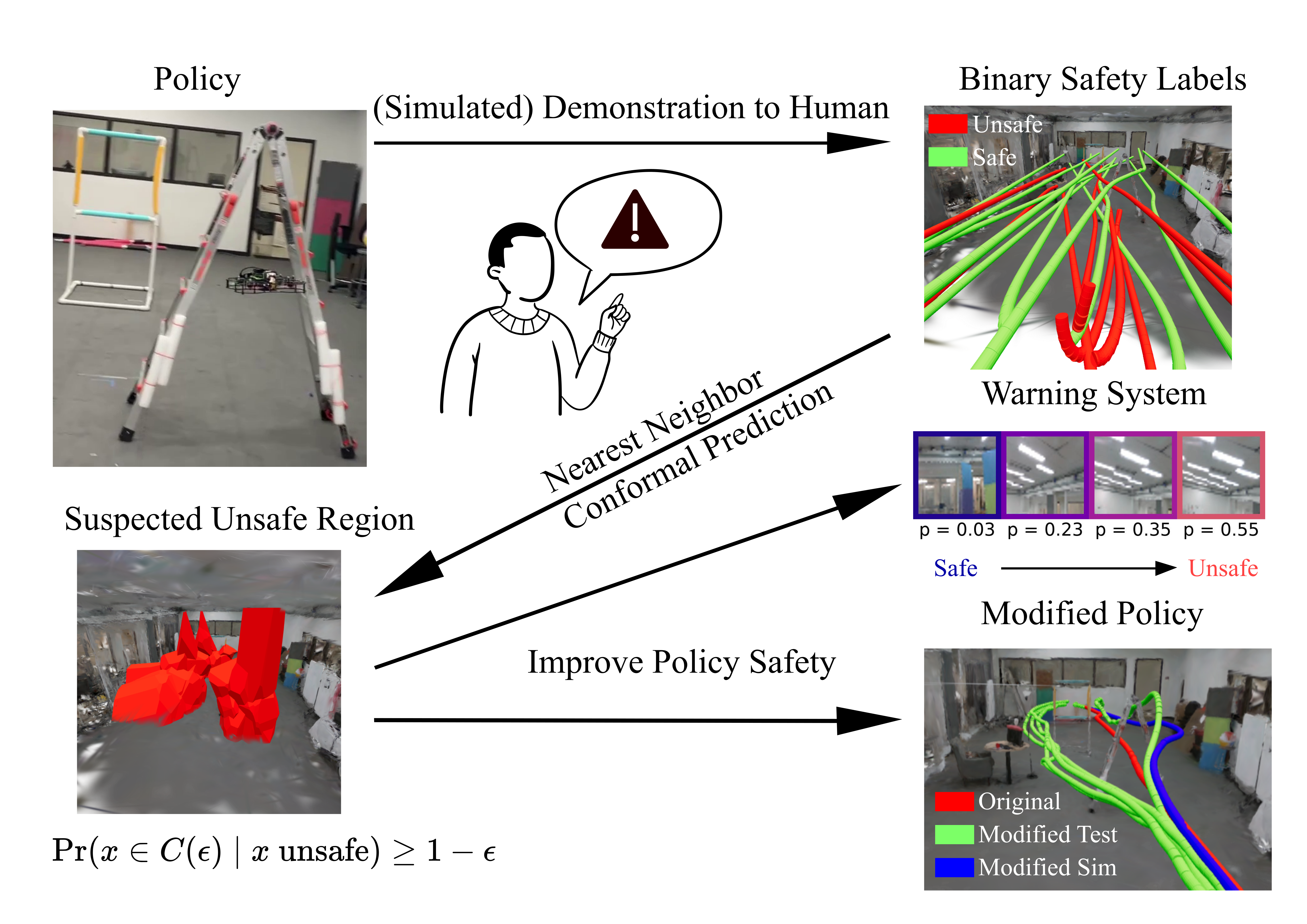
Figure 1: Overview of our approach to learning robot safety from sparse human feedback. Given a robot policy, we repeatedly demonstrate it to a human, possibly in simulation, and have them terminate any trajectories which they deem unsafe. Using these binary labels, we apply conformal prediction to calibrate a nearest neighbor classifier and determine a suspected unsafe region $C(\epsilon)$ containing at least $1-\epsilon$ of states that would be deemed unsafe by the human. Using $C(\epsilon)$, we can improve the original policy’s safety via an auxiliary warning system or a backup safety controller. The graphics show experiment results wherein we use human feedback to (i) develop a warning system for a visuomotor quadcopter policy and (ii) increase the safety of a quadcopter model predictive controller.

In any case, there may only be a few instances of policy failure, either due to limited data overall or because policy failure is rare. To be sample-efficient, we parametrize the region of unsafe states using a variant of nearest neighbor classification (as opposed to more data-hungry machine learning methods). Furthermore, we present novel theory showing how we can, even without withholding data, apply the statistical procedure of conformal prediction to calibrate this classifier. We select the classifier threshold to ensure a user-specified fraction $1-\epsilon$ of future unsafe states will get correctly flagged. These results apply without assuming a distribution over unsafe states, with a limited number of unsafe samples, and regardless of classifier quality. From a geometric perspective, the region suspected of being unsafe, termed the suspected unsafe sublevel (SUS) region $C(\epsilon)$, contains those states falling below the calibrated classification threshold.

Beyond sample efficiency and theoretical guarantees, our approach benefits from simplicity and interpretability. Besides the fraction $1-\epsilon$, the user simply provides a pairwise measure of dissimilarity between states (e.g., Euclidean distance), and the theoretical guarantees apply regardless of this chosen measure. The approach is interpretable as the SUS region $C(\epsilon)$ often adopts a geometrically convenient form, such as a union of polyhedra. Thus, it can be visualized in low dimensions or used to impose avoidance constraints on the original policy.

We discuss two approaches for using the obtained SUS region to improve policy safety: (i) as an auxiliary warning system, and (ii) for policy modification by avoiding the SUS region. The warning system simply alerts the user if the policy reaches the SUS region. Because of the conformal calibration it achieves a guaranteed miss rate, failing to alert in at most $\epsilon$ of unsafe policy executions. Beyond hard classification, the warning system can also act as a runtime safety monitor, providing an interpretable and calibrated scalar measure of safety throughout policy execution. The policy may also be modified to avoid entering the SUS region. As one such implementation, we consider modifying a model predictive control (MPC) policy to switch to a backup safety mode which steers to historical safe data when the MPC planned states are predicted to enter the SUS region.

We demonstrate our approach for learning a warning system and policy modification in simulated examples where a quadcopter must navigate while avoiding a priori unknown obstacles. We also use our approach to learn a warning system from human video labeling of a visuomotor quadcopter policy, fitting the nearest neighbor classifier in a learned latent space of images. Using it, we can preemptively alert when the visuomotor policy will fail to pass through a designated gate. We also test our policy modification approach in hardware experiments where a quadcopter policy is modified to more cautiously navigate in a test environment using human feedback obtained in a Gaussian Splat simulator. We provide an overview of our approach and highlight some experimental results in Figure 1.

In summary, our primary contributions are,

• We present novel theory to perform conformal prediction with nearest neighbor classification in closed-form without holding out data.

• From human feedback, we obtain a calibrated warning system guaranteed to flag a user-specified fraction of future policy errors.

• We can improve the robot policy by using a backup safety mode which is triggered upon a warning system alert.

II Literature Review

We first discuss related works in the robotics literature for data-driven learning of robot safety and then turn to related applications of conformal prediction in robotics.

II-A Learning Robot Safety

Learning about robot safety from data has been tackled in a variety of ways. We categorize these approaches based on how they collect data: from expert demonstration, with binary stop feedback, or via expert assistance.

II-A1 Learning Constraints from Expert Demonstrations

Several approaches have focused on learning safety constraints from an expert demonstrator that acts optimally while respecting the unknown safety constraints. Assuming a nominal reward function and demonstrator noise model, [1] proposes to sequentially infer the most likely constraints restricting motion, referred to as maximum likelihood constraint inference. This approach is extended in [2, 3, 4] to continuous state spaces, stochastic dynamics, and to avoid explicitly searching over a discrete set of potential constraints.

An alternative is to find states guaranteed to be safe/unsafe as implied by the optimal demonstrations. [5] solves a mixed integer feasibility program over cells in the state space, requiring optimal demonstrations to hit only safe cells and lower cost trajectories to hit an unsafe cell. [6] instead solves this program over parameters defining the constraints, and [7] avoids sampling lower cost trajectories using the Karush-Kuhn-Tucker (KKT) conditions. [8] instead uses the KKT conditions to fit a Gaussian process model of the unknown constraint.

Our approach contrasts with methods learning from safe, optimal demonstration data in two key respects. Firstly, we do not assume access to a known reward function nor to demonstrated trajectories which are optimal while respecting the unknown constraints. Secondly, using conformal prediction, our recovered constraint set provides guaranteed coverage of the unsafe set without parametric/distributional assumptions.

II-A2 Learning Safety from Binary Feedback

As in our work, several others have considered learning safety from a binary feedback function that only indicates when a state is unsafe. [9] and [10] repeatedly query this function during reinforcement learning training to simultaneously fit a safety-constrained policy and a safety critic which predicts future failure probability. [11] also considers iteratively updating a safety constraint function using binary feedback, adopting a Bayesian framework and incorporating this learned function as a penalty in policy optimization. These works consider multiple iterations of (typically simulated) environment interaction to incrementally improve policy safety. In contrast, we use offline batch data, with few unsafe samples, to make a given policy significantly safer in a single iteration.

More similar to our work is [12] which learns a safety critic from offline trajectory data and then learns a recovery policy to minimize the critic’s predicted risk. Instead of learning a safety critic, [13] queries the binary safety function online within a look-ahead MPC framework. Since we assume safety is either unknown or expensive to evaluate, we instead learn the SUS region and use the associated warning system as a proxy for binary safety feedback.

II-A3 Learning Safety from Human Interaction

Several works have considered learning safety through interaction with an expert. [14] assumes an expert intervenes to steer the robot back to safety and learns a safety score model from when the expert chooses to intervene and their actions. [15] uses human directional corrections to learn a parameterized but unknown safety constraint. In the context of shared human-robot control, [16] learns a motion assistance system to correct human inputs to better abide an unknown constraint. [17] has the human push the robot to outline the boundary of the safe set and incrementally learns a polyhedral approximation. While we consider using human feedback for learning safety, we only require the human to terminate trajectories when they become unsafe, a simpler task than direct control or intervention.

II-B Conformal Prediction in Robotics

Conformal prediction has gained popularity in robotics as a distribution-free method to improve robot safety. We focus on two related applications where it has been used: for anomaly detection and collision avoidance.

II-B1 Conformal Prediction for Anomaly Detection

Anomaly detectors seek to flag instances unlikely to be drawn from the same distribution as a provided dataset. Conformal prediction is used to calibrate the rate of false alarms without imposing distributional assumptions. Early examples are [18, 19, 20] which apply the full conformal prediction variant to nearest neighbor classification and kernel density estimation to detect anomalous trajectories. Our work also uses full conformal prediction with nearest neighbor classification, but over single states rather than trajectories, and we prove that it can be done in closed-form.

More recently, [21] used the split conformal prediction variant to detect anomalous pedestrian behavior by calibrating the alert threshold for an ensemble of neural network trajectory forecast models. [22] detects anomalous images causing a perception failure by training an autoencoder to reconstruct the training images. When the reconstruction error exceeds a threshold selected via split conformal prediction, they trigger a fallback controller to steer to a designated recovery set. This approach is similar to ours for policy modification, and we use safe historical data to define the recovery set.

While the aforementioned works used conformal prediction to bound the false alarm rate, [23] uses split conformal prediction with unsafe samples to bound the miss rate (i.e., the probability of failing to alarm in unsafe cases). They assume a predefined scalar function reflecting safety, while we directly learn safety from observed safe and unsafe states.

II-B2 Conformal Prediction for Collision Avoidance

Conformal prediction has also been widely used to improve robot collision avoidance by accounting for prediction and environment uncertainty. [24, 25] use split conformal prediction to produce uncertainty sets for predicted pedestrian motion which their robot policy then avoids. To avoid using a union bound, [26] instead finds a simultaneous set over the prediction horizon and [27] provides a modification to ensure recursive MPC feasiblity. In contrast with these works, we use full conformal prediction to avoid reserving data for calibration and focus on learning policy safety directly without pre-trained models.

Instead of using previous trajectories, [28] adaptively learns the forecasting error from previous errors observed within the given trajectory. This violates exchangeability and so they use a modified conformal prediction method for time-series [29]. [30] presents a similar approach but uses Hamilton-Jacobi reachability to transform from confidence sets over actions to states. In our work, by extracting the first unsafe state encountered during policy execution, we can yield a formal guarantee on the multi-timestep error probability without relying on modified conformal prediction methods for time-series [29, 31, 32] which provide somewhat weaker guarantees.

III Overview of Conformal Prediction

Conformal prediction [33, 34] starts with the question: Given $N+1$ random variables (scores) $s_{1},...,s_{N},s_{N+1}$ which are exchangeable, equally likely under permutation, what can be said about the value of $s_{N+1}$ relative to $s_{1},...,s_{N}$? If we assume no ties, the answer is that

$$\Pr(s_{N+1}\leq s_{(k)})=\frac{k}{N+1}$$ (1)

since $s_{N+1}$ is equally likely to achieve any rank in a sorting of $s_{1},...,s_{N+1}$. Here $s_{(k)}$ refers to the $k$’th order statistic of $s_{1},...,s_{N}$ (the $k$’th smallest value). If ties may occur, then the above equality is relaxed to $\geq$.

Using this result, we can produce a probabilistic upper bound on $s_{N+1}$ using $s_{1},...,s_{N}$. Since $s_{1},...,s_{N}$ are random, the bound is random and so the user specifies with what probability the bound should hold: $1-\epsilon$. We call $1-\epsilon$ the coverage probability and $\epsilon$ the miscoverage probability. Taking

$$k(\epsilon)=\lceil(N+1)(1-\epsilon)\rceil,$$ (2)

$$\Pr(s_{N+1}\leq s_{(k)})\geq 1-\epsilon$$ (3)

where this holds for any distribution. Provided exchangeability holds, the scores may be obtained by applying any function to the original data. In this case, bounds on $s_{N+1}$ correspond to confidence sets for new data.

In split (or inductive) conformal prediction [35], the scores are computed by applying a fixed function $s_{i}=s(X_{i},Y_{i})$ to each IID datum $(X_{i},Y_{i})$. This approach is used in much of the recent robotics literature which requires held-out calibration data to compute $s_{1},...,s_{N}$. While Equation 3 holds in expectation (over repeated draws of the calibration set), for one calibration set the coverage is known (assuming continuous IID scores) to follow a Beta distribution [36].

In contrast, full (or transductive) conformal prediction [37], used in this work, achieves exchangeability by swapping data ordering. The score function can now depend on several inputs simultaneously as long as it is symmetric. Given IID points $x_{1},...,x_{N}$ and a candidate point $x$, the score function $s(D;x)$ measures the dissimilarity (as user-defined) between $x$ and the dataset $D$ of the remaining $N$ points (lower scores being more similar). The scores are obtained by swapping $x$ with the different $x_{i}$ i.e., looking at each of the leave-one-out scores:

$$s_{1}^{x}=s(x,x_{2},...,x_{N};x_{1}),s_{2}^{x}=s(x_{1},x,x_{3},...,x_{N};x_{2}),...,$$ (4)

$$s_{N}^{x}=s(x_{1},x_{2},...,x_{N-1},x;x_{N}),s_{N+1}^{x}=s(x_{1},x_{2},..,x_{N};x)$$

The corresponding confidence set for $x$ is defined by

$$C(\epsilon)=\{x\mid s_{N+1}^{x}\leq s_{(k)}^{x}\}$$ (5)

again using $k(\epsilon)$ as in Eq. 2. Then, if $x$ is exchangeable, [33],

$$\Pr(x\in C(\epsilon))\geq 1-\epsilon.$$ (6)

Full conformal prediction allows for more flexible score functions and does not require separate calibration data. However, the dependence on $x$ in both sides of Equation 5 often makes $C(\epsilon)$ intractable to compute in closed-form (although circumventions exist [38, 39, 40]). We avoid such complexity by using the nearest neighbor distance as the score function. In this case, we prove that we can pre-compute a single threshold $r$ defining $C(\epsilon)$. At inference, we need only check $s_{N+1}^{x}\leq r$ to check whether $x\in C(\epsilon)$. Furthermore, we can easily geometrically describe and visualize $C(\epsilon)$.

IV Problem Setting and Approach Overview

Let $\mathcal{X}$ denote the state space of the robot system and $\mathcal{U}$ refer to the associated action (control input) space. We assume a Markovian, time-invariant system evolving via transition dynamics $\mathcal{T}:\mathcal{X}\times\mathcal{U}\rightarrow\mathcal{X}$ and with starting state distribution $\mathcal{D}$. Let $\mathcal{A}\subset\mathcal{X}$ be the true, unknown subset of states which are unsafe. We assume that $\mathcal{A}$ is time-invariant.

We are given an original closed-loop policy $\pi:\mathcal{X}\rightarrow\mathcal{U}$ mapping from state to action. When executing $\pi$, we assume it is terminated when

• Reaching a set $\mathcal{G}\subset\mathcal{X}$ of goal states.

• First reaching the unsafe set $\mathcal{A}$.

• Neither of the first two conditions have occurred within $T_{max}$ execution steps (a time-out condition).

We make no assumptions about the policy $\pi$, it may be feedback or model predictive control, obtained via imitation or reinforcement learning, and may be deterministic or stochastic.

Given policy $\pi$, we refer to a trajectory rollout $\tau$ of $\pi$ as a closed-loop execution of $\pi$. We obtain $\tau$ by initializing $x_{0}\sim\mathcal{D}$ and then repeatedly execute action $u_{t}\sim\pi(x_{t})$ and update the state $x_{t+1}\sim\mathcal{T}(x_{t},u_{t})$ until termination. We write $\tau=(x_{0},x_{1},...,x_{T})$. In general, trajectories may differ in length so let $\tau(-1)=x_{T}$ denote the last state before termination. By definition $\tau(-1)\in\mathcal{A}$ if and only if $\tau$ is unsafe.

We first collect safety data by repeatedly demonstrating $\pi$ $P$ times to a human to obtain trajectory dataset $D=\{\tau_{1},\tau_{2},...,\tau_{P}\}$. In this demonstration phase, the observer is assumed to stop the trajectory whenever it reaches $\mathcal{A}$. Stopped trajectories are declared unsafe and otherwise declared safe.

In terminating unsafe trajectories, the labeler can act preemptively and the SUS region will reflect their level of caution. For instance, instead of terminating upon collision, trajectories may be terminated if the robot’s motion makes collision seem imminent. With historical or simulation data preemptive labeling can also be done retroactively, simply marking as unsafe the state recorded several timesteps before failure.

Let $D_{A}\subset D$ store the $N$ unsafe trajectories collected and $D_{\overline{A}}\subset D$ store the $P-N$ safe trajectories. Although we assume $N>0$, our approach provides the same form of safety guarantees regardless of the size of $N$. In each of the $N$ unsafe trajectories, we extract the final state (i.e., the first unsafe state flagged by the observer), termed the error state: $E=\{e_{1}=\tau_{1}(-1),...,e_{N}=\tau_{N}(-1)\}$.

V Nearest Neighbor Conformal Prediction

V-A Main Results

In this section, we describe how we use full (transductive) conformal prediction applied to the collected error states $E$ to identify the SUS region $C(\epsilon)$ that in expectation contains at least a $1-\epsilon$ fraction of error states $e\in\mathcal{A}$ that would be reached in future executions of $\pi$. $C(\epsilon)$ contains states whose nearest neighbor in $E$ falls below a distance threshold $r$ i.e., in the sublevel set of the nearest neighbor classifier fit using $E$. We thus term $C(\epsilon)$ the suspected unsafe sublevel (SUS) region. We show how to apply full conformal prediction to select $r$ guaranteeing $1-\epsilon$ coverage without requiring a separate hold-out set for calibration. Since we may often have just a few unsafe data points, the ability to simultaneously use them for classification and calibration is critical.

To use full conformal prediction, we define a nearest neighbor score function:

$$s(D;x):=\min_{x^{\prime}\in D}d(x^{\prime},x)$$ (7)

where $d(x^{\prime},x)$ is any pairwise measure of dissimilarity between two states $x$ and $x^{\prime}$ (decreasing as $x$ and $x^{\prime}$ get increasingly similar). Our analysis guarantees a coverage at least $1-\epsilon$ regardless of what measure is supplied. Furthermore, we impose no assumptions on $d$, it need not be a formal kernel/distance, can be negative, and even asymmetric. That said, certain choices may be more efficient at discriminating safety, yielding a smaller SUS region and fewer false alarms.

Typically in full conformal prediction, given $x_{1},...,x_{N}$ and candidate $x$, we find scores by swapping $x$ with each $x_{i}$ (Eq. 4) and then check if $x$ satisfies the condition to be in $C(\epsilon)$ (Eq. 5). In Theorem V.1, we show that with the nearest neighbor score we can perform full conformal prediction in closed-form (without needing to swap online) and can precompute a threshold $r$ defining $C(\epsilon)$. We defer the proof for this and subsequent theorems in this section to the Appendix.

Theorem V.1 (Closed-Form Conformal Prediction).

Let $D=\{x_{1},...,x_{N}\}$ be states drawn IID from any, possibly unknown, distribution $F$ and suppose we are given a miscoverage rate $\epsilon$. Let $\alpha_{1},...,\alpha_{N}$ be the intra-data nearest neighbor values

$$\alpha_{i}=\min_{x^{\prime}\in D,x^{\prime}\neq x_{i}}d(x^{\prime},x_{i})$$ (8)

and let $k=k(\epsilon)\leq N$ (Eq. 2). Using $r=\alpha_{(k)}$ to form

$$C(\epsilon)=\{x\mid s(D;x)\leq r\}$$ (9)

satisfies for new states $x_{N+1}\sim F$

$$\Pr[x_{N+1}\in C(\epsilon)]\geq 1-\epsilon.$$ (10)

Since Theorem V.1 requires $k(\epsilon)\leq N$, the number of samples imposes a minimum level of miscoverage that may be guaranteed $\epsilon\geq 1/(N+1)$.

In Theorem V.1, we showed that we could offline find a cutoff $r$ such that $C(\epsilon)=\{x\mid s(D;x)\leq r\}$. Since $s(D;x)=\min_{x^{\prime}\in D}d(x^{\prime},x)$, we can equivalently describe $C(\epsilon)$ as a union of sublevel sets of $d$ about each datum $x_{i}$. We formalize this result in Theorem V.2.

Theorem V.2 (Geometric Coverage Set).

We may equivalently describe $C(\epsilon)$ from Theorem V.1 (using the cutoff value $r$) as

$$C(\epsilon)=\cup_{i=1}^{N}C_{i}$$ (11a)

$$C_{i}=\{x\mid d(x_{i},x)\leq r\}.$$ (11b)

With this representation, we can geometrically describe $C(\epsilon)$ for many standard choices of $d$. For instance, with Euclidean distance $d(x,y)=||x-y||_{2}$ we obtain a union of closed balls where each ball $C_{i}$ has shared radius $r$ and is centered at one of the states $x_{i}$. Figure 2 (top) provides an example visualizing the geometry of $C(\epsilon)$ when using Euclidean distance.

Figure 2: Visualizing the geometry of the unsafe-only (Eq. 7) and unsafe-safe (Eq. 14) conformal covering set $C(\epsilon)$. We sample $N=30$ unsafe points (shown in red) and $M=100$ safe points (shown in blue) and request miscoverage of $\epsilon=0.1$. In the top subfigure, we plot $C(\epsilon)$ for the unsafe-only case using Euclidean distance. In the bottom subfigure, we use the difference of squared Euclidean distance for the unsafe-safe case (Eq. 18) resulting in a union of polyhedra (see subsection V-B).

While Theorem V.1 ensures $C(\epsilon)$ achieves at least $1-\epsilon$ coverage, we can provide a theoretical upper bound on the coverage, distinguishing between the case of a symmetric versus asymmetric choice of $d$. The upper bound holds when the probability of having distance ties is $0$. Informally, this holds in the general setting of a continuous state space and for non-trivial $d$ (e.g., avoiding $d(x,y)=0$).

Theorem V.3 (Overcoverage Bound: Symmetric Case).

Consider a symmetric pairwise function $d$ which satisfies for samples $x_{1},x_{2},...,x_{N},x_{N+1}\sim F$, the associated pairwise distances $\{d(x_{i},x_{j})\}_{i<j}$ feature no repeated values with probability 1. Then, $C(\epsilon)$ as constructed in Theorem V.1 satisfies:

$$\Pr[x_{N+1}\in C(\epsilon)]\leq 1-\epsilon+2/(N+1).$$ (12)

In conformal prediction without ties, the overcoverage is bounded by $1/(N+1)$, but with a symmetric $d$ ties occur when two points are each other’s nearest neighbors so we get the slightly weaker $2/(N+1)$.

We illustrate the validity of Theorem V.1 and Theorem V.3 in Figure 3 (top) which shows that in repeated generations of $C(\epsilon)$ the coverage fluctuates but indeed has the average coverage between $1-\epsilon$ and $1-\epsilon+2/(N+1)$. Besides reducing the $2/(N+1)$ theoretical overcoverage gap, increasing $N$ should also decrease the coverage fluctuation across repetitions. 

While Theorem V.3 assumed $d$ was symmetric, we provide a similar result in Theorem V.4 bounding the overcoverage for an asymmetric $d$. This result applies in the unsafe-safe nearest neighbor approach we develop in subsection V-B and Figure 3 (bottom) illustrates the validity of the asymmetric overcoverage bound.

Theorem V.4 (Overcoverage Bound: Asymmetric Case).

Consider an asymmetric pairwise function $d$ such that for samples $x_{1},x_{2},...,x_{N},x_{N+1}\sim F$, the associated pairwise distances $\{d(x_{i},x_{j})\}$ feature no repeated values with probability 1. Then, $C(\epsilon)$ as constructed in Theorem V.1 satisfies:

$$\Pr[x_{N+1}\in C(\epsilon)]\leq 1-\epsilon+1/(N+1)+1/N.$$ (13)

Figure 3: Empirical verification of the theoretical coverage guarantees. For both the unsafe-only and unsafe-safe cases, we construct $C(\epsilon)$ $1000$ times with fresh data (using the same setup of Figure 2) and evaluate coverage using $1000$ new unsafe test points. We plot a histogram of the coverage over these repetitions and plot the the average coverage as a green dashed line. The average coverage lies between the theoretical lower (Theorem V.1) and upper bounds (Theorem V.3 for the unsafe-only case and Theorem V.4 for the unsafe-safe case), shown respectively as red and blue dashed lines.

V-B Unsafe-Safe Nearest Neighbor Extension

Until now we have used samples $D_{F}=\{x_{1},...,x_{N}\}$ from a single distribution $F$, in our case the policy error distribution, to produce $C(\epsilon)$. However, for $C(\epsilon)$ to better distinguish safe from unsafe data, we extend our approach to also leverage data from safe trajectories. Let $D_{G}=\{y_{1},...,y_{M}\}$ be points generated under the safe distribution $G$. Our hope is that by also using this safe data in nearest neighbor conformal prediction, $C(\epsilon)$ will still contain $1-\epsilon$ of future unsafe points drawn from $F$ but fewer safe points drawn from $G$.

To incorporate the safe data, we use the difference between the nearest neighbor distances for the unsafe and safe data,

$$s(x)=\min_{x^{\prime}\in D_{F}}d(x^{\prime},x)-\min_{y^{\prime}\in D_{G}}d(y^{\prime},x).$$ (14)

With this new unsafe-safe score, it remains to show how we can apply our conformal prediction results to calibrate it i.e., obtain a cutoff $r$ guaranteeing a miss rate of at most $\epsilon$: $\Pr(s(x)>r\mid x\sim F)\leq\epsilon$. To do so, we exploit that the pairwise function $d$ may be asymmetric in the nearest neighbor procedure described in Theorem V.1. Define

$$\tilde{d}(x^{\prime},x)=d(x^{\prime},x)-\min_{y^{\prime}\in D_{G}}d(y^{\prime},x)$$ (15)

so that

$$s(D_{F};x)=\min_{x^{\prime}\in D_{F}}d(x^{\prime},x)-\min_{y^{\prime}\in D_{G}}d(y^{\prime},x)=$$ (16a)

$$\min_{x^{\prime}\in D_{F}}[d(x^{\prime},x)-\min_{y^{\prime}\in D_{G}}d(y^{\prime},x)]=$$ (16b)

$$\min_{x^{\prime}\in D_{F}}[\tilde{d}(x^{\prime},x)].$$ (16c)

We have thus recast this as a nearest neighbor score with an asymmetric measure $\tilde{d}$. With this perspective, we may now calibrate using the samples from $D_{F}$, treating $s$ as simply a more complicated score. Therefore, (using Theorem V.1) we can calibrate in closed-form by computing

$$\alpha_{i}=\min_{x^{\prime}\in D_{F},x^{\prime}\neq x_{i}}\tilde{d}(x^{\prime},x_{i})=$$ (17a)

$$\min_{x^{\prime}\in D_{F},x^{\prime}\neq x_{i}}d(x^{\prime},x_{i})-\min_{y^{\prime}\in D_{G}}d(y^{\prime},x_{i})$$ (17b)

for $i=1,2,...,N$ and obtaining $r=\alpha_{(k)}$ as before.

A notable special case is squared Euclidean distance:

$$s(D_{F};x)=\min_{x^{\prime}\in D_{F}}||x^{\prime}-x||^{2}-\min_{y^{\prime}\in D_{G}}||y^{\prime}-y||^{2}$$ (18)

which we motivate in the Appendix based on a connection with Gaussian kernel density estimation and likelihood ratio testing. In this case, the resulting conformal set $s(D_{F};x)\leq r$ again has convenient geometry. Applying Theorem V.2 to the asymmetric distance Eq. 15, we obtain $C(\epsilon)=\cup_{i=1}^{N}C_{i}$ where

$$C_{i}=\{x\mid\tilde{d}(x_{i},x)\leq r\}=$$ (19a)

$$\{x\mid d(x_{i},x)-\min_{y^{\prime}\in D_{G}}d(y^{\prime},x)\leq r\}=$$ (19b)

$$\{x\mid d(x_{i},x)-d(y_{j},x)\leq r\ \forall j=1:M\}.$$ (19c)

In the special case of squared Euclidean distance, we get

$$||x_{i}-x||^{2}-||y_{j}-x||^{2}\leq r\ \forall j=1:M$$ (20)

yielding $M$ half-space constraints $a_{ij}^{T}x\leq b_{ij}$ where $a_{ij}=y_{j}-x_{i}$ and $b_{ij}=\frac{r+||y_{j}||^{2}-||x_{i}||^{2}}{2}$. $C_{i}$ consists of an intersection of half-space constraints i.e., a polyhedron. Thus, $C(\epsilon)$ is a union of $N$ polyhedra each with $M$ constraints.

Fig. 2 (bottom) shows the geometry of $C(\epsilon)$ constructed using the unsafe-safe score (Eq. 14). Qualitatively $C(\epsilon)$ constructed with the unsafe-safe score bleeds over less into the region of safe points, and in our later warning system experiments (Section VII) we show this results in fewer false alarms.

V-C Probabilistic Interpretation

Beyond hard classification of whether a state is considered unsafe, we can use the nearest neighbor conformal approach to provide a probabilistic interpretation of safety, using the conformal prediction $p$-value [33].

Definition V.1 (Conformal $p$-Value).

For state $x$, the $p$-value is the smallest $\epsilon$ for which $x\notin C(\epsilon)$, denoted $\epsilon^{*}$.

This matches the standard definition of $p$-value as the smallest size $\epsilon$ under which a hypothesis test rejects. In this setting, we default to the null hypothesis that $x\sim F$ (i.e., $x$ is like $x_{1},...,x_{N}$) and reject when $x\notin C(\epsilon)$. Intuitively, smaller $\epsilon^{*}$ reflects stronger evidence that $x_{N+1}$ is unlike $x_{1},...,x_{N}$. Hence, for $x_{1},...,x_{N}$ unsafe a larger $\epsilon^{*}\in[0,1]$ indicates $x_{N+1}$ is seemingly less safe. For a given cutoff $\epsilon$ and state $x_{N+1}$ with $p$-value $\epsilon^{*}$, by definition $x_{N+1}\in C(\epsilon)$ if and only if $\epsilon^{*}\geq\epsilon$. Thus, the $p$-values can be viewed as describing the increasing growth of the suspected unsafe region $C(\epsilon)$ as $\epsilon$ is decreased. Figure 4 visualizes how the $p$-value varies throughout space when using the unsafe-only and unsafe-safe nearest neighbor approaches. Qualitatively, lower $p$-values are attained in the safe region when using the unsafe-safe approach suggesting that the unsafe-safe approach is better able to distinguish the safe from unsafe data.

Figure 4: Visualizing the $p$-value associated with $C(\epsilon)$. Using the same setup as in Fig. 2, we vary $\epsilon$ to visualize the $p$-value level sets for the unsafe-only (top) and unsafe-safe (bottom) cases. While both the unsafe-only and unsafe-safe cases provide valid coverage of at least $1-\epsilon$, based on the $p$-value visualizations we qualitatively observe that the unsafe-safe approach better distinguishes the unsafe and safe samples.

V-D Combining with Representation Learning

While the conformal guarantee of $1-\epsilon$ coverage will hold when using any dissimilarity measure $d(x^{\prime},x)$, better choices of $d$ can yield fewer false alarms i.e., declaring a state $x$ unsafe when it is actually safe. Therefore, to reduce false alarms, we can learn more effective $d$, learning features of the original data to better distinguish safe and unsafe data. We first transform to this learned space and then apply the conformal nearest neighbor procedure yielding the score function

$$s(D;x)=\min_{x^{\prime}}d(\phi(x^{\prime}),\phi(x)).$$ (21)

This may be viewed as an alternative choice of $d$ which first applies the learned transformation $\phi$. As long as $\phi$ is not fit using the calibration data i.e., the error states $E$, the nearest neighbor approach still guarantees $1-\epsilon$ coverage.

The problem of representation learning is extremely well-studied. Methods can be unsupervised or supervised, using class labels to better separate class distributions. Classical approaches include principle component analysis (PCA) and its kernelized variant [41, 42], unsupervised, and large margin nearest neighbor (LMNN) [43], supervised. In recent literature, DINO/DINOv2 [44, 45], unsupervised, and CLIP [46], supervised, are notable examples. Even in the big-data regime, these recent methods have shown good performance for images by combining representation learning and nearest neighbor classification. In Section VII, we use representation learning with our nearest neighbor approach to scale to image data and detect unsafe behavior for a visuomotor quadcopter policy.

VI Warning System

Directly applying the theoretical results in Section V, we can augment $\pi$ (the policy under which the human feedback data was collected) with a warning system achieving a guaranteed miss rate i.e., the probability of failing to alert when the human would have alerted is no more than the user-specified $\epsilon$.

Offline, using the $N$ error states $E$ obtained when demonstrating $\pi$, we compute the intra-dataset nearest neighbor distances $\alpha_{1},...,\alpha_{N}$ as in Theorem V.1. In the unsafe-only case with Euclidean distance this may be achieved by constructing a KD tree [47], which can be reused at runtime. For the unsafe-safe extension (subsection V-B), we again compute the intra-dataset nearest neighbor distances for each state in $E$, but subtract the distance to the nearest safe neighbor. Given a user-specified miss rate $\epsilon$, we compute $k(\epsilon)=\lceil(1-\epsilon)(N+1)\rceil$ and obtain cutoff $r=\alpha_{(k)}$.

During policy execution, for each new observed state $x$, we compute the nearest neighbor score $s(D;x)$ and alert if $s(D;x)\leq r$ i.e., the state is in the SUS region $x\in C(\epsilon)$. This alert may be used in a variety of ways, from simply aborting policy execution (e.g., by transitioning a quadcopter to hover), signaling for human takeover, or triggering a fallback to historical safe data (see Section VIII).

Our previous results in Sec. V held for IID data and a single query. At runtime, we repeatedly query the warning system. Nevertheless, the states in $E$ are independent and if the current state is an error state it will be exchangeable with $E$. Thus, our warning system retains the miss rate guarantee in the multi-timestep setting, which we formally show in Theorem VI.1.

Theorem VI.1 (Warning Miss Rate).

Let $\tau$ be a new trajectory generated by executing $\pi$.

$$\Pr(\mbox{$\tau$ yields no alert}\mid\tau\mbox{ reaches $\mathcal{A}$})\leq\epsilon.$$ (22)

Proof.

Since trajectories are terminated upon reaching $\mathcal{A}$, $\tau$ reaches $\mathcal{A}$ if and only if $\tau(-1)\in\mathcal{A}$. $\tau$ yields no alert when $\forall i:\tau(i)\notin C(\epsilon)$. Thus, the left side of Eq. 22 is equivalent to

$$\Pr(\tau(i)\notin C(\epsilon)\ \forall i\mid\tau(-1)\in\mathcal{A}).$$ (23)

No alert at all times implies no alert at the final time hence

$$\Pr(\tau(i)\notin C(\epsilon)\ \forall i\mid\tau(-1)\in\mathcal{A})\leq$$ (24)

$$\Pr(\tau(-1)\notin C(\epsilon)\mid\tau(-1)\in\mathcal{A})$$

By the conformal guarantee,

$$\Pr(\tau(-1)\notin C(\epsilon)\mid\tau(-1)\in\mathcal{A})\leq\epsilon.$$ (25)

∎

As a corollary, we can bound the overall probability $\pi$ becomes unsafe without warning.

Corollary VI.1.1.

With shorthand $\beta\coloneqq\Pr(\tau\mbox{ reaches $\mathcal{A}$})$,

$$\Pr(\tau\mbox{ reaches $\mathcal{A}$ without a warning})\leq\epsilon\beta.$$ (26)

Proof.

The left side equals

$$\Pr(\tau\mbox{ reaches $\mathcal{A}$ without a warning}\mid\tau\mbox{ reaches $\mathcal{A}$})$$

$$*\Pr(\tau\mbox{ reaches $\mathcal{A}$})\leq\epsilon\beta$$ (27)

by Theorem VI.1. ∎

Using Corollary VI.1.1 we can decide what $\epsilon$ to select. We can approximate $\beta\approx\hat{\beta}=N/P$ using the number of unsafe over total rollouts (or via more conservative failure rate bounds [48]). If we want $\Pr(\tau\mbox{ reaches $\mathcal{A}$ without warning})\leq\eta$ for a user-specified $\eta$ we take $\epsilon$ small enough such that $\epsilon\hat{\beta}\leq\eta$. Of course, a drawback is that smaller $\epsilon$ can increase the number of false alarms (i.e., alerting during a safe trajectory).

VII Warning System Experiments

We evaluate the proposed warning system in two simulated quadcopter settings: 1. an MPC policy navigating in an environment with unknown obstacles and 2. a visuomotor policy navigating through a designated gate. While these are simulation experiments, we use the same MPC formulation in the hardware experiments in Section IX and the visuomotor policy receives photorealistic image data rendered from a Gaussian Splatting model trained from the actual room in the hardware experiments.

VII-A Model Predictive Control Example

In this example, we initialize the quadcopter at random starting states and use an MPC policy to steer to a given goal state. The 9-dimensional quadcopter state includes the position $p=(p_{x},p_{y},p_{z})$, Euler angles $\Theta=(\phi,\theta,\psi)$, and linear velocity $v=(\dot{p}_{x},\dot{p}_{y},\dot{p}_{z})$. At each time the policy outputs a 4-dimensional control action consisting of mass-normalized total thrust $F$ and body angular rates $\Omega$: $u=(F,\omega_{x},\omega_{y},\omega_{z})$. To select the action, the MPC policy optimizes an open-loop plan $H$ steps into the future and applies the first resulting action $u_{0}$. We optimize using sequential convex programming (SCP), repeatedly solving a quadratic program (QP) obtained via affine approximation of the dynamics about the previous intermediate solution $(\overline{x},\overline{u})$:

Here $x_{0}$ is fixed to the current state, $x_{g}$ is the goal state, $u_{g}$ is an associated reference action, $\{Q_{t}\}_{t=0:H},\{R_{t}\}_{t=0:H-1}$ are provided positive-definite cost matrices, $A_{t},B_{t},C_{t}$ are found via affine approximation of $x_{t+1}=f(x_{t},u_{t})$ about $(\overline{x}_{t},\overline{u}_{t})$, $F_{u}(t),g_{u}(t)$ specify control constraints, and $F_{x}(t),g_{x}(t)$ specify state constraints. Further details are in the Appendix.

As an illustrative example with a simple definition of safety, we consider that there are position obstacles unknown to the MPC policy and terminate trajectories upon collision. Figure 5 shows example results of fitting the warning system. The top subfigure shows the labeled demonstration trajectories, obtained by repeating policy execution until getting $N=25$ unsafe trajectories. Using error and safe states, we performed unsafe-safe nearest neighbor conformal prediction (Eq. 18) with $\epsilon=0.2$. Figure 5 (middle) shows a 3-dimensional view of $C(\epsilon)$ which actually exists in the full 9-dimensional state space where it is learned.  In Figure 5 (bottom), we show the warning system in action, terminating trajectories reaching $C(\epsilon)$. As the original policy is often unsafe (crashing in $52\%$ of demonstrations), the warning system is necessarily often triggered, and using it reduces collision to $4\%$ (among $50$ test trajectories).

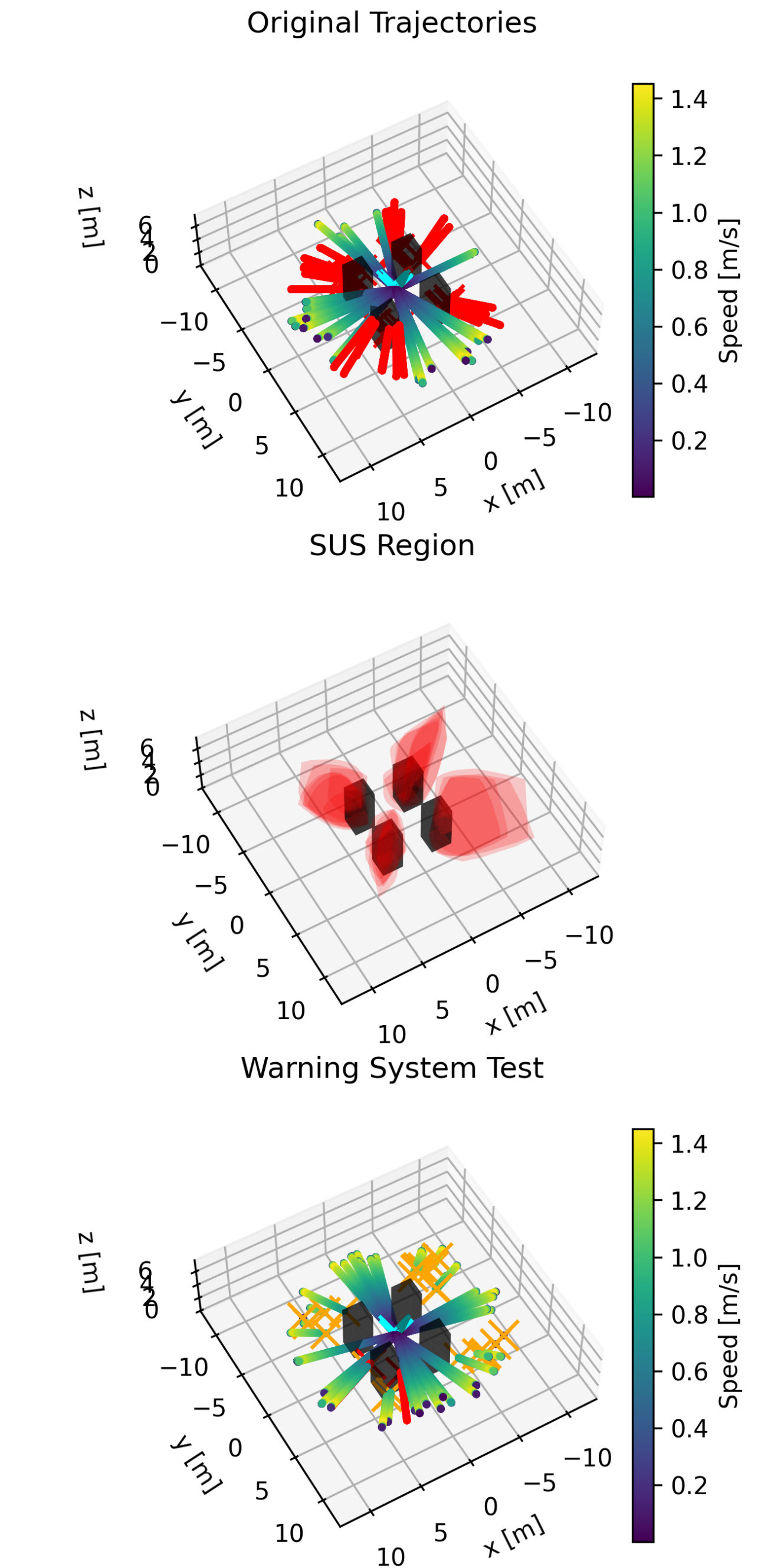
Figure 5: Visualization of our warning system augmenting a quadcopter MPC policy that sometimes collides with unknown obstacles. We specify $\epsilon=0.2$ and use $N=25$ errors for unsafe-safe nearest neighbor conformal prediction. The top subfigure shows the original trajectories, which collide (marked in red) $52\%$ of the time. The middle subfigure shows a 3D visualization of the SUS region $C(\epsilon)$ which actually exists in the 9D state space. The bottom subfigure shows the warning system tested for $50$ new trajectories. States triggering an alert are marked with an orange ‘x.’ Terminating upon alert drops the error rate to $4\%$.

To systematically assess our approach, we fit the warning system over $20$ repetitions, each time collecting $N=25$ unsafe trajectories and a variable number of associated safe trajectories, and evaluate using a test set of $500$ trajectories. For fair comparison, all methods use the same data.

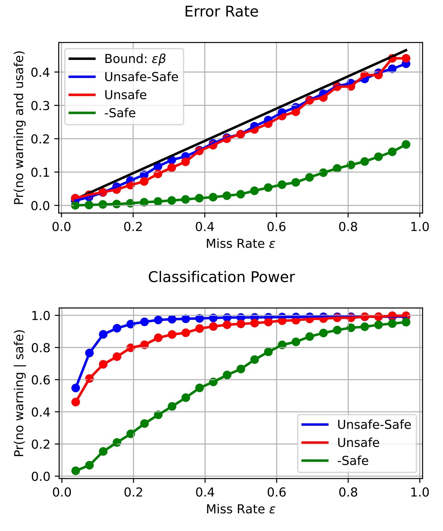
Figure 6: Systematic warning system results for a quadcopter MPC policy generated over $20$ repetitions. In each repetition, we fit our unsafe-safe conformal prediction warning system to new $N=25$ unsafe trajectories and a variable number of associated safe trajectories. We compare against performing conformal prediction using either just the safe or unsafe data. While all methods retain the error rate guarantee (Corollary VI.1.1), as assessed in the top subfigure using a test set of $500$ trajectories, the unsafe-safe approach yields fewer false alarms as shown in the bottom subfigure.

In Figure 6 (top) we verify that for varying $\epsilon\in[\frac{1}{N+1},\frac{N}{N+1}]$, the fraction of test trajectories resulting in error with no alert is $\leq\epsilon\beta$ (Corollary VI.1.1). Besides the unsafe-safe nearest neighbor approach (labeled Unsafe-Safe) we consider as ablations performing the nearest neighbor approach, but only using distance to the nearest unsafe state (labeled Unsafe) or instead flagging if distance to the nearest safe state is too large (labeled -Safe). In all cases Corollary VI.1.1 holds as each approach is nearest neighbor conformal prediction but with a different dissimilarity measure. In Figure 6 (bottom) we plot an ROC-like curve studying classification power as $\epsilon$ varies. The y-axis plots the complement to the false alarm rate i.e., $\Pr(\mbox{no warning}\mid\mbox{safe})$ and should remain high for an effective safety classifier. Across $\epsilon$, the unsafe-safe approach outperforms ablations. Using only safe data performs poorly as new initial conditions can be far from recorded safe trajectories, triggering false alarms.

In Figure 7 we baseline against various machine learning classifiers: a random forest (RF), support vector machine (SVM), and neural network (NN). For each, we also fit with a class balancing variant, weighting the total loss contribution from unsafe and safe samples equally. We fit on the entire data and plot an ‘x’ at the point $x=\Pr(\mbox{no warning}\mid\mbox{ unsafe})$, $y=\Pr(\mbox{no warning}\mid\mbox{ safe})$. Note that these standard techniques do not allow us to control for the miss rate, $\epsilon$, so only one ‘x’ appears per method. To better compare with our nearest neighbor method, we also calibrated each of these baselines using split conformal prediction, reserving $10$ unsafe trajectories from the $25$ for prediction, and plot the ROC-like curves as a function of $\epsilon$ in Fig. 7. Across the $\epsilon$ range our unsafe-safe nearest neighbor conformal approach outperforms all but the random forest with class-balancing which performs similarly. In contrast with this method, we avoid the need for hyperparameter tuning, are able to use all $N=25$ error states (not just a held-out $10$) in conformal prediction yielding better guarantees, and can easily describe the learned SUS region geometrically (which we later exploit for policy modification). Of course, our method will not always outperform these standard and powerful machine learning alternatives. Rather, we propose nearest neighbor conformal prediction as a simple, interpretable, and data-efficient approach that provides theoretical guarantees without hyperparameter tuning or separate calibration data. More baseline implementation details are in the Appendix.

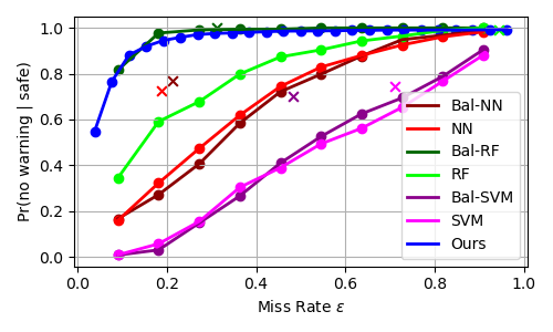
Figure 7: Comparison of our warning system against machine learning baselines. Using the same data as in Fig. 6, we repeatedly fit several machine learning baselines (random forests (RF), neural networks (NN), support vector machines (SVM)) with and without class balancing, shown as ‘x’s on the plot. Furthermore, to control the miss rate $\epsilon$ of these classifiers, we use split conformal prediction which requires holding out calibration data, unlike in our method. Curves show the ROC performance of each method across $\epsilon$. Despite its simplicity, our approach performs similarly to random forest with class-balancing and outperforms all the other methods.

VII-B Visuomotor Quadcopter Policy Example

We also developed our warning system to augment a visuomotor policy tasked with flying a quadcopter through a designated gate. The policy we use is an early version of that developed in [49]. The policy is parameterized as a neural network that takes as input an RGB image and a history of partial state and action information, then outputs as a control action the normalized thrust and body angular rates. To generate training data for the policy, a Gaussian Splat [50, 51] representation of the physical environment is fit using real image data to create a visually realistic simulator. Within this simulator, the policy is trained via behavior cloning to mimic a model-based trajectory optimizer [52] which has privileged information regarding the quadcopter state and quadcopter parameters (mass, thrust coefficient) that are randomized at initialization. For more details, we refer readers to the Appendix and the original work [49].

To fit the warning system, we simulated $200$ trajectories in the Gaussian Splat while randomizing the initial quadcopter state and physical parameters and record the corresponding simulated images. We then watch replayed videos and using a simple user interface, and terminate any trajectories if we were convinced the policy had veered too far and was unlikely to pass through the gate. Using this human feedback, we flagged $45$ of the trajectories as unsafe and stored the $50\times 50\times 3$ downsampled RGB image data for use in the conformal warning system. Downsampled images (in the Gaussian Splat simulator) from an example safe and unsafe trajectory, as labeled by the human, are shown in Figure 8.

Figure 8: Example trajectories rendered in a Gaussian Splat simulator used in fitting the warning system for a visuomotor quadcopter policy. The top row shows downsampled frames from a safe trajectory that successfully passes through the gate and is not stopped by the human. The bottom row shows downsampled frames from an unsafe trajectory that is terminated by the human labeler when it is deemed the quadcopter will not pass through the gate. The final image where the human triggers termination is outlined in red.

Instead of directly using the downsampled images in the nearest neighbor procedure, we reduce the dimension by fitting a representation learning model, reusing the safe trajectories to find a $400$ dimensional latent space. We considered fitting PCA, KPCA, and neural network autoencoder models to this safe data to learn the transformation as well as using a pre-trained CLIP model [46]. We include these comparisons to illustrate our method’s compatibility with a variety of representation learning techniques; the choice of a particular technique is not a key part of our method. We repeatedly ($20$ times) select a random subset of $30$ unsafe and $100$ safe trajectories to fit the warning system and assess performance using the remaining trajectories. We show in Figure 9 (top) the average miss rate (over dataset draws) for varying $\epsilon$ in the warning system. Regardless of transformation, the empirical average falls below the $\epsilon$ value as guaranteed in Theorem VI.1. In Figure 9 (bottom), we show the average empirical estimate of $\Pr(\mbox{no warning}\mid\mbox{safe})$ for each of the warning systems. KPCA and PCA perform comparably, followed by CLIP, and the autoencoder performs poorly (presumably due to limited data). Further details in the Appendix.

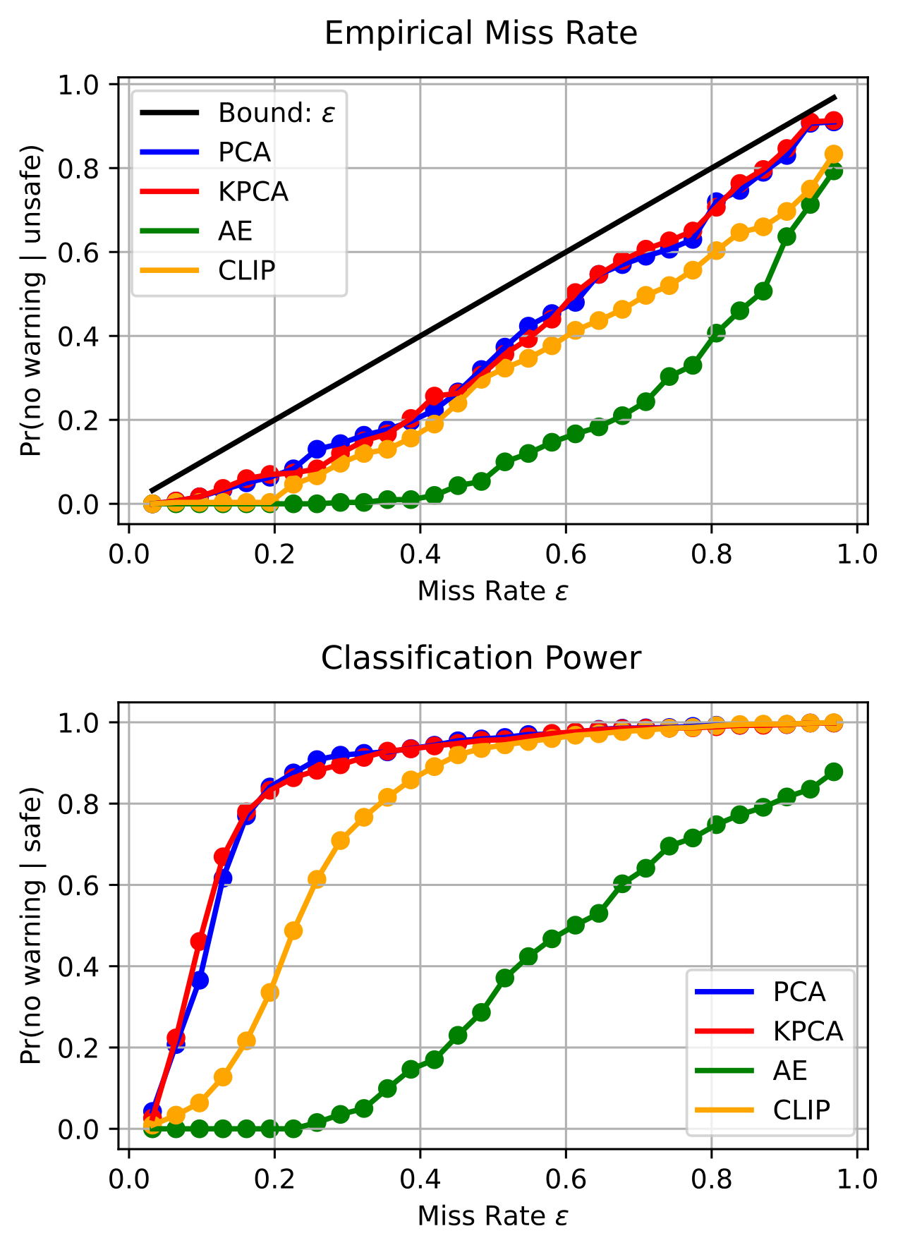
Figure 9: Results for conformal warning systems applied to a visuomotor quadcopter policy with different image representations. The results average across $20$ train-test splits of $200$ trajectories. In each split, $30$ unsafe trajectories and $100$ safe trajectories are used to fit the conformal warning system. The safe trajectories are also used to fit the representation model (except pre-trained CLIP which is fixed). Both PCA and KPCA perform well, but all methods retain Theorem VI.1’s miss rate guarantee.

For one warning system fit, Figure 10 shows downsampled frames (simulated in the Gaussian Splat) from novel test safe and unsafe trajectories. We visualize the associated $p$-value as a border color with warmer colors indicating higher values, i.e., images deemed more unsafe by the warning system. In the (top) safe trajectory the $p$-values remain low while in the (bottom) unsafe trajectory the $p$-values increase as the quadcopter starts flying too high above the gate. Using the $p$-value as a calibrated safety measure, the warning system can thus act as a runtime safety monitor.

Figure 10: Test trajectories in a Gaussian Splat simulator with associated warning system $p$-values. The top row shows a safe trajectory with low $p$-values throughout. The bottom row shows an unsafe trajectory where the $p$-values increase as the quadcopter begins to fly above the gate, not through as desired.

VIII Policy Modification

In this section, we use the warning system (see Section VI) to modify the original policy and improve its safety. Our approach is to avoid the SUS region $C(\epsilon)$, using the warning system to trigger a backup safety controller that steers towards historical safe data. We focus on the MPC setting as we will exploit the ability in MPC to 1. look ahead into the future using the open-loop plan and 2. easily add/enforce constraints by modifying trajectory optimization. In future work, it would be valuable to extend this approach to other settings.

Besides $\pi$, we use an additional backup policy $\pi_{B}$ to track to historical safe trajectories. Offline, we search through the set of safe collected trajectories $D_{\overline{A}}$ and identify the “backup” subset, denoted $D_{B}$, which avoid $C(\epsilon)$. At runtime, we start by using $\pi$, repeatedly solving the optimization in Eq. 28. If any state in the open-loop plan $x_{1:H}$ enters $C(\epsilon)$ i.e., triggers a warning, we record the future alert timestep $t_{w}\in\{1,...,H\}$ and switch to the backup safety mode. When first switching, we identify the nearest safe trajectory $\tau_{B}\in D_{B}$ containing state $x_{B}$ at time $t_{B}$ closest (in Euclidean distance) to the current state $x_{0}$. Our backup policy $\pi_{B}$ will aim to drive the current trajectory towards $\tau_{B}$. At each time while in backup safety mode, we increment $t_{B}=t_{B}+1$ and extract the relevant safe states from $\tau_{B}$ as tracking targets: $x_{B}^{0}=\tau_{B}(t_{B}),...,x_{B}^{H}=\tau_{B}(t_{B}+H)$. $\pi_{B}$ solves a similar optimization to Eq. 28 except instead of a single goal state $x_{g}$, we track the selected backup states $\{x_{B}^{t}\}$, solving the below optimization and applying $u_{0}$:

We release the backup safety mode and return to using $\pi$ if either (i) the current state $x_{0}$ is close to $\tau_{B}$ and at least $t_{w}$ timesteps have elapsed, or (ii) a maximum number of iterations has elapsed. Since we do not track $\tau_{B}$ indefinitely, our approach applies even if the goal region changes run to run, as shown in our hardware experiments.

We impose additional state constraints in Eq. 29 to ensure that $\pi_{B}$ avoids the SUS region $C(\epsilon)$ while steering to the historical safe data. Using the SUS region’s geometry (Theorem V.2) as either a union of balls or polyhedra $\cup_{i=1}^{N}C_{i}$, we treat $C(\epsilon)$ as a set of learned obstacles which we constrain $\pi_{B}$ to avoid. Although more sophisticated methods exist [53, 54, 55, 56], we include these constraints in our SCP implementation by conservatively approximating $C_{i}$ using our previous guess. Focusing on the more powerful unsafe-safe case, we require one of the halfspace constraints defining $C_{i}=\{x\mid A_{i}x\leq b_{i}\}$ to be violated (so that we stay out of the unsafe polytope $C_{i}$): $a_{ij}^{T}x>b_{j}$. For given $C_{i}$, state $x_{t}$, and previous guess state $\overline{x}_{t}$ we select $j^{*}=\arg\max_{j=1:M}d_{ij}$ where $d_{ij}=(a_{ij}^{T}\overline{x}_{t}-b_{ij})/||a_{ij}||_{2}$ is the signed distance of $\overline{x}_{t}$ to the $j$-th hyperplane. Each SCP iteration has $N$ added constraints for each state in the horizon: $A_{x}(t)x_{t}\leq b_{x}(t)$. To improve SCP runtime, we can reduce the number of halfspaces defining each $C_{i}$ by subselecting safe states to use in unsafe-safe conformal prediction or by pruning redundant constraints.

We summarize our approach to policy modification below:

1. Offline, collect a backup dataset $D_{B}$ of safe trajectories which do not enter $C(\epsilon)$.

2. Online, use $\pi$ but switch to the backup safety mode if the look-ahead plan $x_{1:H}$ enters $C(\epsilon)$ (at a timestep $t_{w}$).

3. When first switching to the backup safety mode, find the nearest trajectory $\tau_{B}$ to the current state $x_{0}$ with nearest state $x_{B}\in\tau_{B}$ achieved at time $t_{B}$.

4. While in the backup safety mode, increment $t_{B}$ and apply $\pi_{B}$ to steer to tracking targets $\{x_{B}^{t})\}_{0:H}\in\tau_{B}$. Also, add linear constraints to avoid $C(\epsilon)$, one per $C_{i}$.

5. Release the backup safety mode after a maximum elapsed time or if the current state $x_{0}$ is now close enough to $\tau_{B}$ and the original alert time $t_{w}$ has passed.

A straightforward approach to improving the safety of $\pi$ would be to add constraints to avoid $C(\epsilon)$ at all times and forgo using a backup policy. However, modifying $\pi$ to avoid $C(\epsilon)$ causes a distribution shift over the visited states, violating the IID assumption used to calibrate $C(\epsilon)$, and can still result in high error rates as shown in Section IX. By nominally using $\pi$ and switching to $\pi_{B}$ upon alert, there is no distribution shift until alert. Thus, the warning system remains calibrated, reliably detecting unsafe states in the look-ahead plan. Because we switch to $\pi_{B}$ preemptively using alerts in the look-ahead plan, we can hope there is still time for a well-tuned $\pi_{B}$ to steer to the safe data $\tau_{B}$ before reaching an unsafe state. Implicitly, this requires sufficiently diverse backup trajectories in $D_{B}$ so that $\tau_{B}$ is close enough to reasonably be reached using $\pi_{B}$.

IX Policy Modification Experiments

We perform simulation and hardware experiments to evaluate our approach for policy modification. Our simulation experiments extend Section VII; we now show the modified policy can safely navigate to the goal. For our hardware experiments, we use human video feedback collected with a Gaussian Splat simulator to modify a quadcopter MPC policy to navigate more cautiously in the test environment.

IX-A Simulation Experiments

In Figure 11 (top) we show a demonstration of the modified quadcopter MPC policy for $50$ test runs equipped with our backup safety mode. We use the same data as in Figure 5 to construct the warning system offline with $\epsilon=0.1$ and extract the associated polytopes defining $C(\epsilon)$ to constrain the backup policy $\pi_{B}$.  Modifying the policy reduces the empirical collision rate from $52\%$ to $6\%$. We observe that the backup policy $\pi_{B}$ indeed often succeeds in steering around the unknown obstacles. In Figure 11 (bottom) we compare against an ablation which omits using $\pi_{B}$ and instead directly modifies the base MPC policy $\pi$ to avoid $C(\epsilon)$. As discussed further in Section VIII, modifying $\pi$ violates the calibration of $C(\epsilon)$ and this ablation yields an empirical collision rate of $36\%$.

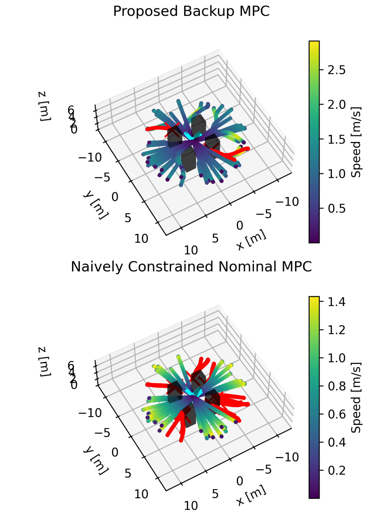
Figure 11: Modifying a nominal MPC policy to avoid $C(\epsilon)$. We specify $\epsilon=0.1$ and use $N=25$ errors with the unsafe-safe nearest neighbor conformal prediction procedure to find $C(\epsilon)$. The top subfigure shows $50$ trajectories executed with our proposed backup MPC that steers to historical safe data while avoiding $C(\epsilon)$. The empirical collision rate is reduced from $52\%$ to $6\%$. The bottom subfigure shows the original policy with constraints added to avoid $C(\epsilon)$. This induces a distribution shift and violates the calibration of $C(\epsilon)$, leading to high collision rates ($36\%$ in this case).

In Figure 12, we provide a systematic comparison of our policy modification approach, labeled “backup MPC,” compared against directly constraining the policy using $C(\epsilon)$, labeled “Naive Const. MPC.” For $20$ repetitions and for $10$ choices of $\epsilon$, We execute $5$ trajectories under each approach (for a total of $100$ per $\epsilon$) and record the resulting policy error rate. As seen also in Figure 11, constraining the original policy does not improve the error rate even as $\epsilon$ is decreased. However, our approach is able to reduce the error rate, in fact, to roughly the warning system error rate of $\epsilon\beta$ (Corollary VI.1.1). This heuristic assumes errors are predominantly caused by failing to alert, which is often reasonable since upon alert we switch to tracking historical safe data and should therefore fail rarely. As with the warning system, the user can use this heuristic and the current error rate estimate $\hat{\beta}$ to choose $\epsilon\leq\eta/\hat{\beta}$ to reduce the modified policy error rate to approximately $\eta$.

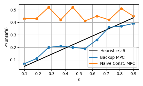
Figure 12: Comparison of our approach for policy modification (labeled backup MPC) against a naive baseline (labeled no track MPC). Over $20$ repetitions, and for different settings of $\epsilon$, we form the modified policy using our and the baseline method and execute $5$ trajectories (for a total of $100$ per $\epsilon$). Due to distribution shift, the baseline which directly constrains the original policy fails to improve policy error. However, our approach is able to improve policy error using $C(\epsilon)$ to define a backup safety mode. In fact, our approach approximately yields the heuristic error rate of $\epsilon\beta$ from Corollary VI.1.1.

IX-B Hardware Experiments

For our hardware experiments, we start with a quadcopter MPC policy that has a minimal level of obstacle avoidance and use human feedback to modify the initial policy to navigate more cautiously around obstacles.  To encode obstacle avoidance into the starting quadcopter MPC, we use a point cloud derived from a Gaussian Splat simulator of the test environment. As described in the Appendix, we do so using unsafe-only nearest neighbor conformal prediction (Section V), approximating the local point cloud as a union of balls then added in MPC constraints. 

Using the Gaussian Splat, the user watches simulated flight trajectories and terminates when the quadcopter is perceived to become unsafe. After acting as human labelers and reviewing $100$ quadcopter trajectories, we flagged $52$ of them as unsafe. These failures were caused by the quadcopter (i) passing too close above the table or trying to go underneath it, (ii) going through the ladder instead of around it, or (iii) going too near/under the gate, and reflect the subjectivity associated with human-determined safety. Figure 13 (left) shows $20$ of these labeled trajectories overlaid on a Gaussian Splat rendering of the test environment, marking safe trajectories in green and unsafe in red. When fitting $C(\epsilon)$ we selected $\epsilon=0.096$ so the heuristic error rate after policy modification would be $\eta=0.05$. We visualize a 3-dimensional view of $C(\epsilon)$ (which actually lives in 9 dimensions) overlaid on the Gaussian Splat in Figure 13 (right). We observe that $C(\epsilon)$ covers the main obstacles (table, lamp, ladder, and gate) flagged by the human. Furthermore, $C(\epsilon)$ reflects the preemptive human labeling as the polyhedra protrude outwards from the front of obstacles.

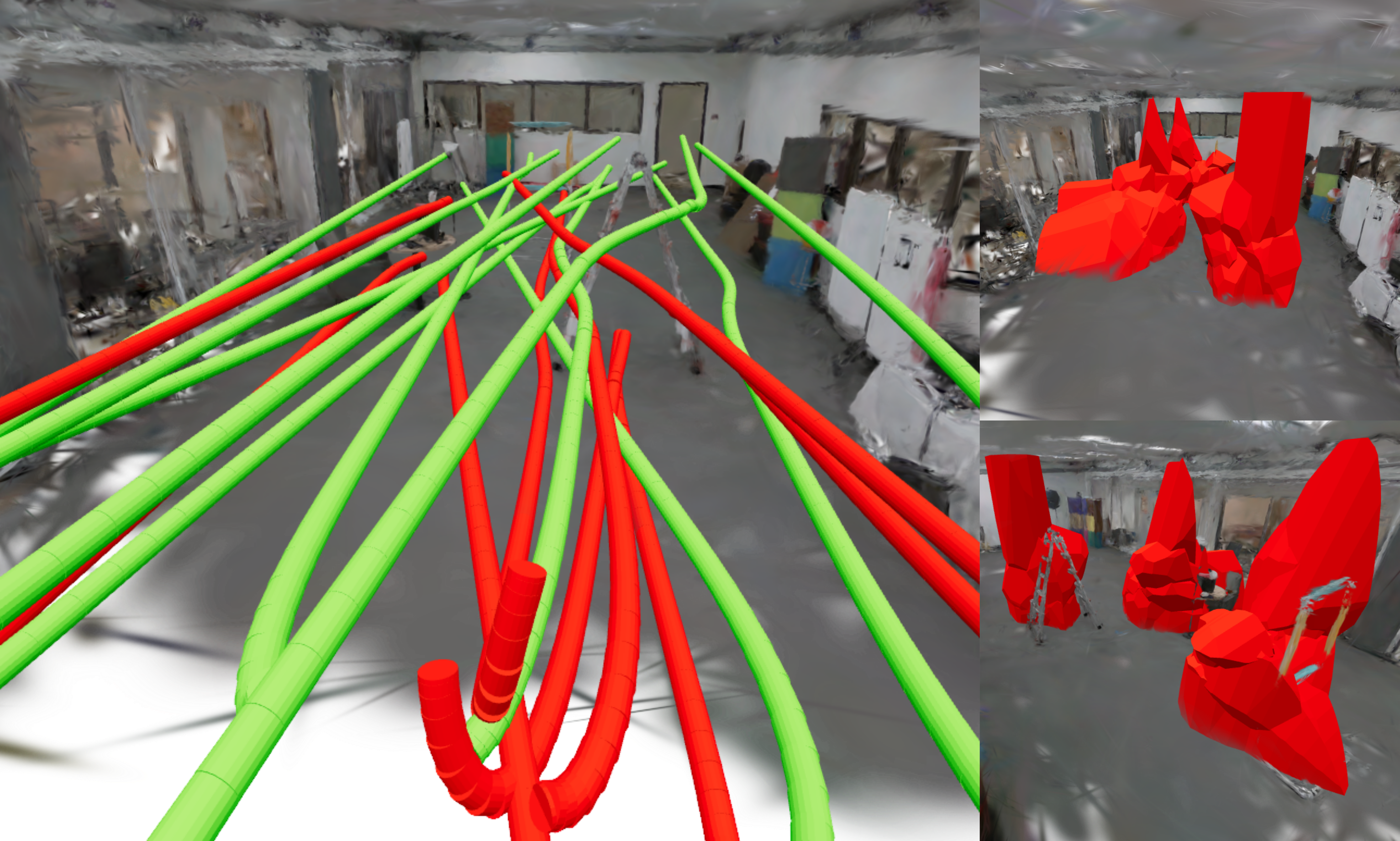
Figure 13: We modify a quadcopter MPC policy to more cautiously navigate around obstacles using human video feedback collected in a Gaussian Splat simulator. The labeled safe and unsafe trajectories are colored green and red respectively in the left subfigure. Using this data, we form the SUS region $C(\epsilon)$ in 9D state space, of which a 3D view is displayed on the right.

Using the approach described in Section VIII, we modify the original MPC policy and perform $30$ flight tests in hardware, performing $5$ trials for $6$ start-goal configurations. We tested starting from two locations (roughly facing the table or the ladder) and targeting three different goals across the room (left, center, or right side). Figure 14 shows a comparison of these flight tests (in green) to simulations using the modified (in blue) or original (in red) policy. The trajectories using the modified policy avoid some of the original unsafe behavior; they go higher above the table (see chair side left goal), do not get stuck near the gate (see chair side center goal), and do not go through the ladder (see ladder side center goal). For each configuration, Figure 14 plots the associated $p$-value over time (see subsection V-C). In simulation, the modified policy (in blue) keeps the $p$-values below the $\epsilon$ threshold while the original policy (in red) exceeds this threshold when nearing the ladder or gate. When the red and blue $p$-value curves fully overlap this reflects that the original policy was deemed safe enough that the backup safety mode was never triggered. The green $p$-value curves associated with the hardware tests, $5$ for each configuration, generally remain below the $\epsilon$ cutoff. However, they occasionally violate (unlike the modified policy in simulation) which can be attributed to the sim-to-real gap e.g., deviation from the modeled dynamics due to low-level flight control, state estimation error etc.  For instance, there is an outlier in ladder side right goal where one of the $5$ hardware tests features a $p$-value spike. Nonetheless, the associated trajectory avoids going under the ladder; it starts moving to the ladder center but then shifts to the right.

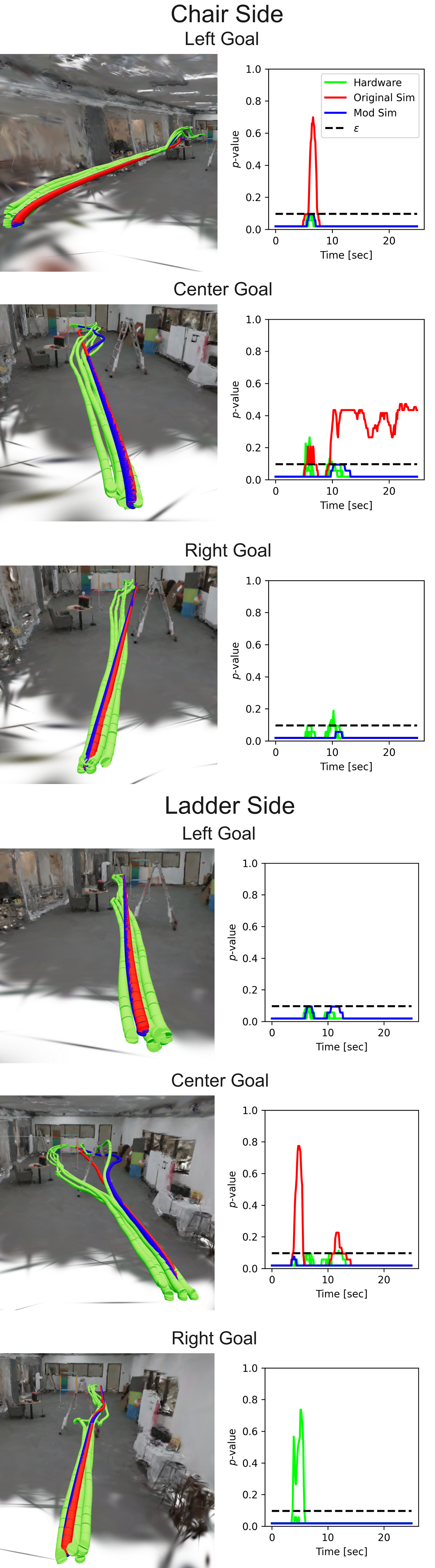
Figure 14: Hardware flight results (in green) using an MPC policy modified via human feedback. We compare to simulated trajectories of the modified (in blue) or original (in red) policy. We performed $5$ tests from $6$ configurations (2 starting locations and 3 goals). The modified policy avoids unsafe behavior flagged by the human (e.g., going under the ladder) and generally keeps $p$-values below the user-specified $\epsilon$ threshold.

X Conclusion

Defining and ensuring safety for a robot policy can be challenging due to environmental uncertainty, policy complexity, or subjective definitions of safety. In this work, we developed an approach for learning about robot safety from human-supplied labels. The human observes a handful of policy executions and terminates the run if the robot reaches an unsafe state (in the human’s subjective sense of safety). Using this data, we fit a nearest neighbor classifier and calibrate it using conformal prediction to correctly flag a user-defined fraction of future errors. We derive novel theory showing we can calibrate without reserving unsafe states (of which there may be few) and provide an equivalent geometric description of the suspected unsafe sublevel (SUS) region. Using this region, we provide a warning system to mimic the safety preferences of the human labeler, up to a user-defined miss rate. More generally, the associated scalar $p$-value can serve as an interpretable safety score for runtime monitoring, giving the probability that a human labeler would raise a flag. We demonstrate the warning system for both simulated quadcopter MPC experiments and for a visuomotor quadcopter policy. Lastly, we use the SUS region for policy modification by adding a backup safety mode which triggers upon warning system alert. We test our policy modification approach in simulated quadcopter MPC experiments and in hardware where we improve navigation using human feedback.

There are several avenues to extend our work and overcome some of its limitations. Firstly, our work assumed a static unsafe set but extending to dynamic and unseen environments would be valuable. One approach would be to reason about safety in the robot’s body frame where the unsafe set may appear static. For example, regardless of the robot’s global position, a person being too close corresponds to the same (depth) image. Another avenue would be to use nearest neighbor conformal prediction for policy modification beyond MPC. For instance, the scalar, calibrated $p$-value could be used as a safety penalty in constrained reinforcement learning. Lastly, it would be valuable to re-calibrate the SUS region for new policies or environmental conditions without having to re-collect data. This might be achieved by weighting the samples in conformal calibration [59]. Weighting could also be used to build the SUS region more efficiently by searching for conditions likely resulting in unsafe behavior [60].

Connection with Gaussian Kernel Density Estimation and Likelihood Ratio Testing

$k$-nearest neighbor distance has long been used for nonparametric density estimation [61, 62, 63]. Here we make a separate connection between Gaussian kernel density estimation (KDE) and 1-nearest neighbor distance that motivates using Euclidean distance in the one-sample case and the difference of squared Euclidean distances in the two-sample case (Eq. 18).

Given $x_{1},...,x_{N}$ sampled IID from distribution $F$, we seek $C(\epsilon)$ containing $1-\epsilon$ of future samples. If we had access to the associated probability density $\rho_{F}$, we could simply include points of highest density and find a threshold $r$ so that $C=\{x\mid\rho_{F}(x)\geq r\}$ has $\int_{C}\rho_{F}(x)=1-\epsilon$. As $\rho_{F}$ is unknown, it is natural to form estimate $\hat{\rho}_{F}$ using the samples e.g., via Gaussian KDE. Our nearest neighbor approach can be viewed as an approximation to applying full conformal prediction to Gaussian KDE but is closed-form and avoids parameter (e.g., bandwidth) tuning (see [64] for a conformal KDE method).

In Gaussian KDE, the unknown density $\rho_{F}$ over $\mathbb{R}^{p}$ is approximated using the sifting property of the Dirac delta function but replacing it with a Gaussian $N(0,hI)$ density (which converges as the bandwidth $h$ is made small) and applies a Monte Carlo approximation:

$$\rho_{F}(x)=\int\rho_{F}(x^{\prime})\delta(x^{\prime}-x)dx^{\prime}\approx$$ (30a)

$$\int\rho_{F}(x^{\prime})\frac{1}{(2\pi h)^{(p/2)}}\exp(-\frac{1}{2h}||x-x^{\prime}||^{2})dx^{\prime}=$$ (30b)

$$\mathbb{E}_{x^{\prime}\sim\rho_{F}}\big{[}\frac{1}{(2\pi h)^{(p/2)}}\exp(-\frac{1}{2h}||x-x^{\prime}||^{2})\big{]}\approx$$ (30c)

$$1/N\sum_{i=1}^{N}\frac{1}{(2\pi h)^{(p/2)}}\exp(-\frac{1}{2h}||x-x_{i}||^{2})=\hat{\rho}_{F}(x)$$ (30d)

To define $C(\epsilon)$ with Gaussian KDE, we replace $\rho_{F}(x)\geq r$ by $\hat{\rho}_{F}(x)\geq r$ and calibrate $r$ via conformal prediction. Applying a logarithm (which is monotonic), dropping data-independent constants, and performing positive re-scaling yields equivalent characterization

$$LSE(-\gamma||x-x_{1}||^{2},...,-\gamma||x-x_{N}||^{2})\geq r$$ (31)

where $LSE(a_{1},...,a_{n})=\log(\sum_{i=1}^{k}\exp(a_{1},...,a_{n}))$ is the log-sum-exp function and $\gamma=\frac{1}{2h}$. It can be shown that

$$LSE(-\gamma||x-x_{1}||^{2},...,-\gamma||x-x_{N}||^{2})\in$$ (32)

$$[\max_{i}-\gamma||x-x_{i}||^{2},\ \max_{i}-\gamma||x-x_{i}||^{2}+\log(N)]$$

Thus, for a small bandwidth $h$ (large $\gamma$) we have

$$LSE(-\gamma||x-x_{1}||^{2},...,-\gamma||x-x_{N}||^{2})\approx-\gamma\min_{i}||x-x_{i}||^{2}$$ (33)

Dropping $-\gamma$ yields equivalent test $\min_{i}||x-x_{i}||^{2}\leq r$. In summary, building $C(\epsilon)$ with Euclidean nearest neighbor score and finding $r$ via conformal prediction can be viewed as approximately conformalizing small-bandwith Gaussian KDE.

Turning to the two-sample case, we also have $y_{1},...,y_{M}\sim G$ and want to determine if test point $x$ is sampled from $F$ or $G$. If we knew the true densities $\rho_{F},\rho_{G}$, a classic approach is to use the likelihood ratio test [65], forming the score $s(x)=\log(\rho_{F}(x))-\log(\rho_{G}(x))\geq r$ and declaring $x$ drawn from $F$ if $s(x)\geq r$ and $G$ otherwise. According to the Neyman-Pearson Lemma [65], the likelihood ratio test is uniformly most powerful under mild assumptions. However, we know neither $F$ nor $G$ and so apply our previous Gaussian KDE approximation twice to test $\log(\hat{\rho}_{F}(x))-\log(\hat{\rho}_{G}(x))\geq r$. Our previous small-bandwidth approximation yields the test which concludes $x$ drawn from $F$ when $\min_{i}||x-x_{i}||^{2}-\min_{i}||x-y_{i}||^{2}\leq r$ for appropriately calibrated $r$. In summary, the squared Euclidean two-sample score (Eq. 18) can be viewed as an approximate likelihood ratio test using small-bandwidth Gaussian KDE. Since the likelihood ratio test is uniformly most powerful, we can hope this score will perform well.

Model Predictive Control and Simulation Details

In our simulation, we ignore process and measurement noise but randomly initialize $x_{0}$ in a ring outside the four obstacles. The goal state is to hover at the room center (thus $u_{g}=(9.81,0,0,0)$ is chosen) and we declare success if $||x_{t}-x_{g}||_{\infty}\leq 0.5$. We use Euler-discretized nonlinear quadcopter dynamics with discretization $\Delta t=0.05$. We use $Q_{t}=blockdiag(q_{p}I_{2},q_{z}I_{1},q_{e}I_{3},q_{v}I_{3})$ with $q_{p}=q_{z}=1,q_{e}=0.5,q_{v}=50$, $R_{t}=diag(q_{f},q_{w},q_{w},q_{w})$ with $q_{f}=0.1,q_{w}=0.5$, and $Q_{H}=DARE(A_{eq},B_{eq},Q_{t},R_{t})$ where horizon $H=20$.  For all states, we choose $F_{x},g_{x}$ to constrain the position to the simulated room dimensions. $F_{u},g_{u}$ enforce saturation limits $[0,24.8]\times[-5,5]\times[-5,5]\times[-5,5]$. To handle model inaccuracy due to affine approximation, We add a slack penalty $10^{4}|\delta|$ to the cost and relax inequality constraints to $F_{x}(t)x\geq g_{x}(t)+\delta$ (and use this also for obstacle avoidance in $\pi_{B}$). At each timestep, we perform a single SCP iteration initialized by shifting the previous solution by one index. We also use this guess to modify $x_{g}$ to encourage the yaw $\psi$ to track quadcopter motion and so ensure camera visibility.  For our tracking controller in the backup safety mode we use $q_{p}=q_{z}=1,q_{e}=0.5,q_{v}=0.5,q_{f}=0.1,q_{w}=0.5$ in forming $Q_{t},R_{t}$. We release the backup safety mode after a maximum of $100$ timesteps or if the current state is close enough to the backup trajectory: $\min_{x_{B}\in\tau_{B}}||x_{0}-x_{B}||_{2}\leq 0.2$.

Hardware Experiment Details

We solved the MPC optimization at $10$ [hz] on an off-board desktop computer and streamed the resulting action to a low-level PX4 controller onboard the quadcopter using ROS2. We obtained state information by applying an extended Kalman filter to motion capture pose estimates. We manually piloted the quadcopter to the starting location, allowed the MPC to run for $25$ seconds, and then manually landed. To promote trajectory smoothness, we tightened saturation limits to $8\leq F\leq 11$, $-0.3\leq\omega_{j}\leq 0.3\ j=x,y,z$, added a cost term $\sum_{t=0}^{T-2}||u_{t+1}-u_{t}||_{S}^{2}$ where $S=diag(0,100,100,100)$, and modified the cost matrices to have $q_{z}=100,q_{e}=5$. To generate the trajectories for human labeling, we selected random starting and goal locations on opposite sides of the room, including randomizing the heights and starting yaw.

For initial obstacle avoidance, we used our one-sample nearest neighbor conformal prediction method to approximate the point cloud (formed using the Gaussian Splat ellipsoid centers). We extract all $N$ points in a $2$ [m] radius (there may be several thousand) of the current quadcopter position. To contain $1-\overline{\epsilon}=0.95$ of these $N$ points, we randomly subselect $n=200$ points and build balls around them. Applying Theorem V.1, the resulting $C(\epsilon)$ union of balls (Theorem V.2) will contain the $n$ subselected points and in expectation $(1-\epsilon)(N-n)$ of the remaining points. Therefore, we choose $\epsilon$ such that $n+(1-\epsilon)(N-n)=(1-\overline{\epsilon})N$ and set radius $r$ using Theorem V.1. We inflate this radius by $0.2$ [m] to account for the quadcopter’s volume. If $(1-\overline{\epsilon})N\leq n$, we randomly select $1-\overline{\epsilon}$ of the $N$ points and skip the conformal procedure. To avoid each $C_{i}$ ball in MPC, we linearize $h_{i}(x)=(x-x_{i})^{T}(x-x_{i})-r>0$ about the previous guess $\overline{x}_{t}$. Fig. 15 visualizes our $C(\epsilon)$ approximation to the nearby point cloud for a quadcopter position near the ladder.

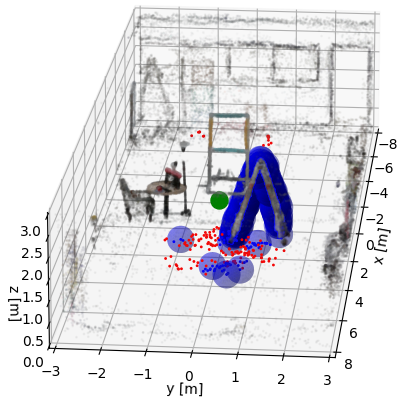
Figure 15: Visualization of the point cloud obtained from a Gaussian Splat of the test environment. For a quadcopter position (shown in green) near the ladder, we show (in blue) the union of balls $C(\epsilon)$ approximation to the nearby point cloud. We color nearby points blue if contained in $C(\epsilon)$ and red otherwise.

Visuomotor Quadcopter Policy Details

The policy used is an early version of [49]. The neural network has vision, command, and history portions. The vision portion processes (224, 224, 3) images via a fine-tuned SqueezeNet [66], then a multi-layer perceptron (MLP) of shape (512, 256, 128). The history network is a MLP of shape (32,16,8,2) trained to regress unknown quadcopter parameters from $5$ previous partial states (altitude, velocity, and orientation). Its penultimate output and vision network output are input to the command network which predicts an action using an MLP of shape (100, 100, 4). The history network is trained first and frozen. Then, the vision and command networks are jointly trained to match the expert action. Roughly $0.5*10^{6}$ state-action training pairs are used, obtained by perturbing the state from the desired trajectory and letting the expert controller run for $2$ [s]. We randomize mass, uniformly within $1.111\pm 0.2$ [kg], and thrust coefficient by $\pm 0.2$. We randomized position ([m]) and velocity ([m/s]) by $\pm 0.2$ and $\pm 0.1$ for orientation (here a quaternion). The policy runs at $50$ [hz] for $9$ [sec] when uninterrupted.

Baseline Classifier Details

We use [67] for all baselines except the neural network which is trained in PyTorch. The random forest uses 500 estimators, maximum depth of 8, and we use the output regression prediction as the conformal score. For the support vector machine (SVM), we use radial basis function (RBF) kernel, regularization $C=10^{4}$, and the signed distance from the decision boundary as the conformal score. For the neural network classifier, we use an MLP with ReLU activations, layer sizes $(9,100,50,25,1)$, and minimize with Adam binary cross-entropy loss over $50$ epochs with batch size of $256$.

Representation Learning Details

The autoencoder has encoder-decoder MLPs of shape $(7500,1000,600,400)$ and $(400,600,1000,7500)$, and minimizes reconstruction error with the Adam optimizer using batch size of $32$ for $50$ epochs. Figure 16 shows original and reconstructed images from the PCA and autoencoder. For PCA and KPCA, we subselect $15$ images from each safe trajectory but use all images in autoencoder training. After transforming, all safe images are used in two-sample conformal prediction except with CLIP (ViT-B/32 model) which uses $15$ from each safe trajectory due to large memory/compute overhead.

(a)

(b)

(c)

Figure 16: Original (top), autoencoder (middle), and PCA (bottom) reconstructions for images in a novel safe trajectory.

Proofs

Lemma .1 (Conformal Guarantee with Ties).

Let $S=\{s_{1},...,s_{N},s_{N+1}\}$ be exchangeable scores. Assume that almost surely at most $T$ of the scores share the same value (i.e., are tied). Then,

$$k/(N+1)\leq\Pr[s_{N+1}\leq s_{(k)}]\leq(k+T)/(N+1).$$ (34)

where $s_{(k)}$ is the $k$’th order statistic of $\{s_{1},...,s_{N}\}$.

Proof.

Imagine sorting $S$ in ascending order, breaking ties arbitrarily. Let the rank of $s_{i}$ denote its index in the sorted version of $S$. By exchangeability, $\Pr(s_{N+1}\mbox{ ranked }k)=1/(N+1)$ for each $k\in\{1,...,N+1\}$ implying

$$\Pr(s_{N+1}\mbox{ ranked }\leq k)=k/(N+1).$$ (35)

Let $Z_{1}=\sum_{i=1}^{N}\mathbbm{1}\left[s_{i}<s_{N+1}\right]$ count the number of scores strictly less than $s_{N+1}$ and $Z_{2}=\sum_{i=1}^{N}\mathbbm{1}\left[s_{i}=s_{N+1}\right]$ the number of scores tied with $s_{N+1}$. Since ties are split arbitrarily, the rank of $s_{N+1}$ is given by $Z_{1}+1+U$. Here $Z_{1}+1$ accounts for the fact that $s_{N+1}$ must appear after all $s_{i}$ strictly less than it and $U$ is a uniform random variable on $\{0,1,...,Z_{2}\}$ to model random tie splitting. With this notation, Eq. 35 becomes

$$\Pr(Z_{1}+1+U\leq k)=k/(N+1).$$ (36)

Since $s_{N+1}\leq s_{(k)}$ when at most $k-1$ of $s_{1},...,s_{N}$ violate $s_{N+1}\leq s_{i}$ (i.e., $s_{i}<s_{N+1}$ holds),

$$s_{N+1}\leq s_{(k)}\iff\sum_{i=1}^{N}\mathbbm{1}\left[s_{i}<s_{N+1}\right]\leq k-1.$$ (37)

Thus, in our notation

$$\Pr(s_{N+1}\leq s_{(k)})=\Pr(Z_{1}+1\leq k).$$ (38)

Since $0\leq U\leq Z_{2}\leq T$,

$$\Pr(Z_{1}+1\leq k)\geq\Pr(Z_{1}+1+U\leq k)$$ (39)

$$\geq\Pr(Z_{1}+1+T\leq k).$$

By Eq. 36,

$$\Pr(Z_{1}+1\leq k)\geq k/(N+1)\geq\Pr(Z_{1}+1\leq k-T).$$ (40)

Eq. 38 and the left side of Eq. 40 yield $\Pr(s_{N+1}\leq s_{(k)})\geq k/(N+1)$. Relabeling $k$ to $k+T$ in the right side of Eq. 40 and applying Eq. 38 yields

$$(k+T)/(N+1)\geq\Pr(Z_{1}+1\leq k)=\Pr(s_{N+1}\leq s_{(k)}).$$ (41)

∎

Lemma .2.

Consider sets $\{s_{1},...,s_{N}\}$ and $\{\alpha_{1},...,\alpha_{N}\}$. Suppose $\forall i:s_{N+1}\leq s_{i}\implies s_{N+1}\leq\alpha_{i}$. Then, $\forall k:s_{N+1}\leq s_{(k)}\implies s_{N+1}\leq\alpha_{(k)}$.

Proof.

Assuming $s_{N+1}\leq s_{(k)}$, $<k$ of $s_{1},...,s_{N}$ satisfy $s_{i}<s_{N+1}$, equivalently $>N-k$ satisfy $s_{N+1}\leq s_{i}$:

$$\sum_{i=1}^{N}\mathbbm{1}\left[s_{N+1}\leq s_{i}\right]>N-k.$$ (42)

Since $s_{N+1}\leq s_{i}\implies s_{N+1}\leq\alpha_{i}$,

$$\sum_{i=1}^{N}\mathbbm{1}\left[s_{N+1}\leq\alpha_{i}\right]>N-k\implies\sum_{i=1}^{N}\mathbbm{1}\left[\alpha_{i}<s_{N+1}\right]<k$$ (43)

and so $s_{N+1}\leq\alpha_{(k)}$. ∎

-A Proof of Theorem V.1

Proof.

Let $D_{-i}=\{x_{1},x_{2},...,x_{i-1},x,x_{i+1},...,x_{N}\}$ formed by swapping $x\coloneqq x_{N+1}$ into the $i$’th position of $D$. Consider the $i$-th score generated in full conformal prediction with the nearest neighbor score function (Eq. 7):

$$s_{i}^{x}=s(D_{-i};x_{i})=\min_{x^{\prime}\in D_{-i}}d(x^{\prime},x_{i})=$$ (44a)

$$\min\{\alpha_{i},d(x,x_{i})\}\leq\alpha_{i}$$ (44b)

by splitting to within the data $\alpha_{i}=\min_{x^{\prime}\in D,x^{\prime}\neq x_{i}}d(x^{\prime},x_{i})$ and with the test point $d(x,x_{i})$. Since $s_{i}^{x}\leq\alpha_{i}\ \forall i$,

$$s_{N+1}\leq s_{i}^{x}\implies s_{N+1}\leq\alpha_{i}$$ (45)

and so by Lemma .2,

$$s_{N+1}^{x}\leq s_{(k)}^{x}\implies s_{N+1}\leq\alpha_{(k)}.$$ (46)

Hence, also applying Lemma .1,

$$\Pr(s_{N+1}^{x}\leq\alpha_{(k)})\geq\Pr(s_{N+1}^{x}\leq s_{(k)}^{x})\geq k/(N+1).$$ (47)

$k=k(\epsilon)$ from Eq. 2 satisfies $k/(N+1)\geq 1-\epsilon$ so as $s_{N+1}^{x}=S(D;x)$, $\alpha_{(k)}=r$,

$$\Pr(s(D;x)\leq r)\geq 1-\epsilon.$$ (48)

∎

-B Proof of Theorem V.3

Proof.

Assuming no pairwise distance ties, almost surely (with probability 1) each $x_{i}$ has a unique nearest neighbor and $F$ has zero probability of repeatedly sampling a given point.

We’ll show that $Z_{2}$, the number of scores tied with $s_{N+1}^{x}$, has $Z_{2}\leq 1$ almost surely. Suppose not i.e., that $Z_{2}>1$. This requires that $\exists j\neq i\in\{1,...,N\}$ such that $s_{i}^{x}=s_{j}^{x}=s_{N+1}^{x}$. By above, $s_{i}^{x}$, $s_{j}^{x}$, and $s_{N+1}^{x}$ almost surely have unique minimizers $x_{i}^{*},x_{j}^{*},x_{N+1}^{*}$ (respectively) satisfying

$$d(x_{i}^{*},x_{i})=d(x_{j}^{*},x_{j})=d(x_{N+1}^{*},x_{N+1}).$$ (49)

By the no pairwise ties assumption, the event $d(x_{i}^{*},x_{i})=d(x_{j}^{*},x_{j})$ occurs (with nonzero probability) only when $x_{i}^{*}=x_{j},x_{j}^{*}=x_{i}$ (i.e., $x_{i}$ and $x_{j}$ are both each others nearest neighbors). Similarly, $d(x_{j}^{*},x_{j})=d(x_{N+1}^{*},x_{N+1})$ occurs only if $x_{j}^{*}=x_{N+1},x_{N+1}^{*}=x_{j}$. Therefore, $x_{j}^{*}=x_{i}$ and $x_{j}^{*}=x_{N+1}$ implying $x_{i}=x_{N+1}$. However, repeated sampling of the same point must occur with probability $0$. In summary, for the event $Z_{2}>1$ to occur requires conditions which occur with probability zero, so $Z_{2}\leq 1$ almost surely. Applying Lemma .1 with $T=1$ implies

$$\Pr(s_{N+1}^{x}\leq s_{(k)}^{x})\leq(k+1)/(N+1).$$ (50)

Since $d$ is symmetric,

$$s_{N+1}^{x}=\min_{j}d(x_{j},x)\leq d(x_{i},x)=d(x,x_{i}).$$ (51)

Hence, if $s_{N+1}^{x}\leq\alpha_{i}$, then $s_{N+1}^{x}\leq\min\{\alpha_{i},d(x,x_{i})\}=s_{i}^{x}$ (see Theorem V.1). Conclude $s_{N+1}^{x}\leq\alpha_{i}\implies s_{N+1}^{x}\leq s_{i}^{x}$. The converse also holds since $s_{i}^{x}\leq\alpha_{i}$ (see Theorem V.1) so

$$s_{N+1}\leq s_{i}^{x}\iff s_{N+1}\leq\alpha_{i}.$$ (52)

Applying Lemma .2 twice (for each implication direction),

$$s_{N+1}^{x}\leq s_{(k)}^{x}\iff s_{N+1}\leq\alpha_{(k)}$$ (53)

and so

$$\Pr(s_{N+1}^{x}\leq\alpha_{(k)})=\Pr(s_{N+1}^{x}\leq s_{(k)}^{x})\leq(k+1)/(N+1)$$ (54)

by Eq. 50.

$k(\epsilon)=\lceil(1-\epsilon)(N+1)\rceil\leq(1-\epsilon)(N+1)+1$ implies $\frac{k+1}{N+1}\leq(1-\epsilon)+2/(N+1)$. Eq. 54 with $s_{N+1}^{x}=S(D;x)$, $k=k(\epsilon),\alpha_{(k)}=r$ yields

$$\Pr(s(D;x)\leq r)\leq 1-\epsilon+2/(N+1).$$ (55)

∎

Remark.

In fact, this overcoverage bound can be tight. Taking $\epsilon\rightarrow 1$ from below yields $k(\epsilon)=1$ so that $C(\epsilon)$ is defined by $r=\alpha_{(1)}$ where following definition,

$$\alpha_{(1)}=\min_{x_{i}\neq x_{j}\in D}d(x_{i},x_{j})$$ (56)

$\alpha_{(2)}=\alpha_{(1)}$ as the minimizing $(x_{i},x_{j})$ pair each have an $\alpha_{i}$ and $\alpha_{j}$ term. Therefore, $r=\alpha_{(2)}$ so applying our analysis with $k=2$, conclude $C(\epsilon)$ provides at least $2/(N+1)$ coverage.

-C Proof of Theorem V.4

Proof.

Assuming $\{d(x_{i},x_{j})\}_{i,j}$ almost surely has no ties, the number of scores tied with $s_{N+1}^{x}$, defined as $Z_{2}$, equals zero almost surely. Applying Lemma .1 with $T=0$ yields

$$\Pr(s_{N+1}^{x}\leq s_{(k)}^{x})=\frac{k}{N+1}.$$ (57)

To bound the coverage we split into two cases:

$$\Pr(s_{N+1}^{x}\leq\alpha_{(k)})=\Pr(s_{N+1}^{x}\leq\alpha_{(k)},s_{(k)}^{x}\geq\alpha_{(k)})+$$ (58)

$$\Pr(s_{N+1}^{x}\leq\alpha_{(k)},s_{(k)}^{x}<\alpha_{(k)})$$

We bound the first term using Eq. 57:

$$\Pr(s_{N+1}^{x}\leq\alpha_{(k)},s_{(k)}^{x}\geq\alpha_{(k)})\leq$$ (59)

$$\Pr(s_{N+1}^{x}\leq s_{(k)}^{x},s_{(k)}^{x}\geq\alpha_{(k)})\leq$$

$$\Pr(s_{N+1}^{x}\leq s_{(k)}^{x})=\frac{k}{N+1}$$

We bound the second term by

$$\Pr(s_{N+1}^{x}\leq\alpha_{(k)},s_{(k)}^{x}<\alpha_{(k)})\leq\Pr(s_{(k)}^{x}<\alpha_{(k)}).$$ (60)

Imagine sorting $\alpha_{1},...,\alpha_{N}$ in ascending order yielding sorted indices $(i_{1},i_{2},...,i_{N})$ where $\alpha_{i_{k}}=\alpha_{(k)}$. Since $s_{i}^{x}\leq\alpha_{i}\ \forall i$ (Eq. 44), $s_{i_{j}}^{x}\leq\alpha_{i_{j}}$ for $j<k$. As there are almost surely no distance ties, $\alpha_{i_{j}}<\alpha_{i_{k}}$ yielding for $j<k$, $s_{i_{j}}^{x}<\alpha_{i_{k}}=\alpha_{(k)}$ almost surely. Thus, ignoring zero probability events,

$$s_{(k)}^{x}<\alpha_{(k)}\iff\exists i_{j},j\geq k:s_{i_{j}}^{x}<\alpha_{i_{k}}\iff$$ (61a)

$$\min\{s_{i_{j}}^{x}\}_{j=k:N}<\min\{\alpha_{i_{j}}\}_{j=k:N}.$$ (61b)

Consider the distances used in forming $s_{i_{j}}^{x}$ and $\alpha_{i_{j}}$ for $j=k,...,N$. For each $j$, $\alpha_{i_{j}}$ takes the minimum over $N-1$ terms $D_{j}^{\alpha}:=\{d(x_{i},x_{i_{j}})\}_{i=1:N,i\neq i_{j}}$ while $s_{i_{j}}^{x}$ takes the minimum over $N$ terms $D_{j}^{s}=D_{j}^{\alpha}\cup\{d(x_{N+1},x_{i_{j}})\}$. Therefore, $\min\{s_{i_{j}}^{x}\}_{j=k:N}$ is the minimum distance among $(N-k+1)N$ distances $D^{s}:=\cup_{j=k:N}D_{j}^{s}$ while $\min\{\alpha_{i_{j}}\}_{j=k:N}$ is the minimum distance among a subset $D^{\alpha}:=\cup_{j=k:N}D_{j}^{\alpha}\subset D^{s}$ of size $(N-k+1)(N-1)$. When $\min\{s_{i_{j}}^{x}\}_{j=k:N}\in D^{s}-D^{\alpha}$, $\min\{s_{i_{j}}^{x}\}_{j=k:N}<\min\{\alpha_{i_{j}}\}_{j=k:N}$ (otherwise they are equal). Since each distance is equally likely to be the minimizer $\min\{s_{i_{j}}^{x}\}_{j=k:N}$, simply counting yields

$$\Pr(\min\{s_{i_{j}}^{x}\}_{j=k:N}<\min\{\alpha_{i_{j}}\}_{j=k:N})=$$ (62a)

$$\Pr(\min\{s_{i_{j}}^{x}\}_{j=k:N}\in D^{s}-D^{\alpha})=$$ (62b)

$$\frac{(N-k+1)N-(N-k+1)(N-1)}{(N-k+1)N}=1/N.$$ (62c)

Using the equivalence in Eq. 61, conclude

$$\Pr(s_{(k)}^{x}<\alpha_{(k)})=1/N.$$ (63)

Combining with our bound on the first term,

$$\Pr(s_{N+1}^{x}\leq\alpha_{(k)}^{x})\leq k/(N+1)+1/N$$ (64)

Using $k(\epsilon)$ as in Eq. 2 implies $\frac{k}{N+1}\leq 1-\epsilon+1/(N+1)$. Eq. 64 with $s_{N+1}^{x}=S(D;x)$, $k=k(\epsilon),\alpha_{(k)}=r$ yields

$$\Pr(s(D;x)\leq r)\leq 1-\epsilon+1/(N+1)+1/N.$$ (65)

∎

-D Proof of Theorem V.2

Proof.

The condition $s(D;x)\leq r$ defining $C(\epsilon)$ means

$$\min_{x^{\prime}\in D}d(x^{\prime},x)\leq r\iff\exists i\in\{1,...,N\}:d(x_{i},x)\leq r$$ (66)

Grouping by $x_{i}$, we get each set $C_{i}$ by requiring $d(x_{i},x)\leq r$, yielding $C(\epsilon)$ as the union of $C_{i}$ sets. ∎

Appendix A Biography Section

Aaron O. Feldman received the B.S. degree in Information and Data Sciences from the California Institute of Technology in 2022 and is now pursuing a Ph.D. degree in Aeronautics and Astronautics at Stanford University. His current research focuses on statistical methods to guarantee safety and improve performance for robotic systems operating under uncertainty.

Joseph A. Vincent received a B.S. degree in Aerospace Engineering from the University of Kansas in 2018, and M.S. and Ph.D. degrees in Aeronautics and Astronautics from Stanford University in 2020 and 2024, respectively. His research interests include evaluation of robotic systems using statistical and reachability-based methods.

Maximilian Adang received a B.S. degree in Mechanical Engineering from the California Institute of Technology in 2023 and is now a Ph.D. student in Aeronautics and Astronautics at Stanford University. His research investigates the application of end-to-end machine learning methods to guidance, navigation, and control systems used in UAVs and robotic manipulation on-orbit.

Jun En Low is a graduate student in Mechanical Engineering at Stanford University. He received his B.Eng from the Singapore University of Technology and Design (SUTD) in 2015 where he worked on the dynamic modeling and control of unmanned aerial vehicles (UAVs). His current research interests are focused on zero-shot and end-to-end behavior cloning of visuomotor policies for UAVs.

Mac Schwager (Senior Member, IEEE) is Associate Professor of Aeronautics and Astronautics at Stanford University. He received a B.S. degree in Mechanical Engineering from Stanford University in 2000, and M.S. and Ph.D. degrees in Mechanical Engineering from the Massachusetts Institute of Technology in 2005 and 2009, respectively. His research interests include distributed algorithms for control, perception, and learning in groups of robots, and models of cooperation and competition in groups of engineered and natural agents. Dr. Schwager was the recipient of the NSF CAREER Award in 2014, the DARPA Young Faculty Award in 2018, and a Google Faculty Research Award in 2018, and the IROS Toshio Fukuda Young Professional Award in 2019.

References

- [1] D. R. Scobee and S. S. Sastry, “Maximum likelihood constraint inference for inverse reinforcement learning,” in International Conference on Learning Representations, 2020.
- [2] K. C. Stocking, D. L. McPherson, R. P. Matthew, and C. J. Tomlin, “Discretizing dynamics for maximum likelihood constraint inference,” arXiv preprint arXiv:2109.04874, 2021.
- [3] K. C. Stocking, D. L. McPherson, R. P. Matthew, and C. J. Tomlin, “Maximum likelihood constraint inference on continuous state spaces,” in 2022 International Conference on Robotics and Automation (ICRA), pp. 8598–8604, 2022.
- [4] S. Malik, U. Anwar, A. Aghasi, and A. Ahmed, “Inverse constrained reinforcement learning,” in International Conference on Machine Learning, pp. 7390–7399, PMLR, 2021.
- [5] G. Chou, D. Berenson, and N. Ozay, “Learning constraints from demonstrations,” in Algorithmic Foundations of Robotics XIII: Proceedings of the 13th Workshop on the Algorithmic Foundations of Robotics 13, pp. 228–245, Springer, 2020.
- [6] G. Chou, N. Ozay, and D. Berenson, “Learning parametric constraints in high dimensions from demonstrations,” in Conference on Robot Learning, pp. 1211–1230, PMLR, 2020.
- [7] G. Chou, N. Ozay, and D. Berenson, “Learning constraints from locally-optimal demonstrations under cost function uncertainty,” IEEE Robotics and Automation Letters, vol. 5, no. 2, pp. 3682–3690, 2020.
- [8] G. Chou, H. Wang, and D. Berenson, “Gaussian process constraint learning for scalable chance-constrained motion planning from demonstrations,” IEEE Robotics and Automation Letters, vol. 7, no. 2, pp. 3827–3834, 2022.
- [9] K. Srinivasan, B. Eysenbach, S. Ha, J. Tan, and C. Finn, “Learning to be safe: Deep rl with a safety critic,” arXiv preprint arXiv:2010.14603, 2020.
- [10] H. Bharadhwaj, A. Kumar, N. Rhinehart, S. Levine, F. Shkurti, and A. Garg, “Conservative safety critics for exploration,” in International Conference on Learning Representations, 2021.
- [11] S. Poletti, A. Testolin, and S. Tschiatschek, “Learning constraints from human stop-feedback in reinforcement learning,” AAMAS ’23, (Richland, SC), p. 2328–2330, International Foundation for Autonomous Agents and Multiagent Systems, 2023.
- [12] B. Thananjeyan, A. Balakrishna, S. Nair, M. Luo, K. Srinivasan, M. Hwang, J. E. Gonzalez, J. Ibarz, C. Finn, and K. Goldberg, “Recovery rl: Safe reinforcement learning with learned recovery zones,” IEEE Robotics and Automation Letters, vol. 6, no. 3, pp. 4915–4922, 2021.
- [13] B. Thananjeyan, A. Balakrishna, U. Rosolia, F. Li, R. McAllister, J. E. Gonzalez, S. Levine, F. Borrelli, and K. Goldberg, “Safety augmented value estimation from demonstrations (saved): Safe deep model-based rl for sparse cost robotic tasks,” IEEE Robotics and Automation Letters, vol. 5, no. 2, pp. 3612–3619, 2020.
- [14] J. Spencer, S. Choudhury, M. Barnes, M. Schmittle, M. Chiang, P. Ramadge, and S. Srinivasa, “Expert intervention learning: An online framework for robot learning from explicit and implicit human feedback,” Autonomous Robots, pp. 1–15, 2022.
- [15] Z. Xie, W. Zhang, Y. Ren, Z. Wang, G. J. Pappas, and W. Jin, “Safe mpc alignment with human directional feedback,” arXiv preprint arXiv:2407.04216, 2024.
- [16] N. Mehr, R. Horowitz, and A. D. Dragan, “Inferring and assisting with constraints in shared autonomy,” in 2016 IEEE 55th Conference on Decision and Control (CDC), pp. 6689–6696, 2016.
- [17] M. Saveriano and D. Lee, “Learning barrier functions for constrained motion planning with dynamical systems,” in 2019 IEEE/RSJ International Conference on Intelligent Robots and Systems (IROS), IEEE, nov 2019.
- [18] R. Laxhammar and G. Falkman, “Conformal prediction for distribution-independent anomaly detection in streaming vessel data,” in Proceedings of the first international workshop on novel data stream pattern mining techniques, pp. 47–55, 2010.
- [19] R. Laxhammar and G. Falkman, “Sequential conformal anomaly detection in trajectories based on hausdorff distance,” in 14th international conference on information fusion, pp. 1–8, IEEE, 2011.
- [20] J. Smith, I. Nouretdinov, R. Craddock, C. Offer, and A. Gammerman, “Anomaly detection of trajectories with kernel density estimation by conformal prediction,” in Artificial Intelligence Applications and Innovations: AIAI 2014 Workshops: CoPA, MHDW, IIVC, and MT4BD, Rhodes, Greece, September 19-21, 2014. Proceedings 10, pp. 271–280, Springer, 2014.
- [21] P. Contreras, O. Shorinwa, and M. Schwager, “Out-of-distribution runtime adaptation with conformalized neural network ensembles,” arXiv preprint arXiv:2406.02436, 2024.
- [22] R. Sinha, E. Schmerling, and M. Pavone, “Closing the loop on runtime monitors with fallback-safe mpc,” in 2023 62nd IEEE Conference on Decision and Control (CDC), pp. 6533–6540, IEEE, 2023.
- [23] R. Luo, S. Zhao, J. Kuck, B. Ivanovic, S. Savarese, E. Schmerling, and M. Pavone, “Sample-efficient safety assurances using conformal prediction,” The International Journal of Robotics Research, vol. 43, no. 9, pp. 1409–1424, 2024.
- [24] L. Lindemann, M. Cleaveland, G. Shim, and G. J. Pappas, “Safe planning in dynamic environments using conformal prediction,” IEEE Robotics and Automation Letters, 2023.
- [25] K. J. Strawn, N. Ayanian, and L. Lindemann, “Conformal predictive safety filter for rl controllers in dynamic environments,” IEEE Robotics and Automation Letters, 2023.
- [26] M. Cleaveland, I. Lee, G. J. Pappas, and L. Lindemann, “Conformal prediction regions for time series using linear complementarity programming,” in Proceedings of the AAAI Conference on Artificial Intelligence, vol. 38, pp. 20984–20992, 2024.
- [27] C. Stamouli, L. Lindemann, and G. Pappas, “Recursively feasible shrinking-horizon mpc in dynamic environments with conformal prediction guarantees,” in 6th Annual Learning for Dynamics & Control Conference, pp. 1330–1342, PMLR, 2024.
- [28] A. Dixit, L. Lindemann, S. X. Wei, M. Cleaveland, G. J. Pappas, and J. W. Burdick, “Adaptive conformal prediction for motion planning among dynamic agents,” in Learning for Dynamics and Control Conference, pp. 300–314, PMLR, 2023.
- [29] I. Gibbs and E. Candes, “Adaptive conformal inference under distribution shift,” Advances in Neural Information Processing Systems, vol. 34, pp. 1660–1672, 2021.
- [30] A. Muthali, H. Shen, S. Deglurkar, M. H. Lim, R. Roelofs, A. Faust, and C. Tomlin, “Multi-agent reachability calibration with conformal prediction,” in 2023 62nd IEEE Conference on Decision and Control (CDC), pp. 6596–6603, IEEE, 2023.
- [31] I. Gibbs and E. J. Candès, “Conformal inference for online prediction with arbitrary distribution shifts,” Journal of Machine Learning Research, vol. 25, no. 162, pp. 1–36, 2024.
- [32] A. Angelopoulos, E. Candes, and R. J. Tibshirani, “Conformal pid control for time series prediction,” Advances in neural information processing systems, vol. 36, 2024.
- [33] G. Shafer and V. Vovk, “A tutorial on conformal prediction.,” Journal of Machine Learning Research, vol. 9, no. 3, 2008.
- [34] A. N. Angelopoulos and S. Bates, “A gentle introduction to conformal prediction and distribution-free uncertainty quantification,” arXiv preprint arXiv:2107.07511, 2021.
- [35] H. Papadopoulos, K. Proedrou, V. Vovk, and A. Gammerman, “Inductive confidence machines for regression,” in Machine learning: ECML 2002: 13th European conference on machine learning Helsinki, Finland, August 19–23, 2002 proceedings 13, pp. 345–356, Springer, 2002.
- [36] R. Hulsman, “Distribution-free finite-sample guarantees and split conformal prediction,” Master’s thesis, Department of Statistics, University of Oxford, 2022.
- [37] A. Gammerman, V. Vovk, and V. Vapnik, “Learning by transduction,” in Proceedings of the Fourteenth Conference on Uncertainty in Artificial Intelligence, UAI’98, (San Francisco, CA, USA), p. 148–155, Morgan Kaufmann Publishers Inc., 1998.
- [38] V. Vovk, “Cross-conformal predictors,” Annals of Mathematics and Artificial Intelligence, vol. 74, pp. 9–28, 2015.
- [39] E. Ndiaye and I. Takeuchi, “Computing full conformal prediction set with approximate homotopy,” Advances in Neural Information Processing Systems, vol. 32, 2019.
- [40] E. Ndiaye and I. Takeuchi, “Root-finding approaches for computing conformal prediction set,” Machine Learning, vol. 112, 11 2022.
- [41] M. A. Turk and A. P. Pentland, “Face recognition using eigenfaces,” in Proc. IEEE Conference on Computer Vision and Pattern Recognition, pp. 586–591, 1991.
- [42] M.-H. Yang, N. Ahuja, and D. Kriegman, “Face recognition using kernel eigenfaces,” in Proceedings 2000 International Conference on Image Processing (Cat. No.00CH37101), vol. 1, pp. 37–40 vol.1, 2000.
- [43] K. Q. Weinberger, J. Blitzer, and L. Saul, “Distance metric learning for large margin nearest neighbor classification,” in Advances in Neural Information Processing Systems (Y. Weiss, B. Schölkopf, and J. Platt, eds.), vol. 18, MIT Press, 2005.
- [44] M. Caron, H. Touvron, I. Misra, H. Jégou, J. Mairal, P. Bojanowski, and A. Joulin, “Emerging properties in self-supervised vision transformers,” in Proceedings of the IEEE/CVF international conference on computer vision, pp. 9650–9660, 2021.
- [45] M. Oquab, T. Darcet, T. Moutakanni, H. Vo, M. Szafraniec, V. Khalidov, P. Fernandez, D. Haziza, F. Massa, A. El-Nouby, et al., “Dinov2: Learning robust visual features without supervision,” arXiv preprint arXiv:2304.07193, 2023.
- [46] A. Radford, J. W. Kim, C. Hallacy, A. Ramesh, G. Goh, S. Agarwal, G. Sastry, A. Askell, P. Mishkin, J. Clark, et al., “Learning transferable visual models from natural language supervision,” in International conference on machine learning, pp. 8748–8763, PMLR, 2021.
- [47] S. Maneewongvatana and D. M. Mount, “Analysis of approximate nearest neighbor searching with clustered point sets,” arXiv preprint cs/9901013, 1999.
- [48] J. A. Vincent, A. O. Feldman, and M. Schwager, “Guarantees on robot system performance using stochastic simulation rollouts,” IEEE Transactions on Robotics, 2024.
- [49] J. Low, M. Adang, J. Yu, K. Nagami, and M. Schwager, “SOUS VIDE: Cooking visual drone navigation policies in a gaussian splatting vacuum,” 2024. In Preparation.
- [50] V. Ye, R. Li, J. Kerr, M. Turkulainen, B. Yi, Z. Pan, O. Seiskari, J. Ye, J. Hu, M. Tancik, et al., “gsplat: An open-source library for gaussian splatting,” arXiv preprint arXiv:2409.06765, 2024.
- [51] M. Tancik, E. Weber, E. Ng, R. Li, B. Yi, T. Wang, A. Kristoffersen, J. Austin, K. Salahi, A. Ahuja, et al., “Nerfstudio: A modular framework for neural radiance field development,” in ACM SIGGRAPH 2023 Conference Proceedings, pp. 1–12, 2023.
- [52] R. Verschueren, G. Frison, D. Kouzoupis, J. Frey, N. v. Duijkeren, A. Zanelli, B. Novoselnik, T. Albin, R. Quirynen, and M. Diehl, “acados—a modular open-source framework for fast embedded optimal control,” Mathematical Programming Computation, vol. 14, no. 1, pp. 147–183, 2022.
- [53] B. Landry, R. Deits, P. R. Florence, and R. Tedrake, “Aggressive quadrotor flight through cluttered environments using mixed integer programming,” in 2016 IEEE international conference on robotics and automation (ICRA), pp. 1469–1475, IEEE, 2016.
- [54] X. Zhang, A. Liniger, and F. Borrelli, “Optimization-based collision avoidance,” IEEE Transactions on Control Systems Technology, vol. 29, no. 3, pp. 972–983, 2020.
- [55] A. Cauligi, P. Culbertson, E. Schmerling, M. Schwager, B. Stellato, and M. Pavone, “Coco: Online mixed-integer control via supervised learning,” IEEE Robotics and Automation Letters, vol. 7, no. 2, pp. 1447–1454, 2021.
- [56] T. Marcucci, M. Petersen, D. von Wrangel, and R. Tedrake, “Motion planning around obstacles with convex optimization,” Science robotics, vol. 8, no. 84, p. eadf7843, 2023.
- [57] T. Chen, A. Swann, J. Yu, O. Shorinwa, R. Murai, M. Kennedy III, and M. Schwager, “Safer-splat: A control barrier function for safe navigation with online gaussian splatting maps,” arXiv preprint arXiv:2409.09868, 2024.
- [58] T. Chen, O. Shorinwa, J. Bruno, J. Yu, W. Zeng, K. Nagami, P. Dames, and M. Schwager, “Splat-nav: Safe real-time robot navigation in gaussian splatting maps,” arXiv preprint arXiv:2403.02751, 2024.
- [59] R. J. Tibshirani, R. Foygel Barber, E. Candes, and A. Ramdas, “Conformal prediction under covariate shift,” Advances in neural information processing systems, vol. 32, 2019.
- [60] R. J. Moss, M. J. Kochenderfer, M. Gariel, and A. Dubois, “Bayesian safety validation for failure probability estimation of black-box systems,” Journal of Aerospace Information Systems, pp. 1–14, 2024.
- [61] H. Akaike, “An approximation to the density function,” Annals of the Institute of Statistical Mathematics, vol. 6, no. 2, pp. 127–132, 1954.
- [62] G. Biau, L. Devroye, G. Biau, and L. Devroye, “The k-nearest neighbor density estimate,” Lectures on the Nearest Neighbor Method, pp. 25–32, 2015.
- [63] P. Zhao and L. Lai, “Analysis of knn density estimation,” IEEE Transactions on Information Theory, vol. 68, no. 12, pp. 7971–7995, 2022.
- [64] J. Lei, J. M. Robins, and L. A. Wasserman, “Distribution-free prediction sets,” Journal of the American Statistical Association, vol. 108, pp. 278 – 287, 2013.
- [65] A. M. Mood, F. A. Graybill, and D. C. Boes, Introduction to the Theory of Statistics. McGraw-Hill, 3rd ed., 1974.
- [66] F. N. Iandola, “Squeezenet: Alexnet-level accuracy with 50x fewer parameters and 0.5 mb model size,” arXiv preprint arXiv:1602.07360, 2016.
- [67] F. Pedregosa, G. Varoquaux, A. Gramfort, V. Michel, B. Thirion, O. Grisel, M. Blondel, P. Prettenhofer, R. Weiss, V. Dubourg, et al., “Scikit-learn: Machine learning in python,” the Journal of machine Learning research, vol. 12, pp. 2825–2830, 2011.