An Analysis of Model Robustness
across Concurrent Distribution Shifts

Abstract

Machine learning models, meticulously optimized for source data, often fail to predict target data when faced with distribution shifts (DSs). Previous benchmarking studies, though extensive, have mainly focused on simple DSs. Recognizing that DSs often occur in more complex forms in real-world scenarios, we broadened our study to include multiple concurrent shifts, such as unseen domain shifts combined with spurious correlations. We evaluated 26 algorithms that range from simple heuristic augmentations to zero-shot inference using foundation models, across 168 source-target pairs from eight datasets. Our analysis of over 100K models reveals that (i) concurrent DSs typically worsen performance compared to a single shift, with certain exceptions, (ii) if a model improves generalization for one distribution shift, it tends to be effective for others, and (iii) heuristic data augmentations achieve the best overall performance on both synthetic and real-world datasets.

1 Introduction

Machine learning models deployed in real-world settings may face complex distribution shifts (DSs). These shifts can result in unreliable predictions. For instance, a self-driving car may be deployed in a place where there is a different driving etiquette, unfamiliar environment and weather condition. Thus, a systematic evaluation of such complex shifts is essential before deploying models in the real world.

Most research has focused on evaluating models under a single DS (UniDS) (Taori et al., 2020; Gulrajani & Lopez-Paz, 2020; Koh et al., 2021; Wiles et al., 2022; Miller et al., 2021; Wenzel et al., 2022). For instance, in the PACS evaluation benchmark (Li et al., 2017), the training data consists of photographs, but the model is tested on sketches. Similarly, in the training data of Biased FFHQ (Lee et al., 2021), gender is spuriously correlated to age, but the model is tested on data where gender is anti-correlated to age. In a real-world scenario, we can encounter these two shifts concurrently, i.e., one where age and gender are spuriously correlated and where there is also a shift in the style of the image.

To address this, we introduce an evaluation framework that mirrors the complex DSs potentially found in real-world settings. We assume that the input is generated from a set of attributes, e.g., gender, age, image style, etc. Thus, we leverage existing multi-attribute datasets, such as CelebA (Karras et al., 2017), which includes 40 attribute labels such as gender, hair color, and smiling, to manipulate the type and number of DSs present in the dataset. We refer to this framework as ConDS. It can account for the co-occurrence of different DSs across multiple attributes within paired source and target datasets. An example of this protocol is illustrated in Figure 1. Consequently, evaluating existing methods against these shifts can provide insights unattainable with current benchmarks. Specifically, our proposed framework consists of the following components:

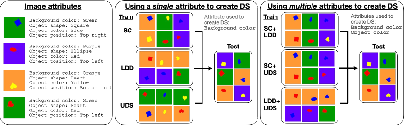
Figure 1: Concurrent distribution shifts. Left: We list some attributes of a few images from the dSprites dataset. In this dataset, the object shape is the label. Center: We show how a single attribute e.g., the background color, can be used to create different types of distribution shifts. Namely, spurious correlation (SC), where in this example, the background color is correlated with the object shape, low data drift (LDD), and unseen data shift (UDS). We assume that the test data consists of images where all attribute instances are equally likely to appear, i.e., each image is generated by randomly selecting each attribute instance with equal probability. Right: As the real world consists of more complex shifts, we also make use of multiple attributes to create combinations of distribution shifts. In the examples above, we use the background and object color to create combinations of distribution shifts. The first shift is created using the background attribute and the second shift, the shape attribute i.e., SC+UDS is created from a correlation between the background color and the shape (SC), and only using a subset of colors, for the shape attribute (UDS).

Distribution Shifts. We explore seven types of DSs, including spurious correlation (SC), low data drift (LDD), unseen data shift (UDS), and their combinations; that is, (SC, LDD), (SC, UDS), (LDD, UDS), and (SC, LDD, UDS). To offer a comprehensive analysis covering a wide range of cases, we select various attributes to induce DSs. This includes adjusting three attributes for each UniDS and creating six combinations from three attributes for each ConDS, resulting in 33 distinct cases per dataset.

Algorithms. We evaluate 26 different methods from 7 popular approaches: architectural strategies, data augmentations, de-biasing, worst-case generalization, single domain generalization, out-of-distribution generalization, and even zero-shot inference using vision-language foundation models.

Experiments. We evaluate these algorithms on all proposed combinations of DSs. This results in over 100K experiments across 168 dataset pairs sourced from 3 synthetic and 5 real-world benchmarks. Further, we examine aspects such as the effectiveness of pre-training and the influence of prompts on foundation models for image classification.

As a result, we have made some intriguing findings: (i) Concurrent shifts are generally more challenging than single shifts. However, in ConDS, when a particularly difficult DS is combined with relatively easier ones, the harder shift tends to dominate, limiting any further increase in overall difficulty. (ii) If a model improves generalization for one DS, it proves effective for others, even if it was originally designed to address a specific shift. (iii) Heuristic augmentation techniques outperform meticulously crafted generalization methods overall. (iv) Although vision-language foundation models (e.g., CLIP, LLaVA) perform well on simple datasets, even in the presence of DSs, their performance significantly deteriorates on more complex, real-world datasets.

2 Related Work

In this section, we review existing benchmarks for distribution shifts (DSs) and frameworks for evaluating model generalization.

Benchmarks.

Several types of benchmarks have been introduced to evaluate the generalization of models. One type of benchmark evaluates generalization on datasets collected from different sources, i.e., due to different domains (Li et al., 2017; Venkateswara et al., 2017; Peng et al., 2019; Koh et al., 2021) e.g., the train and test data are collected from different countries, or different time periods (Yao et al., 2022; Hendrycks et al., 2021). Another popular type applies transformations to the input (Hendrycks & Dietterich, 2019; Sagawa et al., 2019; Nam et al., 2020; Bahng et al., 2020; Jeon et al., 2022b). Such transformations range from analytical ones like rotation, corruptions like ‘brightness’ or ‘contrast’, to learned ones like adversarial attacks. Images with the same transformations form a domain, while each transformation can be an attribute, creating spurious correlations by matching labels to transformations. Other alternatives includes using engines like Blender or Unity to create simulators that can render different types of shifts (Leclerc et al., 2022; Sun et al., 2022). In contrast, Recht et al. (2019) collects new test sets for ImageNet and CIFAR-10 by replicating the data collection pipeline. They showed that without any explicit distribution shift, there is a drop in accuracy. Similarly, Barbu et al. (2019) collects a new dataset where objects have unusual poses or viewpoints. The benchmarks most similar to ours involve changing the original train-test split of the dataset to induce different types of DSs (Kim et al., 2019; Koh et al., 2021; Jeon et al., 2022a; Atanov et al., 2022; Jeon et al., 2022b). In contrast to these methods, our paper focuses on creating controllable concurrent shifts by using attribute annotations in existing datasets.

Large-scale Generalization Analysis.

Although methods that enhance robustness against DSs have been extensively researched, significant variations across application domains mean that a method that excels in one dataset might not perform equally well in another. Consequently, recent efforts have been dedicated to comprehensively and fairly evaluate generalization methods. Gulrajani & Lopez-Paz (2020) demonstrated that empirical risk minimization, when meticulously implemented and finely tuned, excels over domain generalization methods in robustness. Taori et al. (2020) found that generalizability to synthetic shifts does not guarantee robustness to natural shifts. Koh et al. (2021) introduced Wilds, a curated benchmark consisting of 10 datasets that encapsulate a diverse range of DSs encountered in real-world settings. Their findings indicate that current methods for generalization are inadequately equipped to address real-world DSs. Wiles et al. (2022) reported that both pre-training and augmentations significantly boost performance across many scenarios, although the most effective methods vary with different datasets and DSs. Additionally, Miller et al. (2021) and Wenzel et al. (2022) observed a positive correlation between out-of-distribution and in-distribution performance. However, these studies predominantly concentrate on single DSs, which do not fully capture real-world scenarios. Ye et al. (2022) categorized existing benchmarks based on the extent of spurious correlations and the degree of domain shift. Their findings reveal that, for the most part, Out-of-Distribution generalization algorithms remain susceptible to spurious correlations.

3 Problem Statement

In this section, we introduce the concept of distribution shift (DS) and its two categories: unique distribution shift (UniDS) and concurrent distribution shift (ConDS). To operationalize the concept of ConDS, annotations for multiple attributes are required. For clarity, we begin by introducing one of our experimental datasets, dSprites, in Figure 2.

3.1 Distribution Shift

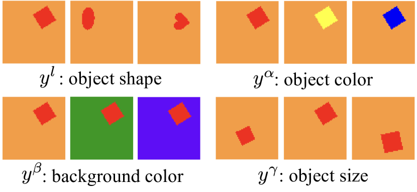
Figure 2: dSprites samples. Even in simple synthetic data, multiple attributes can potentially lead to various DSs. Visualizations for other datasets are included in Figure 5 in the Section A.1.

Consider an instance set $X=\{\mathbf{x}_{i}|\mathbf{x}_{i}\in\mathcal{X},i=1,\dots,N\}$ for a classification problem, where $\mathcal{X}$ denotes the input space. Each instance ${\bf x}$ can be represented by a finite set of attributes $Y({\bf x})=\{y^{k}|y^{k}\in{\cal Y},k=1,\dots,K\}$ where ${\cal Y}$ denotes the attribute space and $K$ varies with ${\bf x}$. Within this framework, one attribute $y^{l}$ from $Y({\bf x})$ can be designated as the label. Let $p$, $p_{S}$, and $p_{T}$ be the true, source, and target distributions, respectively. We denote the source and target datasets by $\mathcal{D}_{S}\sim p_{S}$ and $\mathcal{D}_{T}\sim p_{T}$, respectively, where each dataset consists of samples from its corresponding distribution. A machine learning model $\hat{f}$ is designed to minimize the empirical risk,

$$\hat{f}:=\operatorname*{arg\,min}_{f}\frac{1}{N}\sum_{i=1}^{N}\mathcal{L}(y_{i}^{l},f(\mathbf{x}_{i})),$$ (1)

where $(\mathbf{x}_{i},y_{i}^{l})\in\mathcal{D}_{S}$ for $i=1,...,N$. The ideal objective is to find the model $f^{*}$ that maximizes its performance on true distribution $p(\mathbf{x},y)$; that is,

$$f^{*}:=\operatorname*{arg\,min}_{\hat{f}}\mathbb{E}_{p(\mathbf{x},y^{l})}\left[\mathcal{L}(y^{l},\hat{f}(\mathbf{x}))\right].$$ (2)

However, a significant shift in distribution from source to target data, denoted by $\mathcal{D}_{S}\not\approx\mathcal{D}_{T}$, can cause a substantial decrease in performance during inference. Assuming that the target distribution $p_{T}$ aligns with $p$, we define DSs in the following subsections.

3.2 Unique Distribution Shifts

We revisit spurious correlation (SC), low data drift (LDD), and unseen data shift (UDS) as delineated in the experimental framework by Wiles et al. (2022), grouping these under the category of unique distribution shifts (UniDS), namely UniDS $:=$ {SC, LDD, UDS}. To create the UniDS, we select one attribute from the candidates ($y^{\alpha}$, $y^{\beta}$, $y^{\gamma}$) and then sample the images for each DS accordingly. All other attributes display a uniform distribution for UniDS.

Test distribution $p_{T}$. All the attributes $y^{k}\in Y({\bf x})$ are uniformly distributed, ensuring that each attribute is represented and independent from the others. For example, for $p_{T}\approx p$, there is an equal number of samples across 81 combinations, ranging from (square, red, orange, small) to (heart, blue, purple, big).

Spurious correlation. Under $p_{S}$, the label $y^{l}$ and a specific attribute $y^{\alpha}$ exhibit correlation, which does not hold under $p_{T}$. For example, there are only (square, red), (ellipse, yellow), and (heart, blue) samples in ${\cal D}_{S}$, exhibiting a correlation between ‘shape’ and ‘color’.

Low data drift. Attribute values show an uneven distribution under $p_{S}$ but are more evenly distributed under $p_{T}$. Generalization for LDD is also referred to as worst-case generalization (Sagawa et al., 2019; Seo et al., 2022). For example, there are significantly fewer red samples compared to the numerous yellow and blue samples. Even among the red samples, the distribution of shapes is uneven.

Unseen data shift. Some attribute values that are not present under $p_{S}$ appear under $p_{T}$. E.g., There are no blue images in ${\cal D}_{S}$, indicating that blue images in ${\cal D}_{T}$ are new to the model.

3.3 Concurrent Distribution Shifts

Previous benchmarking studies have predominantly focused on UniDS. However, in real-world contexts, a dataset could contain concurrent DSs. Given that an instance ${\bf x}$ encompasses numerous attributes, DSs can exhibit more complex structures, with each attribute governed by distinct UniDS. For instance, in the real-world dataset iWildCam, UDS are observed due to discrepancies in the camera traps used across source and target data. Concurrently, LDD emerges from variable image counts across animal classes. Therefore, to effectively assess the efficacy of methods in real-world applications, it is crucial to conduct a comprehensive evaluation that addresses these scenarios.

To reflect the complexities observed in real-world datasets, we introduce the concept of “concurrent distribution shift (ConDS)". This novel framework extends conventional UniDS by modeling the diverse shifts associated with different attributes of a dataset. In this study, we focus on combining various shifts attributed to different attributes, rather than evaluating a single type of shift across multiple attributes—a topic extensively covered in previous literature.

For instance, using the attributes shown in Figure 2, (SC, UDS) can be established by sampling combinations such as (square, red), (ellipse, yellow), and (heart, blue), while the background color varies between (orange, green) and the object size maintains a uniform distribution. The concept of ConDS and its importance were also introduced in Koh et al. (2021). However, their discussion was limited to LDD and UDS. We broaden this to include SC, LDD, and UDS, aiming for a thorough understanding of their interconnections. Additionally, we investigate a broader array of algorithms to assess how existing methods perform on ConDS.

4 Generalization to Distribution Shifts

As discussed in Section 3.1, it is assumed that during training, we only have access to source data, while the target distribution remains unknown (Vapnik, 1991; Jeon et al., 2023). While some algorithms are specifically designed for scenarios where partial knowledge of the target distribution is available (Adeli et al., 2021; Alvi et al., 2018; Kim et al., 2019; Geirhos et al., 2018; Bahng et al., 2020; Ganin et al., 2016), the setup where no target information is known generally poses a broader challenge for model generalization. Consequently, our analysis focuses on this more general setup. We evaluate 26 algorithms suitable for this scenario, spanning a wide spectrum of methods, as shown in Table 1.

Table 1: Generalization algorithms evaluated. We outline the methods evaluated and the distribution shifts they are designed to address.

Generalization Algorithms		SC	LDD	UDS
Architecture	ResNet18, ResNet50, ResNet101 (He et al., 2016),
	ViT (Dosovitskiy et al., 2020), MLP (Vapnik, 1991).
Heuristic augmentation	Imagenet (He et al., 2016), AugMix (Hendrycks et al., 2019),			✓
	RandAug (Cubuk et al., 2020), AutoAug (Cubuk et al., 2019).
De-biasing	UBNet (Jeon et al., 2022a), PnD (Li et al., 2023),	✓
	OccamNets (Shrestha et al., 2022).
Worst-case generalization	GroupDRO (Sagawa et al., 2019), BPA (Seo et al., 2022).		✓
Single domain generalization	ADA (Volpi et al., 2018), ME-ADA (Zhao et al., 2020),			✓
	SagNet (Nam et al., 2021), L2D (Wang et al., 2021).
Out-of-distribution generalization	IRM (Arjovsky et al., 2019), CausIRL (Chevalley et al., 2022).	✓	✓	✓
Zero-shot inference with foundation model	CLIP (Radford et al., 2021), InstructBLIP (Dai et al., 2024),
	LLaVA-1.5 (Liu et al., 2023), Phi-3.5-vision (Abdin et al., 2024),
	GPT-4o-mini, GPT-4o (OpenAI, 2024).

Augmentation for generalization. Although some augmentation techniques are not specifically designed for robustness, they are commonly used to enhance generalization against the unseen domain and are well known for their effectiveness (Yan et al., 2020; Wiles et al., 2022; Cugu et al., 2022; Zheng et al., 2024). The operative idea is that augmentation expands the input space, thereby increasing the likelihood that the model will recognize new test samples.

Generalization algorithms. De-biasing: UBNet utilizes feature maps from lower to higher layers to enable the model to access a broader feature space. PnD removes spurious correlations by detecting them using GCE (Zhang & Sabuncu, 2018). OccamNets employs architectural inductive biases, demonstrating their effectiveness in mitigating spurious correlations. Worst-case generalization: GroupDRO and BPA modify the weight of gradient flow to ensure balance across different groups. Single domain generalization: ADA and ME-ADA generate additional inputs by incorporating adversarial noise. SagNet is designed to be agnostic to styles, emphasizing content instead. L2D utilizes learned augmentations with AdaIN from StyleGAN (Karras et al., 2019). Out-of-distribution generalization: IRM and CausIR eliminate variant features by regularizing discrepancies among samples from the source data.

Foundation model for image classification. Foundation models acquire robust representations from comprehensive datasets, facilitating their application in downstream tasks such as image classification. The mechanisms for aligning inputs to outputs (${\cal X}\rightarrow{\cal Y}$) during zero-shot inference differ among models. CLIP utilizes the similarity between image embeddings and textual label embeddings to calculate confidence scores. Conversely, InstructBLIP, LLaVA-1.5, Phi-3.5-vision, and GPT-4o employ label-eliciting prompts as queries within the framework of visual question answering (Chen et al., 2022). Additional details about the prompts used for image classification can be found in Table 12 of the Section B.5.

5 Experiments

In this section, we begin by presenting the datasets we evaluated on and the experimental setup. Next, we evaluated 26 distinct algorithms across 168 (source, target) pairs spanning six datasets, addressing both UniDS and ConDS. The aggregate results are illustrated in Figure 3, while the comprehensive results are detailed in Section B.1. We further examine how the challenges vary among different DSs (Figure 4) and evaluate the effectiveness of pre-training in enhancing robustness (Table 3). Further analysis investigates how zero-shot inference performance depends on distribution shifts (DSs), as shown in Table 5. Finally, we analyze the outcomes, summarizing them into eight key takeaways.

Table 2: Attributes for controlled datasets. Each dataset’s attributes and their possible values. Image samples from each dataset are displayed in Figure 5 in Section A.1.

Dataset	Attribute		Values
dSprites	$y^{l}$	object shape	{square, ellipse, heart}
	$y^{\alpha}$	object color	{red, yellow, blue}
	$y^{\beta}$	background color	{orange, green, purple}
	$y^{\gamma}$	object size	{small, middle, big}
Shapes3D	$y^{l}$	object shape	{cube, cylinder, sphere, capsule}
	$y^{\alpha}$	object color	{red, orange, yellow, green}
	$y^{\beta}$	background color	{red, orange, yellow, green}
	$y^{\gamma}$	object size	{tiny, small, middle, big}
SmallNorb	$y^{l}$	object	{animal, human, car, truck, airplane}
	$y^{\alpha}$	azimuth	{0, 80, 160, 240, 320}
	$y^{\beta}$	lighting	{0, 1, 2, 3, 4}
	$y^{\gamma}$	elevation	{30, 40, 50, 60, 70}
CelebA	$y^{l}$	gender	{male, female}
	$y^{\alpha}$	hair color	{black, others}
	$y^{\beta}$	smiling	{smiling, no smiling}
	$y^{\gamma}$	hair style	{straight, others}
DeepFashion	$y^{l}$	dress	{skirt, others}
	$y^{\alpha}$	pattern	{floral, solid}
	$y^{\beta}$	sleeve	{long sleeve, sleeveless}
	$y^{\gamma}$	fabric	{chiffon, cotton}

5.1 Datasets

Controlled datasets: We assess algorithms using five evaluation datasets: dSprites, Shapes3D, SmallNorb, CelebA, and DeepFashion. From these, we select four attributes: one is designated as the label ($y^{l}$), and the other three as attributes ($y^{\alpha}$, $y^{\beta}$, $y^{\gamma}$) to create DSs. Table 2 lists the attribute instances for $y^{l}$ and $\{y^{\alpha},y^{\beta},y^{\gamma}\}$ for the different controlled datasets. We divide the source data into training and validation sets, both sharing the same distribution, with the validation set used for hyperparameter tuning.

Uncontrolled real-world datasets: We use iWildCam, fMoW, and Camelyon17 for evaluation. iWildCam data in the Wilds benchmark (Koh et al., 2021) exhibits LDD over the animal distributions, and UDS occurs across camera trap locations. Similarly, the fMoW dataset (Koh et al., 2021) exhibits UDS and LDD across time and regions in satellite images. Camelyon17 is a tumor detection dataset with various unexpected DSs resulting from different hospitals. We further discuss additional insights from the categorization of synthetic (Dsprites, Shapes3D, Smallnorb) and real-world datasets (CelebA, DeepFashion, iWildCam, fMoW, Camelyon17) in Section A.3.

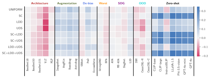
Figure 3: Aggregate result on controlled datasets. We plot the change in accuracy compared to the base model, ResNet18, averaged across all seeds and controlled datasets with varying attributes. Blue indicates improved performance, while red indicates a decline. Each row is independent of the others. The models used for zero-shot inference were only used for evaluation, thus, they have the same absolute performance for each row. However, as we show their accuracies relative to the ResNet18, the relative performance for each model is not the same for each row. We fine-tune all the algorithms and report their optimal results. Augmentation methods and zero-shot models perform well under the different types of shifts. We provide a breakdown of the accuracy for each algorithm and dataset in the Section B.1.

Table 3: Training from scratch vs Pre-training. All the values reported for controlled datasets represent the average accuracy across all DSs and controlled datasets. We compare the performance of models trained from scratch with those pre-trained, bolding the better result between the two training strategies. The top average result in each column except zero-shot inference is indicated with a gray box, while the second-best is underlined. We used the original models for zero-shot inference for evaluations, thus, they are neither trained from scratch nor fine-tuned. Trends on controlled datasets vs Real-world datasets. We also show the results from evaluating on iWildCam, fMoW, and Camelyon17, as they are challenging real-world datasets with ConDS. The experimental results from our controlled datasets align with those from the real-world datasets, demonstrating that even on real-world datasets, augmentation and pre-training significantly enhance robustness.

		Controlled Dataset		Real-world Dataset
		Scratch	Pre-training	Scratch	Pre-training
Architecture	ResNet18	62.43($\pm$0.84)	81.53($\pm$0.67)	53.91($\pm$2.19)	61.64($\pm$1.71)
	ResNet50	60.13($\pm$0.85)	82.64($\pm$0.62)	52.58($\pm$1.86)	67.76($\pm$1.46)
	ResNet101	56.98($\pm$0.88)	79.96($\pm$0.69)	47.01($\pm$2.09)	67.52($\pm$1.41)
	ViT	49.55($\pm$0.60)	78.53($\pm$0.62)	50.55($\pm$2.11)	70.94($\pm$1.55)
	avg.	57.27($\pm$2.81)	80.67($\pm$0.90)	51.01($\pm$1.50)	66.97($\pm$1.94)
Augmentation	ImageNet	69.25($\pm$0.88)	80.55($\pm$0.64)	48.82($\pm$1.80)	66.48($\pm$1.60)
	AugMix	68.99($\pm$0.83)	83.15($\pm$0.56)	51.99($\pm$1.74)	68.09($\pm$1.53)
	RandomAug	71.47($\pm$0.86)	85.28($\pm$0.53)	51.94($\pm$1.84)	68.29($\pm$1.62)
	AutoAug	69.65($\pm$0.85)	85.85($\pm$0.53)	52.15($\pm$1.63)	70.29($\pm$1.59)
	avg.	69.84($\pm$0.56)	83.71($\pm$1.20)	51.22($\pm$0.80)	68.29($\pm$0.78)
De-biasing	UBNet	61.08($\pm$0.86)	78.26($\pm$0.67)	41.01($\pm$2.32)	59.03($\pm$1.77)
	PnD	68.15($\pm$0.87)	77.67($\pm$0.79)	50.02($\pm$2.49)	60.34($\pm$1.55)
	OccamNets	64.98($\pm$0.71)	77.59($\pm$0.68)	52.57($\pm$1.80)	65.20($\pm$1.39)
	avg.	64.74($\pm$2.04)	77.84($\pm$0.21)	47.87($\pm$3.51)	61.52($\pm$1.88)
Worst-case generalization	GroupDRO	63.26($\pm$0.84)	81.23($\pm$0.67)	48.17($\pm$1.87)	64.40($\pm$1.26)
	BPA	59.99($\pm$0.81)	75.69($\pm$0.74)	40.41($\pm$3.93)	62.15($\pm$1.69)
	avg.	61.63($\pm$1.63)	78.46($\pm$2.77)	44.29($\pm$3.88)	63.28($\pm$1.13)
Single domain generalization	ADA	62.98($\pm$0.82)	80.20($\pm$0.68)	52.88($\pm$2.02)	69.71($\pm$1.51)
	ME-ADA	62.37($\pm$0.82)	78.33($\pm$0.69)	53.79($\pm$2.04)	66.41($\pm$1.20)
	SagNet	61.09($\pm$0.86)	81.56($\pm$0.67)	54.27($\pm$1.93)	66.75($\pm$1.27)
	L2D	66.42($\pm$0.83)	82.63($\pm$0.60)	52.67($\pm$2.47)	68.20($\pm$1.95)
	avg.	63.22($\pm$1.14)	80.68($\pm$0.93)	53.40($\pm$0.38)	67.77($\pm$0.75)
Out-of-distribution generalization	IRM	59.83($\pm$0.83)	80.27($\pm$0.68)	39.47($\pm$2.42)	57.90($\pm$2.14)
	CausIRL-M	57.55($\pm$0.98)	80.81($\pm$0.75)	48.90($\pm$1.97)	65.87($\pm$1.21)
	CausIRL-C	64.17($\pm$0.85)	82.02($\pm$0.68)	54.38($\pm$2.07)	68.06($\pm$1.55)
	avg.	60.52($\pm$1.94)	81.03($\pm$0.52)	47.58($\pm$4.35)	63.94($\pm$3.09)
Zero-shot inference	CLIP-base	78.92		25.76
	CLIP-large	86.22		29.06
	InstructBLIP	70.95		29.35
	LLaVA-1.5	88.24		24.02
	Phi-3.5-vision	85.63		29.17
	GPT-4o mini	83.62		42.77
	GPT-4o	82.57		45.16
	avg.	82.31		32.18

5.2 Experimental Setup and Results

Controlled datasets: To comprehensively understand the generalizability of the algorithms on diverse DSs, we evaluate with three different seeds for five datasets changing attributes $\{y^{\alpha},y^{\beta},y^{\gamma}\}$. Specifically, with labels fixed to $y^{l}$, we manipulate attributes to simulate different DSs. For instance, we select one attribute from $\{y^{\alpha},y^{\beta},y^{\gamma}\}$ to create UniDS (3 settings). For ConDS, we use six combinations (either ${}_{3}C_{2}$ or ${}_{3}C_{3}$ settings) to establish designated DSs, resulting in a total of 165 (source, target) pairs. For example, for the (SC, LDD) setting, we choose one attribute to define SC and another from the remaining two to create LDD, resulting in 6 (source, target) pairs. The detailed description for this is provided in Section A.1. For all SC, we include 1% of counterexamples, similar to the setup established in the research on SC robustness (Jeon et al., 2022a; Nam et al., 2020). We set ResNet18 as the backbone for all algorithms. More details about hyperparameters are provided in Section A.6. Real-world datasets: We adhered to the use of the train, validation, and test sets for iWildCam, fMoW, and Camelyon17. Real-world datasets do not exhibit a clear distribution shift like controlled datasets, but they inherently contain various naturally occurring distribution shifts that may go unnoticed.

Results.

Figure 3 shows the aggregate result of algorithms across DSs for the controlled datasets. Figure 8 and Table 3 present the outcomes when methods are trained using ImageNet pre-trained weights. In Table 3, some algorithms, particularly augmentation techniques, surpass large models in scenarios without SC, an advantage not observed when training from scratch (see Figure 3). Table 3 indicates that pre-training enhances performance for all the algorithms and DSs. In our experiments, while foundation models perform well on controlled datasets, their effectiveness is often limited when applied to real-world datasets.

Comparison of distribution shifts.

In Figure 4, we evaluate the challenges associated with varying numbers of DSs. To ensure a consistent comparison across these shifts, we standardize the sizes of the datasets. However, due to limitations in data availability that prevent standardization while adhering to specific DSs, our analysis primarily relies on the Dsprites and CelebA. As illustrated in Figure 4, although the overall performance of algorithms tends to degrade as the number of DSs increases, SC remains inherently challenging and shows almost no performance decline when combined with other DSs. Additionally, SC is significantly more challenging than other distribution shifts, even when considering multiple shifts combined, such as LDD+UDS.

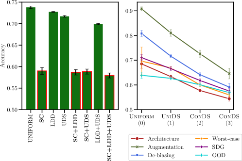
Figure 4: Analysis of model robustness on distribution shifts. Left: Average performance of all generalization methods under different combinations of DSs. Right: Comparing the different generalization methods under an increasing number of DSs.

Table 4: An example of zero-shot inference prompts. The first two rows show the ‘General’ prompts and the next three rows the ‘Tailored’ prompts that we used with LLaVA-1.5. For a more comprehensive list of these prompts, please see Table 12 in Section B.5.

Type	Prompt
General1	USER: <image>
	Classify the image into $label_{1},\dots,$ or $label_{C}$. Please provide only the name of the label.
General2	USER: <image>
	Choose a label that best describes the image. Here is the list of labels to choose from: $label_{1},\dots,label_{C}$.
	Please provide only the name of the label.
dSprites	USER: <image>
Shapes3D	Classify the object in the image into $label_{1},...,$ or $label_{C}$. Please provide only the name of the label.
SmallNorb
CelebA	USER: <image>
	Classify the person in the image into $label_{1}$ or $label_{2}$. Please provide only the name of the label.
DeepFashion	USER: <image>
	Is a person wearing a dress or not? Please answer in yes or no.

Table 5: Comparison of the performance of visual language models across different types of prompts. We report the best results obtained from this ablation study in Figure 3, 8 and Table 3. Note how sensitive the results are to the prompts used. There can be a drop in accuracy of 37% with a suboptimal prompt.

Model	Prompt	dSprites	Shapes3D	SmallNorb	CelebA	DeepFashion	iWildCam	fMoW	Camelyon17
CLIP-base	General	75.19	71.41	72.02	98.5	77.50	13.97	13.30	50.01
CLIP-large	General	90.86	85.39	86.00	97.62	71.25	13.70	23.46	50.01
InstructBLIP	General1	50.25	50.08	26.59	98.63	61.25	1.32	11.61	50.57
	General2	53.46	53.05	36.22	70.50	47.50	1.86	18.17	68.03
	Tailored	58.89	74.77	25.41	78.25	86.25	1.10	9.67	50.00
LLaVA-1.5	General1	49.01	52.89	90.05	98.50	70.00	4.64	15.04	50.57
	General2	72.72	74.61	87.81	98.88	91.25	1.60	16.32	51.09
	Tailored	86.42	71.02	88.16	98.88	88.75	1.85	14.24	50.00
Phi-3.5-vision	General1	88.27	72.73	83.20	98.62	82.50	5.88	9.67	64.86
	General2	88.27	72.50	85.41	98.75	78.75	4.06	10.88	57.09
	Tailored	88.77	72.58	83.30	98.62	53.75	9.91	9.17	66.71
GPT-4o mini	General1	96.79	94.77	81.12	93.87	50.0	43.43	18.87	64.81
	General2	92.84	94.77	78.37	93.87	50.0	43.36	19.28	64.87
	Tailored	92.84	94.77	82.69	93.87	50.0	41.88	19.89	64.98
GPT-4o	General1	92.84	94.77	80.22	82.87	50.00	51.64	24.98	58.02
	General2	92.84	94.77	78.37	93.75	51.25	51.80	24.89	58.03
	Tailored	92.84	94.77	78.85	89.62	50.0	51.21	25.58	58.10

Further analysis on prompts of foundation model.

We investigate various prompts to assess the effectiveness of foundation models for robust image classification. We assess the accuracy of the models in Table 5. For CLIP, we use widely adopted prompts, such as "a photo of a label" (Matsuura et al., ). Given that vision-language models designed for visual question answering may depend on the query’s context, the choice of prompts is crucial (Sahoo et al., 2024). We categorize prompts that are applicable to any dataset as ‘General’, and those specifically designed for each dataset as ‘Tailored’. We provide several examples for the prompt in Table 4. In Matsuura et al. and Islam et al. (2023), diverse prompts are employed as queries for vision-language models, specifically tailored to the dataset and the labels targeted for classification. Our analysis builds on this approach.

5.3 Takeaways

Takeaway 1 – ConDS is, on average, more challenging than UniDS. While previous studies on model generalization have primarily focused on UniDS, we observe that most algorithms exhibit poorer performance in ConDS. Moreover, the more numerous the DSs, the greater the challenge they pose, as illustrated in Figure 4 (right).

Takeaway 2 – SC is the most challenging DS, followed by UDS and LDD. Figure 4 (left) breaks down the performance of generalization methods according to DS. We see that the presence of SC tends to dominate over other DSs in ConDS. Although ConDS presents more challenges than UniDS for LDD and UDS, there is almost no performance drop when moving from SC to SC+LDD or SC+UDS. Furthemore, for the DSs that include SC, the performance of most methods is inferior to that of foundation models even when it is pre-trained, as shown in Figure 8.

Takeaway 3 – Generalization tends to be consistent across DSs. If a method improves generalization for one DS, it tends to be effective for others. Namely, although models such as de-biasing, worst-case generalization, and domain generalization are designed to address a specific DS (as detailed in Section 4), their applicability is not confined to that particular shift.

5.3.1 Takeaways Common to both UniDS and ConDS 

The following takeaways with UniDS have been previously identified by Sahoo et al. (2024); Wiles et al. (2021). We observe that these phenomena persist even in the ConDS scenario.

Takeaway 4 – Heuristic augmentations and pre-training are highly effective. As depicted in Figure 3, heuristic augmentations overall improve the model’s robustness across all DSs. This remains consistent when pre-trained weights are utilized except for ImageNet augmentation (Figure 8 in the supplementary). All the augmentation methods even increase the performance of ResNet18 when used on Uniform, where there is no DS, establishing them as a more effective tool. Algorithms demonstrate improved performance with ImageNet pre-trained weights, as shown in Table 3. On LDD, UDS, and LDD+UDS, most methods even outperform foundation models, as depicted in Figure 8.

Takeaway 5 – Generalization algorithms provide a limited performance improvement. While some methods (L2D, PnD, OccamNets) perform well, most methods exhibit limitations. Existing generalization methods, though competitive in their original experimental setups and benchmarks, demonstrate reduced effectiveness in our more standardized and fair setup.

Takeaway 6 – Foundation pre-trained models are effective, but their performance can vary. Although foundation models demonstrate impressive performance on controlled datasets, they show limited performance compared to other baselines with ImageNet-pretrained weights, as shown in Figure 8. Notably, they exhibit the lowest accuracy on real-world datasets (Table 3). This observation underscores that the performance in image classification significantly depends on the datasets used to train these foundation models, highlighting potential limitations in their applicability. E.g., for specialized datasets like Camelyon17, large models with zero-shot inference can barely make accurate predictions (Table 12). Furthermore, we find that their performances are significantly influenced by the prompt we input (Please refer Table 5 and Table 12 in the Section B.5 for more details).

6 Concluding Remark

Contribution. In this paper, we introduce a novel evaluation framework to understand the robustness of models against various distribution shifts, including UniDS and ConDS. Using this protocol, we can create distribution shifts in any multi-attribute-annotated dataset, allowing for a more comprehensive understanding of robustness. Through our extensive evaluation involving 100K experiments, we find that ConDS present greater challenges compared to conventional UniDS, with spurious correlations being more problematic than low data drift and unseen domain shifts. Our results indicate that heuristic augmentations and pre-training are effective tools for enhancing generalization, while more complex models offer limited benefits. Additionally, while large models are viable for image classification, their performance is effective only in specific scenarios and requires careful application.

Limitation and future work. While we believe that our work makes a promising step towards understanding how models behave under complex scenarios, there is still a lot more that can be done in this direction, we briefly discuss some of them. Our evaluation framework allows us to create controlled distribution shifts and assumes a uniform test distribution. Our framework also uses annotated, thus, interpretable attributes to create shifts. Using learned attributes would also be an interesting future direction. Furthermore, our study covers a limited range of attributes, particularly in controlled real-world datasets such as CelebA and DeepFashion, due to insufficient samples for other attributes. Future research could explore the use of advanced controllable generative models (e.g., diffusion models) to address this limitation and cover a broader range of conditions.

Acknowledgments.

Myeongho Jeon, jointly affiliated with EPFL and Seoul National University, was supported by the National Research Foundation of Korea (NRF) grant funded by the Korea government (MSIT) [RS-2024-00337693]. Suhwan Choi was supported by the Ministry of Culture, Sports and Tourism & Korea Creative Content Agency [RS-2024-00399433], and Artificial intelligence industrial convergence cluster development project funded by the Ministry of Science and ICT (MSIT, Korea) & Gwangju Metropolitan City. We also extend our sincere thanks to CRABs.ai for their generous financial support and the provision of GPU resources.

Appendix A Detailed Experimental Setup

A.1 Setup for Controlled Distribution Shifts

We utilize multi-attribute datasets such as dSprites, Shapes3D, SmallNorb, CelebA, and DeepFashion to develop ConDS. These datasets enable us to sample images annotated with various attributes, showcasing a range of DSs from SC to (SC, LDD, UDS). Additionally, we configure different attributes for each type of DS. For instance, in SC, pairs like ($y^{\alpha}$, $y^{l}$) and ($y^{l}$, $y^{\beta}$) may exhibit spurious correlations. By covering all possible attribute combinations (with the attributes depicted in Figure 5), we ensure a more comprehensive evaluation of scenarios.

For UniDS, we choose one attribute from three options, yielding three settings. In ConDS, we address two combinations: (SC, LDD), (SC, UDS), and (LDD, UDS). For each combination, one attribute is selected for the first DS and another for the second, following a ${}_{3}C_{2}$ selection method. For the three-attribute combination in ConDS, namely (SC, LDD, UDS), one attribute is chosen for the first DS, another for the second, and the remaining for the last DS, in line with a ${}_{3}C_{3}$ approach. With five datasets in a controlled setup, this generates a total of 165 (source, target) pairs.

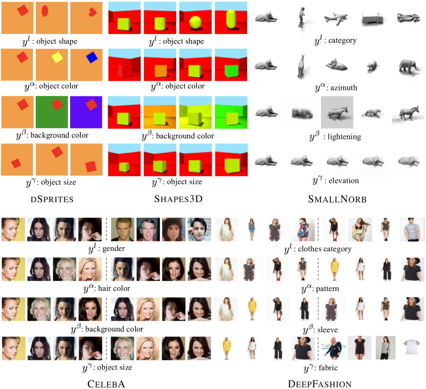
Figure 5: Samples of controlled datasets. We provide visualizations of some samples along with their attributes.

A.2 Dataset Configuration

We provide detailed counts for each split within the datasets. To create the DSs as outlined in Section 3, variations in dataset sizes across the DSs result from the limited availability of certain attribute combinations.

Table 6: Dataset size. Please note that we have included 1% counterexamples for SC in our input.

	dSprites	Shapes3D	SmallNorb	CelebA	DeepFashion
UNIFORM	1,091	65	127	227	97
SC	1,091	65	127	227	97
LDD	1,080	624	1,600	224	112
UDS	1,080	192	500	224	96
SC + LDD	1,091	158	324	227	99
SC + UDS	1,091	49	101	227	101
LDD + UDS	1,080	468	1,280	224	98
SC+ LDD + UDS	1,091	119	259	227	92
TEST	810	1,280	3,125	800	80

Additionally, we detail the method used to introduce distribution shifts in the original datasets as follows:

• dSprites: There are no predefined splits, such as train, validation, or test, in the dSprites dataset; it contains only images and their attribute information. We first created train and test pools by randomly splitting the images, then sampled from each pool to introduce distribution shifts. For the object size attribute, we used the attribute values $[0.8,0.9,1]$, labeling them as small, medium, and large, respectively. Since the original dataset is grayscale, we applied our own colorization: Object colors include red $(255,0,0)$, yellow $(255,255,0)$, and blue $(0,0,255)$, while background colors are set as orange $(255,153,51)$, green $(0,153,0)$, and purple $(102,0,255)$. We allocated 20% of the training set as the validation set for parameter tuning, ensuring that both share the same distribution.

• Shapes3D: There are no predefined splits, such as train, validation, or test, in the Shapes3D dataset; it contains only images and their attribute information. For the object size attribute, we used the attribute values $[0.75,0.964,1.036,1.179]$, labeling them as tiny, small, medium, and large, respectively. We used $[0,0.1,0.2,0.3]$ for object color and $[0,0.1,0.2,0.3]$ for background color. For each unique combination of labels and attributes, we divided the data instances into training and testing sets. We allocated 20% of the training set as the validation set for parameter tuning, ensuring that both share the same distribution.

• SmallNorb: We used the original train-test split provided by SmallNorb, selecting elevations $[0,2,4,6,8]$, azimuths $[0,8,16,24,32]$, and lighting conditions $[0,1,2,3,4]$. To ensure consistency across categories, we manually adjusted the azimuth values for all animal categories, as their initial starting points (0) differed. We allocated 20% of the training set as the validation set for parameter tuning, ensuring that both share the same distribution.

• CelebA: Using all samples in the dataset, we first selected the attributes Black_Hair, Smiling, and Straight_Hair. We then split each combination of these attributes into training and testing sets. The training set was used to create distribution shifts, while all test splits were combined to form a uniform distribution. These three attributes were chosen because they provide sufficient samples to accommodate distribution shifts. We allocated 15% of the training set as the validation set for parameter tuning, ensuring that both share the same distribution.

• DeepFashion: Using all samples in the dataset, we first selected the attributes texture {floral, solid}, shape {mini_length, no_dress}, and style {chiffon, cotton}. We then split each combination of these attributes into training and testing sets. The training set was used to create distribution shifts, while all test splits were combined to form a uniform distribution. These three attributes were chosen because they provide sufficient samples to accommodate distribution shifts. We allocated 20% of the training set as the validation set for parameter tuning, ensuring that both share the same distribution.

A.3 Synthetic and Real-world Datasets

We can precisely manage distribution shifts with synthetic datasets because they allow for complete control. Real-world datasets, on the other hand, offer the advantage of realism but may experience uncontrolled distribution shifts. For instance, suppose we create a gender classifier with a dataset that exhibits a spurious correlation by sampling images of older females and younger males. Despite our efforts, we cannot ensure uniformity across other attributes such as skin tone and gender. Given the advantages and disadvantages of each, we conducted experiments with a variety of synthetic datasets (Dsprites, Shapes3D, Smallnorb) and realistic datasets (CelebA, DeepFashion, iWildCam, fMoW, Camelyon17).

A.4 Benchmarking Methodology

We outline the benchmarking standards in Table 7.

Table 7: Benchmarking Methodology

Aspect	Configuration	Justification
Evaluation Metric	Accuracy: For the controlled dataset, accuracy is used as the evaluation metric since the test set is uniformly distributed, providing a reliable measure of generalization. For iWildS datasets, accuracy follows the setup of the original paper.	Ensures consistent generalization measurement and alignment with benchmark standards.
Image Standardization	Pixel values normalized to a range of (-1, 1).	Stabilizes learning and prevents gradient vanishing.
Learning Stop Criterion	Early stopping applied with a patience of 20 epochs or a maximum of 10,000 iterations. Validation accuracy is measured every 100 iterations; if the highest validation accuracy is not reached, patience decreases by one. Upon achieving the highest validation accuracy, patience resets to 20.	Mitigates overfitting while optimizing model performance.
Image Size	Configured per dataset: 64x64 (dsprites, shapes3d), 96x96 (smallnorb, camelyon17), 128x128 (deepfashion), 224x224 (fmow, iwildcam), and 256x256 (celeba).	We maintain the original image sizes of the datasets.

A.5 Computing Resource

All our experiments were performed using 8 NVIDIA H100 80GB HBM3 GPUs and Intel(R) Xeon(R) Gold 6448Y.

A.6 Implementation Details

To generate all the results reported in this script, we fine-tuned the hyperparameters. For the controlled datasets, we adopt early stopping where training stops early once the patience limit is reached. Validation accuracy is measured every 100 iterations and one patience is consumed if the best validation accuracy does not improve. The specific values are detailed in Table 8 and Table 9. We conducted a grid search with these parameters to optimize results for each algorithm across all DSs and datasets.

Table 8: General Hyperparameters.

Dataset	Learning Rate	Batch Size	Duration	Patience	Optimizer
Controlled	[1e-2, 1e-3, 1e-4]	128	10000 iterations	20	Adam
Real-world	[1e-3, 5e-4, 1e-4, 5e-5, 1e-5]	128	10000 iterations	20	Adam

Table 9: Hyperparameters for specific methods.

Method	Dataset	Hyperparameters
ViT	All	Model: ViT$\_$B$\_$16
MLP	All	$\#$layers: 4, hidden dim: 256
ImageNet	Controlled	scale lower bound: 0.08
	Real-world	scale lower bound: 0.3
AugMix	Controlled	severity: 3, mixture width: 3
	Real-world	severity: 7, mixture width: 5
RandAug	Controlled	num$\_$ops: 3, magnitude: 5
	Real-world	num_ops: 2, magnitude: 9
AutoAug	All	CIFAR10 policy for dSprites, Shapes3D, and SmallNorb.
		Otherwise, ImageNet policy
UBNet	All	base model patience: 10, base model training epochs: 50
PnD	All	$\alpha_{1}$: 0.2, $\alpha_{2}$: 2, $\beta$: 4, $q$: 0.7, $\text{EMA}_{\alpha}$: 0.7,
		base model patience: 10, base model training epochs: 50
OccamNets	All	$\lambda_{CS}$: 0.1, $\lambda_{G}$: 1, $\gamma_{0}$: 3, $\gamma$: 1, $\tau_{acc,0}$: 0.5
	fMoW:	$\tau_{acc,0}$: 0.2
GroupDRO	All	$\lambda$: 1e-2
BPA	All	$k$: 8, $m$: 0.3, base model patience: 10, base model training epochs: 50
	iWildcam	$k$: 12
ADA	All	$T_{max}$: 15, $k$: 2, $\gamma$: 1.0
ME-ADA	All	$T_{max}$: 15, $k$: 2, $\gamma$: 1, $\eta$: 1.0
SagNet	All	$\lambda_{adv}$: 0.1
L2D	All	$\alpha_{1}$: 1, $\alpha_{2}$: 1, $\beta$: 0.1
IRM	All	annealing iterations: 500, $\lambda$: 1 (during annealing), 100 (after annealing)
CausIRL	Controlled	$\gamma$: 0.5 (SmallNorb), 0.3 (dSprites), 0.1 (DeepFashion, CelebA), 1 (Shapes3D)
	Real-world	$\gamma$: 1
CLIP-base	All	model: "openai/clip-vit-base-patch32"
CLIP-Large	All	model: "openai/clip-vit-large-patch14"
InstructBLIP	Inference	model: "Salesforce/instructblip-vicuna-7b",num$\_$beam: 5, load$\_$in$\_$4bit: True
		top$\_$p: 0.9, repetition$\_$penalty: 1.5, length$\_$penalty: 1.0, temperature: 1, max$\_$new$\_$tokens: 20
	Fine-tuning	lora-r: 8
LLaVA-1.5	Inference	model: "llava-hf/llava-1.5-7b-hf", max$\_$new$\_$tokens: 200
	Fine-tuning	lora-r: 128
Phi-3.5-vision	Inference	model: "microsoft/Phi-3.5-vision-instruct", max$\_$new$\_$tokens: 200, temperature: 0.2
	Fine-tuning	lora-r: 64
GPT-4o mini	All	temperature:1, $top_{p}$:1
GPT-4o	All	temperature:1, $top_{p}$:1

Appendix B Experimental Results

B.1 Comprehensive Results

Figure 6 displays the results for all algorithms trained from scratch across all DSs, while Figure 7 presents the outcomes for all algorithms trained using ImageNet pre-trained weights.

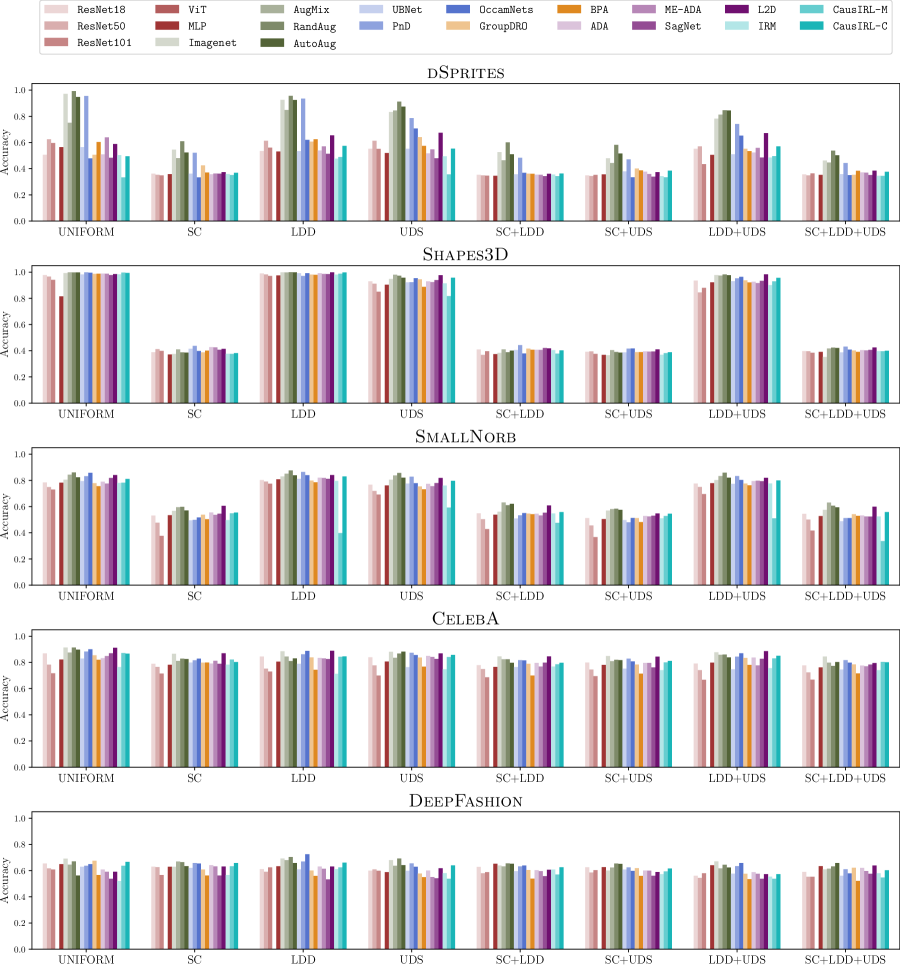
Figure 6: Results for all algorithms from scratch. We plot the top-1 accuracy.

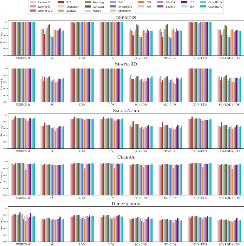
Figure 7: Results for all algorithms with pre-trained weight. We plot the top-1 accuracy.

B.2 Experimental Study on Pre-training

Figure 8 presents the aggregate results of pre-training across all algorithms and DSs.

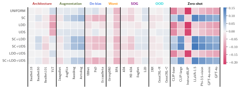
Figure 8: Result with ImageNet pre-trained weight. The setup is the same as Figure 3.

B.3 Analysis across Different Data Sizes

We further analyze the aggregate results across different dataset sizes. As shown in Table 10, we evaluate the algorithms in three variations: small, medium, and large (see from Figure 9 to Figure 20). Although the overall trend remains similar, some differences are observed.

Table 10: Various Dataset size. Please note that we have included 1% counterexamples for SC in our input.

	Shapes3D			CelebA
	small	middle	big	small	middle	big
SC	65	130	194	114	227	340
LDD	624	1,248	1,872	112	224	336
UDS	192	384	576	112	224	336
SC + LDD	158	316	473	114	227	340
SC + UDS	49	97	146	114	227	340
LDD + UDS	468	936	1,404	112	224	336
SC+ LDD + UDS	119	237	355	114	227	340

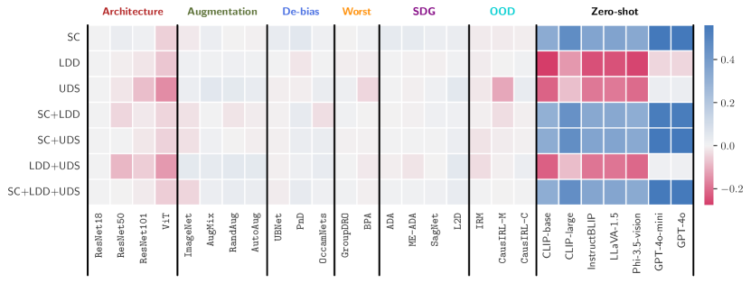
Figure 9: Scratch Shapes3D result with small dataset size. The setup is the same as Figure 3.

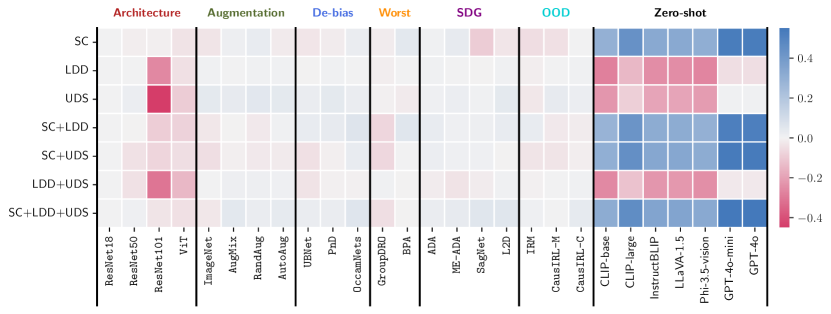
Figure 10: Scratch Shapes3D result with middle dataset size. The setup is the same as Figure 3.

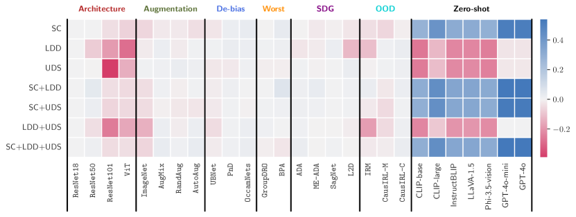
Figure 11: Scratch Shapes3d result with big dataset size. The setup is the same as Figure 3.

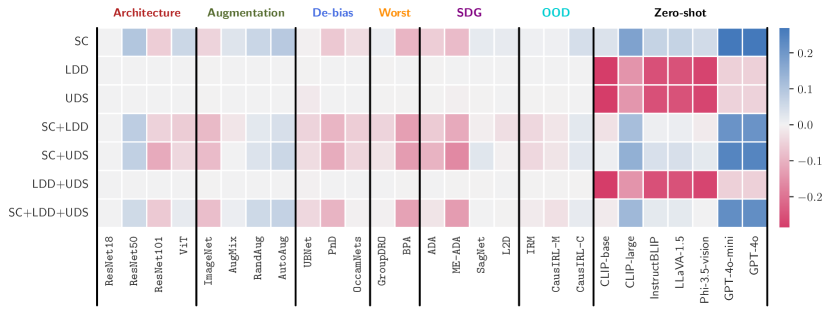
Figure 12: Pretrain Shapes3d result with small dataset size. The setup is the same as Figure 3.

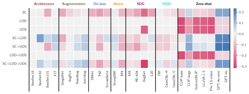
Figure 13: Pretrain Shapes3d result with middle dataset size. The setup is the same as Figure 3.

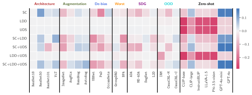
Figure 14: Pretrain Shapes3d result with big dataset size. The setup is the same as Figure 3.

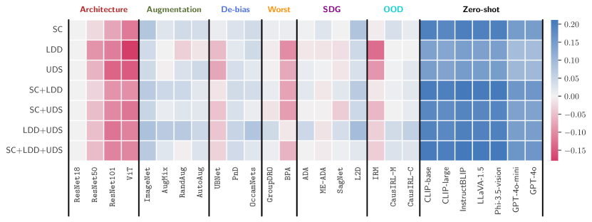
Figure 15: Scratch CelebA result with small dataset size. The setup is the same as Figure 3.

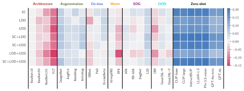
Figure 16: Scratch CelebA result with middle dataset size. The setup is the same as Figure 3.

Figure 17: Scratch CelebA result with big dataset size. The setup is the same as Figure 3.

Figure 18: Pretrain CelebA result with small dataset size. The setup is the same as Figure 3.

Figure 19: Pretrain CelebA result with middle dataset size. The setup is the same as Figure 3.

Figure 20: Pretrain CelebA result with big dataset size. The setup is the same as Figure 3.

B.4 Results for Real-world datasets

Table 11 presents the detailed results for each dataset listed in Table 3.

Table 11: Experimental results on real-world datasets. The setting is exactly the same as Table 3.

		iWildCam		fMoW		Camelyon17
		Scratch	Pre-training	Scratch	Pre-training	Scratch	Pre-training
Architecture	ResNet18	51.77($\pm$0.47)	59.50($\pm$0.43)	27.13($\pm$0.44)	41.08($\pm$0.44)	82.83($\pm$0.25)	84.35($\pm$0.10)
	ResNet50	53.35($\pm$0.34)	66.75($\pm$0.39)	28.55($\pm$0.44)	49.75($\pm$0.32)	75.85($\pm$0.36)	86.78($\pm$0.38)
	ResNet101	43.41($\pm$0.07)	69.71($\pm$0.20)	22.35($\pm$0.30)	48.63($\pm$0.17)	75.26($\pm$0.37)	84.21($\pm$0.49)
	ViT	51.68($\pm$0.33)	69.82($\pm$0.45)	23.20($\pm$0.53)	51.74($\pm$0.46)	76.78($\pm$0.18)	91.27($\pm$0.34)
	avg.	50.05($\pm$2.25)	66.45($\pm$2.42)	25.31($\pm$1.50)	47.80($\pm$2.33)	77.68($\pm$1.74)	86.65($\pm$1.65)
Augmentation	Imagenet	48.21($\pm$0.21)	64.17($\pm$0.39)	26.16($\pm$0.53)	47.32($\pm$0.33)	72.08($\pm$0.34)	87.95($\pm$0.39)
	AugMix	51.90($\pm$0.29)	65.61($\pm$0.43)	29.94($\pm$0.27)	49.95($\pm$0.21)	74.13($\pm$0.41)	88.72($\pm$0.49)
	RandAug	47.49($\pm$0.28)	65.14($\pm$0.05)	31.12($\pm$0.24)	49.48($\pm$0.48)	77.21($\pm$0.41)	90.24($\pm$0.40)
	AutoAug	51.57($\pm$0.32)	70.19($\pm$0.03)	31.64($\pm$0.44)	50.13($\pm$0.24)	73.23($\pm$0.28)	90.56($\pm$0.47)
	avg.	49.79($\pm$1.13)	66.28($\pm$1.34)	29.71($\pm$1.24)	49.22($\pm$0.65)	74.16($\pm$1.10)	89.37($\pm$0.62)
De-biasing	UBNet	32.96($\pm$0.47)	57.96($\pm$0.39)	16.30($\pm$0.48)	37.06($\pm$0.51)	73.77($\pm$0.38)	82.06($\pm$0.12)
	PnD	45.25($\pm$0.42)	61.03($\pm$0.48)	21.01($\pm$0.54)	40.29($\pm$0.40)	83.81($\pm$0.40)	79.69($\pm$0.28)
	OccamNets	53.67($\pm$0.49)	67.30($\pm$0.45)	29.08($\pm$0.27)	46.53($\pm$0.39)	74.97($\pm$0.32)	81.77($\pm$0.47)
	avg.	43.96($\pm$6.01)	62.10($\pm$2.75)	22.13($\pm$3.73)	41.29($\pm$2.78)	77.52($\pm$3.17)	81.17($\pm$0.75)
Worst-case	GroupDRO	45.15($\pm$0.22)	63.15($\pm$0.23)	25.99($\pm$0.46)	49.07($\pm$0.44)	73.37($\pm$0.38)	80.99($\pm$0.35)
	BPA	35.54($\pm$0.23)	56.06($\pm$0.18)	8.71($\pm$0.26)	44.32($\pm$0.17)	76.99($\pm$0.27)	86.08($\pm$0.14)
	avg.	40.35($\pm$4.85)	59.60($\pm$3.54)	17.35($\pm$8.64)	46.70($\pm$2.38)	75.18($\pm$1.81)	83.53($\pm$2.55)
SDG	ADA	48.47($\pm$0.41)	69.99($\pm$0.45)	29.71($\pm$0.36)	50.40($\pm$0.41)	80.45($\pm$0.20)	88.74($\pm$0.25)
	ME-ADA	52.62($\pm$0.26)	65.87($\pm$0.40)	28.46($\pm$0.33)	51.43($\pm$0.35)	80.29($\pm$0.19)	81.93($\pm$0.03)
	SagNet	54.67($\pm$0.50)	69.83($\pm$0.38)	29.53($\pm$0.33)	49.32($\pm$0.32)	78.62($\pm$0.39)	81.10($\pm$0.45)
	L2D	47.78($\pm$0.16)	64.09($\pm$0.49)	23.90($\pm$0.30)	45.65($\pm$0.34)	86.32($\pm$0.23)	94.85($\pm$0.27)
	avg.	50.88($\pm$1.65)	67.44($\pm$1.47)	27.90($\pm$1.36)	49.20($\pm$1.26)	81.42($\pm$1.68)	86.66($\pm$3.22)
OOD	IRM	34.55($\pm$0.51)	57.36($\pm$0.31)	11.40($\pm$0.51)	30.88($\pm$0.36)	72.47($\pm$0.35)	85.45($\pm$0.41)
	CausIRL-M	52.28($\pm$0.50)	68.34($\pm$0.45)	22.32($\pm$0.28)	49.44($\pm$0.11)	72.10($\pm$0.26)	79.83($\pm$0.14)
	CausIRL-C	53.36($\pm$0.40)	65.36($\pm$0.47)	28.61($\pm$0.18)	49.83($\pm$0.13)	81.16($\pm$0.21)	88.98($\pm$0.37)
	avg.	46.73($\pm$6.10)	63.69($\pm$3.28)	20.78($\pm$5.03)	43.38($\pm$6.25)	75.24($\pm$2.96)	84.75($\pm$2.66)
Zero-shot	CLIP-base	13.97		13.30		50.01
	CLIP-large	13.70		23.46		50.01
	InstructBLIP	1.86		18.17		68.03
	LLaVA-1.5	4.64		16.32		51.09
	Phi-3.5-vision	9.91		10.88		66.71
	GPT-4o mini	43.36		19.89		64.98
	GPT-4o	51.80		25.58		58.10
	avg.	19.89		18.23		58.42

B.5 Further Analysis on Zero-shot Inference

To utilize foundation models for image classification, we employed various prompts to extract labels from the input images. Table 12 and Table 13 detail the prompts used in our prompt engineering approach.

Table 12: Prompts used in Zero-shot inference.

Foundation Model	Prompt Type	Prompt
CLIP	General	“a photo of a $label$”
	General1	Classify the image into $label_{1},...,$ or $label_{C}$. Please provide only the name of the label.
	General2	Choose a label that best describes the image. Here is the list of labels to choose from: $label_{1},...,label_{C}$.
		Please provide only the name of the label.
	dSprites
	Shapes3D	Classify the object in the image into $label_{1},...,$ or $label_{C}$. Please provide only the name of the label.
	SmallNorb
LLaVA-1.5	CelebA	Classify the person in the image into $male$ or $female$. Please provide only the name of the label.
InstructBLIP	DeepFashion	Is a person wearing a dress or not? Please answer in yes or no.
Phi-3.5-vision	iWildcam	Classify the object or animal in the image. Here is the list of labels to choose from: $label_{1},...,label_{C}$.
GPT-4o mini		Please provide only the name of the label.
GPT-4o	fMoW	Classify the building or land-use in the image into $label_{1},...,label_{C}$.
		Please provide only the name of the label.
	Camelyon17	Please answer yes if the image contains any tumor tissue, and no otherwise.
	General1	Please provide only the name of the label.
	Camelyon17	Please answer yes if the image contains any tumor tissue, and no otherwise.
	General2	Please respond with a single word.
	Camelyon17	Please analyze the image and determine if it contains any tumor tissue.
	Tailored	Respond with ’Yes’ if tumor tissue is present, or ’No’ if it is not.

Table 13: Prompt formats for vision-language models.

	LLaVA-1.5, InstructBLIP	Phi-3.5-vision	GPT-4o, GPT-4o-mini
Prompt Format	USER: $<$ image $>$\n prompt \n ASSISTANT:	USER: $<|$image_1$|>$\n prompt	prompt

B.6 Fine-tuned Open Source Foundation Model

We observe in Table 3 that the zero-shot performance of foundation models is constrained when applied to real-world datasets. Our evaluation on real-world datasets like Camelyon17, which contains complex cell images, iWildCam with its camera trap images of diverse animal species, and FMoW’s satellite images present unique challenges due to their niche content and visual complexity. This high level of domain specificity, with features likely outside the foundation models’ general scope, limits their capacity to generalize effectively, particularly in zero-shot settings.

An intuitive approach to evaluate this is by fine-tuning the vision encoder on these specialized datasets. Through fine-tuning with LoRA Hu et al. (2022), we found that the foundation models performed as expected, showing high effectiveness for these datasets. The results are presented in Table 14.

Table 14: Fine-tuned open source foundation model. w and w/o denote with and without fine-tuning, respectively.

	iWildCam		Camelyon17		FMoW
	w/o	w	w/o	w	w/o	w
LLaVA-1.5	4.64	91.12	51.09	95.32	16.32	72.67
Phi-3.5-Vision	9.91	91.19	66.71	93.35	10.88	77.02
InstructBLIP	1.86	12.13	68.03	99.87	18.17	41.18

B.7 Visualization on Invariant Feature Learning.

We investigate feature invariance with respect to labels and attributes using the CelebA dataset. UMAP (McInnes et al., 2018) is utilized for visualization. Figure 21 illustrates the feature space of the best and worst-performing algorithms, while Figure 22 compares learning from scratch with pre-training. While all the algorithms demonstrate invariance to LDD and UDS, ViT exhibits sensitivity to SC. In contrast, both CLIP-Large and ImageNet remain invariant to all DSs. In Figure 22, the ViT model with pre-training exhibits better invariance to attributes compared to the ViT model trained from scratch.

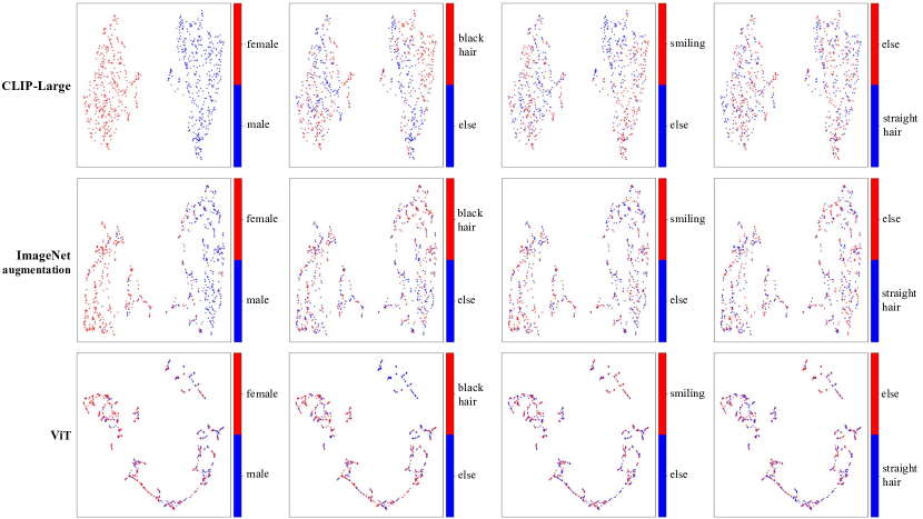
Figure 21: Visualization on invariant feature learning. We visualize the top two algorithms, CLIP-Large and ImageNet, along with the worst-performing algorithm. In this setup, ‘black hair’ is used to create SC, ‘smiling’ is used to generate LDD, and ‘straight hair’ is used to produce UDS.

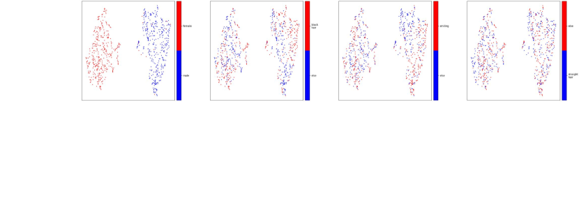
Figure 22: Scratch vs. Pre-training. The setup is exactly the same as Figure 21.

B.8 Generation of Attributes with Augmentations

Our framework requires datasets with rich attribute annotations to create ConDS. However, such datasets are limited as annotations are expensive. We did consider using augmentations to create additional attributions, but augmentation techniques in algorithm baselines might directly address these shifts in this setting. However, for the rebuttal, we applied three types of corruptions from ImageNet-C (Hendrycks & Dietterich, 2018)—impulse noise, snow, and elastic transform—on CelebA. Each attribute was evaluated under two conditions (corrupted and uncorrupted). Figures 23 and 24 exhibit the evaluation results with this setup.

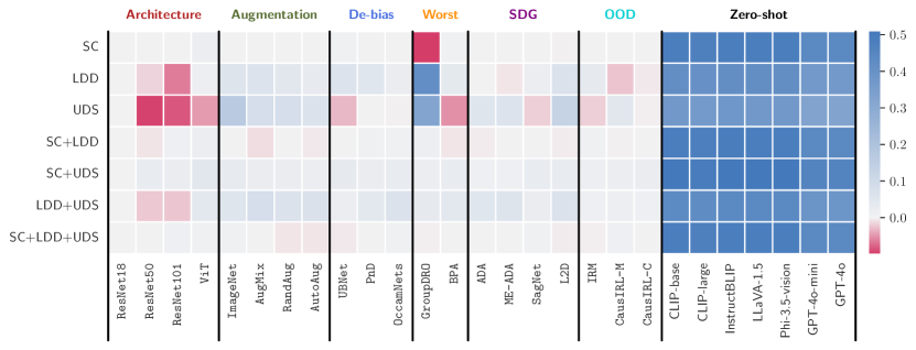
Figure 23: Scratch CelebA result with attributes generated from augmentation. The setup is the same as Figure 3.

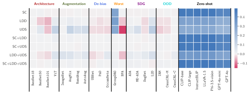
Figure 24: Pretrain CelebA result with attributes generated from augmentation. The setup is the same as Figure 3.

B.9 Results for Distribution Shift Generated by Clustering

We leverage DINOv2 (Oquab et al., 2024) to extract rich image features, using the resulting feature clusters as proxies for DSs. The motivation behind this approach aligns with that of Section B.8, namely, the necessity for a scalable method to simulate DSs without depending on costly and labor-intensive attribute annotations. As displayed in Table 15, we group image features into six clusters based on their embeddings from DINOv2 and treat these clusters as distinct distributions. Figures 25 and 26 exhibit the evaluation results with this setup.

Table 15: Cluster groups. From six clusters, we create four distribution shift groups and one test group, simulating different environmental or contextual variations.

	Group 1	Group 2	Group 3	Group 4	Test
Cluster	1, 4	2, 4	1, 5	2, 5	3, 6

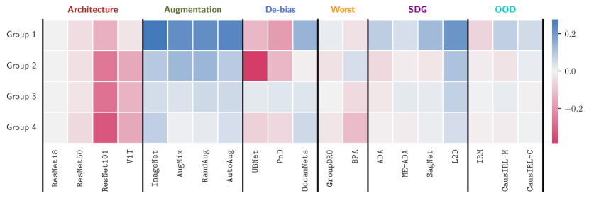
Figure 25: Scratch CelebA results across cluster groups. The setup is the same as Figure 3.

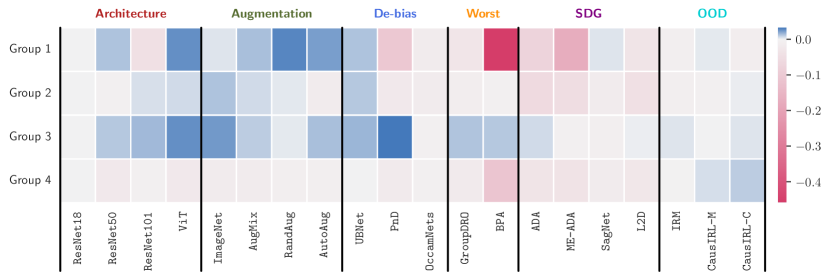
Figure 26: Pretrain CelebA result across cluster groups. The setup is the same as Figure 3.

B.10 Performance Sensitivity for Hyperparameters

We evaluate the performance sensitivity of the algorithms across all datasets and compute the average results. For detailed hyperparameter configurations, please refer to Table 8. Figures 27 - 40 illustrate the results.

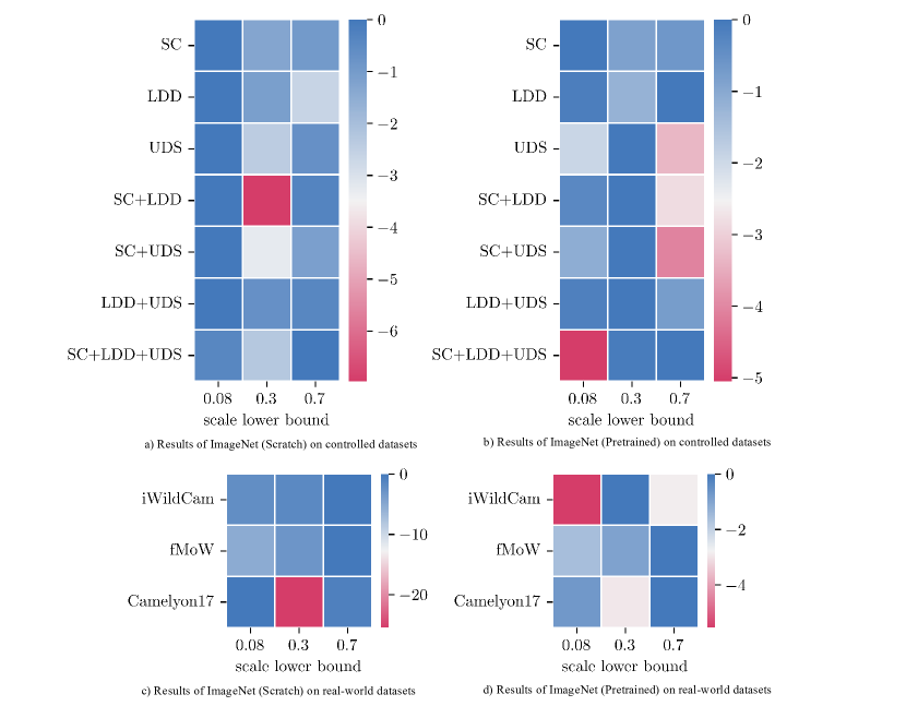
Figure 27: Hyperparameter Exploration for ImageNet.

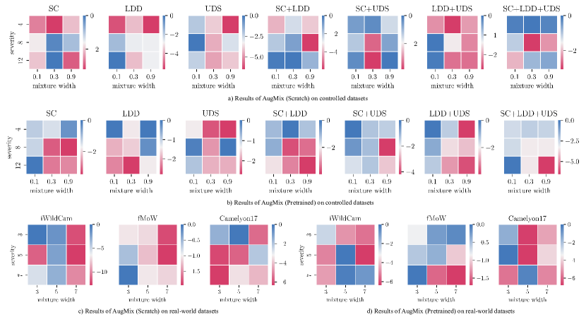
Figure 28: Hyperparameter Exploration for AugMix.

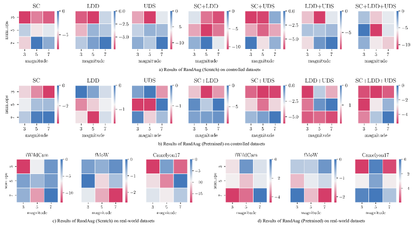
Figure 29: Hyperparameter Exploration for RandAug.

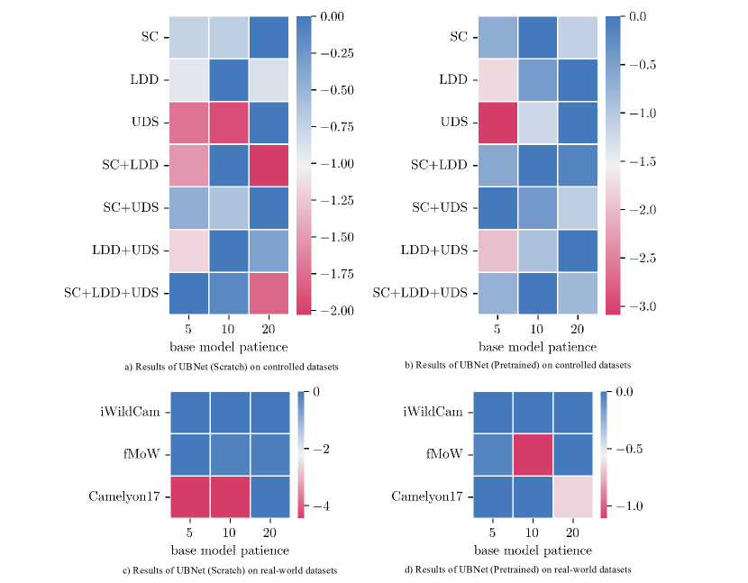
Figure 30: Hyperparameter Exploration for UBNet.

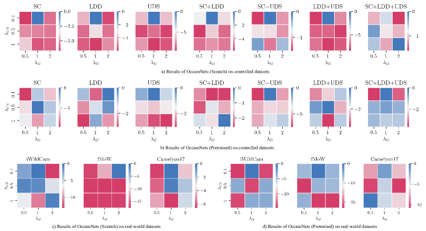
Figure 31: Hyperparameter Exploration for OccamNets.

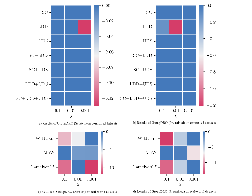
Figure 32: Hyperparameter Exploration for groupDRO.

Figure 33: Hyperparameter Exploration for BPA.

Figure 34: Hyperparameter Exploration for ADA.

Figure 35: Hyperparameter Exploration for ME-ADA.

Figure 36: Hyperparameter Exploration for SagNet.

Figure 37: Hyperparameter Exploration for L2D.

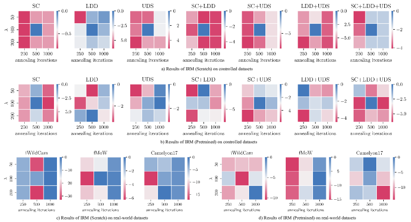
Figure 38: Hyperparameter Exploration for IRM.

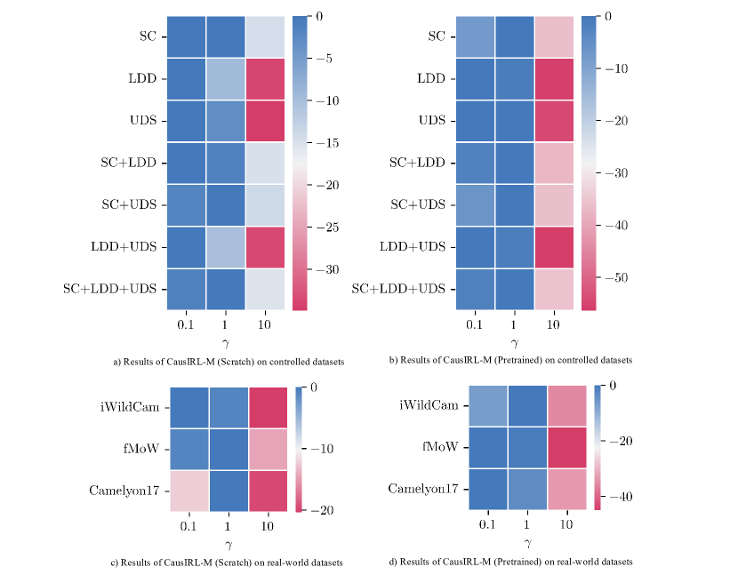
Figure 39: Hyperparameter Exploration for CausIRL-M.

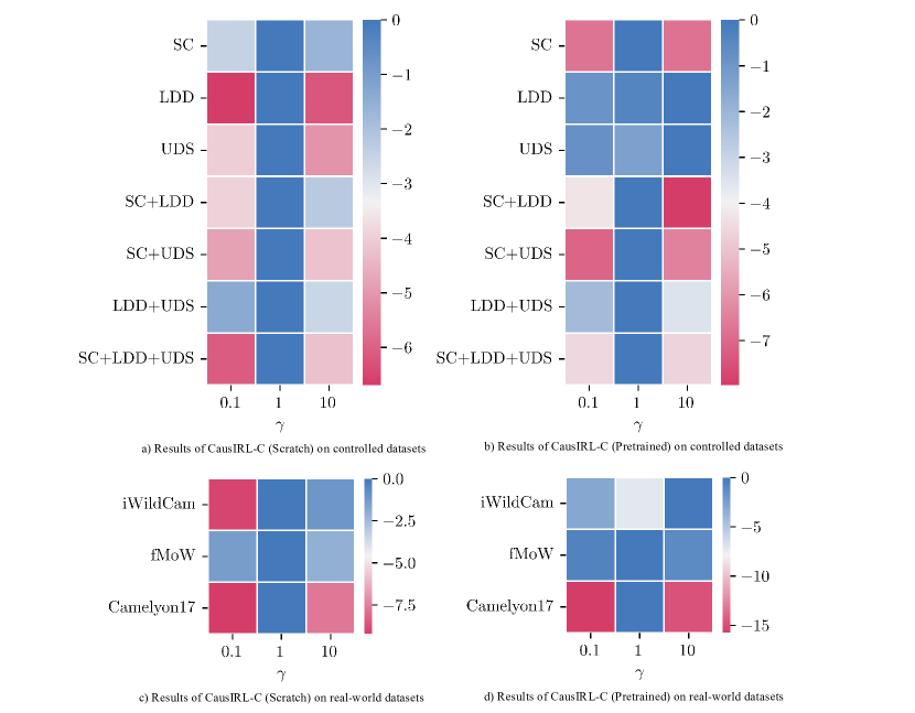
Figure 40: Hyperparameter Exploration for CausIRL-C.

B.11 Computaional Cost

We provide the time and memory costs for all the algorithms, using iWildCam as the dataset for this analysis. Table 16 shows the results.

Category	Method	Time (seconds per epoch)	Memory (MiB)
Architecture	ResNet18	1275	3274
	ResNet50	1270	11640
	ResNet101	1289	17179
	ViT	1258	17844
Augmentation	ImageNet	1405	11640
	AugMix	1617	11640
	RandAug	1418	11640
	AutoAug	1357	11640
SDG	ADA	1301	11487
	ME-ADA	1305	11487
	SagNet	1281	11718
	L2D	1607	24393
OOD	IRM	1272	11640
	CausIRL-MMD	1275	11563
	CausIRL-CORAL	1286	11606
De-bias	UBNet	1262	11489
	PnD	1658	62225
	OccamNets	3218	14669
Worst-case	GroupDRO	1258	11562
	BPA	1249	12235
LVLM (LoRA)	InstructBLIP	50	70567
	LLaVA-1.5	308	110880*
	Phi-3.5-vision	577	12623

Table 16: Performance comparison of different methods across categories, showing time (in seconds) and memory usage (in MiB). Training was performed with a batch size of 128 on a single H100 GPU. LVLM models are fine-tuned using LoRA for Table 14. For LLaVA-1.5, due to memory constraints on a single H100, multi-GPU training was used with two H100s, each handling a batch size of 64, and the total memory usage was combined.

References

- Abdin et al. (2024) Marah Abdin, Sam Ade Jacobs, Ammar Ahmad Awan, Jyoti Aneja, Ahmed Awadallah, Hany Awadalla, Nguyen Bach, Amit Bahree, Arash Bakhtiari, Harkirat Behl, et al. Phi-3 technical report: A highly capable language model locally on your phone. arXiv preprint arXiv:2404.14219, 2024.
- Adeli et al. (2021) Ehsan Adeli, Qingyu Zhao, Adolf Pfefferbaum, Edith V Sullivan, Li Fei-Fei, Juan Carlos Niebles, and Kilian M Pohl. Representation learning with statistical independence to mitigate bias. In Proceedings of the IEEE/CVF Winter Conference on Applications of Computer Vision, pp. 2513–2523, 2021.
- Alvi et al. (2018) Mohsan Alvi, Andrew Zisserman, and Christoffer Nellåker. Turning a blind eye: Explicit removal of biases and variation from deep neural network embeddings. In Proceedings of the European Conference on Computer Vision (ECCV) Workshops, pp. 0–0, 2018.
- Arjovsky et al. (2019) Martin Arjovsky, Léon Bottou, Ishaan Gulrajani, and David Lopez-Paz. Invariant risk minimization. arXiv preprint arXiv:1907.02893, 2019.
- Atanov et al. (2022) Andrei Atanov, Andrei Filatov, Teresa Yeo, Ajay Sohmshetty, and Amir Zamir. Task discovery: Finding the tasks that neural networks generalize on. Advances in Neural Information Processing Systems, 35:15702–15717, 2022.
- Bahng et al. (2020) Hyojin Bahng, Sanghyuk Chun, Sangdoo Yun, Jaegul Choo, and Seong Joon Oh. Learning de-biased representations with biased representations. In International Conference on Machine Learning, pp. 528–539. PMLR, 2020.
- Barbu et al. (2019) Andrei Barbu, David Mayo, Julian Alverio, William Luo, Christopher Wang, Dan Gutfreund, Josh Tenenbaum, and Boris Katz. Objectnet: A large-scale bias-controlled dataset for pushing the limits of object recognition models. Advances in neural information processing systems, 32, 2019.
- Chen et al. (2022) Xi Chen, Xiao Wang, Soravit Changpinyo, AJ Piergiovanni, Piotr Padlewski, Daniel Salz, Sebastian Goodman, Adam Grycner, Basil Mustafa, Lucas Beyer, et al. Pali: A jointly-scaled multilingual language-image model. arXiv preprint arXiv:2209.06794, 2022.
- Chevalley et al. (2022) Mathieu Chevalley, Charlotte Bunne, Andreas Krause, and Stefan Bauer. Invariant causal mechanisms through distribution matching. arXiv preprint arXiv:2206.11646, 2022.
- Cubuk et al. (2019) Ekin D Cubuk, Barret Zoph, Dandelion Mane, Vijay Vasudevan, and Quoc V Le. Autoaugment: Learning augmentation strategies from data. In Proceedings of the IEEE/CVF conference on computer vision and pattern recognition, pp. 113–123, 2019.
- Cubuk et al. (2020) Ekin D Cubuk, Barret Zoph, Jonathon Shlens, and Quoc V Le. Randaugment: Practical automated data augmentation with a reduced search space. In Proceedings of the IEEE/CVF conference on computer vision and pattern recognition workshops, pp. 702–703, 2020.
- Cugu et al. (2022) Ilke Cugu, Massimiliano Mancini, Yanbei Chen, and Zeynep Akata. Attention consistency on visual corruptions for single-source domain generalization. In Proceedings of the IEEE/CVF Conference on Computer Vision and Pattern Recognition, pp. 4165–4174, 2022.
- Dai et al. (2024) Wenliang Dai, Junnan Li, Dongxu Li, Anthony Meng Huat Tiong, Junqi Zhao, Weisheng Wang, Boyang Li, Pascale N Fung, and Steven Hoi. Instructblip: Towards general-purpose vision-language models with instruction tuning. Advances in Neural Information Processing Systems, 36, 2024.
- Dosovitskiy et al. (2020) Alexey Dosovitskiy, Lucas Beyer, Alexander Kolesnikov, Dirk Weissenborn, Xiaohua Zhai, Thomas Unterthiner, Mostafa Dehghani, Matthias Minderer, Georg Heigold, Sylvain Gelly, et al. An image is worth 16x16 words: Transformers for image recognition at scale. arXiv preprint arXiv:2010.11929, 2020.
- Ganin et al. (2016) Yaroslav Ganin, Evgeniya Ustinova, Hana Ajakan, Pascal Germain, Hugo Larochelle, François Laviolette, Mario March, and Victor Lempitsky. Domain-adversarial training of neural networks. Journal of machine learning research, 17(59):1–35, 2016.
- Geirhos et al. (2018) Robert Geirhos, Patricia Rubisch, Claudio Michaelis, Matthias Bethge, Felix A Wichmann, and Wieland Brendel. Imagenet-trained cnns are biased towards texture; increasing shape bias improves accuracy and robustness. arXiv preprint arXiv:1811.12231, 2018.
- Gulrajani & Lopez-Paz (2020) Ishaan Gulrajani and David Lopez-Paz. In search of lost domain generalization. arXiv preprint arXiv:2007.01434, 2020.
- He et al. (2016) Kaiming He, Xiangyu Zhang, Shaoqing Ren, and Jian Sun. Deep residual learning for image recognition. In Proceedings of the IEEE conference on computer vision and pattern recognition, pp. 770–778, 2016.
- Hendrycks & Dietterich (2018) Dan Hendrycks and Thomas Dietterich. Benchmarking neural network robustness to common corruptions and perturbations. In International Conference on Learning Representations, 2018.
- Hendrycks & Dietterich (2019) Dan Hendrycks and Thomas Dietterich. Benchmarking neural network robustness to common corruptions and perturbations. arXiv preprint arXiv:1903.12261, 2019.
- Hendrycks et al. (2019) Dan Hendrycks, Norman Mu, Ekin D Cubuk, Barret Zoph, Justin Gilmer, and Balaji Lakshminarayanan. Augmix: A simple data processing method to improve robustness and uncertainty. arXiv preprint arXiv:1912.02781, 2019.
- Hendrycks et al. (2021) Dan Hendrycks, Steven Basart, Norman Mu, Saurav Kadavath, Frank Wang, Evan Dorundo, Rahul Desai, Tyler Zhu, Samyak Parajuli, Mike Guo, et al. The many faces of robustness: A critical analysis of out-of-distribution generalization. In Proceedings of the IEEE/CVF international conference on computer vision, pp. 8340–8349, 2021.
- Hu et al. (2022) Edward J Hu, Yelong Shen, Phillip Wallis, Zeyuan Allen-Zhu, Yuanzhi Li, Shean Wang, Lu Wang, and Weizhu Chen. LoRA: Low-rank adaptation of large language models. In International Conference on Learning Representations, 2022. URL https://openreview.net/forum?id=nZeVKeeFYf9.
- Islam et al. (2023) Ashhadul Islam, Md Rafiul Biswas, Wajdi Zaghouani, Samir Brahim Belhaouari, and Zubair Shah. Pushing boundaries: Exploring zero shot object classification with large multimodal models. In 2023 Tenth International Conference on Social Networks Analysis, Management and Security (SNAMS), pp. 1–5. IEEE, 2023.
- Jeon et al. (2022a) Myeongho Jeon, Daekyung Kim, Woochul Lee, Myungjoo Kang, and Joonseok Lee. A conservative approach for unbiased learning on unknown biases. In Proceedings of the IEEE/CVF Conference on Computer Vision and Pattern Recognition, pp. 16752–16760, 2022a.
- Jeon et al. (2022b) Myeongho Jeon, Hyoje Lee, Yedarm Seong, and Myungjoo Kang. Learning without prejudices: continual unbiased learning via benign and malignant forgetting. In The Eleventh International Conference on Learning Representations, 2022b.
- Jeon et al. (2023) Myeongho Jeon, Myungjoo Kang, and Joonseok Lee. A unified framework for robustness on diverse sampling errors. In Proceedings of the IEEE/CVF International Conference on Computer Vision, pp. 1464–1472, 2023.
- Karras et al. (2017) Tero Karras, Timo Aila, Samuli Laine, and Jaakko Lehtinen. Progressive growing of gans for improved quality, stability, and variation. arXiv preprint arXiv:1710.10196, 2017.
- Karras et al. (2019) Tero Karras, Samuli Laine, and Timo Aila. A style-based generator architecture for generative adversarial networks. In Proceedings of the IEEE/CVF conference on computer vision and pattern recognition, pp. 4401–4410, 2019.
- Kim et al. (2019) Byungju Kim, Hyunwoo Kim, Kyungsu Kim, Sungjin Kim, and Junmo Kim. Learning not to learn: Training deep neural networks with biased data. In Proceedings of the IEEE/CVF conference on computer vision and pattern recognition, pp. 9012–9020, 2019.
- Koh et al. (2021) Pang Wei Koh, Shiori Sagawa, Henrik Marklund, Sang Michael Xie, Marvin Zhang, Akshay Balsubramani, Weihua Hu, Michihiro Yasunaga, Richard Lanas Phillips, Irena Gao, et al. Wilds: A benchmark of in-the-wild distribution shifts. In International conference on machine learning, pp. 5637–5664. PMLR, 2021.
- Leclerc et al. (2022) Guillaume Leclerc, Hadi Salman, Andrew Ilyas, Sai Vemprala, Logan Engstrom, Vibhav Vineet, Kai Xiao, Pengchuan Zhang, Shibani Santurkar, Greg Yang, et al. 3db: A framework for debugging computer vision models. Advances in Neural Information Processing Systems, 35:8498–8511, 2022.
- Lee et al. (2021) Jungsoo Lee, Eungyeup Kim, Juyoung Lee, Jihyeon Lee, and Jaegul Choo. Learning debiased representation via disentangled feature augmentation. Advances in Neural Information Processing Systems, 34:25123–25133, 2021.
- Li et al. (2017) Da Li, Yongxin Yang, Yi-Zhe Song, and Timothy M Hospedales. Deeper, broader and artier domain generalization. In Proceedings of the IEEE international conference on computer vision, pp. 5542–5550, 2017.
- Li et al. (2023) Jiaxuan Li, Duc Minh Vo, and Hideki Nakayama. Partition-and-debias: Agnostic biases mitigation via a mixture of biases-specific experts. In Proceedings of the IEEE/CVF International Conference on Computer Vision, pp. 4924–4934, 2023.
- Liu et al. (2023) Haotian Liu, Chunyuan Li, Yuheng Li, and Yong Jae Lee. Improved baselines with visual instruction tuning. arXiv preprint arXiv:2310.03744, 2023.
- (37) Misaki Matsuura, Young Kyun Jung, and Ser Nam Lim. Visual-llm zero-shot classification.
- McInnes et al. (2018) Leland McInnes, John Healy, and James Melville. Umap: Uniform manifold approximation and projection for dimension reduction. arXiv preprint arXiv:1802.03426, 2018.
- Miller et al. (2021) John P Miller, Rohan Taori, Aditi Raghunathan, Shiori Sagawa, Pang Wei Koh, Vaishaal Shankar, Percy Liang, Yair Carmon, and Ludwig Schmidt. Accuracy on the line: on the strong correlation between out-of-distribution and in-distribution generalization. In International conference on machine learning, pp. 7721–7735. PMLR, 2021.
- Nam et al. (2021) Hyeonseob Nam, HyunJae Lee, Jongchan Park, Wonjun Yoon, and Donggeun Yoo. Reducing domain gap by reducing style bias. In Proceedings of the IEEE/CVF Conference on Computer Vision and Pattern Recognition, pp. 8690–8699, 2021.
- Nam et al. (2020) Junhyun Nam, Hyuntak Cha, Sungsoo Ahn, Jaeho Lee, and Jinwoo Shin. Learning from failure: De-biasing classifier from biased classifier. Advances in Neural Information Processing Systems, 33:20673–20684, 2020.
- OpenAI (2024) OpenAI. Hello gpt-4o. https://openai.com/index/hello-gpt-4o/, 2024. Accessed: 2024-05-26.
- Oquab et al. (2024) Maxime Oquab, Timothée Darcet, Théo Moutakanni, Huy Vo, Marc Szafraniec, Vasil Khalidov, Pierre Fernandez, Daniel Haziza, Francisco Massa, Alaaeldin El-Nouby, Mahmoud Assran, Nicolas Ballas, Wojciech Galuba, Russell Howes, Po-Yao Huang, Shang-Wen Li, Ishan Misra, Michael Rabbat, Vasu Sharma, Gabriel Synnaeve, Hu Xu, Hervé Jegou, Julien Mairal, Patrick Labatut, Armand Joulin, and Piotr Bojanowski. Dinov2: Learning robust visual features without supervision, 2024.
- Peng et al. (2019) Xingchao Peng, Qinxun Bai, Xide Xia, Zijun Huang, Kate Saenko, and Bo Wang. Moment matching for multi-source domain adaptation. In Proceedings of the IEEE/CVF international conference on computer vision, pp. 1406–1415, 2019.
- Radford et al. (2021) Alec Radford, Jong Wook Kim, Chris Hallacy, Aditya Ramesh, Gabriel Goh, Sandhini Agarwal, Girish Sastry, Amanda Askell, Pamela Mishkin, Jack Clark, et al. Learning transferable visual models from natural language supervision. In International conference on machine learning, pp. 8748–8763. PMLR, 2021.
- Recht et al. (2019) Benjamin Recht, Rebecca Roelofs, Ludwig Schmidt, and Vaishaal Shankar. Do imagenet classifiers generalize to imagenet? In International conference on machine learning, pp. 5389–5400. PMLR, 2019.
- Sagawa et al. (2019) Shiori Sagawa, Pang Wei Koh, Tatsunori B Hashimoto, and Percy Liang. Distributionally robust neural networks for group shifts: On the importance of regularization for worst-case generalization. arXiv preprint arXiv:1911.08731, 2019.
- Sahoo et al. (2024) Pranab Sahoo, Ayush Kumar Singh, Sriparna Saha, Vinija Jain, Samrat Mondal, and Aman Chadha. A systematic survey of prompt engineering in large language models: Techniques and applications. arXiv preprint arXiv:2402.07927, 2024.
- Seo et al. (2022) Seonguk Seo, Joon-Young Lee, and Bohyung Han. Unsupervised learning of debiased representations with pseudo-attributes. In Proceedings of the IEEE/CVF Conference on Computer Vision and Pattern Recognition, pp. 16742–16751, 2022.
- Shrestha et al. (2022) Robik Shrestha, Kushal Kafle, and Christopher Kanan. Occamnets: Mitigating dataset bias by favoring simpler hypotheses. In European Conference on Computer Vision, pp. 702–721. Springer, 2022.
- Sun et al. (2022) Tao Sun, Mattia Segu, Janis Postels, Yuxuan Wang, Luc Van Gool, Bernt Schiele, Federico Tombari, and Fisher Yu. Shift: a synthetic driving dataset for continuous multi-task domain adaptation. In Proceedings of the IEEE/CVF Conference on Computer Vision and Pattern Recognition, pp. 21371–21382, 2022.
- Taori et al. (2020) Rohan Taori, Achal Dave, Vaishaal Shankar, Nicholas Carlini, Benjamin Recht, and Ludwig Schmidt. Measuring robustness to natural distribution shifts in image classification. Advances in Neural Information Processing Systems, 33:18583–18599, 2020.
- Vapnik (1991) Vladimir Vapnik. Principles of risk minimization for learning theory. Advances in neural information processing systems, 4, 1991.
- Venkateswara et al. (2017) Hemanth Venkateswara, Jose Eusebio, Shayok Chakraborty, and Sethuraman Panchanathan. Deep hashing network for unsupervised domain adaptation. In Proceedings of the IEEE conference on computer vision and pattern recognition, pp. 5018–5027, 2017.
- Volpi et al. (2018) Riccardo Volpi, Hongseok Namkoong, Ozan Sener, John C Duchi, Vittorio Murino, and Silvio Savarese. Generalizing to unseen domains via adversarial data augmentation. Advances in neural information processing systems, 31, 2018.
- Wang et al. (2021) Zijian Wang, Yadan Luo, Ruihong Qiu, Zi Huang, and Mahsa Baktashmotlagh. Learning to diversify for single domain generalization. In Proceedings of the IEEE/CVF International Conference on Computer Vision, pp. 834–843, 2021.
- Wenzel et al. (2022) Florian Wenzel, Andrea Dittadi, Peter Gehler, Carl-Johann Simon-Gabriel, Max Horn, Dominik Zietlow, David Kernert, Chris Russell, Thomas Brox, Bernt Schiele, et al. Assaying out-of-distribution generalization in transfer learning. Advances in Neural Information Processing Systems, 35:7181–7198, 2022.
- Wiles et al. (2021) Olivia Wiles, Sven Gowal, Florian Stimberg, Sylvestre Alvise-Rebuffi, Ira Ktena, Krishnamurthy Dvijotham, and Taylan Cemgil. A fine-grained analysis on distribution shift. arXiv preprint arXiv:2110.11328, 2021.
- Wiles et al. (2022) Olivia Wiles, Sven Gowal, Florian Stimberg, Sylvestre-Alvise Rebuffi, Ira Ktena, Krishnamurthy Dj Dvijotham, and Ali Taylan Cemgil. A fine-grained analysis on distribution shift. In International Conference on Learning Representations, 2022. URL https://openreview.net/forum?id=Dl4LetuLdyK.
- Yan et al. (2020) Shen Yan, Huan Song, Nanxiang Li, Lincan Zou, and Liu Ren. Improve unsupervised domain adaptation with mixup training. arXiv preprint arXiv:2001.00677, 2020.
- Yao et al. (2022) Huaxiu Yao, Caroline Choi, Bochuan Cao, Yoonho Lee, Pang Wei W Koh, and Chelsea Finn. Wild-time: A benchmark of in-the-wild distribution shift over time. Advances in Neural Information Processing Systems, 35:10309–10324, 2022.
- Ye et al. (2022) Nanyang Ye, Kaican Li, Haoyue Bai, Runpeng Yu, Lanqing Hong, Fengwei Zhou, Zhenguo Li, and Jun Zhu. Ood-bench: Quantifying and understanding two dimensions of out-of-distribution generalization. In Proceedings of the IEEE/CVF Conference on Computer Vision and Pattern Recognition, pp. 7947–7958, 2022.
- Zhang & Sabuncu (2018) Zhilu Zhang and Mert Sabuncu. Generalized cross entropy loss for training deep neural networks with noisy labels. Advances in neural information processing systems, 31, 2018.
- Zhao et al. (2020) Long Zhao, Ting Liu, Xi Peng, and Dimitris Metaxas. Maximum-entropy adversarial data augmentation for improved generalization and robustness. In Advances in Neural Information Processing Systems (NeurIPS), 2020.
- Zheng et al. (2024) Guangtao Zheng, Mengdi Huai, and Aidong Zhang. Advst: Revisiting data augmentations for single domain generalization. In Proceedings of the AAAI Conference on Artificial Intelligence, volume 38, pp. 21832–21840, 2024.