ElasticZO: A Memory-Efficient On-Device Learning with Combined Zeroth- and First-Order Optimization

Abstract

Zeroth-order (ZO) optimization is being recognized as a simple yet powerful alternative to standard backpropagation (BP)-based training. Notably, ZO optimization allows for training with only forward passes and (almost) the same memory as inference, making it well-suited for edge devices with limited computing and memory resources. In this paper, we propose ZO-based on-device learning (ODL) methods for full-precision and 8-bit quantized deep neural networks (DNNs), namely ElasticZO and ElasticZO-INT8. ElasticZO lies in the middle between pure ZO- and pure BP-based approaches, and is based on the idea to employ BP for the last few layers and ZO for the remaining layers. ElasticZO-INT8 achieves integer arithmetic-only ZO-based training for the first time, by incorporating a novel method for computing quantized ZO gradients from integer cross-entropy loss values. Experimental results on the classification datasets show that ElasticZO effectively addresses the slow convergence of vanilla ZO and shrinks the accuracy gap to BP-based training. Compared to vanilla ZO, ElasticZO achieves 5.2–9.5% higher accuracy with only 0.072–1.7% memory overhead, and can handle fine-tuning tasks as well as full training. ElasticZO-INT8 further reduces the memory usage and training time by 1.46–1.60x and 1.38–1.42x without compromising the accuracy. These results demonstrate a better tradeoff between accuracy and training cost compared to pure ZO- and BP-based approaches, and also highlight the potential of ZO optimization in on-device learning.

1 Introduction

First-order (FO) optimization algorithms with backpropagation (BP) [1, 2, 3, 4, 5] have been predominantly used for training deep neural networks (DNNs) thanks to the wide support in popular DL frameworks. While BP provides a systematic way to compute FO gradients via chain-rule by traversing the computational graph, it needs to save intermediate activations as well as gradients (with respect to parameters), which incurs considerably higher memory requirements than inference [6] and may pose challenges for deployment on the memory-constrained platforms (e.g., Raspberry Pi Zero). Besides, advanced FO optimizers consume extra memory to store optimizer states such as momentum (running average of past gradients) and a copy of the trainable parameters. Given this situation, in the recent literature, zeroth-order (ZO) optimization has seen a resurgence of interest as a simple yet powerful alternative to FO methods [7, 8].

One notable feature of ZO methods is that it only requires two forward passes per input during training. Since ZO gradients can be obtained from DNN outputs (loss values), ZO-based approach becomes an attractive choice when FO gradients are infeasible to obtain or not available (e.g., non-differentiable loss functions). It has been applied to a wide range of practical applications including black-box adversarial attacks [9, 10, 11] (where attackers only have an access to DNN inputs and outputs), black-box defense [12, 13], neural architecture search [14, 15], sensor selection in wireless networks [16], coverage maximization in cellular networks [17, 18], and reinforcement learning from human feedback [19, 20]. Since ZO methods bypass BP, they do not need to retain computational graphs as well as intermediate activations and gradients. With a simple random seed trick proposed in [6], ZO methods can train DNNs with nearly the same memory usage as inference and still achieve comparable accuracy to BP training, leading to a recent success in the fine-tuning of large-scale DNNs (e.g., LLMs) [6, 21, 22, 23, 24]. ZO methods can be easily implemented by modifying a small part of the inference code, and can utilize the existing highly-optimized inference engines to boost training speed, which reduces the development cost and enables a rapid deployment. Despite these advantages over BP, ZO methods are known to exhibit slow convergence and lower accuracy due to high variance in the ZO gradient estimates [25]. While the memory cost is brought down to that of inference, there is an opportunity to further improve memory-efficiency by replacing floating-point arithmetic with low-bit integer arithmetic, which is yet to be fully explored in the literature.

In this paper, we propose a ZO-based on-device learning (ODL) method and its 8-bit version, namely ElasticZO and ElasticZO-INT8. ElasticZO enables full-model training with almost the same memory cost as inference, whereas ElasticZO-INT8 trains 8-bit quantized DNNs using only integers. The contributions of this paper are summarized as follows:

1. Unlike pure ZO-based approach, ElasticZO trains most part of the DNN with ZO but uses BP for the last few layers. To the best of our knowledge, this work is the first to consider such a hybrid approach combining ZO with BP.

2. Building upon ElasticZO, we propose ElasticZO-INT8 for training 8-bit quantized DNNs. ElasticZO-INT8 is the first ZO-based method that only uses standard 8-bit integer arithmetic. To accomplish this, we present a novel method to compute quantized ZO gradients based on the integer cross-entropy loss. ElasticZO-INT8 enables efficient utilization of limited computing resources on edge devices and makes ZO-based training applicable to low-cost devices without access to floating-point units (FPUs).

3. We evaluate the performance of ElasticZO and ElasticZO-INT8 on image and point cloud classification datasets. ElasticZO achieves a fast convergence speed and high accuracy comparable to BP, with almost the same memory usage and execution time as ZO (5.2–9.5% improvements over vanilla ZO with 0.072–1.7% memory overhead), thereby demonstrating a better compromise between accuracy and training cost. ElasticZO-INT8 further reduces memory cost and accelerates the training process (1.46–1.60x memory savings and 1.38–1.42x speedup) without degrading the accuracy. Experimental results also show that ElasticZO can be applied to fine-tuning as well as training from initialization.

2 Related Work

Zeroth-order optimization: There exists a rich body of work on ZO-based methods for BP-free training [26, 27, 28, 29, 30, 25, 7, 8]. ZO-SGD [27] is a seminal work that replaces a FO gradient in an SGD update rule with the ZO counterpart. Since ZO-SGD, many ZO methods have been proposed by taking ideas from popular FO methods [5, 31, 32]. ZO-SVRG [29, 30] aims to reduce a variance in the ZO gradient using a full gradient computed over the entire dataset, while this incurs a substantial computational overhead. To address noise in ZO gradients, ZO-signSGD [25] only uses a sign information of the ZO gradient, while Huang et al. [33], ZO-AdaMM [34], and ZO-AdaMU [22] introduce momentum-based techniques at the cost of increased memory requirements.

ZO methods for fine-tuning tasks: Recently, a memory-efficient version of ZO optimizer, MeZO [6], has catalyzed the adoption of ZO methods in fine-tuning tasks (especially for LLMs) and led to follow-up studies [21, 35, 22, 23, 24, 36, 37, 38, 8]. While ZO methods require twice the memory of inference to store DNN parameters as well as a random noise added to them, MeZO has (nearly) the same memory cost as inference, because it only saves random seeds used to generate the noise. MeZO-SVRG [21] incorporates a variance-reduction technique by extending ZO-SVRG [29], while it requires three times the memory of inference. AdaZeta [35] employs tensorized adapters as a parameter-efficient fine-tuning (PEFT) method, whereas Sparse-MeZO [23] and Guo et al. [24] only fine-tune a subset of parameters for speedup and improved memory-efficiency. Tang et al. [36] explores a differentially-private LLM fine-tuning, whereas several works apply MeZO to the federated setting [37, 38]. Since memory-efficiency and algorithmic simplicity of MeZO are attractive for embedded platforms with limited resources, ZO-based on-device learning is emerging as a new research topic [39, 40].

ZO methods for on-device learning: Zhao et al. [39] develops a ZO-based training framework for microcontrollers (MCUs). It tackles slow convergence of ZO optimization by employing learning-rate scheduling and dimension reduction techniques. While requiring tens of forward passes per input and taking considerably longer ($\sim$30x) training time than that of BP, their method achieves an accuracy comparable to BP, demonstrating that ZO training is a promising approach under the limited memory budget. Unlike pure ZO methods, this work explores a different approach where we train DNNs based on ZO but with a little help from BP (FO gradients), which effectively closes the accuracy gap between ZO and BP methods with a negligible memory and execution time overhead. PocketLLM [40] runs LLM fine-tuning based on MeZO and Adam using off-the-shelf smartphones. While MeZO is able to perform fine-tuning with a 8x larger batch size than Adam, the implementation is not well optimized for mobile edge devices without GPUs. Compared to that, we design a ZO method for 8-bit quantized models that achieve a comparable performance to full-precision training and implement it on a low-cost edge device (Raspberry Pi Zero 2). Notably, the proposed ElasticZO-INT8 exclusively uses standard 8-bit integer arithmetic, which allows for fully exploiting computing capability of edge devices and for deploying on-device learning on the platform without FPUs.

3 Preliminaries

3.1 Zeroth-Order Optimization

ZO optimization provides a much simpler way to train DNNs compared to using BP and gradient descent (i.e., FO gradient-based optimization). To illustrate the idea of ZO-based training, let us consider an $L$-layer network ${\bf\it\theta}=\left\{{\bf\it\theta}_{1},\ldots,{\bf\it\theta}_{L}\right\}$ and a loss function $\mathcal{L}({\bf\it\theta};\mathcal{B})$ to be minimized, where ${\bf\it\theta}_{l}$ denotes parameters of the $l$-th layer (concatenated into a single vector) and $\mathcal{B}$ a minibatch taken from a dataset $\mathcal{D}$. A minibatch $\mathcal{B}=(\mathcal{X},\mathcal{Y})$ consists of a pair of inputs and their corresponding labels. BP-based training involves the following four steps: forward pass, loss computation, backward pass, and parameter update (gradient descent). In the backward pass, a FO parameter gradient ${\bf\it g}_{l}=\nabla_{{\bf\it\theta}_{l}}\mathcal{L}$ is computed from an error ${\bf\it e}_{l}=\nabla_{{\bf\it a}_{l}}\mathcal{L}$ (passed from the next layer) and an activation ${\bf\it a}_{l}$ (computed during the forward pass) using chain-rule. On the other hand, in ZO methods, a parameter gradient $\hat{\nabla}_{{\bf\it\theta}}\mathcal{L}$ is obtained by a ZO gradient estimator, namely Stochastic Perturbation Stochastic Approximation (SPSA), as follows [41, 6, 8]:

$$\hat{\nabla}_{{\bf\it\theta}}\mathcal{L}({\bf\it\theta};\mathcal{B})=\frac{\mathcal{L}({\bf\it\theta}+\varepsilon{\bf\it z};\mathcal{B})-\mathcal{L}({\bf\it\theta}-\varepsilon{\bf\it z};\mathcal{B})}{2\varepsilon}{\bf\it z}=g{\bf\it z},$$ (1)

where ${\bf\it z}\sim\mathcal{N}(\mathbf{0},\mathbf{I})$ denotes a Gaussian noise perturbation and $\varepsilon\in\mathbb{R}_{+}$ is referred to as a perturbation scale. More simply, a ZO gradient $\hat{\nabla}_{{\bf\it\theta}}\mathcal{L}$ is obtained by scaling a random vector ${\bf\it z}$ with a scalar quantity $g$. The projected gradient $g$ is based on the difference between two loss values computed using slightly modified parameters ${\bf\it\theta}\pm\varepsilon{\bf\it z}$. Note that $g$ represents a finite approximation of the directional derivative ${\bf\it z}^{\top}\nabla_{{\bf\it\theta}}\mathcal{L}$, and therefore $g{\bf\it z}$ converges to ${\bf\it z}{\bf\it z}^{\top}\nabla_{{\bf\it\theta}}\mathcal{L}$ in the limit $\varepsilon\to 0$. In addition, since ${\bf\it z}$ is sampled from a normal distribution, it turns out that $\mathbb{E}[g{\bf\it z}]=\mathbb{E}[{\bf\it z}{\bf\it z}^{\top}\nabla_{{\bf\it\theta}}\mathcal{L}]=\mathbb{E}[\nabla_{{\bf\it\theta}}\mathcal{L}]$ holds as $\varepsilon\to 0$ ($\mathbb{E}[{\bf\it z}{\bf\it z}^{\top}]=\mathbf{I}$). This indicates that Eq. 1 (SPSA) gives an unbiased estimation of the FO gradient $\nabla_{{\bf\it\theta}}\mathcal{L}$. The layer parameters ${\bf\it\theta}_{l}$ are updated by gradient descent ${\bf\it\theta}_{l}\leftarrow{\bf\it\theta}_{l}-\eta g{\bf\it z}_{l}$, where ${\bf\it z}_{l}\in{\bf\it z}$ denotes a random perturbation for ${\bf\it\theta}_{l}$ and $\eta\in\mathbb{R}_{+}$ a learning rate. While BP-based training requires one forward and one backward pass, ZO-based training involves two forward passes per minibatch.

BP methods need to store four types of variables on memory: ${\bf\it\theta},{\bf\it a},{\bf\it g},{\bf\it e}$, and therefore consume twice the memory of inference. On the other hand, ZO methods are inherently memory-efficient as they do not backpropagate errors and only need to keep three variables: ${\bf\it\theta},{\bf\it a},{\bf\it z}$. Besides, in ZO methods, activation tensors ${\bf\it a}$ can be immediately released after the forward pass is complete, as they are unnecessary for computing $\hat{\nabla}_{{\bf\it\theta}}\mathcal{L}$. Compared to that, BP methods need to retain all layer activations to compute gradients and errors in the backward pass. Since ZO methods are BP-free, existing inference engines can be directly used to accelerate the training process as well.

3.2 MeZO: Memory-Efficient Zeroth-Order Optimizer

While ZO methods consume less memory than BP methods, they still need extra buffers for a random vector ${\bf\it z}$, since the same ${\bf\it z}$ should be used three times (when perturbing and updating parameters: ${\bf\it\theta}\pm\varepsilon{\bf\it z},\ {\bf\it\theta}\leftarrow{\bf\it\theta}-\eta g{\bf\it z}$). Since ${\bf\it z}$ is of the same size as ${\bf\it\theta}$ (or ${\bf\it g}$), the memory usage of vanilla ZO equals to the size of activations (${\bf\it a}$) plus twice the size of parameters (${\bf\it\theta},{\bf\it z}$), which may hinder training of large-scale networks. To address this problem, MeZO [6] proposes a simple yet effective memory reduction trick. MeZO saves a random seed $s$ instead of a random vector ${\bf\it z}$, and resets a pseudorandom generator with $s$ as necessary to reproduce the same ${\bf\it z}$. Since this trick eliminates the need to save ${\bf\it z}$ and a random seed is just a 4-byte integer, the memory consumption of MeZO is nearly the same as that of inference (i.e., dominated by ${\bf\it\theta}$ and ${\bf\it a}$). MeZO therefore requires half the memory of BP-based training. Considering these, MeZO is an attractive method for training on edge devices with limited memory. Refer to the original paper [6] for a detailed discussion and theoretical analysis on the convergence.

4 Method

In this section, we propose ElasticZO as an memory-efficient method for ZO-based ODL. The training algorithm is summarized in Alg. 1.

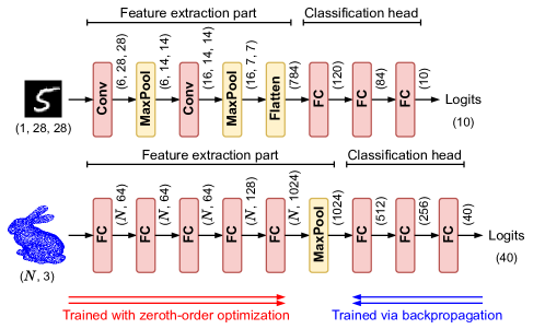
Figure 1: Overview of ElasticZO (top: LeNet-5, bottom: PointNet). ElasticZO trains the first $C$ layers with ZO optimization and the last $L-C$ layers with BP. Red and yellow rectangles denote layers with and without trainable parameters.

Algorithm 1 Training with ElasticZO

1:Network ${\bf\it\theta}$, partition point $C$, steps $T$, batch size $B$, perturbation scale $\varepsilon$, learning rate $\eta$

2:for $t=0,\ldots,T$ do

3: Sample a minibatch $\mathcal{B}$ (data $\mathcal{X}$ and label $\mathcal{Y}$) from a dataset $\mathcal{D}$

4: Sample a random seed $s$

5: PerturbParameters(${\bf\it\theta}$, $C$, $s$, $+1$, $\varepsilon$)

6: Run forward pass and compute a loss: $\ell_{+}=\mathcal{L}({\bf\it\theta};\mathcal{B})$

7: PerturbParameters(${\bf\it\theta}$, $C$, $s$, $-2$, $\varepsilon$)

8: Run forward pass and compute a loss: $\ell_{-}=\mathcal{L}({\bf\it\theta};\mathcal{B})$

9: Compute a zeroth-order gradient: $g\leftarrow\left(\ell_{+}-\ell_{-}\right)/2\varepsilon$

10: PerturbParameters(${\bf\it\theta}$, $C$, $s$, $+1$, $\varepsilon$)

11: ZOUpdateParameters(${\bf\it\theta}$, $C$, $s$, $\eta$, $g$)

12: BPUpdateParameters(${\bf\it\theta}$, $C$, $({\bf\it a}_{C},\ldots,{\bf\it a}_{L})$, $\mathcal{Y}$)

13:function PerturbParameters(${\bf\it\theta}$, $C$, $s$, $k$, $\varepsilon$)

14: Initialize a pseudorandom number generator with a seed $s$

15: for $l=1,\ldots,C$ do

16:  Generate a random vector: ${\bf\it z}_{l}\sim\mathcal{N}(\mathbf{0},\mathbf{I})$

17:  Perturb parameters in-place: ${\bf\it\theta}_{l}\leftarrow{\bf\it\theta}_{l}+k\varepsilon{\bf\it z}_{l}$  

18:function ZOUpdateParameters(${\bf\it\theta}$, $C$, $s$, $\eta$, $g$)

19: Initialize a pseudorandom number generator with a seed $s$

20: for $l=1,\ldots,C$ do

21:  Generate a random vector: ${\bf\it z}_{l}\sim\mathcal{N}(\mathbf{0},\mathbf{I})$

22:  Update parameters in-place: ${\bf\it\theta}_{l}\leftarrow{\bf\it\theta}_{l}-\eta g{\bf\it z}_{l}$  

23:function BPUpdateParameters(${\bf\it\theta}$, $C$, ${\bf\it a}$, $\mathcal{Y}$)

24: Compute a gradient of last layer output ${\bf\it e}_{L}$ using ${\bf\it a}_{L}$ and $\mathcal{Y}$

25: for $l=L,L-1,\ldots,C+1$ do

26:  Compute a gradient of parameters ${\bf\it g}_{l}$ using ${\bf\it a}_{l-1}$ and ${\bf\it e}_{l}$

27:  Compute a gradient of previous layer output ${\bf\it e}_{l-1}$ using ${\bf\it\theta}_{l}$ and ${\bf\it e}_{l}$  

28: Update parameters ${\bf\it\theta}_{C+1},\ldots,{\bf\it\theta}_{L}$ via a FO optimizer (e.g., SGD)

Let $f({\bf\it\theta})$ denote an $L$-layer DNN with layer parameters ${\bf\it\theta}=\left\{{\bf\it\theta}_{1},\ldots,{\bf\it\theta}_{L}\right\}$. As illustrated in Fig. 1, ElasticZO splits the given network into two parts, $\left\{{\bf\it\theta}_{1},\ldots,{\bf\it\theta}_{C}\right\}$ and $\left\{{\bf\it\theta}_{C+1},\ldots,{\bf\it\theta}_{L}\right\}$, and trains them via ZO and BP, respectively. ElasticZO can be viewed as an intermediate method between ZO and BP, and ElasticZO with $C=0$ and $C=L$ is equivalent to pure BP- and ZO-based training, respectively. We refer to these cases as Full BP and Full ZO. While inference engines are optimized for common operations needed during forward passes, such as matrix multiplication and convolution, they could still be used for backward passes as well, considering that backward passes involve similar types of operations (e.g., fully-connected (FC) layers perform matrix multiplications in both forward and backward passes).

As shown in Alg. 1, ElasticZO perturbs network parameters using in-place operations (lines 5, 7) and runs forward passes twice to compute losses $\ell_{+},\ell_{-}$ (lines 6, 8). These losses are used to obtain a gradient estimate $g$ (line 9). ElasticZO then updates parameters of the first $C$ layers using the estimated gradient $g$ via ZO (line 11) and those of the last $L-C$ layers via BP (line 12). For BP, ElasticZO keeps layer activations of the last $L-C+1$ layers $({\bf\it a}_{C},\ldots,{\bf\it a}_{L})$ obtained during the computation of $\ell_{+}$ and $\ell_{-}$. It is also possible to run another forward pass with the original unperturbed parameters to obtain layer activations, while this approach would require three forward passes per minibatch. Note that ZO parameter perturbation and update (lines 10–11) are merged into one step for efficiency, i.e., parameters are updated as ${\bf\it\theta}_{l}\leftarrow{\bf\it\theta}_{l}+(\varepsilon-\eta g){\bf\it z}_{l}\ (l\leq C)$.

4.1 Memory-Efficiency of ElasticZO

The memory consumption of ElasticZO depends on the partition point $C$ and lies in the middle between Full ZO and Full BP. Full BP requires to keep parameters, layer activations, and their gradients on the memory, and therefore the total memory cost is written as:

$$M_{\text{Full-BP}}=\sum_{l\in\mathcal{T}}\left(\left|{\bf\it\theta}_{l}\right|+\left|{\bf\it g}_{l}\right|\right)+\sum_{l=1}^{L}\left(\left|{\bf\it a}_{l}\right|+\left|{\bf\it e}_{l}\right|\right),$$ (2)

where $\mathcal{T}\subseteq\left\{1,\ldots,L\right\}$ denotes a set of layers with learnable parameters (i.e., FC and convolution layers, red rectangles in Fig. 1). Note that the memory cost can be reduced by considering the lifetime of each variable (e.g., an error ${\bf\it e}_{l}$ can be discarded after ${\bf\it g}_{l}$ and ${\bf\it e}_{l-1}$ are computed). For ease of analysis, we assume that such optimization is not applied here and thus buffers for all necessary variables remain allocated on memory during the whole training process. In Full ZO ($C=L$), no extra buffer is needed for gradients and errors as parameters can be updated in-place, and only parameters and layer activations are stored on memory as a result. The total memory consumption becomes:

$$M_{\text{Full-ZO}}=\sum_{l\in\mathcal{T}}\left|{\bf\it\theta}_{l}\right|+\sum_{l=1}^{L}\left|{\bf\it a}_{l}\right|.$$ (3)

While layer activations ${\bf\it a}$ can be immediately released after being used by subsequent layers during forward passes, such dynamic memory management is not considered as above to simplify the analysis. Eqs. 2–3 indicate that Full BP takes twice the memory for inference due to gradients ${\bf\it g},{\bf\it e}$, while Full ZO only consumes the same amount of memory as inference and thus halves the memory footprint than Full BP. ElasticZO stores parameters and activations, as well as gradients of the last layers for BP. The total memory consumption is given by:

$$M_{\text{{ElasticZO}}}=\sum_{l\in\mathcal{T}}\left|{\bf\it\theta}_{l}\right|+\sum_{l=1}^{L}\left|{\bf\it a}_{l}\right|+\sum_{\begin{subarray}{c}l\in\mathcal{T}\\ l\geq C+1\end{subarray}}\left|{\bf\it g}_{l}\right|+\sum_{l=C+1}^{L}\left|{\bf\it e}_{l}\right|.$$ (4)

This leads to an inequality $M_{\text{Full-ZO}}\leq M_{\text{{ElasticZO}}}\leq M_{\text{Full-BP}}$, where the equality holds if $C=0,L$. The partition point $C$ controls the trade-off between memory usage and accuracy. Reducing $C$ and training more parts of the network with BP will yield an improved accuracy at the cost of higher memory usage ($M_{\text{{ElasticZO}}}$ approaches to $M_{\text{Full-BP}}$). Evaluation results (Sec. 5) empirically show that ElasticZO with $C=L-1,L-2$ (i.e., training the last one or two layers with BP and the others with ZO) achieves an accuracy similar to Full BP, while maintaining memory consumption close to that of Full ZO.

The memory consumption depends on the choice of optimizer as well. If an optimizer does not have any states (e.g., SGD), the memory consumption can be obtained from Eqs. 2–4. More advanced optimizers consume additional memory to save optimizer states. For instance, Adam [5] needs to keep track of first- and second-order gradient moments that take up twice the memory of trainable parameters. In such case, the memory consumption of Full BP is computed as:

$$M_{\text{Full-BP-Adam}}=M_{\text{Full-BP}}+2\sum_{l\in\mathcal{T}}\left|{\bf\it g}_{l}\right|.$$ (5)

4.2 INT8 Training with ElasticZO-INT8

To further improve computational and memory-efficiency, we propose ElasticZO-INT8 as a variant of ElasticZO that only involves 8-bit integer arithmetic. ElasticZO-INT8 integrates the recently-proposed framework for 8-bit integer training, NITI [42], with ZO gradient estimation. In NITI, variables (e.g., parameters and activations) are represented in the form of ${\bf\it v}^{\text{int8}}\cdot 2^{s}$ and hence stored as a pair of 8-bit signed integers and a scaling exponent $({\bf\it v}^{\text{int8}},s)$. The 8-bit integers are scaled by $2^{s}$, and hence the exponent is crucial for dynamically adjusting the representable value range during training.

Algorithm 2 Training with ElasticZO-INT8

1:Network ${\bf\it\theta}^{\text{int8}}$, partition point $C$, steps $T$, batch size $B$, perturbation scale $r_{\max}$, sparsity $p_{\text{zero}}$, gradient bitwidth $b_{\text{ZO}}$ (for ZO), $b_{\text{BP}}$ (for BP)

2:for $t=0,\ldots,T$ do

3: Sample a batch $\mathcal{B}$ (data $\mathcal{X}$ and label $\mathcal{Y}$) from a dataset $\mathcal{D}$

4: Sample a random seed $s$

5: PerturbParametersInt8(${\bf\it\theta}^{\text{int8}}$, $C$, $s$, $+1$, $r_{\max}$, $p_{\text{zero}}$)

6: Run forward pass and compute 8-bit integer logits: ${\bf\it a}_{L}^{\text{int8},+}=f({\bf\it\theta}^{\text{int8}})$

7: PerturbParametersInt8(${\bf\it\theta}^{\text{int8}}$, $C$, $s$, $-2$, $r_{\max}$, $p_{\text{zero}}$)

8: Run forward pass and compute 8-bit integer logits: ${\bf\it a}_{L}^{\text{int8},-}=f({\bf\it\theta}^{\text{int8}})$

9: Compute a zeroth-order gradient: $g\leftarrow\operatorname{sgn}(\ell_{+}-\ell_{-})=\operatorname{sgn}(\mathcal{L}({\bf\it a}_{L}^{\text{int8},+},\mathcal{B})-\mathcal{L}({\bf\it a}_{L}^{\text{int8},-},\mathcal{B}))$

10: PerturbParametersInt8(${\bf\it\theta}^{\text{int8}}$, $C$, $s$, $+1$, $r_{\max}$, $p_{\text{zero}}$)

11: ZOUpdateParametersInt8(${\bf\it\theta}^{\text{int8}}$, $C$, $s$, $g$, $b_{\text{ZO}}$)

12: BPUpdateParametersInt8(${\bf\it\theta}^{\text{int8}}$, $C$, $({\bf\it a}_{C}^{\text{int8}},\ldots,{\bf\it a}_{L}^{\text{int8}})$, $\mathcal{Y}$)

13:function PerturbParametersInt8(${\bf\it\theta}$, $C$, $s$, $k$, $r_{\max}$, $p_{\text{zero}}$)

14: Initialize a pseudorandom number generator with a seed $s$

15: for $l=1,\ldots,C$ do

16:  Generate a random mask and vector: ${\bf\it m}\sim\text{Bernoulli}(1-p_{\text{zero}}),\ {\bf\it u}^{\text{int8}}\sim\mathcal{U}(-r_{\max},r_{\max})$

17:  Create a sparse random vector: ${\bf\it z}_{l}^{\text{int8}}\leftarrow{\bf\it m}\odot{\bf\it u}^{\text{int8}}$

18:  Perturb parameters in-place: ${\bf\it\theta}_{l}^{\text{int8}}\leftarrow\text{Clamp}({\bf\it\theta}_{l}^{\text{int8}}+k{\bf\it z}_{l}^{\text{int8}},-127,127)$  

19:function ZOUpdateParametersInt8(${\bf\it\theta}$, $C$, $s$, $g$, $b_{\text{ZO}}$)

20: Initialize a pseudorandom number generator with a seed $s$

21: for $l=1,\ldots,C$ do

22:  Generate a random mask and vector: ${\bf\it m}\sim\text{Bernoulli}(1-p_{\text{zero}}),\ {\bf\it u}^{\text{int8}}\sim\mathcal{U}(-r_{\max},r_{\max})$

23:  Create a sparse random vector: ${\bf\it z}_{l}^{\text{int8}}\leftarrow{\bf\it m}\odot{\bf\it u}^{\text{int8}}$

24:  Compute an update: ${\bf\it g}^{\text{int8}}\leftarrow\text{PseudoStochasticRound}(g{\bf\it z}_{l}^{\text{int8}},b_{\text{ZO}})$

25:  Update parameters in-place: ${\bf\it\theta}_{l}^{\text{int8}}\leftarrow\text{Clamp}({\bf\it\theta}_{l}^{\text{int8}}-{\bf\it g}^{\text{int8}},-127,127)$  

Unlike ElasticZO, ElasticZO-INT8 performs each step in Alg. 1 entirely with integer arithmetic. The resulting algorithm is outlined in Alg. 2. Let $f({\bf\it\theta}^{\text{int8}})$ denote an 8-bit quantized network with ${\bf\it\theta}^{\text{int8}}=\left\{({\bf\it\theta}_{l}^{\text{int8}},s_{\theta,l})\right\}_{l=1}^{L}$ being layer parameters (8-bit integers) and their associated exponents (scalars). Similar to ElasticZO, ElasticZO-INT8 first runs two forward passes (lines 6, 8) using perturbed parameters (lines 5, 7) and keeps outputs of the last layer ${\bf\it a}_{L}^{\text{int8},+},{\bf\it a}_{L}^{\text{int8},-}$. It computes a zeroth-order gradient $g$ using these logits (line 9) and restores the unperturbed parameters (line 10). The parameters of the first $C$ layers are updated with ZO (line 11) and those of the last $L-C$ layers with BP (line 12), respectively.

Parameter perturbation (lines 13–18): In Full ZO and ElasticZO, parameters are perturbed with a standard Gaussian random vector ${\bf\it z}\sim\mathcal{N}(\mathbf{0},\mathbf{I})$. ElasticZO-INT8 instead samples a random INT8 vector ${\bf\it u}^{\text{int8}}$ from a uniform distribution $\mathcal{U}(-r_{\max},r_{\max})$, since NITI adopts a uniform initialization of parameters to achieve better accuracy with a limited value range [42]. In addition, the vector ${\bf\it u}^{\text{int8}}$ is made sparse by randomly setting $p_{\text{zero}}$% of its entries to zeros using a binary mask ${\bf\it m}\sim\text{Bernoulli}(1-p_{\text{zero}})$. This can be viewed as a random dropout in standard BP training. The resulting sparse perturbation ${\bf\it z}^{\text{int8}}={\bf\it m}\odot{\bf\it u}^{\text{int8}}$ is applied to parameters ${\bf\it\theta}_{l}^{\text{int8}}$ and they are clipped to the INT8 range.

Parameter update via ZO (lines 19–25): Given a learning rate $\eta$ and zeroth-order gradient $g$, ElasticZO computes an update to the parameter as $-\eta g{\bf\it z}$. Following NITI, ElasticZO-INT8 first computes a product $g{\bf\it z}^{\text{int8}}$ and rounds it to $b_{\text{ZO}}$-bit using a pseudo-stochastic rounding scheme (refer to [42] for details of rounding) to obtain an update ${\bf\it g}^{\text{int8}}$. The bitwidth $b_{\text{ZO}}$ determines a magnitude of an update and hence works as a learning rate. With a scaling exponent $s_{\theta}$ for parameters ${\bf\it\theta}^{\text{int8}}$, the update is actually written as ${\bf\it g}^{\text{int8}}\cdot 2^{s_{\theta}}$ ($s_{\theta}$ is fixed throughout the training process as in NITI). Note that parameters can be updated in-place and thus no extra memory is required for intermediate variables (${\bf\it m},{\bf\it u}^{\text{int8}},{\bf\it z}_{l}^{\text{int8}},{\bf\it g}^{\text{int8}}$).

Forward and backward passes (lines 6, 8, 12): Forward and backward passes follow the NITI framework. In the forward pass, an input is first converted to the form of ${\bf\it a}_{0}\cdot 2^{s_{a,0}}$ before fed to the network. A FC or convolution layer performs matrix product or convolution between parameters ${\bf\it\theta}_{l}^{\text{int8}}$ and an input ${\bf\it a}_{l-1}^{\text{int8}}$ in integer arithmetic and stores the result ${\bf\it a}_{l}^{\text{int32}}$ in 32-bit integer format. Besides, a scaling exponent of an output is obtained by adding exponents of the parameters and input, i.e., $s_{a,l}=s_{\theta,l}+s_{a,l-1}$. The output is rounded to 8-bit ${\bf\it a}_{l}^{\text{int8}}$ and the exponent is updated accordingly. In this rounding process, the minimum bitwidth required to represent values in ${\bf\it a}_{l}^{\text{int32}}$ is determined as $b=\lfloor\log_{2}(\max(\absolutevalue{{\bf\it a}_{l}^{\text{int32}}}))\rfloor+1$, where $\max(\absolutevalue{{\bf\it a}_{l}^{\text{int32}}})$ denotes the maximum absolute value in ${\bf\it a}_{l}^{\text{int32}}$. In case of $b>7$, values in ${\bf\it a}_{l}^{\text{int32}}$ is right-shifted by $b-7$-bit and $b-7$ is added to the exponent $s_{\theta,l}$. Refer to [42] for a rounding procedure and backward pass. Similar to ZO, an update to the parameter is rounded to $b_{\text{BP}}$-bit.

4.3 Zeroth-order Gradient Estimation with Integer Arithmetic

In ZO training, the zeroth-order gradient $g$ is derived from the difference between two cross-entropy losses $\ell_{+},\ell_{-}$. NITI only proposes an integer arithmetic-only method to approximate a gradient of the integer cross-entropy loss $\mathcal{L}({\bf\it a}_{L}^{\text{int8}})$ with respect to its logits ${\bf\it a}_{L}^{\text{int8}}$, and circumvents an evaluation of the loss value itself. $\mathcal{L}$ involves a log-sum-exp function and seems challenging to compute it using integer arithmetic only. In addition, since an update ${\bf\it g}^{\text{int8}}$ is obtained by rounding a product $g{\bf\it z}$ to $b_{\text{ZO}}$-bit, the magnitude of zeroth-order gradient $g$ does not affect ${\bf\it g}^{\text{int8}}$ (e.g., ${\bf\it z}$, $2{\bf\it z}$, and $4{\bf\it z}$ are likely to produce the same update vector after rounding). Considering these, we propose to only evaluate a sign of difference between two losses $\operatorname{sgn}(\ell_{+}-\ell_{-})$ and use it as a ternary gradient $g\in\left\{-1,0,+1\right\}$. Besides, losses $\ell_{+},\ell_{-}$ can be computed using floating-point as a simple workaround.

Let $({\bf\it\alpha}^{\text{int8}},s_{\alpha})$ and $({\bf\it\beta}^{\text{int8}},s_{\beta})$ denote 8-bit integer logits (i.e., outputs of the network $f({\bf\it\theta}^{\text{int8}})$) along with their scaling factors. The cross-entropy loss is written as:

$$\mathcal{L}({\bf\it\alpha}^{\text{int8}};\mathcal{Y})=-\ln\frac{\exp(\alpha_{i}^{\text{int8}}\cdot 2^{s_{\alpha}})}{\sum_{j}\exp(\alpha_{j}^{\text{int8}}\cdot 2^{s_{\alpha}})},\quad\mathcal{L}({\bf\it\beta}^{\text{int8}};\mathcal{Y})=-\ln\frac{\exp(\beta_{i}^{\text{int8}}\cdot 2^{s_{\beta}})}{\sum_{j}\exp(\beta_{j}^{\text{int8}}\cdot 2^{s_{\beta}})},$$ (6)

where $i$ is a label of the input. We modify Eq. 6 as:

$$\mathcal{L}({\bf\it\alpha}^{\text{int8}};\mathcal{Y})=\ln\sum_{j}\exp(\left(\alpha_{j}^{\text{int8}}-\alpha_{i}^{\text{int8}}\right)\cdot 2^{s_{\alpha}}),\quad\mathcal{L}({\bf\it\beta}^{\text{int8}};\mathcal{Y})=\ln\sum_{j}\exp(\left(\beta_{j}^{\text{int8}}-\beta_{i}^{\text{int8}}\right)\cdot 2^{s_{\beta}}).$$ (7)

For simplicity, we define a new scaling factor as $s=\min(s_{\alpha},s_{\beta})$ and rewrite terms in Eq. 7 using rescaled logits $\bar{\alpha}_{j}^{\text{int8}}=\alpha_{j}^{\text{int8}}\cdot 2^{s_{\alpha}-s}$, $\bar{\beta}_{j}^{\text{int8}}=\beta_{j}^{\text{int8}}\cdot 2^{s_{\beta}-s}$:

$$\exp(\left(\alpha_{j}^{\text{int8}}-\alpha_{i}^{\text{int8}}\right)\cdot 2^{s_{\alpha}})=\exp(\left(\bar{\alpha}_{j}^{\text{int8}}-\bar{\alpha}_{i}^{\text{int8}}\right)\cdot 2^{s}),\ \exp(\left(\beta_{j}^{\text{int8}}-\beta_{i}^{\text{int8}}\right)\cdot 2^{s_{\beta}})=\exp(\left(\bar{\beta}_{j}^{\text{int8}}-\bar{\beta}_{i}^{\text{int8}}\right)\cdot 2^{s}).$$ (8)

To evaluate the above with integer operations, we replace $\exp(x)$ with a power of two $2^{(\log_{2}e)\cdot x}$ and approximate $\log_{2}e$ by integer multiplication and bit-shift $\log_{2}e\approx 47274\cdot 2^{-15}$, as discussed in [42]. This yields the following:

$$\exp(\left(\bar{\alpha}_{j}^{\text{int8}}-\bar{\alpha}_{i}^{\text{int8}}\right)\cdot 2^{s})=2^{47274\left(\bar{\alpha}_{j}^{\text{int8}}-\bar{\alpha}_{i}^{\text{int8}}\right)\cdot 2^{s-15}}=2^{\hat{\alpha}_{j}},\ \exp(\left(\bar{\beta}_{j}^{\text{int8}}-\bar{\beta}_{i}^{\text{int8}}\right)\cdot 2^{s})=2^{47274\left(\bar{\beta}_{j}^{\text{int8}}-\bar{\beta}_{i}^{\text{int8}}\right)\cdot 2^{s-15}}=2^{\hat{\beta}_{j}}.$$ (9)

The exponent $\hat{\alpha}_{j},\hat{\beta}_{j}$ may still be large and cause an integer overflow. For numerical stability, we offset each exponent by $p=p_{\max}-10$ ($p_{\max}=\max(\max_{j}(\hat{\alpha}_{j}),\max_{j}(\hat{\beta}_{j}))$) and define a new exponent as $\tilde{\alpha}_{j}=\max(\hat{\alpha}_{j}-p,0),\tilde{\beta}_{j}=\max(\hat{\beta}_{j}-p,0)$, such that $2^{\tilde{\alpha}_{j}},2^{\tilde{\beta}_{j}}\leq 2^{10}$ holds for any $j$ [42]. The term $2^{x}$ with an exponent $x<p$ can be safely ignored as it is at least $2^{10}$ times smaller than the maximum term $2^{p_{\max}}=2^{p+10}$ and has little effect on the final result. With these notations, the loss difference can be written as:

$$\mathcal{L}({\bf\it\alpha}^{\text{int8}};\mathcal{Y})-\mathcal{L}({\bf\it\beta}^{\text{int8}};\mathcal{Y})=\ln\frac{\sum_{j}\exp(\left(\alpha_{j}^{\text{int8}}-\alpha_{i}^{\text{int8}}\right)\cdot 2^{s_{\alpha}})}{\sum_{j}\exp(\left(\beta_{j}^{\text{int8}}-\beta_{i}^{\text{int8}}\right)\cdot 2^{s_{\beta}})}=\ln\frac{\sum_{j}2^{\tilde{\alpha}_{j}}}{\sum_{j}2^{\tilde{\beta}_{j}}}.$$ (10)

Eq. 10 involves evaluating a ratio of sums of terms (approximated as powers of two) and taking its natural logarithm. Since it seems challenging to obtain an accurate result in a form of $x\cdot 2^{s}$ using integer arithmetic only, we consider a sign of loss difference and use it as a gradient $g$ (Alg. 2, line 9). The sign can be easily obtained by comparing two terms $\sum_{j}2^{\tilde{\alpha}_{j}},\sum_{j}2^{\tilde{\beta}_{j}}$ without logarithm operations. Similarly, ZO-signSGD [25] uses a sign information of the zeroth-order gradient estimate to mitigate the effect of gradient noise and improve robustness of ZO training.

If a batch size $B$ is greater than one, the loss difference has the following form:

$$\mathcal{L}({\bf\it\alpha}^{\text{int8}};\mathcal{Y})-\mathcal{L}({\bf\it\beta}^{\text{int8}};\mathcal{Y})=\sum_{b}\ln\frac{\sum_{j}\exp(\left(\alpha_{b,j}^{\text{int8}}-\alpha_{b,t(b)}^{\text{int8}}\right)\cdot 2^{s_{\alpha,b}})}{\sum_{j}\exp(\left(\beta_{b,j}^{\text{int8}}-\beta_{b,t(b)}^{\text{int8}}\right)\cdot 2^{s_{\beta,b}})}=\sum_{b}\ln\frac{\sum_{j}2^{\tilde{\alpha}_{b,j}}}{\sum_{j}2^{\tilde{\beta}_{b,j}}},$$ (11)

where $b$ denotes a sample index in a minibatch and $t(b)$ a label for the $b$-th sample. In this case, we use Eq. 12 to evaluate a sign:

$$\mathcal{L}({\bf\it\alpha}^{\text{int8}};\mathcal{Y})-\mathcal{L}({\bf\it\beta}^{\text{int8}};\mathcal{Y})=\ln 2\cdot\left(\sum_{b}\lfloor\log_{2}\sum_{j}2^{\tilde{\alpha}_{b,j}}\rfloor-\sum_{b}\lfloor\log_{2}\sum_{j}2^{\tilde{\beta}_{b,j}}\rfloor\right).$$ (12)

Note that $\lfloor\log_{2}n\rfloor$ is easily obtained by counting the number of leading zero bits in $n$. While the use of floor operation $\lfloor\cdot\rfloor$ may lead to incorrect results, we empirically find that correct signs can be obtained at a high probability ($\sim$95%).

4.4 Memory-Efficiency of ElasticZO-INT8

ElasticZO-INT8 with $C=0$ (Full BP) is equivalent to the baseline NITI (ElasticZO-INT8 with $C=L$ (Full ZO) is a ZO-based 8-bit training algorithm). While 8-bit integers are used, a FC or convolution layer requires extra buffers to store intermediate multiply-accumulation results (32-bit integers) when computing an activation ${\bf\it a}_{l}$, gradient ${\bf\it g}_{l}$, and error ${\bf\it e}_{l-1}$. In NITI, the maximum absolute value of an input tensor ${\bf\it x}^{\text{int32}}$ should be obtained first before rounding its elements to 8-bit and adjusting a scaling factor, necessitating a buffer to store the whole input tensor. As a result, the total memory consumption is formulated as:

$$M_{\text{Full-BP-Int8}} =\sum_{l\in\mathcal{T}}\left(\left|{\bf\it\theta}_{l}^{\text{int8}}\right|+\left|{\bf\it g}_{l}^{\text{int8}}\right|\right)+\sum_{l=1}^{L}\left(\left|{\bf\it a}_{l}^{\text{int8}}\right|+\left|{\bf\it e}_{l}^{\text{int8}}\right|\right)+\sum_{l\in\mathcal{T}}\left(\left|{\bf\it a}_{l}^{\text{int32}}\right|+\left|{\bf\it g}_{l}^{\text{int32}}\right|\right)+\sum_{\begin{subarray}{c}l\in\mathcal{T}\\ l>1\end{subarray}}\left|{\bf\it e}_{l-1}^{\text{int32}}\right|$$

$$=\frac{1}{4}M_{\text{Full-BP}}+\sum_{l\in\mathcal{T}}\left(\left|{\bf\it a}_{l}^{\text{int32}}\right|+\left|{\bf\it g}_{l}^{\text{int32}}\right|\right)+\sum_{\begin{subarray}{c}l\in\mathcal{T}\\ l>1\end{subarray}}\left|{\bf\it e}_{l-1}^{\text{int32}}\right|.$$ (13)

In case of $C=L$ (i.e., all layers are trained via ZO), gradients and errors are not needed to be kept on memory as parameters are updated in-place, leading to the reduced memory usage:

$$M_{\text{Full-ZO-Int8}}=\sum_{l\in\mathcal{T}}\left|{\bf\it\theta}_{l}^{\text{int8}}\right|+\sum_{l=1}^{L}\left|{\bf\it a}_{l}^{\text{int8}}\right|+\sum_{l\in\mathcal{T}}\left|{\bf\it a}_{l}^{\text{int32}}\right|=\frac{1}{4}M_{\text{Full-ZO}}+\sum_{l\in\mathcal{T}}\left|{\bf\it a}_{l}^{\text{int32}}\right|.$$ (14)

This indicates the memory usage is reduced by more than half and equals to the inference. ElasticZO-INT8 stores parameters and activations for all layers, as well as gradients and errors for the last $L-C+1$ layers, which gives the total memory cost:

$$M_{\text{{ElasticZO-INT8}}} =\sum_{l\in\mathcal{T}}\left|{\bf\it\theta}_{l}^{\text{int8}}\right|+\sum_{l=1}^{L}\left|{\bf\it a}_{l}^{\text{int8}}\right|+\sum_{\begin{subarray}{c}l\in\mathcal{T}\\ l\geq C+1\end{subarray}}\left|{\bf\it g}_{l}^{\text{int8}}\right|+\sum_{l=C+1}^{L}\left|{\bf\it e}_{l}^{\text{int8}}\right|$$

$$\phantom{=}+\sum_{l\in\mathcal{T}}\left|{\bf\it a}_{l}^{\text{int32}}\right|+\sum_{\begin{subarray}{c}l\in\mathcal{T}\\ l\geq C+1\end{subarray}}\left|{\bf\it g}_{l}^{\text{int32}}\right|+\sum_{\begin{subarray}{c}l\in\mathcal{T}\\ l>C+1\end{subarray}}\left|{\bf\it e}_{l-1}^{\text{int32}}\right|$$

$$=\frac{1}{4}M_{\text{{ElasticZO}}}+\sum_{l\in\mathcal{T}}\left|{\bf\it a}_{l}^{\text{int32}}\right|+\sum_{\begin{subarray}{c}l\in\mathcal{T}\\ l\geq C+1\end{subarray}}\left|{\bf\it g}_{l}^{\text{int32}}\right|+\sum_{\begin{subarray}{c}l\in\mathcal{T}\\ l>C+1\end{subarray}}\left|{\bf\it e}_{l-1}^{\text{int32}}\right|.$$ (15)

Similar to Sec. 4.1, this gives an inequality $M_{\text{Full-ZO-Int8}}\leq M_{\text{{ElasticZO-INT8}}}\leq M_{\text{Full-BP-Int8}}$, and therefore the memory footprint of ElasticZO-INT8 is in the middle between that of Full BP and Full ZO. In addition, the memory usage of the INT8 version is not equal to a quarter of the FP32 case (Eqs. 2–4) due to additional buffers for intermediate results. Recall that the memory usage can be further reduced by taking into account the lifetime of variables and reusing the same buffer for variables with a non-overlapping lifetime (e.g., ${\bf\it e}_{l}^{\text{int8}}$ and ${\bf\it e}_{l-2}^{\text{int8}}$ in Eq. 13 and ${\bf\it a}_{l}^{\text{int32}}$ and ${\bf\it a}_{l+2}^{\text{int32}}$ in Eq. 14). Such memory optimization techniques are well-studied and orthogonal to our work. We plan to improve Eqs. 2–4 and Eqs. 13–15 in a future work.

5 Evaluation

In this section, we evaluate ElasticZO and ElasticZO-INT8 in terms of three aspects: accuracy, memory-efficiency, and execution time. We compare the performance of proposed methods with Full ZO and Full BP in both FP32 and INT8 cases.

5.1 Experimental Setup

ElasticZO, ElasticZO-INT8, as well as Full BP and Full ZO are implemented with PyTorch. The INT8 version is based on the publicly available code of NITI [42]. For accuracy evaluation, we use a workstation with an eight-core 3.8GHz Intel Core i7-10700K CPU, a 32GB of DRAM, and an Nvidia GeForce RTX 3090 GPU running Ubuntu 20.04. We conduct experiments on PyTorch 2.5.0 and CUDA 12.1.

In addition, ElasticZO and ElasticZO-INT8 are implemented in C++ and cross-compiled with -O3 optimization flag using ARM GCC toolchain 12.2. We employ vectorization with ARM NEON intrinsics and multithreading with OpenMP library to fully utilize CPU cores. The training code is executed on a Raspberry Pi Zero 2 board with a four-core 1GHz ARM Cortex-A72 CPU and a 512MB of DRAM running Raspberry Pi OS (based on Debian 12). Note that the CPU frequency is fixed at 1GHz to accurately measure the execution time.

As for datasets, we use MNIST [43], Fashion-MNIST [44], and ModelNet40 [45, 46] in the evaluation. The former two are widely-known image classification datasets, each consisting of $50\,000$ 28$\times$28 grayscale images for training and $10\,000$ images for testing. On the other hand, ModelNet40 [45, 46] is a 3D point cloud dataset containing $12\,311$ samples from 40 object categories ($9843$ for training and $2468$ for testing). Each sample consists of $2048$ points that are randomly sampled from a synthetic 3D model and normalized to have a zero centroid and a unit radius. When evaluating a fine-tuning performance, we additionally use Rotated MNIST and Rotated Fashion-MNIST [47, 48]. We randomly choose $1024$ images from train and test splits and rotate them by either $30^{\circ}$ or $45^{\circ}$.

5.1.1 Details of DNN Models and Training

We train LeNet-5 [43] and PointNet [46] on MNIST and ModelNet40 datasets, respectively. LeNet-5 (Fig. 1, top) consists of a stack of two convolution layers followed by three FC layers. In ElasticZO and ElasticZO-INT8, we consider setting the partition point to $C=L-1,L-2$. That is, we consider training (i) two convolution layers and the first FC layer, or (ii) two convolution layers and the first two FC layers via ZO, and the remaining one or two FC layers via BP. As a result, 89.8% and 99.2% of parameters ($96\,772$ and $106\,936$ out of $107\,786$) are trained via ZO. We refer to these configurations as ZO-Feat-Cls1 and ZO-Feat-Cls2. PointNet (Fig. 1, bottom) is a DNN tailored for point cloud tasks and directly takes 3D point coordinates as input. The feature extraction part consists of five FC layers and one max-pooling layer, while the classification head is a stack of three FC layers. Similar to LeNet-5, we train convolution layers as well as the first (i) one or (ii) two FC layers via ZO, meaning that ZO handles 82.7% and 98.7% of the parameters ($675\,136$ and $806\,464$ out of $816\,744$), respectively. Note that 8-bit models do not have bias parameters as in NITI [42].

Throughout the evaluation, we use vanilla SGD optimizer without momentum or weight decay for updating parameters. The number of epochs is set to $E=100,200$ when training LeNet-5 and PointNet from scratch, respectively. We describe the training details below.

FP32 case: For each model and dataset, the initial learning rate $\eta$ is tuned in the range $[\text{1e-4},\text{5e-2}]$. It is decayed by a factor of 0.8 every 10 epochs. The batch size is set to $B=32$. In ZO training, we clip a ZO gradient $g$ within the range $[-g_{\text{clip}},g_{\text{clip}}]$ to stabilize training.

INT8 case: Following NITI [42], the gradient bitwidth $b_{\text{BP}}$ (for BP) is first set to 5 and then decreased to 4 and 3 at 20 and 50 epochs, respectively. The batch size is set to $B=256$. In ZO training, the perturbation scale $\varepsilon$ is tuned in the range $[1,3,7,15,31,63]$ for each experiment, while the gradient bitwidth $b_{\text{ZO}}$ is fixed to 1. The sparsity $p_{\text{zero}}$ is initialized with 0.33 and increased to 0.5 and 0.9 at 20 and 50 epochs, respectively.

5.2 Accuracy on Classification Datasets

Table 1 (columns 1–6) shows the classification accuracy of LeNet-5 on MNIST and Fashion-MNIST. INT8 and INT8* denote that ZO gradients $g$ are obtained using floating-point and integer arithmetic, respectively (Sec. 4.3). As a result, INT8* performs an integer arithmetic-only training. We evaluate the accuracy of FP32 and INT8 methods using the PyTorch implementation and that of INT8* counterpart using C++ version.

In the FP32 case (columns 1, 4), Full ZO gives 9.3–14.3% lower accuracy than Full BP, which is attributed to a large noise in ZO gradients $g$. On the other hand, by training the last one or two FC layers (i.e., 0.8% and 10.2% of LeNet-5 parameters) via BP, ZO-Feat-Cls2 and ZO-Feat-Cls1 improve the accuracy by 5.1–5.2% and 7.7–9.5% with a negligible execution time and memory overhead (Figs. 4 and 7). As a result, ZO-Feat-Cls2 and ZO-Feat-Cls1 shrink the accuracy gap to 4.3–9.1% and 1.6–4.8%, respectively. In the INT8 case (columns 2–3, 5–6), Full ZO shows 9.0–16.4% lower accuracy than Full BP. ZO-Feat-Cls2 and ZO-Feat-Cls1 produce 7.6–10.7% and 4.6–6.4% higher accuracy than Full ZO, reducing the accuracy gap to 4.4–10.1% and 1.4–5.7%, respectively. These results indicate that ElasticZO and ElasticZO-INT8 address the low accuracy of Full ZO with a little help from BP.

As seen in columns 1–2 and 4–5, ElasticZO-INT8 provides nearly the same or comparable accuracy to that of ElasticZO while improving memory-efficiency (Fig. 5). The accuracy difference is at most 0.5% and 2.0% in MNIST and Fashion-MNIST, respectively. The proposed integer-only gradient estimation (INT8*, Sec. 4.3) leads to 0.4–1.5% and 2.4–3.1% accuracy drop in MNIST and Fashion-MNIST, respectively, due to incorrect estimation results (around 5% of the time). Despite that, it still preserves a comparable level of accuracy as the floating-point counterpart as seen in columns 2–3 and 5–6.

The accuracy of PointNet on ModelNet40 is presented in Table 1 (column 7). Full ZO fails to achieve satisfactory accuracy when training PointNet (which has 7.6x more parameters than LeNet-5) from random initialization. Compared to that, ElasticZO largely outperforms Full ZO and also shows a comparable or even better accuracy to Full BP by training only the last few FC layers via BP.

ElasticZO-INT8 achieves better prediction accuracy by gradually increasing a sparsity of parameter updates $p_{\text{zero}}$ (Alg. 2, line 11) during training. For example, when $p_{\text{zero}}$ is fixed to the initial value (0.33) throughout the entire training process, Full ZO yields 9.5% and 6.3% lower accuracy on MNIST and Fashion-MNIST (80.26%/89.78% vs. 67.72%/73.98%), respectively.

Table 1: Accuracy of LeNet-5 (MNIST and Fashion-MNIST) and PointNet (ModelNet40)

	MNIST			Fashion-MNIST			ModelNet40
	FP32	INT8	INT8*	FP32	INT8	INT8*	FP32
Full ZO	89.80	89.78	88.92	77.09	73.98	71.02	32.05
ZO-Feat-Cls2	94.85	94.34	93.92	82.28	80.33	77.93	70.38
ZO-Feat-Cls1	97.53	97.34	95.83	86.60	84.66	81.60	73.50
Full BP	99.10	98.77	–	91.37	90.40	–	71.60

Table 2 shows fine-tuning results on MNIST datasets. In the FP32 case, LeNet-5 is first pre-trained on MNIST and Fashion-MNIST for a single epoch using BP. We use an Adam optimizer with an initial learning rate of $\eta=\text{1e-3}$ and momentum parameters of $\beta_{1}=0.9,\beta_{2}=0.999$. LeNet-5 is then fine-tuned on rotated datasets for additional 50 epochs. In the INT8 case, LeNet-5 is pre-trained on the original datasets for 100 epochs using BP (i.e., NITI) with a gradually decreasing gradient bit-width $b_{\text{BP}}$ (Sec. 5.1.1). In the fine-tuning step, LeNet-5 is trained for 50 more epochs on rotated datasets.

Without fine-tuning, the model suffers from a significant accuracy loss in case of a larger rotation angle ($\theta=45^{\circ}$), which is due to the discrepancy between training and test data distributions. Note that we do not employ data augmentation (e.g., random rotation) during pre-training, i.e., baseline models are not trained with rotated images. For FP32 models with Rotated MNIST (columns 1–2), fine-tuning with ZO-Feat-Cls2/ZO-Feat-Cls1 leads to 15.6/18.8% ($\theta=30^{\circ}$) and 39.7/45.0% ($\theta=45^{\circ}$) accuracy improvements. Similarly, in case of Rotated Fashion-MNIST (columns 3–4), fine-tuning with ZO-Feat-Cls2/ZO-Feat-Cls1 improves the prediction accuracy by 37.6/36.3% and 51.2/53.5%, respectively. By training a small fraction (10.2%) of the network via BP, ZO-Feat-Cls2 and ZO-Feat-Cls1 successfully bridge the accuracy gap between Full ZO and Full BP. As shown in columns 5–8, while Full ZO is affected by 8-bit quantization especially with Rotated Fashion-MNIST, ElasticZO-INT8 achieves an accuracy close to that of the full-precision counterparts. These results indicate that both ElasticZO and ElasticZO-INT8 can be used for fine-tuning as well as training from scratch and effectively handle the data distribution shift.

Table 2: Accuracy of LeNet-5 w/ or w/o fine-tuning on Rotated MNIST and Rotated Fashion-MNIST

	FP32				INT8
	Rotated MNIST		Rotated F-MNIST		Rotated MNIST		Rotated F-MNIST
	$30^{\circ}$	$45^{\circ}$	$30^{\circ}$	$45^{\circ}$	$30^{\circ}$	$45^{\circ}$	$30^{\circ}$	$45^{\circ}$
w/o Fine-tuning	74.41	46.58	39.65	23.34	84.08	60.25	28.13	13.77
Full ZO	85.94	74.71	61.33	59.08	85.94	64.36	37.21	22.95
ZO-Feat-Cls2	90.04	86.23	77.25	74.51	93.07	87.99	69.43	68.95
ZO-Feat-Cls1	93.16	91.60	75.98	76.86	93.46	91.80	76.07	75.68
Full BP	94.82	93.85	80.37	79.49	96.68	95.21	80.08	80.86

Fig. 2 shows training and test loss curves of the full-precision LeNet-5 on MNIST (left) and Fashion-MNIST (right). While Full ZO suffers from a slow convergence speed and seems to require far more than 100 epochs, ElasticZO is able to speed up the training process and close the performance gap to Full BP. Besides, ZO-Feat-Cls1 shows less fluctuations in the loss value compared to Full ZO, indicating that training the last FC layers with BP can stabilize training. Fig. 3 plots loss curves of the INT8 LeNet-5 over 100 epochs. The proposed ElasticZO-INT8 successfully trains LeNet-5 and achieves a loss close to that of Full BP on both datasets. ElasticZO-INT8 has a significantly lower loss at early epochs compared to Full ZO and thus our hybrid approach is more effective in case of limited precision. Note that the loss drops sharply at around 20 and 50 epochs, which is possibly due to changes in the hyperparameter settings ($p_{\text{zero}}$, Sec. 5.1.1).

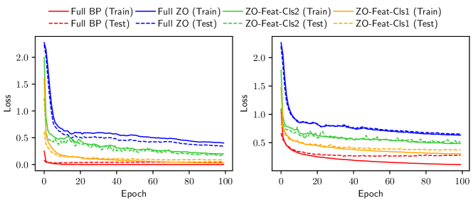
Figure 2: Training and test loss curves of LeNet-5 (FP32; left: MNIST, right: Fashion-MNIST).

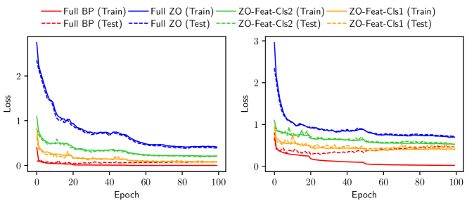
Figure 3: Training and test loss curves of LeNet-5 (INT8; left: MNIST, right: Fashion-MNIST).

5.3 Memory-Efficiency

Fig. 4 shows the memory usage breakdown of full-precision ElasticZO in comparison with Full BP and Full ZO computed using Eqs. 2–4. We consider LeNet-5 trained on MNIST with a batch size of $B=32,256$. As discussed in Sec. 4.1, Full BP has the largest memory footprint, because it needs to store gradients and errors ${\bf\it g},{\bf\it e}$ for all layers as well as parameters and activations ${\bf\it\theta},{\bf\it a}$ (i.e., twice the memory for inference). On the other hand, Full ZO requires half the memory of Full BP (i.e., same as inference) regardless of the batch size (5.2/2.6MB for $B=32$, 36.1/18.0MB for $B=256$). ZO-Feat-Cls2 and ZO-Feat-Cls1 achieve a higher prediction accuracy close to that of Full BP (Tables 1–2) while consuming slightly more memory than Full ZO (+0.17/+2.4% for $B=32$, +0.072/+1.2% for $B=256$), thereby improving the accuracy-memory trade-off. As shown in the inset figures, the additional memory usage (4.6/65.3KB for $B=32$, 13.3/221.0KB for $B=256$) comes from gradients and errors of the last one or two FC layers, while they account for a negligible portion. The size of activations ${\bf\it a}$ and errors ${\bf\it e}$ grows linearly with the batch size $B$ and is 42.9x larger than that of parameters ${\bf\it\theta}$ when $B=256$. This highlights the memory-efficiency of ZO methods that do not need to save large error tensors for BP. The activations still dominate the memory consumption and take up 97.6% and 96.6% in ZO-Feat-Cls2 and ZO-Feat-Cls1 with $B=256$.

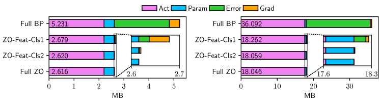
Figure 4: Memory usage breakdown of LeNet-5 (FP32; left: $B=32$, right: $B=256$).

Fig. 5 shows the memory cost of ElasticZO-INT8 as well as that of Full BP and Full ZO. In this case, we use Eqs. 13–15 to compute the memory cost required to train INT8 LeNet-5 on MNIST ($B=32,256$). Similar to the FP32 case (Fig. 4), Full ZO consumes the least amount of memory (1.8/1.6x less than Full BP for $B=32,256$) but has the lowest prediction accuracy (Table 1). On the other hand, ZO-Feat-Cls2 and ZO-Feat-Cls1 achieve a comparable accuracy to Full BP while maintaining nearly the same memory cost as Full ZO (0.052/1.4% and 0.26/4.1% more than Full ZO with $B=32,256$). As discussed in Sec. 4.4, FC and convolution layers need extra buffers to store intermediate accumulation results in 32-bit integers ${\bf\it a}_{l}^{\text{int32}},{\bf\it g}_{l}^{\text{int32}},{\bf\it e}_{l-1}^{\text{int32}}$ when computing activations, gradients, and errors. While the size of gradients and errors is substantially reduced in ElasticZO-INT8 and Full ZO, activations account for the largest portion of the entire memory usage (93.5% and 90.0% in ZO-Feat-Cls2 and ZO-Feat-Cls1 with $B=32$). Compared to the FP32 counterparts (Fig. 4), INT8 ZO methods (ZO-Feat-Cls1, ZO-Feat-Cls2, Full ZO) require 1.46–1.60x less memory, which is below an ideal case (4x) due to extra buffers ${\bf\it a}_{l}^{\text{int32}},{\bf\it g}_{l}^{\text{int32}},{\bf\it e}_{l-1}^{\text{int32}}$. While we assume that all necessary variables are allocated at once and not released during training, they can be dynamically allocated and deallocated as necessary to further optimize the memory usage, which is a future work.

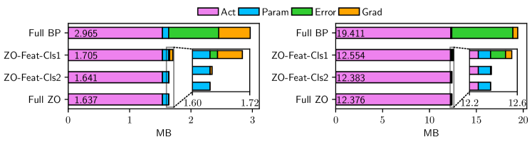
Figure 5: Memory usage breakdown of LeNet-5 (INT8; left: $B=32$, right: $B=256$).

Fig. 6 shows the memory usage when training PointNet on ModelNet40. The size of activations and errors is significantly larger than that of LeNet-5 (Fig. 4) and dominates the overall memory cost (99.4% and 99.3% in ZO-Feat-Cls2 and ZO-Feat-Cls1). As depicted in Fig. 1, PointNet extracts a high-dimensional local feature for each point using a stack of five FC layers, and then aggregates these per-point features into a global feature via max-pooling. The last FC layer in the feature extraction part produces an activation of size $(B,N,1024)$, with $B,N$ being the batch size and number of points ($N=1024$ in ModelNet40). While ElasticZO needs to keep gradients and errors of the last FC layers of the classification head, they are barely noticeable in Fig. 6 and do not significantly affect memory requirements (0.0087% and 0.12% for ZO-Feat-Cls2 and ZO-Feat-Cls1). As a result, ElasticZO almost halves the memory cost while achieving a comparable accuracy to Full BP (i.e., vanilla SGD) in the point cloud classification task as well.

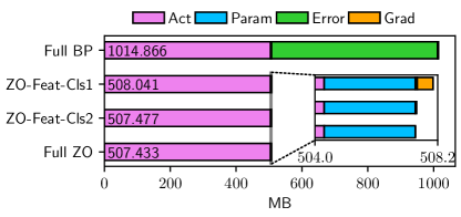
Figure 6: Memory usage breakdown of PointNet (FP32, $B=32$).

5.4 Execution Time

We evaluate the execution time of ElasticZO and ElasticZO-INT8 in comparison with Full ZO. Fig. 7 shows the results obtained on a Raspberry Pi Zero 2 board using our C++ implementation. We train the FP32 and INT8 LeNet-5 on MNIST for 100 epochs and measure the average execution time per epoch. Note that the breakdown follows the algorithms presented in Algs. 1–2 (e.g., Forward and ZO Update correspond to lines 6+8 and 5+7 in Alg. 1). Importantly, both ElasticZO and ElasticZO-INT8 maintain the training speed of Full ZO while significantly improving the accuracy. As expected, forward passes account for the largest portion of the wall-clock execution time and determine the overall performance (84.3–84.8% and 94.8–97.1% for ElasticZO and ElasticZO-INT8), whereas backward passes are almost negligible ($<$0.76% and $<$2.5%). This indicates that existing inference engines can be used to boost the performance of training with ElasticZO and ElasticZO-INT8. Besides, ElasticZO-INT8 is 1.38–1.42x faster than ElasticZO thanks to the use of low-precision arithmetic (FP32 SIMD instructions can be replaced by INT8 instructions that offer more parallelism). The parameter perturbation and update in ZO (ZO Perturb and ZO Update) are inherently memory-intensive and account for a non-negligible portion of the execution time (11.8–13.1%) in the FP32 case (left). On the other hand, they only account for 1.0–1.2% in the INT8 case (right), which can be attributed to 4x reduction of the parameter size and improved cache efficiency.

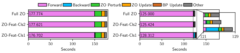
Figure 7: Execution time breakdown of the C++ implementation of Full ZO and ElasticZO on Raspberry Pi Zero 2 (left: FP32, right: INT8).

6 Conclusion

In this paper, we proposed ElasticZO and ElasticZO-INT8 as lightweight on-device learning methods that leverage memory-efficiency of ZO-based training and high accuracy of BP-based training. The key idea of ElasticZO is to employ BP for the last few layers and ZO for the remaining part. We devised a method to estimate quantized ZO gradients based on the integer cross-entropy loss, thereby allowing ElasticZO-INT8 to perform ZO-based training using only 8-bit integer arithmetic. We formulated the memory usage of ElasticZO and ElasticZO-INT8 to analyze their memory-efficiency. The evaluation on image and point cloud classification datasets demonstrated that, both ElasticZO and ElasticZO-INT8 achieve comparable prediction accuracy to Full BP by training only the last few FC layers with BP instead of ZO. They consumed nearly the same amount of memory and maintained the execution time as ZO methods, thereby significantly improving the trade-off between accuracy and training cost. On LeNet-5 and Fashion-MNIST, ElasticZO and ElasticZO-INT8 provided 5.2–9.5% and 6.4–10.7% higher accuracy than the vanilla ZO with a 0.072–0.17% and 0.052–0.26% memory overhead. ElasticZO-INT8 reduced the memory cost by 1.46–1.60x and execution time by 1.38–1.42x compared to ElasticZO without compromising the accuracy. Besides, ElasticZO and ElasticZO-INT8 are successfully applied to fine-tuning as well as training from scratch.

While being successful on simple DNN architectures and classification datasets, there is still an accuracy gap between ElasticZO and BP-based training that need to be addressed in a future work. In addition, it is an open problem to determine the number of layers trained by BP such that ElasticZO strikes the balance between accuracy and training cost. We also plan to apply ElasticZO to large-scale DNNs including language models and image diffusion models to evaluate the practicality of our approach. It is also possible to combine ElasticZO with PEFT techniques such as LoRA [49] and QLoRA [50].

References

- [1] David E. Rumelhart, Geoffrey E. Hinton, and Ronald J. Williams. Learning Representations by Back-propagating Errors. Nature, 323(6088):533–536, October 1986.
- [2] Yann LeCun, Bernhard Boser, John Denker, Donnie Henderson, R. Howard, Wayne Hubbard, and Lawrence Jackel. Handwritten Digit Recognition with a Back-Propagation Network. In Proceedings of the Advances in Neural Information Processing Systems (NIPS), pages 396–404, November 1989.
- [3] Y. LeCun, B. Boser, J. S. Denker, D. Henderson, R. E. Howard, and W. Hubbard. Backpropagation Applied to Handwritten Zip Code Recognition. Neural Computation, 1(4):541–551, December 1989.
- [4] John Duchi, Elad Hazan, and Yoram Singer. Adaptive Subgradient Methods for Online Learning and Stochastic Optimization. Journal of Machine Learning Research, 12(61):2121–2159, July 2011.
- [5] Diederik P. Kingma and Jimmy Ba. Adam: A Method for Stochastic Optimization. In Proceedings of the International Conference on Learning Representations (ICLR), pages 1–15, May 2015.
- [6] Sadhika Malladi, Tianyu Gao, Eshaan Nichani, Alex Damian, Jason D. Lee, Danqi Chen, and Sanjeev Arora. Fine-Tuning Large Language Models with Just Forward Passes. In Proceedings of the Advances in Neural Information Processing Systems (NeurIPS), pages 53038–53075, December 2023.
- [7] Sijia Liu, Pin-Yu Chen, Bhavya Kailkhura, Gaoyuan Zhang, Alfred O. Hero III, and Pramod K. Varshney. A Primer on Zeroth-Order Optimization in Signal Processing and Machine Learning: Principals, Recent Advances, and Applications. IEEE Signal Processing Magazine, 37(5):43–54, September 2020.
- [8] Yihua Zhang, Pingzhi Li, Junyuan Hong, Jiaxiang Li, Yimeng Zhang, Wenqing Zheng, Pin-Yu Chen, Jason D. Lee, Wotao Yin, Mingyi Hong, Zhangyang Wang, Sijia Liu, and Tianlong Chen. Revisiting Zeroth-Order Optimization for Memory-Efficient LLM Fine-Tuning: A Benchmark. In Proceedings of the International Conference on Machine Learning (ICML), pages 59173–59190, July 2024.
- [9] Pin-Yu Chen, Huan Zhang, Yash Sharma, Jinfeng Yi, and Cho-Jui Hsieh. ZOO: Zeroth Order Optimization Based Black-box Attacks to Deep Neural Networks without Training Substitute Models. In Proceedings of the ACM Workshop on Artificial Intelligence and Security (AISec), pages 15–26, November 2017.
- [10] Haishan Ye, Zhichao Huang, Cong Fang, Chris Junchi Li, and Tong Zhang. Hessian-Aware Zeroth-Order Optimization for Black-Box Adversarial Attack. arXiv preprint arXiv:1812.11377, December 2018.
- [11] Chun-Chen Tu, Paishun Ting, Pin-Yu Chen, Sijia Liu, Huan Zhang, Jinfeng Yi, Cho-Jui Hsieh, and Shin-Ming Cheng. AutoZOOM: Autoencoder-Based Zeroth Order Optimization Method for Attacking Black-Box Neural Networks. In Proceedings of the AAAI Conference on Artificial Intelligence (AAAI), pages 742–749, January 2019.
- [12] Yimeng Zhang, Yuguang Yao, Jinghan Jia, Jinfeng Yi, Mingyi Hong, Shiyu Chang, and Sijia Liu. How to Robustify Black-Box ML Models? A Zeroth-Order Optimization Perspective. In Proceedings of the International Conference on Learning Representations (ICLR), pages 1–15, April 2022.
- [13] Aochuan Chen, Yimeng Zhang, Jinghan Jia, James Diffenderfer, Jiancheng Liu, Konstantinos Parasyris, Yihua Zhang, Zheng Zhang, Bhavya Kailkhura, and Sijia Liu. DeepZero: Scaling up Zeroth-Order Optimization for Deep Model Training. In Proceedings of the International Conference on Learning Representations (ICLR), pages 1–22, May 2024.
- [14] Xiaoxing Wang, Wenxuan Guo, Jianlin Su, Xiaokang Yang, and Junchi Yan. ZARTS: On Zero-order Optimization for Neural Architecture Search. In Proceedings of the Advances in Neural Information Processing Systems (NeurIPS), pages 12868–12880, November 2022.
- [15] Lunchen Xie, Kaiyu Huang, Fan Xu, and Qingjiang Shi. ZO-DARTS: Differentiable Architecture Search with Zeroth-Order Approximation. In Proceedings of the IEEE International Conference on Acoustics, Speech and Signal Processing (ICASSP), pages 1–5, June 2023.
- [16] Sijia Liu, Jie Chen, Pin-Yu Chen, and Alfred Hero. Zeroth-Order Online Alternating Direction Method of Multipliers: Convergence Analysis and Applications. In Proceedings of the International Conference on Artificial Intelligence and Statistics (AISTATS), pages 288–297, April 2018.
- [17] Pengcheng He, Siyuan Lu, Xin Guan, Yibin Kang, and Qingjiang Shi. A Zeroth-Order Block Coordinate Gradient Descent Method For Cellular Network Optimization. In Proceedings of the International Symposium on Wireless Communication Systems (ISWCS), pages 1–6, October 2022.
- [18] Pengcheng He, Siyuan Lu, Fan Xu, Yibin Kang, Qi Yan, and Qingjiang Shi. A Parallel Zeroth-Order Framework for Efficient Cellular Network Optimization. IEEE Transactions on Wireless Communications, 23(11):17522–17538, November 2024.
- [19] Zhiwei Tang, Dmitry Rybin, and Tsung-Hui Chang. Zeroth-Order Optimization Meets Human Feedback: Provable Learning via Ranking Oracles. In Proceedings of the International Conference on Learning Representations (ICLR), pages 1–31, May 2024.
- [20] Qining Zhang and Lei Ying. Zeroth-Order Policy Gradient for Reinforcement Learning from Human Feedback without Reward Inference. arXiv preprint arXiv:2409.17401, September 2024.
- [21] Tanmay Gautam, Youngsuk Park, Hao Zhou, Parameswaran Raman, and Wooseok Ha. Variance-reduced Zeroth-Order Methods for Fine-Tuning Language Models. arXiv preprint arXiv:2404.08080, April 2024.
- [22] Shuoran Jiang, Qingcai Chen, Youchen Pan, Yang Xiang, Yukang Lin, Xiangping Wu, Chuanyi Liu, and Xiaobao Song. ZO-AdaMU Optimizer: Adapting Perturbation by the Momentum and Uncertainty in Zeroth-order Optimization. In Proceedings of the AAAI Conference on Artificial Intelligence (AAAI), pages 18363–18371, February 2024.
- [23] Yong Liu, Zirui Zhu, Chaoyu Gong, Minhao Cheng, Cho-Jui Hsieh, and Yang You. Sparse MeZO: Less Parameters for Better Performance in Zeroth-Order LLM Fine-Tuning. arXiv preprint arXiv:2402.15751, February 2024.
- [24] Wentao Guo, Jikai Long, Yimeng Zeng, Zirui Liu, Xinyu Yang, Yide Ran, Jacob R. Gardner, Osbert Bastani, Christopher De Sa, Xiaodong Yu, Beidi Chen, and Zhaozhuo Xu. Zeroth-Order Fine-Tuning of LLMs with Extreme Sparsity. arXiv preprint arXiv:2406.02913, June 2024.
- [25] Sijia Liu, Pin-Yu Chen, Xiangyi Chen, and Mingyi Hong. signSGD via Zeroth-Order Oracle. In Proceedings of the International Conference on Learning Representations (ICLR), pages 1–24, May 2019.
- [26] Yurii Nesterov and Vladimir Spokoiny. Random Gradient-Free Minimization of Convex Functions. Foundations of Computational Mathematics, 17(1):527–566, April 2017.
- [27] Saeed Ghadimi and Guanghui Lan. Stochastic First- and Zeroth-Order Methods for Nonconvex Stochastic Programming. SIAM Journal on Optimization, 23(4):2341–2368, December 2013.
- [28] Xiangru Lian, Huan Zhang, Cho-Jui Hsieh, Yijun Huang, and Ji Liu. A Comprehensive Linear Speedup Analysis for Asynchronous Stochastic Parallel Optimization from Zeroth-Order to First-Order. In Proceedings of the Advances in Neural Information Processing Systems (NeurIPS), pages 1–9, December 2016.
- [29] Sijia Liu, Bhavya Kailkhura, Pin-Yu Chen, Paishun Ting, Shiyu Chang, and Lisa Amini. Zeroth-Order Stochastic Variance Reduction for Nonconvex Optimization. In Proceedings of the Advances in Neural Information Processing Systems (NeurIPS), pages 1–11, December 2018.
- [30] Kaiyi Ji, Zhe Wang, Yi Zhou, and Yingbin Liang. Improved Zeroth-Order Variance Reduced Algorithms and Analysis for Nonconvex Optimization. In Proceedings of the International Conference on Machine Learning (ICML), pages 3100–3109, June 2019.
- [31] Sashank J. Reddi, Ahmed Hefny, Suvrit Sra, Barnabas Poczos, and Alex Smola. Stochastic Variance Reduction for Nonconvex Optimization. In Proceedings of the International Conference on Machine Learning (ICML), pages 314–323, June 2016.
- [32] Jeremy Bernstein, Yu-Xiang Wang, Kamyar Azizzadenesheli, and Animashree Anandkumar. signSGD: Compressed Optimisation for Non-Convex Problems. In Proceedings of the International Conference on Machine Learning (ICML), pages 560–569, July 2018.
- [33] Feihu Huang, Shangqian Gao, Jian Pei, and Heng Huang. Accelerated Zeroth-Order and First-Order Momentum Methods from Mini to Minimax Optimization. The Journal of Machine Learning Research, 23(36):1–70, February 2022.
- [34] Xiangyi Chen, Sijia Liu, Kaidi Xu, Xingguo Li, Xue Lin, Mingyi Hong, and David Cox. ZO-AdaMM: Zeroth-Order Adaptive Momentum Method for Black-Box Optimization. In Proceedings of the Advances in Neural Information Processing Systems (NeurIPS), pages 7204–7215, December 2019.
- [35] Yifan Yang, Kai Zhen, Ershad Banijamal, Athanasios Mouchtaris, and Zheng Zhang. AdaZeta: Adaptive Zeroth-Order Tensor-Train Adaption for Memory-Efficient Large Language Models Fine-Tuning. In Proceedings of the Conference on Empirical Methods in Natural Language Processing (EMNLP), pages 977–995, November 2024.
- [36] Xinyu Tang, Ashwinee Panda, Milad Nasr, Saeed Mahloujifar, and Prateek Mittal. Private Fine-tuning of Large Language Models with Zeroth-order Optimization. arXiv preprint arXiv:2401.04343, January 2024.
- [37] Zhen Qin, Daoyuan Chen, Bingchen Qian, Bolin Ding, Yaliang Li, and Shuiguang Deng. Federated Full-Parameter Tuning of Billion-Sized Language Models with Communication Cost under 18 Kilobytes. In Proceedings of the International Conference on Machine Learning (ICML), pages 41473–41497, July 2024.
- [38] Zhenqing Ling, Daoyuan Chen, Liuyi Yao, Yaliang Li, and Ying Shen. On the Convergence of Zeroth-Order Federated Tuning for Large Language Models. In Proceedings of the ACM SIGKDD Conference on Knowledge Discovery and Data Mining (KDD), pages 1827–1838, August 2024.
- [39] Yequan Zhao, Hai Li, Ian Young, and Zheng Zhang. Poor Man’s Training on MCUs: A Memory-Efficient Quantized Back-Propagation-Free Approach. arXiv preprint arXiv:2411.05873, November 2024.
- [40] Dan Peng, Zhihui Fu, and Jun Wang. PocketLLM: Enabling On-Device Fine-Tuning for Personalized LLMs. In Proceedings of the Workshop on Privacy in Natural Language Processing (PrivateNLP), pages 91–96, August 2024.
- [41] J.C. Spall. Multivariate Stochastic Approximation using a Simultaneous Perturbation Gradient Approximation. IEEE Transactions on Automatic Control, 37(3):332–341, March 1992.
- [42] Maolin Wang, Seyedramin Rasoulinezhad, Philip H. W. Leong, and Hayden K.-H. So. NITI: Training Integer Neural Networks Using Integer-Only Arithmetic. IEEE Transactions on Parallel and Distributed Systems (TPDS), 33(11):3249–3261, November 2022.
- [43] Yann Lecun, Léon Bottou, Yoshua Bengio, and Patrick Haffner. Gradient-Based Learning Applied to Document Recognition. Proceedings of the IEEE, 86(11):2278–2324, November 1998.
- [44] Han Xiao, Kashif Rasul, and Roland Vollgraf. Fashion-MNIST: a Novel Image Dataset for Benchmarking Machine Learning Algorithms. arXiv preprint arXiv:1708.07747, September 2017.
- [45] Zhirong Wu, Shuran Song, Aditya Khosla, Fisher Yu, Linguang Zhang, Xiaoou Tang, and Jianxiong Xiao. 3D ShapeNets: A Deep Representation for Volumetric Shapes. In Proceedings of the IEEE Conference on Computer Vision and Pattern Recognition (CVPR), pages 1912–1920, June 2015.
- [46] Charles R. Qi, Hao Su, Kaichun Mo, and Leonidas J. Guibas. PointNet: Deep Learning on Point Sets for 3D Classification and Segmentation. In Proceedings of the IEEE Conference on Computer Vision and Pattern Recognition (CVPR), pages 652–660, July 2017.
- [47] Vihari Piratla, Praneeth Netrapalli, and Sunita Sarawagi. Efficient Domain Generalization via Common-Specific Low-Rank Decomposition. In Proceedings of the International Conference on Machine Learning (ICML), pages 7728–7738, July 2020.
- [48] Honoka Anada, Sefutsu Ryu, Masayuki Usui, Tatsuya Kaneko, and Shinya Takamaeda-Yamazaki. PRIOT: Pruning-Based Integer-Only Transfer Learning for Embedded Systems. IEEE Embedded Systems Letters, October 2024. Early Access.
- [49] Edward Hu, Yelong Shen, Phillip Wallis, Zeyuan Allen-Zhu, Yuanzhi Li, Shean Wang, Lu Wang, and Weizhu Chen. LoRA: Low-Rank Adaptation of Large Language Models. In Proceedings of the International Conference on Learning Representations (ICLR), pages 1–13, April 2022.
- [50] Tim Dettmers, Artidoro Pagnoni, Ari Holtzman, and Luke Zettlemoyer. QLoRA: Efficient Finetuning of Quantized LLMs. In Proceedings of the Advances in Neural Information Processing Systems (NeurIPS), pages 10088–10115, December 2023.