Making school choice lotteries transparent

Abstract

Lotteries are commonly employed in school choice to fairly resolve priority ties; however, current practices leave students uninformed about their lottery outcomes when submitting preferences. This paper advocates for revealing lottery results prior to preference submission. When preference lists are constrained in length, revealing lotteries can reduce uncertainties and enable informed decision-making regarding the selection of schools to rank. Through three stylized models, we demonstrate the benefits of lottery revelation in resolving conflicting preferences, equalizing opportunities among students with varying outside options, and alleviating the neighborhood school bias. Our findings are further supported by a laboratory experiment.

Keywords: School choice; lottery; uncertainty; neighborhood school bias; laboratory experiment

JEL Classification: C78, C91, D71, I20

1 Introduction

Many cities worldwide use centralized school admission mechanisms and assign school priorities to students based on broad criteria, including geographic proximity, demographic characteristics, and other factors. Priority ties frequently occur within these systems. Popular mechanisms (e.g., deferred acceptance), which require strict priority orders for input, often resort to lotteries to resolve these ties to address fairness concerns. Despite crucial roles played by lotteries in determining students’ assignments, in current practices, lottery results are not revealed to students before they submit preferences. To our knowledge, this issue has been overlooked in previous school choice literature, presumably for two reasons. First, strict priorities are assumed in many papers at the outset, thereby eliminating the need for lotteries. Second, students are assumed to report complete preference lists in many papers, precluding their need for lottery information, provided that strategy-proof mechanisms are employed. However, in circumstances where preference lists are constrained in length, which are common in practice, no mechanisms can be truly strategy-proof, as students must strategize when determining which schools to rank, resulting in the thorny issue of unmatch. In NYC, while students can rank up to twelve schools, 7% (around 5,000 students) remained unmatched after the main round of the match during the years 2021 and 2022. In certain districts, such as Manhattan district (D2), the unmatch rate can reach as high as 18%. Consequently, the unmatch rate emerges as a metric that policymakers aim to reduce.

This paper advocates for a “revealing” policy wherein lotteries are drawn and revealed to students prior to their submission of preferences, contrasting it with the currently used “covering” policy, whereby students are uninformed about their lotteries before submitting preferences. To illustrate the differing consequences of the two policies, consider two students $i$ and $j$ who compete for two schools A and B, each with a single seat. Both students prefer A over B and they are in priority ties for both schools. A single lottery is used to break the ties. Students are limited to reporting only one school. Under the covering policy, provided that both students value A sufficiently higher than B, both will report A. This is a rational choice, despite their full awareness of the risk of remaining unmatched. In contrast, under the revealing policy, students can more effectively coordinate their strategies upon learning their lottery numbers; the student favored by the lottery outcome will report A and the other will report B. Consequently, both students will always be matched, and ex ante each still has an equal chance of being admitted to A.

To formally demonstrate the benefit of the revealing policy versus the covering policy, we compare them in three variants of the canonical model of Abdulkadiroglu, Che and Yasuda (2011). In their model, students have common ordinal preferences over schools, but may have different cardinal utilities, which are private information. Schools do not prioritize students and rely solely on a lottery to rank students. The deferred acceptance (DA) mechanism is used to determine the matching. This extreme priority structure and conflicting preference setup amplify the role of lotteries and simplify our analysis.

Our first model deviates from Abdulkadiroglu, Che and Yasuda (2011) by imposing a restriction on the number of schools that students may report. Therefore, students need to decide which schools to rank. The revealing policy effectively resolves uncertainties for students by essentially informing them of their attainable schools via lottery numbers, resulting in a matching outcome equivalent to that produced by DA with complete preference lists. Consequently, every student is matched. From an interim perspective (after utilities are realized but before the lottery is drawn), every student has an equal chance of attending each school. In contrast, under the covering policy, students need to strategize. For certain realized utilities, students may concentrate their preference submissions on a subset of schools, resulting in wasted seats at other schools and leaving some students unmatched. From an interim perspective, every student faces a positive probability of remaining unmatched, and from an ex-ante perspective (before utilities and the lottery are drawn), students receive an equal random assignment that is first-order stochastically dominated by that obtained under the revealing policy. Overall, the first model demonstrates the benefit of the revealing policy in resolving students’ conflicting preferences.

Our second model diverges from the first one by assuming that some students have outside options while the others do not. Prevalently, students participating in the same school choice system often have access to different outside options (e.g., private schools, options in parallel choice systems). This raises the concern that unequal outside options can create inequity among students. Our analysis supports this concern for the covering policy. With outside options as a backup, relevant students report popular schools more frequently than in the first model. As a response, students without outside options strategically avoid reporting popular schools. Thus, students with outside options gain an undue advantage over their peers. In contrast, the revealing policy levels the playing field by providing all students equal opportunities to enter popular schools.

Our third model modifies the first one by assuming that every school prioritizes a subset of students based on neighborhood proximity, ranking them above others, while still resolving ties within the same group through a single lottery. This model addresses the complexities associated with nontrivial priorities in practice, of which neighborhood priority is a prominent example. The existence of neighborhood priorities complicates our previous analysis. Consider a student who, upon learning his lottery number, applies to a school where he lacks neighborhood priority. In the first model, his lottery number informs him of his ranking among all students for all schools, but now he faces uncertainty regarding the number of students who receive worse lottery numbers than his yet have neighborhood priority for the school in question. Consequently, the ability to make informed decisions requires him to calculate probabilities involving complicated combinatorics. In practice, policymakers may provide statistics about the realized lottery distribution to reduce such uncertainties for students. Our model offers an additional insight that this issue will be mitigated in large markets due to the law of large numbers. In a model with a continuum of students and a finite number of schools, we show that the revealing policy mitigates the so-called “neighborhood school bias” by resolving the uncertainty caused by lotteries, whereas the covering policy tends to exacerbate this uncertainty, leading students to be more inclined to select their neighborhood schools.

Another potential advantage of the revealing policy is that, when it has been used in a market for years and the market fundamentals (including the distribution of student preferences and school priorities) do not change much over years, the cutoff lottery numbers for schools will tend to stabilize. Then, students may rely on historical cutoff data and their current lottery numbers to estimate their chances for different schools, significantly simplifying their strategies. Although this argument seems to be new for lottery-based school choice, it has been verified in test-based admission systems in countries such as China and Turkey, and the theoretical insight has been conveyed by Azevedo and Leshno (2016) who show that a continuum school choice model generically has a unique stable matching, which is the limit of stable matching in large finite markets.

We complement our theoretical models with a laboratory experiment. To align more closely with real-world scenarios, we design a school choice market with neighborhood priorities and constrained preference lists, and implement a between-subject design to compare the market performance under the two policies. The experimental results indicate that revealing lotteries constitutes a superior policy, as it yields a significantly higher match rate, reduced neighborhood school bias, decreased segregation levels, and enhanced average student welfare compared to the covering policy. Students are able to make more informed decisions by mostly reporting schools where they have realistic chances of acceptance, whereas under the covering policy, they tend to report unattainable schools more frequently.

It is noteworthy that during the preparation of this paper, NYC adopted the revealing policy for the 2022-2023 season. Initially, NYC refused to reveal lottery numbers to parents. However, following a parent-led campaign under the New York State’s Freedom of Information Law, NYC first agreed to reveal lotteries upon request after admissions and finally decided to disclose lotteries before applications. The empirical implications of this policy shift represent an exciting area for future research. NYC continues to progress toward providing more comprehensive information about lotteries. For instance, it still withholds historical cutoff data. Using a crowdsourced survey, Marian (2023) estimates school cutoffs and demonstrates their positive impact on reducing the unmatch rate in subsequent years among the survey participants.

Related literature

Our models are built on the work of Abdulkadiroglu, Che and Yasuda (2011), who compare the Boston mechanism (BM) and DA under unconstrained preference lists and the covering policy. Differently, our study focuses on comparing the two lottery policies under constrained preference lists, given DA is employed. Our insights also differ. In their model, the welfare superiority of BM over DA arises from students’ strategic behavior in response to the uncertainties associated with tie-breaking. However, the experiments of Featherstone and Niederle (2016) suggest that real-life students are unlikely to reach the non-truth-telling equilibrium of BM. Conversely, in our model, the benefits of the revealing policy stem from students’ straightforward behavior after learning their lottery outcomes. Thus, we expect that such benefits are likely to be realized in practice.

Our second model is related to Akbarpour et al. (2022) who add unequal outside options to the model of Abdulkadiroglu, Che and Yasuda (2011) and similarly show that students with outside options gain an undue advantage in manipulable mechanisms. They consider complete preference lists and the covering policy, which allows them to use a proof method similar to that of Abdulkadiroglu, Che and Yasuda (2011) to compare students’ welfare between manipulable and strategy-proof mechanisms. In contrast, we consider constrained preference lists and emphasize the role of the revealing policy in leveling the playing field.

Additionally, there exists a body of literature that compares single lotteries versus multiple lotteries for tie-breaking (e.g., Abdulkadiroğlu, Pathak and Roth (2009); Pathak and Sethuraman (2011); Ashlagi and Nikzad (2020); Arnosti (2023)). Single lotteries are more frequently employed in practice (e.g., in NYC). While our paper operates under the assumption of a single lottery, the main insight carries over to multiple lotteries. However, in the context of multiple lotteries, students must navigate more complex information, which leads us to believe that a single lottery is superior in this regard.

2 Three Models

2.1 Resolving conflicting preferences

We present the setup of Abdulkadiroglu, Che and Yasuda (2011). A finite set of students $I=\{i_{1},\cdots,i_{n}\}$ seeks admission to a finite set of schools $S=\{s_{1},\cdots,s_{m}\}$. Each school $s$ has capacity $q_{s}\in\mathbb{N}$. We assume that $\sum_{s\in S}q_{s}=|I|$; that is, the school seats are exactly enough to admit all students. Each student $i$ has a utility vector $\mathbf{v}^{i}=(v^{i}_{1},v^{i}_{2},\ldots,v^{i}_{m})$ where $v^{i}_{k}\in[0,1]$ denotes $i$’s utility of attending school $s_{k}$. Each $\mathbf{v}^{i}$ is independently drawn from a finite set $\mathcal{V}=\{(v_{k})_{k=1}^{m}\in[0,1]^{m}:v_{1}>v_{2}>\cdots>v_{m}\}$ with probability $f(\mathbf{v}^{i})$. Therefore, students have identical ordinal preferences: $s_{1}\succ s_{2}\succ s_{3}\ldots\succ s_{m}$. Students know their own cardinal utilities but not the others’, except for the underlying probability distribution $f$. All students are in priority ties for all schools. A single lottery, represented by a one-to-one mapping $\pi:I\rightarrow\{1,2,\ldots,n\}$, is drawn uniformly at random to break ties. If $\pi(i)<\pi(j)$, it means that $i$ is ranked above $j$ in the lottery.

A matching is a function $\mu:I\rightarrow S\cup\{\emptyset\}$ such that, for each school $s$, $|\mu^{-1}(s)|\leq q_{s}$. For any student $i$, if $\mu(i)=\emptyset$, it means that $i$ is unmatched.

We use $\ell$ to denote the length of the rank-order list (ROL) and assume that $\ell<m$. We denote the student-proposing DA in our model by $\text{DA}^{\ell}$ to emphasize the constrained ROL. The definition of DA can be found in textbooks such as Roth and Sotomayor (1992).

Figure 1: Timeline of the revealing policy

We compare two policies regarding the disclosure of lottery information. Under the revealing policy, students are informed of their lottery number before submitting ROLs, while under the covering policy, students remain uninformed about their lottery outcome before submitting ROLs. Figure 1 shows the timeline of the school choice game under the revealing policy: students’ utilities are first realized; then, the lottery is drawn and revealed to the students, each learning only his own lottery number; students then submit their ROLs; finally, the matching is generated.

Our analysis compares the two policies at different stages of the game. Ex-ante refers to the timing before students’ utilities are realized. Interim refers to the timing after students’ utilities are realized but before the lottery is drawn. For individual students, interim also denotes the timing when they only know their own utilities (but do not know the others’ and the lottery outcome). Ex-post refers to the timing after the lottery has been drawn and students have submitted their ROLs.

We first show that the revealing policy simplifies students’ strategies by effectively informing them of their best attainable schools.

Lemma 1.

Under the revealing policy, for any realized utilities and any drawn lottery, in the unique Bayesian Nash equilibrium, the top $q_{s_{1}}$ students in the lottery must rank $s_{1}$ first in their ROLs and are admitted to $s_{1}$; the next $q_{s_{2}}$ students in the lottery must essentially rank $s_{2}$ first in their ROLs and are admitted to $s_{2}$; the next $q_{s_{3}}$ students in the lottery must essentially rank $s_{3}$ first in their ROLs and are admitted to $s_{3}$; and so on.

Proof.

Under the revealing policy, if a student knows that his lottery number is among the top $q_{s_{1}}$, he must rank $s_{1}$ first in his ROL and be admitted to $s_{1}$. Given this, if a student knows that his lottery number is among the next $q_{s_{2}}$ below the top $q_{s_{1}}$, he knows that the top $q_{s_{1}}$ students must be admitted to $s_{1}$ and, therefore, $s_{2}$ is his best attainable school. So he must rank $s_{2}$ first (or only below $s_{1}$) in his ROL and be admitted to $s_{2}$. Similarly, the next $q_{s_{3}}$ students in the lottery must essentially rank $s_{3}$ first and be admitted to $s_{3}$. The result holds inductively for all other students. ∎

From an ex-post perspective, provided that the same lottery is drawn, the result of constrained DA with the revealing policy coincides with the outcome of unconstrained DA where all students report complete and true preferences.

From an interim perspective, since the lottery is drawn uniformly at random, students have equal probabilities of receiving each lottery number, implying that they have equal chances of attending each school. So, each student effectively receives an equal division assignment $(\frac{q_{s}}{n}\cdot s)_{s\in S}$. This result also holds from an ex-ante perspective.

Next, we analyze the covering policy, where students cannot base their strategies on their lottery numbers. Let $\mathcal{L}^{\ell}$ denote the set of all possible ROLs that rank no more than $\ell$ schools. A (mixed) strategy is a mapping $\sigma:\mathcal{V}\rightarrow\Delta(\mathcal{L}^{\ell})$, where $\Delta(\mathcal{L}^{\ell})$ denotes the set of probability distributions on $\mathcal{L}^{\ell}$. For any utility vector $\mathbf{v}^{i}$, $\sigma(\mathbf{v}^{i})$ is a strategy in which $i$ reports $L\in\mathcal{L}^{\ell}$ with probability $\sigma(\mathbf{v}^{i})(L)$.

We focus on symmetric Bayesian Nash equilibrium (BNE) in which students with identical utilities play the same strategies. Let $\sigma^{*}$ denote such an equilibrium. Then, for any realized utilities $\mathbf{v}=(\mathbf{v}^{i})_{i\in I}$, each student $i$ plays the strategy $\sigma^{*}(\mathbf{v}^{i})$. Although we do not characterize $\sigma^{*}$, we know that, for any $L\in\mathcal{L}^{\ell}$ such that $\sigma^{*}(\mathbf{v}^{i})(L)>0$, at least $m-\ell$ schools are not listed in $L$. Therefore, if all students have equal cardinal utilities $\mathbf{v}^{i}$, which occurs with positive probability, with probability $\sum_{L\in\mathcal{L}^{\ell}}[\sigma^{*}(\mathbf{v}^{i})(L)]^{n}$, at least $m-\ell$ schools are not reported by any student, resulting in a number of unmatched students at least equal to the total capacity of those schools. More generally, as long as there is a positive probability that some school $s$ is not reported by any student, at least $q_{s}$ students will be unmatched. From an interim perspective, every student believes that there is a positive probability that the others have identical utilities to his, so he has a positive probability of being unmatched. From an ex-ante perspective, because students are symmetric, they must receive equal random assignments in which they have positive probabilities to be unmatched. So, the random assignment must be first-order stochastically dominated by the equal division assignment $(\frac{q_{s}}{n}\cdot s)_{s\in S}$, which is the outcome under the revealing policy. Thus, we present the following result without proof.

Proposition 1.

Under the revealing policy: (1) From an ex-post perspective, the outcome of $\text{DA}^{\ell}$ coincides with the dominant strategy outcome of DA with unconstrained ROL. In particular, every student is matched; (2) From an interim (and ex-ante) perspective, every student receives the same random assignment $(\frac{q_{s}}{n}\cdot s)_{s\in S}$.

Under the covering policy: (1) With a positive probability, the ex-post matching includes unmatched students whose number is at least equal to the total capacity of $m-\ell$ schools; (2) From an interim perspective, each student believes that he has a positive probability of being unmatched; (3) From an ex-ante perspective, each student obtains an equal random assignment that is first-order stochastically dominated by that under the revealing policy.

We provide an example in which students’ equilibrium strategies are characterized.

Example 1.

There are three students $\{1,2,3\}$ and three schools $\{s_{1},s_{2},s_{3}\}$. Each school has one seat and each student can report one school ($\ell=1$). There are two types of students’ utilities $\{\mathbf{v},\mathbf{v}^{\prime}\}$, which follow the distribution $f(\mathbf{v})=2/3$ and $f(\mathbf{v}^{\prime})=1/3$:

	$\mathbf{v}$	$\mathbf{v}^{\prime}$
$s_{1}$	$0.6$	$0.46$
$s_{2}$	$0.3$	$0.44$
$s_{3}$	$0.1$	$0.1$

Under the covering policy, there is a unique symmetric BNE in which type-$\mathbf{v}$ students report $s_{1}$ and type-$\mathbf{v}^{\prime}$ students report $s_{2}$. To verify this is an equilibrium, for any student $i$, if the others follow the equilibrium strategy, then the probability of being admitted to each school by reporting that school is:

$$s_{1}: \quad\dfrac{2}{3}\times\dfrac{2}{3}\times\dfrac{1}{3}+2\times\dfrac{2}{3}\times\dfrac{1}{3}\times\dfrac{1}{2}+\dfrac{1}{3}\times\dfrac{1}{3}\times 1 =\dfrac{13}{27}$$

$$s_{2}: \quad\dfrac{2}{3}\times\dfrac{2}{3}\times 1+2\times\dfrac{2}{3}\times\dfrac{1}{3}\times\dfrac{1}{2}+\dfrac{1}{3}\times\dfrac{1}{3}\times\dfrac{1}{3} =\dfrac{19}{27}$$

$$s_{3}: =1$$

So, if $i$’s utility is $\mathbf{v}$, his optimal strategy is to report $s_{1}$; if his utility is $\mathbf{v}^{\prime}$, his optimal strategy is to report $s_{2}$. In this equilibrium, $s_{3}$ is always empty, and the number of unmatched students is at least one. From an ex-ante perspective, every student obtains the random assignment $(\frac{26}{81}s_{1},\frac{19}{81}s_{2},\frac{36}{81}\emptyset)$, which is first-order stochastically dominated by the equal division assignment $(\frac{1}{3}s_{1},\frac{1}{3}s_{2},\frac{1}{3}s_{3})$ under the revealing policy.

Students also obtain strictly higher interim expected utilities under the revealing policy than under the covering policy. Under the revealing policy, every student obtains an expected utility $\frac{9}{27}$ regardless of his utility type, while under the covering policy, every type-$\mathbf{v}$ student obtains an expected utility $\frac{7.8}{27}$ and every type-$\mathbf{v}^{\prime}$ student obtains an expected utility $\frac{8.36}{27}$.

2.2 Leveling the playing field under unequal outside options

Based on the first model, we now assume that a subset of students $I^{\prime}\subsetneq I$ has an outside option $s^{*}$, which has enough capacity to accommodate all students in $I^{\prime}$ and is ranked among all schools as follows: $s_{1}\succ\cdots\succ s_{x}\succ s^{*}\succ s_{x+1}\succ\cdots\succ s_{m}$, for some $x\leq\ell$. The students in $I\backslash I^{\prime}$ do not have outside options. By assuming that $s^{*}$ is better than $s_{x+1}$, we simplify the strategies of students in $I^{\prime}$ under the covering policy: they have a weakly dominant strategy of reporting the truncated ROL $(s_{1},s_{2},\ldots,s_{x})$, and if they are not admitted to any school in that ROL, they attend $s^{*}$. In general, as long as $s^{*}$ is better than $s_{m}$, students in $I^{\prime}$ will report only schools better than $s^{*}$ in their ROLs, leading to an advantage relative to $I\backslash I^{\prime}$. Our assumption makes this insight transparent.

Under the revealing policy, our previous analysis is still valid. The only difference is that the students in $I^{\prime}$ never compete with $I\backslash I^{\prime}$ for any school worse than $s^{*}$. This means that students in $I\backslash I^{\prime}$ have higher probabilities of attending any school worse than $s^{*}$ than in the first model. For each school $s$ better than $s^{*}$, from an interim perspective, each student is admitted to $s$ with equal probability $\frac{q_{s}}{n}$.

Under the covering policy, students in $I^{\prime}$ always report the truncated ROL $(s_{1},s_{2},\ldots,s_{x})$. To study the impacts of unequal outside options, we examine how students might change their strategies when we move from the first model to the second. If, in the equilibrium of the first model, students in $I^{\prime}$ always report $(s_{1},s_{2},\ldots,s_{x})$ as the top $x$ schools in their ROLs, then, because all students are symmetric in the first model, all students must always report $(s_{1},s_{2},\ldots,s_{x})$ as the top $x$ schools in their ROLs. In this case, under the covering policy, all students are assigned to each of $s_{1},s_{2},\ldots,s_{x}$ with equal probability as under the revealing policy. To rule out this nongeneric case, we assume the above situation is not an equilibrium in the first model. This means that when we move from the first model to the second, students in $I^{\prime}$ change their strategies by reporting $s_{1},s_{2},\ldots,s_{x}$ with higher probabilities (the probability is strictly higher for at least one school and at least one utility type). As a response, students in $I\backslash I^{\prime}$ might change their strategies and, generally, will report $s_{1},s_{2},\ldots,s_{x}$ with lower probabilities compared to the first model. Although we do not characterize these changes, we can draw the following conclusion, which demonstrates the advantage of the students in $I^{\prime}$ under the covering policy.

Proposition 2.

(1) Under the covering policy, from an ex-ante perspective, there exists a school $s_{y}$ weakly better than $s_{x}$ such that every $i\in I^{\prime}$ is admitted to every $s\in\{s_{1},s_{2},\ldots,s_{y}\}$ with weakly higher probability and to $s_{y}$ with strictly higher probability compared to the revealing policy; (2) The revealing policy levels the playing field in the sense that, from an interim (and ex-ante) perspective, every student is admitted to every $s\in\{s_{1},s_{2},\ldots,s_{x}\}$ with equal probability $\frac{q_{s}}{n}$.

Proof.

Since the second part holds similarly to the first model, we only prove the first part. Given that every $i\in I^{\prime}$ must report the truncated ROL $(s_{1},s_{2},\ldots,s_{x})$ under the covering policy, they must be assigned to $s_{1}$ with a probability weakly higher than $\frac{q_{s_{1}}}{n}$. If the probability is strictly higher than $\frac{q_{s_{1}}}{n}$, then, letting $s_{y}=s_{1}$, we are done. If the probability equals $\frac{q_{s_{1}}}{n}$, every $j\in I\backslash I^{\prime}$ must also report $s_{1}$ as the first choice in their ROLs. Then, every $i\in I^{\prime}$ must be assigned to $s_{2}$ with a probability weakly higher than $\frac{q_{s_{2}}}{n}$, and the probability equals $\frac{q_{s_{2}}}{n}$ if and only if every $j\in I\backslash I^{\prime}$ also reports $s_{2}$ as the second choice in their ROLs. Inductively, every $i\in I^{\prime}$ is assigned to every $s\in\{s_{1},s_{2},\ldots,s_{x}\}$ with a probability $\frac{q_{s}}{n}$ if and only if every $j\in I\backslash I^{\prime}$ reports $(s_{1},s_{2},\ldots,s_{x})$ as the top $x$ schools in their ROLs, which is ruled out by our assumption. So, there must exist a school $s_{y}$ weakly better than $s_{x}$ such that every $i\in I^{\prime}$ is assigned to $s_{y}$ with a probability strictly higher than $\frac{q_{s_{y}}}{n}$. ∎

In the following, we discuss how the students in Example 1 change their strategies compared to the first model when one of them has an outside option that is only worse than $s_{1}$. In the example, the student with an outside option is better off under the covering policy than under the revealing policy, but not all of the others are worse off.

Example 2.

Suppose that student $1$ in Example 1 has an outside option $s^{*}$ such that $s_{1}\succ s^{*}\succ s_{2}\succ s_{3}$. Then, under the covering policy, student $1$ must report $s_{1}$. Given this, in the unique symmetric BNE, among the other two students, every type-$\mathbf{v}$ student plays a mixed strategy in which he reports $s_{1}$ with probability $0.9$ and reports $s_{2}$ with probability $0.1$; every type-$\mathbf{v}^{\prime}$ student surely reports $s_{2}$. Note that type-$\mathbf{v}$ students now report $s_{1}$ with a lower probability compared to Example 1.

In the above equilibrium under the covering policy, from an interim view, $1$ is assigned to $s_{1}$ with probability $0.52$, which is higher than the counterpart probability $1/3$ under the revealing policy and also higher than the counterpart probability for type-$\mathbf{v}$ students under the covering policy in Example 1 ($\frac{13}{27}\approx 0.48$). In contrast, among the other two students, every type-$\mathbf{v}$ student is assigned to $s_{1}$ with probability $0.9\times 0.4=0.36$ and to $s_{2}$ with probability $0.1\times 0.8=0.08$, which is first-order stochastically dominated by the probability of being assigned to $s_{1}$ in Example 1 ($\frac{13}{27}\approx 0.48$). So type-$\mathbf{v}$ students are worse off compared to Example 1. Every type-$\mathbf{v}^{\prime}$ student, however, is better off. He is assigned to $s_{2}$ with probability $0.8$ in this example, which is higher than the counterpart probability in Example 1 ($\frac{19}{27}\approx 0.70$).

2.3 Mitigating the neighborhood school bias

In the former two models, we assume that all students have equal priorities for all schools. In practice, however, schools often use nontrivial priorities, and neighborhood is one of the most frequently observed priority policies. This subsection adds neighborhood priority to the first model and assumes a continuum of students.

Formally, there is a mass 1 of students and finite schools $S=\{s_{1},\cdots,s_{m}\}$. The capacity of each school $s$ is $q_{s}\in(0,1)$, and $\sum_{s\in S}q_{s}=1$. A mass $n_{s}\in(0,q_{s})$ of students, the set of which denoted by $I_{s}$, live in the neighborhood of school $s$. Since $n_{s}<q_{s}$, each school has additional capacity to admit students outside its neighborhood. Each student lives in the neighborhood of at most one school, and a mass $1-\sum_{s\in S}n_{s}$ of students do not live in any neighborhood. Each school $s$ ranks the students in $I_{s}$ above the others, with priority ties broken by a randomly drawn lottery represented by a one-to-one mapping $\pi:I\rightarrow[0,1]$. Students’ ordinal preferences and cardinal utilities are assumed as in the first model.

Under the revealing policy, for any realized utilities and drawn lottery, there exists a unique equilibrium that is characterized by a vector of cutoffs for schools. The equilibrium cutoffs remain unchanged across different lottery draws. The drawn lottery only determines which specific students are admitted to each school. Each student can determine his best attainable by observing his lottery number and the equilibrium cutoffs.

Proposition 3.

Under the revealing policy, for any realized utilities and drawn lottery $\pi$, there exists a unique BNE, which is characterized by a vector of cutoffs $(x^{*}_{1},x^{*}_{2},\ldots,x^{*}_{m})$ such that, for every student $i$:

• If $\pi(i)\in[0,x^{*}_{1}]$, or $i\in I_{s_{1}}$, then $i$ targets $s_{1}$ by ranking it first in his ROL;

• If, for some $2\leq k\leq m$, $\pi(i)\in(x^{*}_{k-1},x^{*}_{k}]$, or $\pi(i)>x^{*}_{k}$ but $i\in I_{s_{k}}$, then $i$ targets $s_{k}$ by ranking it first or only below some schools in $\{s_{1},s_{2},\ldots,s_{k-1}\}$ in his ROL.

In equilibrium, the mass of students who attend schools outside their neighborhoods is $(1-n_{s_{1}})x^{*}_{1}+\sum_{k=2}^{m}(1-\sum_{y=1}^{k}n_{s_{y}})(x^{*}_{k}-x^{*}_{k-1})$, which is strictly greater than $\sum_{k=1}^{m}(q_{s_{k}}-n_{s_{k}})$.

Proof.

In any equilibrium, every $i\in I_{s_{1}}$ must target $s_{1}$ by ranking it first in their ROL. For any student $i\notin I_{s_{1}}$ who receives a lottery number $x\in[0,1]$, he knows that the mass of students who receive lottery numbers worse than his yet have neighborhood priority for $s_{1}$ must be $(1-x)n_{s_{1}}$. So, as long as $x+(1-x)n_{s_{1}}\leq q_{s_{1}}$, $i$ is sure of admission to $s_{1}$ by ranking it first. Therefore, we can obtain a cutoff $x^{*}_{1}$ that solves $x+(1-x)n_{s_{1}}=q_{s_{1}}$ such that every $i\notin I_{s_{1}}$ targets $s_{1}$ if and only if his lottery number is weakly better than $x^{*}_{1}$. Solving the equation, we obtain

$$x^{*}_{1}=\frac{q_{s_{1}}-n_{s_{1}}}{1-n_{s_{1}}}.$$

Fixing the strategies of the students who target $s_{1}$, among the remaining students, every $i\in I_{s_{2}}$ must target $s_{2}$ by ranking it first or only below $s_{1}$ in their ROL and finally be admitted to $s_{2}$. Similarly as above, for any lottery number $x\in[x^{*}_{1},1]$, a mass $n_{s_{2}}(1-x)$ of students receive lottery numbers worse than $x$ but have neighborhood priority for $s_{2}$. So, there exists a cutoff $x^{*}_{2}$ that solves $(x-x^{*}_{1})+(1-x)n_{s_{2}}=q_{s_{2}}$, such that every $j\notin I_{s_{2}}$ whose lottery number is between $x^{*}_{1}$ and $x^{*}_{2}$ must target $s_{2}$ by ranking it first or only below $s_{1}$ and finally be admitted to $s_{2}$, and every $j\notin I_{s_{2}}$ whose lottery number is worse than $x^{*}_{2}$ must not target $s_{2}$ because they know that they cannot be admitted to $s_{2}$.

In general, for every school $s_{k}$ where $1<k<m$, the cutoff $x^{*}_{k}$ is the solution to $(x-x^{*}_{k-1})+(1-x)n_{s_{k}}=q_{s_{k}}$. Solving the equation, we obtain

$$x^{*}_{k}=\frac{\sum_{u=1}^{k}(1-n_{s_{1}})\cdots(1-n_{s_{u-1}})(q_{s_{u}}-n_{s_{u}})}{(1-n_{s_{1}})(1-n_{s_{2}})\cdots(1-n_{s_{k}})}.$$

Because $s_{m}$ is the worst school and the total capacity of schools is exactly enough to admit all students, the cutoff for $s_{m}$ must be $x^{*}_{m}=1$.

The above analysis also implies that the equilibrium is unique. In this equilibrium, among the mass $1-n_{s_{1}}$ of students who are not in the neighborhood of $s_{1}$, the mass of those who receive lottery numbers better than $x^{*}_{1}$ and therefore attend $s_{1}$ is $(1-n_{s_{1}})x^{*}_{1}$, which equals $q_{s_{1}}-n_{s_{1}}$. For every school $s_{k}$ with $1<k<m$, among the mass $1-\sum_{y=1}^{k}n_{s_{y}}$ of students who are not in the neighborhood of any school weakly better than $s_{k}$, the mass of those who receive lottery numbers between $x^{*}_{k-1}$ and $x^{*}_{k}$ and therefore attend $s_{k}$ is $(1-\sum_{y=1}^{k}n_{s_{y}})(x^{*}_{k}-x^{*}_{k-1})$. This mass must be strictly greater than $q_{s_{k}}-n_{s_{k}}$, because the capacity of $s_{k}$ is filled and only a mass $n_{s_{k}}(1-x^{*}_{k-1})$ of its neighborhood students attend $s_{k}$. ∎

Under the covering policy, the neighborhood students of $s_{1}$ must rank $s_{1}$ first and be admitted to $s_{1}$. For the neighborhood students of the other schools, if the ROL length is significantly restricted and their utilities for their neighborhood schools are not significantly lower than for other schools, the uncertainties arising from the lottery can lead them to rank their neighborhood schools highly in their ROLs with the aim of staying in their neighborhoods. As it is complicated to present a general characterization of the equilibrium, we consider an environment with simplifying assumptions to convey the insight. Suppose that the ROL length is only one (i.e., $\ell=1$) and students have utilities such that, in the equilibrium, all students who do not live in any neighborhood report a school strictly better than $s_{m}$, and they are distributed as follows: for each $s_{k}\in\{s_{1},s_{2},\ldots,s_{m-1}\}$, a mass $z_{s_{k}}$ of such students report $s_{k}$, with $q_{s_{k}}-n_{s_{k}}<z_{s_{k}}$. Then, under a mild condition on students’ utilities, we show that all students who have neighborhood schools choose to stay in their neighborhoods. The capacity of school $s_{m}$ is wasted and an equal mass of students is unmatched.

Proposition 4.

Under the covering policy, in the equilibrium of the simplifying environment considered above, if, for every two schools $s_{k}$ and $s_{u}$ with $u<k$ and for every student $i$ in the neighborhood of $s_{k}$, $v^{i}_{k}>\frac{q_{s_{u}}-n_{s_{u}}}{z_{s_{u}}}v^{i}_{u}$, then all students who have neighborhood schools report their neighborhood schools in their ROLs and finally stay in their neighborhoods. The mass of students who attend schools outside their neighborhoods is $\sum_{k=1}^{m-1}(q_{s_{k}}-n_{s_{k}})$, which is smaller than the counterpart number under the revealing policy.

Proof.

Since the neighborhood students of $s_{1}$ must report $s_{1}$ and be admitted, if any other student reports $s_{1}$, the probability of attending $s_{1}$ is no more than $\frac{q_{s_{1}}-n_{s_{1}}}{z_{s_{1}}}$. So, for any student $i$ in the neighborhood of any school $s_{k}$ with $k>1$, if $v^{i}_{k}>\frac{q_{s_{1}}-n_{s_{1}}}{z_{s_{1}}}v^{i}_{1}$, then reporting $s_{1}$ is worse than reporting $s_{k}$. So, all neighborhood students of $s_{2}$ must report $s_{2}$. But then, if any other student reports $s_{2}$, the probability of attending $s_{2}$ is no more than $\frac{q_{s_{2}}-n_{s_{2}}}{z_{s_{2}}}$. So, for any student $i$ in the neighborhood of any school $s_{k}$ with $k>2$, if $v^{i}_{k}>\frac{q_{s_{2}}-n_{s_{2}}}{z_{s_{2}}}v^{i}_{2}$, then reporting $s_{2}$ is worse than reporting $s_{k}$. So, all neighborhood students of $s_{3}$ must report $s_{3}$. In general, if, for every two schools $s_{k},s_{u}$ with $u<k$ and for every student $i$ in the neighborhood of $s_{k}$, $v^{i}_{k}>\frac{q_{s_{u}}-n_{s_{u}}}{z_{s_{u}}}v^{i}_{u}$, then every such student $i$ must report his neighborhood school in the equilibrium. So, the mass of students who attend schools outside of their neighborhoods is $\sum_{k=1}^{m-1}(q_{s_{k}}-n_{s_{k}})$. ∎

We present a modification of Example 1 to illustrate these results.

Example 3.

There is a mass 1 of students and three schools $\{s_{1},s_{2},s_{3}\}$. The capacity of each school is $1/3$. Each school has a mass $1/4$ of neighborhood students. So, a mass $1/4$ of students do not live in any neighborhood. Each student can report one school in their ROL. The distribution of utility types is the same as in Example 1. This means that there is a mass $2/3$ of type-$\mathbf{v}$ students and a mass $1/3$ of type-$\mathbf{v}^{\prime}$ students.

Under the revealing policy, the equilibrium cutoffs for the three schools are respectively $\frac{3}{27}$, $\frac{7}{27}$, and $1$. From an interim perspective, the neighborhood students of $s_{1}$ attend $s_{1}$ for sure, the neighborhood students of $s_{2}$ attend $s_{1}$ with probability $\frac{3}{27}$ and attend $s_{2}$ with the remaining probability $\frac{24}{27}$. The remaining students attend $s_{1}$ with probability $\frac{3}{27}$, attend $s_{2}$ with probability $\frac{4}{27}$, and attend $s_{3}$ with the remaining probability $\frac{20}{27}$. So, the mass of students who attend schools outside their neighborhoods is $\frac{3}{4}\times\frac{3}{27}+\frac{1}{2}\times\frac{4}{27}+\frac{1}{4}\times\frac{20}{27}\approx 0.34$.

Under the covering policy, there is a unique equilibrium in which the mass $1/4$ of neighborhood students of $s_{1}$ report $s_{1}$, the mass $1/4$ of neighborhood students of $s_{2}$ report $s_{2}$, and among the remaining students (including neighborhood students of $s_{3}$), the mass $1/3$ of type-$\mathbf{v}$ students report $s_{1}$, while the mass $1/6$ of type-$\mathbf{v}^{\prime}$ students report $s_{2}$. In this equilibrium, neighborhood students of $s_{1}$ and $s_{2}$ attend their neighborhood schools. Among the remaining students, every type-$\mathbf{v}$ student attends $s_{1}$ with probability $1/4$ and is unmatched with probability $3/4$, while every type-$\mathbf{v}^{\prime}$ student attends $s_{2}$ with probability $1/2$ and is unmatched with probability $1/2$. Because the utility of attending $s_{3}$ is low for all students, no students (including neighborhood students of $s_{3}$) report $s_{3}$. So, the mass of students who attend schools outside of their neighborhoods is $\frac{1}{6}\approx 0.17$.

3 Experiment

3.1 Experimental Design

Environment

We design a matching market involving 16 students (ID1 to ID16) and 4 schools (A, B, C, D). Each school can admit 4 students. Students are played by experimental participants, while schools are simulated by the computer.

• Preferences: Students have identical ordinal preferences $A\succ B\succ C\succ D$, but they may differ in their assigned cardinal utilities (or payoffs). Specifically, their payoffs (in integer) from attending each school are randomly drawn from uniform distributions as follows: $u_{A}\sim U\{81,100\}$, $u_{B}\sim U\{61,80\}$, $u_{C}\sim U\{41,60\}$, $u_{D}\sim U\{21,40\}$.

• Neighborhoods: Two students reside in the neighborhoods of schools B, C and D, respectively; however, no student resides in the neighborhood of school A. The rationale for this feature is that any students living in the neighborhood of school A would surely report school A and gain admission. Our design effectively eliminates this trivial case.

• Priorities: All students are in priority ties for school A. For each of the other schools, students living in its neighborhood have higher priority than the others.

• Mechanism: A single lottery is drawn uniformly at random to resolve priority ties. Subsequently, DA is employed to generate the matching.

Treatments

We compare the two lottery policies in a between-subject design: one treatment implementing the covering policy and the other adopting the revealing policy. In the revealing treatment, the lottery is first drawn, followed by the announcement of the lottery number to each student prior to her submission of the ROL. In the covering treatment, the lottery is drawn after all students have submitted their ROL. Within each treatment, we also vary the length of the ROL, which can be either one or two, across two distinct blocks. Participants will initially make decisions in the block where the ROL length is one, followed by decisions in the block where the ROL length is two. Each block comprises 20 rounds of decisions.

Hypothesis

For the same ROL length, compared to the covering treatment, the revealing treatment results in higher match rates, a lower likelihood of reporting neighborhood schools, reduced segregation levels, and greater overall welfare for students.

Experimental Procedure

The experiment was conducted at the Nanjing Audit University Economics Experimental Lab with a total of 192 university students, using the software z-Tree (Fischbacher, 2007). We ran six sessions for each treatment. Each session consisted of 16 participants who interacted for a total of 40 rounds, divided into two blocks of 20 rounds each. Within each group, each participant was randomly assigned a student ID (ranging from 1 to 16), a lottery number (also ranging from 1 to 16), and payoffs from attending each of the four schools; all of these values were distinct in each round. Specifically, we generated a sequence of the 6-tuple of ID, lottery number and four payoffs at the group-round level. We applied it to each session to alleviate the concern that any treatment difference is simply due to the different random numbers. After every round, all participants received feedback about whether and which school they were admitted to and their round payoff. At the end of the session, one round from each block was privately and randomly chosen for each participant as her payoff for that block, and the participant’s total payoff was the sum of the payoffs from the two blocks. The experimental instructions are reproduced in the online appendix.

Upon arrival, participants were randomly seated at a partitioned computer terminal. The experimental instructions were given to participants in printed form and were also read aloud by the experimenter. The instructions contain a detailed example illustrating how the matching works. To further improve comprehension, we also orally explained the example to participants with the help of PowerPoint slides. Participants then completed a comprehension quiz before proceeding. At the end of the experiment, they completed a demographic questionnaire. A typical session lasted about 1.5 hours with average earnings of 70.4 RMB, including a show-up fee of 15 RMB.

3.2 Experimental Results

Match Rate

Figure 2 shows the match rate across rounds under each condition. Consistent with our hypothesis, the revealing policy results in a significantly higher match rate than the covering policy, irrespective of the ROL length. When the ROL length is one, the average match rate is 89.1% under the revealing policy, which is significantly higher than 77.8% under the covering policy ($p$ = 0.004, Wilcoxon rank-sum test with each session considered as an independent observation). Similarly, when the ROL length is two, the rate is 98.5% under the revealing policy compared to 85.9% under the covering policy ($p$ = 0.003).

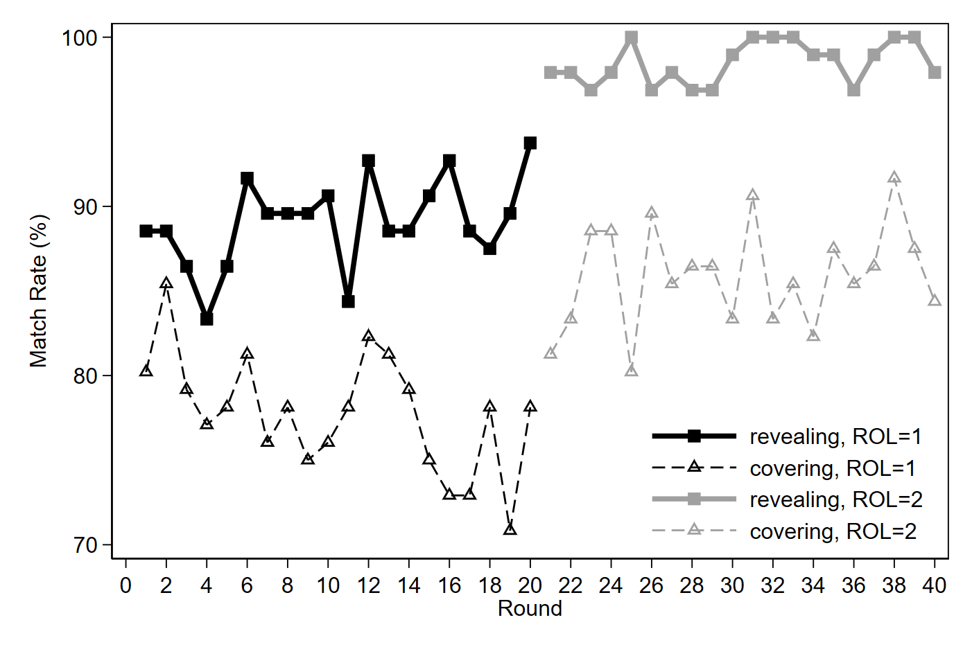
Figure 2: Match rate over round

Neighborhood School Report Rate and Bias

The revealing policy is expected to assist students in making more rational decisions and thereby reduce their propensity to play safe by frequently reporting neighborhood schools. Table 1 presents the neighborhood school report rate under each condition, focusing on students who have neighborhood schools. The table also presents a breakdown of this statistic by each of the four lottery categories. For instance, lottery (1, 4) refers to the four students whose lottery numbers are 1, 2, 3, and 4.

Consistent with our hypothesis, Panel A indicates that the revealing policy results in a significantly lower neighborhood school report rate compared to the covering policy regardless of the ROL length. The report rate across all lottery categories predictably varies under the revealing policy; students who have superior lottery numbers (lower number) are much less likely to report their neighborhood schools than those with inferior lottery numbers. Interestingly, when the ROL length is two, students are increasingly likely to report their neighborhood schools in the first rank as their lottery numbers become worse, even though this is a weakly dominated strategy (as these students could have weakly increased their chances of being admitted to a better school by ranking their neighborhood schools second). By contrast, under the covering policy, as students are not informed of their lottery numbers prior to making decisions, their report rates do not vary much across lottery categories. It is important to note when the ROL length is two, students rarely report their neighborhood schools in the first rank, which constitutes a rational decision. This finding suggests that the high frequency of reporting neighborhood schools in the first rank among students with inferior lottery numbers under the revealing policy is not due to participants’ mistakes. Rather, it may simply reflect their beliefs that they could at best be admitted to their neighborhood schools, regardless of whether they rank it first or second.

Table 1: Neighborhood school report rate and bias

	revealing	covering	p-value
Panel A: Neighborhood school report rate
ROL=1	55.7%	67.5%	0.004
Lottery (1, 4)	2.1%	65.1%	0.002
Lottery (5, 8)	49.4%	64.7%	0.041
Lottery (9, 12)	80.3%	70.2%	0.039
Lottery (12, 16)	92.5%	69.5%	0.002
ROL=2	72.8% (18.6% + 54.2%)	87.8% (3.9% + 83.9%)	0.004
Lottery (1, 4)	43.7% (0.6% + 43.1%)	89.1% (5.7% + 83.3%)	0.002
Lottery (5, 8)	63.2% (13.6% + 49.6%)	86.0% (3.5% + 82.5%)	0.002
Lottery (9, 12)	93.7% (25.3% + 68.4%)	90.8% (2.3% + 88.5%)	0.407
Lottery (12, 16)	97.9% (40.3% + 57.6%)	85.4% (4.2% + 81.3%)	0.004
Panel B: Neighborhood school bias
ROL=2	59.8% (7.7% + 52.1%)	81.9% (1.0% + 80.8%)	0.004
Lottery (1, 4)	9.3% (0% + 9.3%)	82.4% (1.9% + 80.6%)	0.002
Lottery (5, 8)	46.2% (0% + 46.2%)	80.1% (1.9% + 78.2%)	0.002
Lottery (9, 12)	90.8% (10.8% + 80.0%)	86.7% (0% + 86.7%)	0.407
Lottery (12, 16)	100% (25.0% + 75.0%)	78.1% (0% + 78.2%)	0.002

Notes: Under ROL$=$2, the two percentages in the bracket represent the neighborhood school report rate in the first rank and in the second rank, respectively. In Panel A, we focus on students who have neighborhood schools. In Panel B, we only focus on students whose neighborhood school is either C or D when the ROL length is two.

When a student’s neighborhood school is ranked high in payoffs, reporting that school does not necessarily imply neighborhood school bias. We define neighborhood school bias as the tendency to report neighborhood schools when the payoff rankings of these schools do not fall within the very top (when the ROL length is one) or the top two (when the ROL length is two). Under this definition, when the ROL length is one, the neighborhood school report rate is equivalent to the neighborhood school bias. However, when the ROL length is two, the scenario in which a student possesses a neighborhood school B and submits it in her ROL should not be interpreted as neighborhood school bias. Therefore, in Panel B, we only focus on students whose neighborhood schools are either C or D. Despite some level difference, we again find that the revealing policy results in a significantly lower neighborhood school bias compared to the covering policy, with other patterns qualitatively similar to those observed in Panel A.

Segregation

The revealing policy is expected to reduce not only the neighborhood school bias in students’ ROL submissions but also the segregation level in the final admission outcome, measured as the proportion of students assigned to their neighborhood schools. Table 2 in Online Appendix Appendix: Additional Tables indicates that the revealing policy results in a significantly lower segregation level compared to the covering policy, but this effect is significant only when the ROL length is one. When the ROL length is two, although the effect aligns with expectations, the revealing policy exhibits a weaker and statistically insignificant effect on the segregation level. This is primarily driven by the luckiest students who could still be admitted to schools that are better than their neighborhood schools when they have more than one school to report. Thus, their neighborhood school bias has a much weaker impact on their final admission outcomes.

Table 2: Segregation (the proportion of subjects assigned to their neighborhood schools, only for those who have a neighborhood school)

	revealing	covering	p-value
ROL=1	55.7%	67.5%	0.004
Lottery (1, 4)	2.1%	65.1%	0.004
Lottery (5, 8)	49.4%	64.7%	0.035
Lottery (9, 12)	80.3%	70.2%	0.027
Lottery (12, 16)	92.5%	69.5%	0.004
ROL=2	51.7%	52.8%	1.000
Lottery (1, 4)	0.6%	5.7%	0.060
Lottery (5, 8)	41.7%	43.4%	0.868
Lottery (9, 12)	78.2%	85.1%	0.014
Lottery (12, 16)	97.2%	85.4%	0.004

Notes: To examine the segregation rate, we only focus on students who have neighborhood schools. The p-values are produced by the Wilcoxon rank-sum test which compares revealing and covering treatments using each session as an independent observation.

Efficiency

Table 3 reports the efficiency, measured by the student’s average payoff, under each condition. Consistent with our hypothesis, the revealing policy results in significantly greater overall efficiency than the covering policy, irrespective of the ROL length. However, the benefits of the revealing policy are not uniformly distributed among students. While students with the best or worst lottery numbers tend to benefit from this policy, students with intermediate lottery numbers tend to suffer. The issue of unevenly distributed benefits is pronounced when the ROL length is one, but it is largely mitigated when the ROL length is two. Intuitively, when the possibility of mismatch is high (i.e., when the ROL length is short), prior knowledge of lottery numbers assists the most fortunate students in gaining admission to better schools while helping the least fortunate students avoid being left unmatched. However, this dynamic tends to disadvantage students in the middle, making them less likely to gain admission to top schools.

Table 3: Efficiency (mean payoff)

	revealing	covering	p-value
ROL=1	54.6	51.8	0.007
Lottery (1, 4)	87.3	68.0	0.004
Lottery (5, 8)	54.5	64.2	0.004
Lottery (9, 12)	42.6	46.8	0.016
Lottery (12, 16)	33.9	28.1	0.004
ROL=2	59.4	56.0	0.004
Lottery (1, 4)	89.5	84.5	0.004
Lottery (5, 8)	64.9	66.2	0.200
Lottery (9, 12)	47.6	44.1	0.004
Lottery (12, 16)	35.7	29.1	0.004

Notes: The p-values are produced by the Wilcoxon rank-sum test which compares revealing and covering treatments using each session as an independent observation.

ROL Submission Strategies

Following our review of the aggregate-level results, we turn to individual ROL strategies. Table 4 presents the frequency of each possible strategy under each condition. Under the revealing policy, we also calculate the frequency for each lottery category separately. When the ROL length is one, students tend to report better schools more frequently under the covering policy; in contrast, under the revealing policy, the frequency of reporting each school is relatively uniform. The reason is that students make more informed decisions under the revealing policy by primarily reporting schools where they have a realistic chance of admission: students whose lottery numbers range from 1 to 4 are most likely to report school A; students whose lottery numbers range from 5 to 8 are most likely to report school B; and so on. Similarly, when the ROL length is two, under the covering policy, students tend to report a pair of schools that more frequently include at least one top school (such as A-B and A-C) than two bottom schools (such as C-D); conversely, under the revealing policy, the reported pairs of schools are evenly distributed between top and bottom schools (such as A-B, B-C and C-D). Further, students tend to report schools to which they have realistic chances of admission based on their lottery numbers: students whose lottery numbers range from 1 to 4 are most likely to report the school pair A-B; students whose lottery numbers range from 5 to 8 are most likely to report the school pair B-C; students whose lottery numbers range from 9 to 16 are most likely to report the school pair C-D.

Table 4: Proportion of each possible submission strategy (%)

Strategy revealing covering Rank 1 Rank 2 All Lottery (1, 4) Lottery (5, 8) Lottery (9, 12) Lottery (13, 16) All ROL=1 A 25.42 90.63 7.29 1.67 2.08 38.85 B 25.52 7.50 64.17 16.67 13.75 29.11 C 27.45 1.46 25.83 61.67 20.83 21.46 D 21.61 0.42 2.71 20.00 63.33 10.57 ROL=2 A B 32.29 94.79 26.25 5.42 2.71 30.63 A C 1.61 1.67 1.25 2.92 0.63 29.43 A D 0.89 1.04 0 0.63 1.88 12.81 B A 0.78 0.83 1.25 0.42 0.63 1.56 B C 28.85 1.25 66.46 38.96 8.75 14.90 B D 2.81 0 2.50 2.92 5.83 7.45 C A 0.05 0 0 0.21 0 0.10 C B 0.52 0 0.21 1.67 0.21 0.05 C D 29.74 0.42 2.08 46.25 70.21 2.97 D A 0.21 0 0 0 0.83 0.05 D B 0 0 0 0 0 0 D C 2.24 0 0 0.63 8.33 0.05

4 Conclusion

This paper advocates for a “revealing” policy regarding lottery outcomes in school admission systems, contrasting it with the existing “covering” policy. Our analysis underscores the advantages of revealing lotteries prior to preference submission for students facing priority ties. The theoretic analyses show that the revealing policy enhances the decision-making process, allowing students to coordinate their choices more effectively, thereby improving matching outcomes and increasing overall welfare. Further, our complementary lab experiment demonstrates that revealing lotteries leads to higher match rates, reduced neighborhood school bias, minimized segregation, and better alignment of reported preferences with attainable options.

The recent adoption of the revealing policy by NYC indicates a progressive shift towards more transparent and equitable admission processes. Future research should explore the long-term implications of such policy changes, particularly as more data becomes available to assess their impact on school choice dynamics. By providing students with vital information, the revealing policy not only fosters fairness but also promotes informed decision-making, ultimately contributing to more efficient school allocation. This study highlights the essential role of transparency in shaping effective admission mechanisms in educational settings.

Appendix: Additional Tables

Table A1: Proportion of each possible submission strategy (%) for students having neighborhood school B

Strategy revealing covering Rank 1 Rank 2 All Lottery (1, 4) Lottery (5, 8) Lottery (9, 12) Lottery (13, 16) All ROL=1 A 26.25 95.00 6.67 1.67 1.67 10.83 B 72.50 5.00 93.33 96.67 95.00 87.92 C 0.42 0 0 1.67 0 0.83 D 0.83 0 0 0 3.33 0.42 ROL=2 A B 58.33 98.48 56.94 42.59 22.92 90.00 A C 0 0 0 0 0 0 A D 0 0 0 0 0 0 B A 4.17 1.52 5.56 3.70 6.25 6.67 B C 30.00 0 37.50 53.70 33.33 2.50 B D 6.25 0 0 0 31.25 0.42 C A 0 0 0 0 0 0 C B 0 0 0 0 0 0 C D 1.25 0 0 0 6.25 0.42 D A 0 0 0 0 0 0 D B 0 0 0 0 0 0 D C 0 0 0 0 0 0

Table A2: Proportion of each possible submission strategy (%) for students having neighborhood school C

Strategy revealing covering Rank 1 Rank 2 All Lottery (1, 4) Lottery (5, 8) Lottery (9, 12) Lottery (13, 16) All ROL=1 A 22.08 91.67 12.96 0 3.70 15.83 B 15.00 8.33 51.85 4.76 0 12.92 C 61.67 0 35.19 94.05 92.59 71.25 D 1.25 0 0 1.19 3.70 0 ROL=2 A B 24.17 87.04 15.28 0 0 7.50 A C 7.50 9.26 8.33 7.58 4.17 73.75 A D 0 0 0 0 0 0 B A 0 0 0 0 0 0.42 B C 53.33 3.70 76.39 72.73 47.92 15.83 B D 0 0 0 0 0 0.83 C A 0 0 0 0 0 0.83 C B 1.67 0 0 4.55 2.08 0 C D 13.33 0 0 15.15 45.83 0.83 D A 0 0 0 0 0 0 D B 0 0 0 0 0 0 D C 0 0 0 0 0 0

Table A3: Proportion of each possible submission strategy (%) for students having neighborhood school D

Strategy revealing covering Rank 1 Rank 2 All Lottery (1, 4) Lottery (5, 8) Lottery (9, 12) Lottery (13, 16) All ROL=1 A 35.00 96.43 7.14 0 0 22.92 B 14.58 2.38 69.05 0 6.67 19.17 C 17.50 0 19.05 59.26 3.33 14.58 D 32.92 1.19 4.76 40.74 90.00 43.33 ROL=2 A B 28.33 90.74 21.43 1.85 0 13.75 A C 0 0 0 0 0 8.33 A D 1.67 5.56 0 0 2.08 47.92 B A 0 0 0 0 0 1.42 B C 27.50 3.70 65.48 16.67 0 5.00 B D 7.50 0 10.71 9.26 8.33 20.83 C A 0.42 0 0 1.85 0 0 C B 0 0 0 0 0 0 C D 34.17 0 2.38 70.37 87.50 3.33 D A 0 0 0 0 0 0.42 D B 0 0 0 0 0 0 D C 0.42 0 0 0 2.08 0

Table A4: Proportion of each possible submission strategy (%) for non-neighborhood students

Strategy revealing covering Rank 1 Rank 2 All Lottery (1, 4) Lottery (5, 8) Lottery (9, 12) Lottery (13, 16) All ROL=1 A 24.00 87.85 6.48 2.48 2.29 52.25 B 20.42 9.38 60.19 6.38 1.63 22.58 C 28.00 2.43 29.94 65.25 15.69 17.00 D 27.58 0.35 3.40 25.89 80.39 8.17 ROL=2 A B 29.50 96.08 22.22 0.65 0.60 26.75 A C 1.08 0.98 0 2.94 0.30 30.67 A D 1.08 0.65 0 0.98 2.38 10.92 B A 0.42 0.98 0.79 0 0 1.00 B C 24.00 0.65 72.22 33.01 0.89 19.17 B D 1.75 0 1.19 2.94 2.68 7.50 C A 0 0 0 0 0 0 C B 0.50 0 0.40 1.63 0 0.08 C D 37.83 0.65 3.17 56.86 80.36 3.83 D A 0.33 0 0 0 1.19 0 D B 0 0 0 0 0 0 D C 3.50 0 0 0.98 11.61 0.08

Online Appendix: Experimental Instructions

The following instructions are translated from the original instructions in Chinese. The texts which differ between the revealing and covering treatments are highlighted in both italicized and bold face.

General Instructions

You are participating in a decision-making experiment. All participants receive the same experimental instructions, so please read them carefully. During the experiment, no communication is allowed between participants, so please put your phone on silent mode. If you have any questions, feel free to raise your hand, and the experiment staff will come to assist you. You have earned 15 RMB for showing up on time. You can earn additional experimental rewards based on the decisions you make during the experiment. After the experiment concludes, the total points you earn will be converted into RMB at a rate of 2 points = 1 yuan. The final payment will be paid via bank transfer within 2-3 working days. The decisions made by participants in the experiment are completely anonymous, meaning your name will be strictly confidential in the study, and other participants will not know the total experimental rewards you have received today.

In today’s experiment, we will simulate the process of students’ admission to colleges. You and other participants will play the roles of students, and each of you will submit a preference list of schools to the admission system. The system will then assign an admission result to each student. Below are the descriptions of the experimental steps, payoff rules, and admission rules.

Experimental Steps:

• Before the experiment starts, you will be randomly assigned to a 16-person group along with other participants, and each person in the group will play the role of a student. Throughout the experiment, the group members will remain the same. Each group will face four different schools, labeled as A, B, C, and D. Each school has four admission slots, and each slot can admit one student. The admissions for the four schools will be simulated by the computer.

• The experiment consists of 2 modules, each with 20 rounds of decisions.

• In each round of the experiment, you will see the following payoff table, which shows the rewards you can get when being admitted to each school, representing your preferences for different schools. Your payoff depends on the school that admits you. For example, if your payoff table is as follows,

  Admitted School	A	B	C	D	Not Admitted
  Payoff (Points)	95	67	55	26	0

  Then:

  • If school A admits you in a certain round, your payoff for that round will be 95 points.

  • If school B admits you in a certain round, your payoff for that round will be 67 points.

  • … (If any other school admits you, your payoff for that round will be according to the respective school.)

  • If no school admits you in a certain round, your payoff for that round will be 0 points.

• In each round of the experiment, the payoff table for each student is randomly generated by the computer based on the following rules: The payoff for school A is randomly drawn from integers between 81 and 100, the payoff for school B is randomly drawn from integers between 61 and 80, the payoff for school C is randomly drawn from integers between 41 and 60, and the payoff for school D is randomly drawn from integers between 21 and 40. Thus, in each round, the payoff tables for different students are likely to be different. In other words, the payoff from each school may vary for different students.

• In each round, each student needs to submit a preference list of schools. In different modules, you will have the option to submit 1 or 2 schools out of the four schools A, B, C, or D in your preference list. When having the option to submit 2 schools, the two choices cannot be the same school.

• In each round, each student will be randomly assigned an ID within the group. In different rounds, each student’s ID will be regenerated. Based on the student’s ID, some students within the group will be viewed as residing in certain school districts. Specifically:

  • Students with ID 1 or 2 reside in the district of school B.

  • Students with ID 3 or 4 reside in the district of school C.

  • Students with ID 5 or 6 reside in the district of school D.

  • Students with ID 7-16 do not reside in the district of any school.

  • Note: There are 2 students residing in the district of each of schools B, C, and D, while school A does not belong to the district of any student.
    

Admission Rules:

• During the admission process, each school sorts the students based on the “within-district first, outside-district later” rule, and then makes the admissions. Specifically, each school divides all students into two categories:

  • High Priority: Students residing in the school district.

  • Low Priority: Students residing outside the school district.

  Note: Since no student resides in the district of school A, all students are considered to be in the low priority category by school A.

  For students in the same priority category, the computer will randomly draw numbers (lottery) to further sort them.

• Lottery: The students will be assigned random numbers from 1 to 16, and then each school will sort the students in the same priority category based on these lottery numbers, with smaller numbers meaning being ranked higher. [revealing only: In each round, the computer draws the lottery before the students submit their preference lists, and each student is informed of their lottery number before submitting their preference lists.] [covering only: In each round, students first submit their preference lists, and then the computer draws the lottery. Therefore, each student will not know their lottery number before submitting their preference lists.]

  Note: The lottery number is independent of the student’s ID. In different rounds of the experiment, each student’s ID and lottery number will be regenerated.

• Admission Mechanism: [revealing only: In each round, after all students in the group have been informed of their lottery numbers and have submitted their preference lists, the computer will follow these steps to make the admissions:] [covering only: In each round, after all students in each group have submitted their preference lists, the computer draws the lottery, and the admission process proceeds as follows:]

  • Step 1: Send each student’s application to their first-ranked school. After receiving the applications, each school will sort all applicants based on the district and lottery rules mentioned above. Since each school can admit a maximum of 4 students, if a school receives more than 4 applicants, it will temporarily reserve the top 4 applicants according to its sorting and reject the rest.

  • Step 2: (When the option to submit a second-ranked school is available,) send the students rejected by their first-ranked school to their second-ranked school. Upon receiving the new applications, each school will sort the new applicants along with the previously reserved applicants. If a school receives more than 4 applicants, it will temporarily reserve the top 4 applicants according to its sorting and reject the rest. (Note: The students rejected in Step 2 can be either new applicants or previously reserved applicants.)

  • Step 3: (When the option to submit a second-ranked school is available,) if there are students among the rejected students from the previous step who have not been sent to their second-ranked school yet (i.e., they were only rejected by their first-ranked school), send their applications to their second-ranked school. Again, each school will sort the new applicants along with the previously reserved applicants. If a school receives more than 4 applicants, it will temporarily reserve the top 4 applicants according to its sorting and reject the rest. (Note: The students rejected in Step 3 can be either new applicants or previously reserved applicants.)

  • If necessary, repeat Step 3 until each student is either reserved by a certain school or rejected by all schools. At this point, the students retained by each school are the officially admitted students, while the students rejected by all schools are not admitted.

An Example:

Let’s use an example to further explain the admission rules. For simplicity, we will consider 3 schools and 6 students.

Students and Schools: The IDs of the 6 students are 1, 2, 3, 4, 5, and 6; there are 3 schools: A, B, and C.

Admission Slots: Each school has 2 admission slots.

Payoff Rankings: Each student has the same ranking of schools and payoffs: $A>B>C$

District Schools: Student 1 resides in the district of school A, student 2 resides in the district of school B, student 3 resides in the district of school C. Other students do not reside in the district of any school.

Priorities: According to the district rules, each school’s priority ranking for all students is as follows (the numbers in the table represent student IDs):

School	High Priority (District)	Low Priority (Non-District)
A	1	2, 3, 4, 5, 6
B	2	1, 3, 4, 5, 6
C	3	1, 2, 4, 5, 6

Lottery Results: Let’s assume the lottery results are as shown below (lower numbers indicate higher rankings):

Lottery Number	1	2	3	4	5	6
Student ID	3	6	4	5	2	1

Final Sorting After Lottery: Based on the district rules and lottery results, each school’s sorting of students during admissions is as follows:

School	Sort 1 (District)	Sort 2	Sort 3	Sort 4	Sort 5	Sort 6
A	1	3	6	4	5	2
B	2	3	6	4	5	1
C	3	6	4	5	2	1

Preference List: Let’s assume the students submit the following preference lists:

	Student 1	Student 2	Student 3	Student 4	Student 5	Student 6
First-ranked School	A	A	A	A	B	A
Second-ranked School	B	B	C	B	C	B

Admissions Process:

Step 1: Send each student’s application to their first-ranked school.

- School A reserves students 1 and 3, rejects students 2, 4, and 6.

- School B reserves student 5. School C receives no applications.

Application		School		Reserved	Rejected
1,2,3,4,6	$\rightarrow$	A	$\rightarrow$	1,3	2,4,6
5	$\rightarrow$	B	$\rightarrow$	5
	$\rightarrow$	C	$\rightarrow$

Step 2: Students rejected in the previous step apply to their second-ranked school. Therefore, students 2, 4, and 6 apply to School B.

- School B receives applications from students 2, 4, and 6. After sorting, it reserves students 2 and 6, and rejects students 4 and 5.

Previously Reserved	New Applications		School		Reserved	Rejected
1,3		$\rightarrow$	A	$\rightarrow$	1,3
5	2,4,6	$\rightarrow$	B	$\rightarrow$	2,6	4,5
		$\rightarrow$	C	$\rightarrow$

Step 3: Students who are rejected in the previous step and have not yet applied to their second-ranked school, apply to their second-ranked school. Since student 4 has already been rejected by their second-ranked school, they can no longer apply to any school. Student 5 applies to School C as their second choice.

- School C reserves student 5.

Previously Reserved	New Applications		School		Reserved	Rejected
1,3		$\rightarrow$	A	$\rightarrow$	1,3
2,6		$\rightarrow$	B	$\rightarrow$	2,6
	5	$\rightarrow$	C	$\rightarrow$	5

The final admission results are as follows:

Student ID	1	2	3	4	5	6
Admitted School	A	B	A	Not Admitted	C	B

Payoff Rules:

• At the end of each round of the experiment, each student will be informed of whether they have been admitted, the school they have been admitted to, and their payoff. Note that each student’s admission result in each round is independent of their admission results in previous rounds.

• After all 40 rounds of the experiment, we will randomly select one round of admission results from each module as your payoff for that module. Your total payoff will be the sum of the payoffs from these two modules. Additionally, you will receive a participation fee of 15 RMB. Finally, you can also earn additional income from the post-experiment questionnaire.

References

- (1)
- Abdulkadiroğlu, Pathak and Roth (2009) Abdulkadiroğlu, Atila, Parag A Pathak, and Alvin E Roth. 2009. “Strategy-proofness versus efficiency in matching with indifferences: Redesigning the NYC high school match.” American Economic Review, 99(5): 1954–78.
- Abdulkadiroglu, Che and Yasuda (2011) Abdulkadiroglu, Atila, Yeon-Koo Che, and Yosuke Yasuda. 2011. “Resolving Conflicting Preferences in School Choice: The" Boston Mechanism" Reconsidered.” American Economic Review, 101(1): 399–410.
- Akbarpour et al. (2022) Akbarpour, Mohammad, Adam Kapor, Christopher Neilson, Winnie Van Dijk, and Seth Zimmerman. 2022. “Centralized school choice with unequal outside options.” Journal of Public Economics, 210: 104644.
- Arnosti (2023) Arnosti, Nick. 2023. “Lottery design for school choice.” Management Science, 69(1): 244–259.
- Ashlagi and Nikzad (2020) Ashlagi, Itai, and Afshin Nikzad. 2020. “What matters in school choice tie-breaking? How competition guides design.” Journal of Economic Theory, 190: 105120.
- Azevedo and Leshno (2016) Azevedo, Eduardo M, and Jacob D Leshno. 2016. “A supply and demand framework for two-sided matching markets.” Journal of Political Economy, 124(5): 1235–1268.
- Calsamiglia, Haeringer and Klijn (2010) Calsamiglia, Caterina, Guillaume Haeringer, and Flip Klijn. 2010. “Constrained school choice: An experimental study.” The American Economic Review, 1860–1874.
- Featherstone and Niederle (2016) Featherstone, Clayton R, and Muriel Niederle. 2016. “Boston versus deferred acceptance in an interim setting: An experimental investigation.” Games and Economic Behavior, 100: 353–375.
- Fischbacher (2007) Fischbacher, Urs. 2007. “z-Tree: Zurich toolbox for ready-made economic experiments.” Experimental Economics, 10(2): 171–178.
- Marian (2023) Marian, Amelie. 2023. “Algorithmic Transparency and Accountability through Crowdsourcing: A Study of the NYC School Admission Lottery.” 434–443.
- Pathak and Sethuraman (2011) Pathak, Parag A, and Jay Sethuraman. 2011. “Lotteries in student assignment: An equivalence result.” Theoretical Economics, 6(1): 1–17.
- Roth and Sotomayor (1992) Roth, Alvin E, and Marilda A Oliveira Sotomayor. 1992. Two-sided matching: A study in game-theoretic modeling and analysis. Cambridge University Press.