Beam Domain Channel Estimation for Spatial Non-Stationary Massive MIMO Systems

Abstract

In massive multiple-input multiple-output (MIMO) systems, the channel estimation scheme is subject to the spatial non-stationarity and inevitably power leakage in the beam domain. In this paper, a beam domain channel estimation scheme is investigated for spatial non-stationary (SNS) massive MIMO systems considering power leakage. Specifically, a realistic massive MIMO beam domain channel model (BDCM) is introduced to capture the spatial non-stationarity considering power leakage by introducing the illustration of visibility region (VR). Then, a beam domain structure-based sparsity adaptive matching pursuit (BDS-SAMP) scheme is proposed based on the cross-block sparse structure and power ratio threshold of beam domain channel. Finally, the simulation results validate the accuracy of proposed BDS-SAMP scheme with low pilot overhead and reasonable complexity by comparing with conventional schemes.

I Introduction

In recent years, massive MIMO has attracted wide attention due to the improvement in efficiency of spectrum and energy [1, 2]. However, the computational complexity of channel modeling and the overhead of channel estimation are challenging task because of the large number of antennas [4, 3]. The BDCM, transferring the channel model from array domain into the beam domain, can reduce the computational complexity and play a critical role in the design and performance evaluation [5]. In order to fully maintain the beamforming gains of massive MIMO beam domain channels, it is essential to obtain accurate knowledge of channel state information (CSI).

Massive MIMO beam domain channels display sparsity with a small number of channel elements containing most of the energy [6]. Numerous channel estimation algorithms based on the compressed sensing (CS) [7] including convex optimization algorithms [8], Bayesian algorithms [9], and greedy algorithms [10] have been employed for massive MIMO systems by leveraging the inherent sparsity of channels. Due to the advantages in terms of implementation simplicity and computational efficiency, greedy algorithms such as orthogonal matching pursuit (OMP), sparse adaptive matching pursuit (SAMP) [11], and block-based OMP (BOMP) [12] have been used for massive MIMO channel estimation. Nevertheless, the above-mentioned algorithms considered massive MIMO channels to be spatial stationary (SS) with identical sparse structure. In practice, massive MIMO channels are SNS with some scatterers visible only to a portion of the antenna array [13], resulting in varied sparse structure over array.

In [14] and [15], the authors modified the standardized 3GPP channel model to capture the spatial non-stationarity by using birth-death process, and then performed array domain channel estimation for SNS massive MIMO systems. However, they ignored the inevitably impact of channel power leakage on the sparsity and estimation performance since massive MIMO channels are not ideally sparse in practice. In [16] and [17], the channel estimation schemes based on support detection (SD) [18], e.g., adaptive SD (ASD) and successive SD, were proposed by making full use of adaptive updated or successive rectangle support structure of beam domain channel considering power leakage. However, these schemes were based on SS massive MIMO channels assumption, which will further underestimate the power leakage of beam domain channel and cause inaccurate results of channel estimation.

To the best of our knowledge, beam domain channel estimation for SNS massive MIMO systems is still lacking in the literature. To fill this research gap, a BDS-SAMP channel estimation scheme is proposed for SNS massive MIMO systems considering sparse structure and power leakage of beam domain channel. The main contributions and novelties of this paper are summarized as below.

• A realistic massive MIMO BDCM is introduced to capture spatial non-stationarity by introducing the VR of different clusters. Furthermore, the beam sparse structure and power leakage effect are demonstrated.

• A BDS-SAMP channel estimation scheme for SNS massive MIMO systems is proposed, in which the beam support set is iteratively obtained based on the cross-block sparse structure and power ratio threshold of beam domain channel.

• Simulation results verify the accuracy and robustness of proposed BDS-SAMP scheme by comparing with the traditional channel estimation schemes.

The remainder of this paper is organized as follows. Section II introduces the system model including SNS massive MIMO BDCM and problem formulation. Based on it, Section III analyzes the power leakage effect. In section IV, a BDS-SAMP channel estimation scheme for SNS massive MIMO systems is proposed. Section V presents the simulation results and demonstrates the predominant performance of the proposed scheme. Finally, conclusions are drawn in Section VI.

II System Model

Channel estimation schemes are highly dependent on channel models. The realistic channel model is the basis for system performance evaluation and accurate channel estimation. In this section, a realistic SNS massive MIMO BDCM is introduced by introducing the illustration of VR. Based on it, the beam domain channel estimation problem is formulated.

II-A SNS Massive MIMO BDCM

We consider a downlink massive MIMO system as shown in Fig. 1, where the base station (BS) employs a large uniform planar array (UPA) with ${P}$ antennas and serves $U$ single-antenna users. Here, $P$ consists of ${P_{v}}$ antenna elements in vertical dimension multiplied by ${P_{h}}$ antenna elements in horizontal dimension.

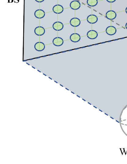
Figure 1: System structure diagram for massive MIMO systems.

We classify all clusters in massive MIMO systems into wholly visible (WV) clusters and partially visible (PV) clusters [5]. Each cluster has a corresponding VR, the VR of WV clusters is the entire array, while that of PV clusters is the partial array. The ratio of PV clusters to total clusters is $\rho$. We start with the geometry-based stochastic channel model (GBSM) for massive MIMO to obtain array domain channel transfer function (CTF). The CTF matrix for the $u$th $(u=1,2,...,U)$ user can be written as

$${\mathbf{H}_{u}}={{\mathbf{H}}_{u}^{{\text{WV}}}}+{{\mathbf{H}}_{u}^{{\text{PV}}}}$$ (1)

where ${\mathbf{H}}_{u}^{{\text{WV}}}$ and ${\mathbf{H}}_{u}^{{\text{PV}}}$ are CTF matrices of WV and PV multipath components (MPCs), which can be formulated as

$${\mathbf{H}}_{u}^{{\text{WV}}}=\sum\limits_{n\in{{\mathbf{N}}_{1}}}{\sum\limits_{m=1}^{{M_{n}}}{{\beta_{n,m}}{e^{{\rm j}\psi_{n,m}}}}}{{{\mathbf{U}}\left({\theta_{n,m}^{az},\theta_{n,m}^{el}}\right)}}$$ (2)

$${{\mathbf{H}}_{u}^{{\text{PV}}}}=\sum\limits_{n\in{{\mathbf{N}}_{2}}}{\sum\limits_{m=1}^{{M_{n}}}{{\beta_{n,m}}{e^{{\rm j}\psi_{n,m}}}}}{{\mathbf{\hat{U}}}\left({\theta_{n,m}^{az},\theta_{n,m}^{el}}\right)}$$ (3)

with

$$\psi_{n,m}={-2\pi f{\tau_{n,m}}+{\varphi_{n,m}}}.$$ (4)

Here, $f$ indicates the carrier frequency, $M_{n}$ stands for the paths number of the $n$th cluster, ${\bf{N}}_{1/2}$ are the sets of the WV/PV clusters, $\varphi_{n,m}$, $\tau_{n,m}$ and ${\beta_{n,m}}$ denote the random initial phase, delay and coefficient of $m$th path in the $n$th cluster, respectively. To avoid redundancy, abbreviate all variables whose subscript is (${n,m}$) as that of $m_{n}$th path in the following part. The UPA steering matrix for WV clusters is defined as ${\bf{U}}\left({\theta_{n,m}^{az},\theta_{n,m}^{el}}\right)={\left[{{\mathbf{b}}\left({\theta_{n,m}^{el}}\right)\otimes{\mathbf{a}}\left({\theta_{n,m}^{az}}\right)}\right]}^{\text{T}}$, where ${\mathbf{a}}\left({\theta_{n,m}^{az}}\right)={\left[{1,{e^{{\rm j}2\pi\theta_{n,m}^{az}}},\cdots,{e^{{\rm j}2\pi\left({{P_{h}}-1}\right)\theta_{n,m}^{az}}}}\right]^{\text{T}}}$ and ${\mathbf{b}}\left({\theta_{n,m}^{el}}\right)={\left[{1,{e^{{\rm j}2\pi\theta_{n,m}^{el}}},\cdots,{e^{{\rm j}2\pi\left({{P_{v}}-1}\right)\theta_{n,m}^{el}}}}\right]^{\text{T}}}$ with $\theta_{n,m}^{az}$ and $\theta_{n,m}^{el}$ standing for the spatial frequencies in azimuth and elevation directions associated with the $m_{n}$th path. Without loss of generality, we usually set adjacent antennas spacing as half wavelength, thus $\theta_{n,m}^{az/el}\in\left[{-0.5,0.5}\right]$. Furthermore, the steering matrix for PV clusters can be obtained via ${\bf{\hat{U}}}\left({\theta_{n,m}^{az},\theta_{n,m}^{el}}\right)={\bf{U}}\left({\theta_{n,m}^{az},\theta_{n,m}^{el}}\right)\odot{{\mathbf{\xi}}_{n,m}}$. The VR of $m_{n}$th path is defined by the matrix $\mathbf{\xi}_{n,m}$ consisting only of 0 and 1, which indicates the visibility of cluster to antenna array.

Figure 2: Flowchart of generating the SNS BDCM.

The BDCMs can be obtained by unitary transformation of GBSMs [19]. For clarity, the brief flowchart of generating the SNS BDCM is shown in Fig. 2. The array domain CTF $\textbf{H}_{u}$ can be converted to the beam domain CTF $\textbf{H}{{}_{\text{B},u}}$ by two-dimensional DFT processing as follows

$${{\bf{H}}_{\text{B},u}}={\bf{F}}_{{}^{el}}^{*}{\bf{H}}_{u}{\bf{F}}_{{}^{az}}^{\text{T}}$$ (5)

with

$${\bf{F}}_{{}^{el}}=\frac{1}{{\sqrt{{P_{v}}}}}\left[{\mathbf{b}}\left({\tilde{\theta}_{i}^{el}}\right)\right]_{i=1,2,...,{P_{v}}}^{\text{T}}$$ (6)

$${\bf{F}}_{{}^{az}}=\frac{1}{{\sqrt{{P_{h}}}}}\left[{\mathbf{a}}\left({\tilde{\theta}_{j}^{az}}\right)\right]_{j=1,2,...,{P_{h}}}^{\text{T}}$$ (7)

where $\tilde{\theta}_{i}^{el}$ and $\tilde{\theta}_{j}^{az}$ are the predetermined elevation and azimuth spatial frequencies of beam domain, and F_el and F_az represent the elevation and azimuth beamforming matrices, respectively. By substituting (1) into (5), the ${\mathbf{H}_{\text{B},u}}$ can be rewritten as

$${\mathbf{H}_{\text{B},u}}={{\mathbf{H}}_{\text{B},u}^{{\text{WV}}}}+{{\mathbf{H}}_{\text{B},u}^{{\text{PV}}}}.$$ (8)

where ${{\mathbf{H}}_{\text{B},u}^{{\text{WV}}}}$ and ${{\mathbf{H}}_{\text{B},u}^{{\text{PV}}}}$ are beam domain CTF matrices of WV and PV MPCs.

II-B Problem Formulation

This paper adopts the orthogonal pilot transmission strategy and mainly focus on the downlink. Suppose BS repeatedly sends pilot sequences with the length of $U$ to different users for $Q$ times, and the channel experiences the same fading during $K=U\times Q$ time slots. The pilot sequence sent from BS to the users forms the pilot matrix ${\bf{X}}\in{\mathbb{C}^{U\times U}}$. When transmitting the $q$th $(q=1,2,...,Q)$ pilot sequence, the BS employs an analog precoder ${{\bf{F}}_{q}}\in{\mathbb{C}^{U\times P}}$, and the received signals by the $u$th user can be presented by

$${{\bf{r}}_{u,q}}={\bf{X}}{{\bf{F}}_{q}}{{\bf{h}}_{u}}+{{\bf{n}}_{u,q}}$$ (9)

where ${{\bf{h}}_{u}}\in{\mathbb{C}^{P\times 1}}$ is the channel vector rearranged by ${{\bf{H}}_{u}}$, ${{\bf{n}}_{u,q}}\in{\mathbb{C}^{U\times 1}}$ is the additive white Gaussian noise vector satisfying ${{\bf{n}}_{u,q}}\sim{\cal C}{\cal N}(0,{\sigma^{2}}{{\bf{I}}_{U}})$ with $\sigma^{2}$ standing for the noise power. Due to the orthogonality of ${\bf{X}}$, i.e., ${\bf{X}}{{\bf{X}}^{\rm{H}}}={{\rm I}_{U}}$, we can obtain

$${{\bf{y}}_{u,q}}={{\bf{X}}^{\rm{H}}}{{\bf{r}}_{u,q}}={{\bf{F}}_{q}}{{\bf{h}}_{u}}+{{{\bf{\tilde{n}}}}_{u,q}}$$ (10)

where ${{{\bf{\tilde{n}}}}_{u,q}}={{\bf{X}}^{\rm{H}}}{{\bf{n}}_{u,q}}$. Define ${\bf{\tilde{U}}}={{\bf{F}}_{el}}\otimes{{\bf{F}}_{az}}\in{\mathbb{C}^{P\times P}}$, ${{\bf{y}}_{u,q}}$ in (10) can be rewritten as

$${{\bf{y}}_{u,q}}={{\bf{\Phi}}_{q}}{{\bf{h}}_{\text{B},u}}+{{{\bf{\tilde{n}}}}_{u,q}}$$ (11)

where ${{\bf{\Phi}}_{q}}={{\bf{F}}_{q}}{{{\bf{\tilde{U}}}}^{\rm{H}}}$, and ${{\bf{h}}_{\text{B},u}}\in{\mathbb{C}^{P\times 1}}$ is the channel vector rearranged by ${{\bf{H}}_{\text{B},u}}$ satisfying ${{\bf{h}}_{\text{B},u}}={{{\bf{\tilde{U}}}}}{{\bf{h}}_{u}}$ according to (8). After $Q$ times repetitive pilot transmission, the received signal can be written as

$${{\bf{y}}_{u}}={\bf{\Phi}}{{\bf{h}}_{\text{B},u}}+{{{\bf{\tilde{n}}}}_{u}}$$ (12)

where ${{\bf{y}}_{u}}\buildrel\Delta\over{=}{\left[{{\bf{y}}_{u,1}^{\rm{T}},{\bf{y}}_{u,2}^{\rm{T}},...,{\bf{y}}_{u,Q}^{\rm{T}}}\right]^{\rm{T}}}\in{\mathbb{C}^{K\times 1}}$, ${\bf{\Phi}}\buildrel\Delta\over{=}{\left[{{\bf{\Phi}}_{1}^{\rm{T}},{\bf{\Phi}}_{2}^{\rm{T}},...,{\bf{\Phi}}_{Q}^{\rm{T}}}\right]^{\rm{T}}}\in{\mathbb{C}^{K\times P}}$ represents the measurement matrix, and ${{{\bf{\tilde{n}}}}_{u}}\buildrel\Delta\over{=}{\left[{{\bf{\tilde{n}}}{{{}_{u,1}^{\rm{T}}}},{\bf{\tilde{n}}}{{{}_{u,2}^{\rm{T}}}},...,{\bf{\tilde{n}}}{{{}_{u,Q}^{\rm{T}}}}}\right]^{\rm{T}}}\in{\mathbb{C}^{K\times 1}}$. Owing to the sparsity of vector ${\bf{h}}_{\text{B},u}$, (12) can be regarded as sparse signal recovery problem. However, massive MIMO channels are not ideally sparse in practice due to the power leakage, which challenges the channel recovery performance. To better solve the problem of beam domain channel estimation, the power leakage effect is detailed introduced in next section.

III Analysis of Power Leakage

The sparse structure of SNS massive MIMO beam domain channel is visualized in Fig. 3. It is notable that the channel amplitudes are only concentrated within a small part of the beams and the dominant beams form the shape of cross-blocks. However, it is not ideally sparse. The fact that the power of small nonzero amplitudes spreads over other beam directions refers to power leakage. In massive MIMO beam domain channels, power leakage inevitably exists between beams due to the limited beamspace resolution of small VRs and imperfect beam sampling [5].

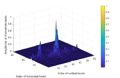
Figure 3: Sparse structure of SNS massive MIMO beam domain channel.

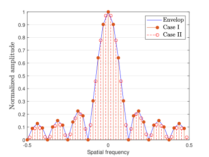
Figure 4: Envelop of ${f_{I_{s}^{h},I_{e}^{h}}}\left({\theta_{0}^{az}-\tilde{\theta}_{j}^{az}}\right)$ ($\theta_{0}^{az}=0,I_{s}^{h}=P_{h}/4,I_{e}^{h}=P_{h}/2-1$).

The beam domain channel representation of the $(i,j)$th beam between the BS and $u$th user can be formulated as

$${{\bf{h}}_{\text{B},u(i,j)}}={{\mathbf{h}}_{\text{B},u(i,j)}^{{\text{WV}}}}+{{\mathbf{h}}_{\text{B},u(i,j)}^{{\text{PV}}}}$$ (13)

where

$$\begin{gathered}{{\mathbf{h}}_{\text{B},u(i,j)}^{{\text{WV}}}}=\frac{1}{{\sqrt{P}}}\sum\limits_{n\in{{\mathbf{N}}_{1}}}{\sum\limits_{m=1}^{{M_{n}}}{{\beta_{n,m}}{e^{{\rm j}\psi_{n,m}}}}}\hfill\\ \times{f_{1,{P_{v}}}}\left({\theta_{n,m}^{el}-\tilde{\theta}_{i}^{el}}\right){f_{1,{P_{h}}}}\left({\theta_{n,m}^{az}-\tilde{\theta}_{j}^{az}}\right)\hfill\\ \end{gathered}$$ (14)

$$\begin{gathered}{{\mathbf{h}}_{\text{B},u(i,j)}^{{\text{PV}}}}=\frac{1}{{\sqrt{P}}}\sum\limits_{n\in{{\mathbf{N}}_{2}}}{\sum\limits_{m=1}^{{M_{n}}}{{\beta_{n,m}}{e^{{\rm j}\psi_{n,m}}}}}\hfill\\ \times{f_{I_{s,nm}^{v},I_{e,nm}^{v}}}\left({\theta_{n,m}^{el}-\tilde{\theta}_{i}^{el}}\right){f_{I_{s,nm}^{h},I_{e,nm}^{h}}}\left({\theta_{n,m}^{az}-\tilde{\theta}_{j}^{az}}\right)\hfill\\ \end{gathered}$$ (15)

with

$${f_{I_{s},I_{e}}}\left(x\right)={e^{j\pi x({I_{s}}+{I_{e}}-2)}}\frac{{\sin\left[{\pi x({I_{e}}-{I_{s}}+1)}\right]}}{{\sin\left[{\pi x}\right]}}$$ (16)

where ${I_{s,nm}^{h/v}}$ and ${I_{e,nm}^{h/v}}$ represent the start and end column/row indices of VR for the $m_{n}$th path, respectively.

Note that ${f_{I_{s},I_{e}}}\left(x\right)$ in (16) is the Dirichlet sinc function. When $\rho=0$, the channel model degenerates to SS resulting in the narrowest beam, which is already taken into account in most beam domain channel estimate schemes. In this case, if the physical direction of the MPCs is perfectly sampled, i.e., $\tilde{\theta}_{i}^{el}\in{{\rm{\Lambda}}_{1}}\buildrel\Delta\over{=}\left\{{i/{P_{v}}-0.5,i=1,2,...,{P_{v}}}\right\}$ and $\tilde{\theta}_{j}^{az}\in{{\rm{\Lambda}}_{2}}\buildrel\Delta\over{=}\left\{{j/{P_{h}}-0.5,j=1,2,...,{P_{h}}}\right\}$, no power leakage will occur. However, in most cases $\tilde{\theta}_{i}^{el}\notin{{\rm{\Lambda}}_{1}}$ or $\tilde{\theta}_{j}^{az}\notin{{\rm{\Lambda}}_{2}}$, thus the WV MPCs result in power leakage, which is manifested by two peaks in the main beam of its envelope [20].

When PV MPCs are considered in massive MIMO systems, the beam widens and the power leakage becomes complicated. Fig. 4 shows the normalized amplitude of ${f_{I_{s}^{h},I_{e}^{h}}}\left({\theta_{0}^{az}-\tilde{\theta}_{j}^{az}}\right)$ for PV MPCs with $\rho=1$ and ${P_{h}}=32$. The envelop of ${f_{I_{s}^{v},I_{e}^{v}}}\left({\theta_{0}^{el}-\tilde{\theta}_{i}^{el}}\right)$ is similar as ${f_{I_{s}^{h},I_{e}^{h}}}\left({\theta_{0}^{az}-\tilde{\theta}_{j}^{az}}\right)$. The horizontal length of VR is 8 continuous antenna elements. It can be readily seen that ${f_{I_{s}^{h},I_{e}^{h}}}\left({\theta_{0}^{az}-\tilde{\theta}_{j}^{az}}\right)$ are uniformly sampled at direction $\tilde{\theta}_{j}^{az}$ and are peaky around $\theta_{0}^{az}$. Due to the partial visibility of MPCs, the power leakage can be observed inevitably under case I, i.e., $\tilde{\theta}_{j}^{az}\in{{\rm{\Lambda}}_{2}}$, which results in minimal power leakage, and case II, i.e., $\tilde{\theta}_{j}^{az}\notin{{\rm{\Lambda}}_{2}}$, which maximizes the power leakage.

IV BDS-SAMP Channel Estimation Scheme

Due to the sparsity and the inevitable power leakage of SNS MIMO beam domain channel, it is necessary to consider the sparse structure and power leakage effect when performing channel estimation. In this section, a BDS-SAMP algorithm for SNS massive MIMO beam domain channel estimation is proposed, in which the beam support set is iteratively obtained based on the cross-block sparse structure and power ratio threshold of beam domain channel. The pseudo-code of the proposed scheme is summarized in Algorithm 1, which can be explained in detail as follows.

Define the residual vector of the $(k-1)$th iteration as ${{\mathbf{r}_{k-1}}}\in{\mathbb{C}^{K\times{1}}}$ and beam correlation between residual vector and $p$th column of measurement matrix ${\bf{\Phi}}_{p}$ as $c_{p}={{\bf{\Phi}}_{p}^{\rm{H}}{\mathbf{r}_{k-1}}}$. The beam with higher $c_{p}$ means it is easier to be selected into the beam support set. Therefore, the column most relevant to residual vector can be obtained by

$${S_{k}}=\text{max}\left\{{\left|c_{p}\right|_{p=1}^{P},s}\right\}$$ (17)

where ${S_{k}}$ is the preliminary beam support set. In order to find out the dominant beam supports quickly, we have to determine the entries on the top, bottom, left, and right of ${S_{k}}$ based on the cross-block of beam domain channel, and denote them as ${{\Upsilon}\in\Omega}$, $\Omega\triangleq\{1,2,\ldots,P\}$. Define the power ratio threshold as $\mu\in\left({0,1}\right]$. Then compute the power ratio of the strongest beam entry ${S_{k}}$ over all the dominant beam supports as

$$\tilde{\mu}={{{{\mathbf{h}}_{\text{B},u[{S_{k}}]}}}\mathord{\left/{\vphantom{{{{\mathbf{h}}_{\text{B},u[{S_{k}}]}}}{\left({{{\mathbf{h}}_{\text{B}(u)[{S_{p}}]}}+\sum\limits_{i\in\Upsilon}{{{\mathbf{H}}_{\text{B}(u)[i]}}}}\right)}}}\right.\kern-1.2pt}{\left({{{\mathbf{h}}_{\text{B},u[{S_{k}}]}}+\sum\limits_{i\in\Upsilon}{{{\mathbf{h}}_{\text{B},u[i]}}}}\right)}}$$ (18)

and refine preliminary beam support set ${S_{k}}$ via

$${S_{k}}={S_{k}}\cup\Upsilon$$ (19)

with $\tilde{\mu}\geqslant\mu$.

Next, we get candidate list ${C_{k}}$ via an union ${C_{k}}={\Omega_{s}}\cup{S_{k}}$ and then obtain final test via

$$F=\text{max}\left\{{\left|{{{\left({{\bf{\Phi}}_{p}^{\rm{H}}{\bf{\Phi}}_{p}}\right)}^{-1}}{\bf{\Phi}}_{p}^{\rm{H}}{\mathbf{y}}_{u}}\right|_{p=1}^{\text{card}({C_{k}})},s}\right\}.$$ (20)

The initial estimation of dominant entries of ${{\mathbf{h}}_{\text{B},u}}$ is

$${{\mathbf{\hat{h}}}}_{\text{B},u}[F]={\left({{\bf{\Phi}}_{F}^{\rm{H}}{\bf{\Phi}}_{F}}\right)^{-1}}{\bf{\Phi}}_{F}^{\rm{H}}{\mathbf{y}_{u}}$$ (21)

which is obtained by essentially least squares (LS) estimation. To get the refined beam support set, the residual vector should be updated via

$${{\mathbf{r}}_{F}}={\mathbf{y}}_{u}-{\bf{\Phi}}_{F}{{\mathbf{\hat{h}}}}_{\text{B},u}[F].$$ (22)

Algorithm 1 Proposed BDS-SAMP Scheme

1:The received signal ${\bf y}_{u}$, measurement matrix ${\bf{\Phi}}$, power ratio threshold $\mu$ and step size $s$ = 1.

2:Estimated beam domain channel for user $u$: ${{\bf{\hat{h}}}_{\text{B},u}}$.

3:Initialization: Initial residual vector ${{\mathbf{r}}_{0}}={\mathbf{y}_{u}}$; Support set ${\Omega_{s}}=\emptyset$; Iteration index $k$ = 1.

4:while $k\leq K$ do

5:  Obtain ${S_{k}}$ via (17);

6:  Obtain $\tilde{\mu}$ via (18);

7:  if $\tilde{\mu}\geqslant\mu$ then

8:   Update ${S_{k}}$ via (19);

9:  end if

10:  Make candidate list via ${C_{k}}={\Omega_{s}}\cup{S_{k}}$;

11:  Obtain final test $F$ via (20);

12:  Obtain LS estimation ${{\mathbf{\hat{h}}}}_{\text{B},u}[F]$ via (21) ;

13:  Compute residual ${{\mathbf{r}}_{F}}$ via (22);

14:  if $\left\|{{{\mathbf{r}}_{F}}}\right\|_{2}^{2}<{\mathbf{r}}$ then

15:   ${\Omega_{s}}=F$;

16:   ${{\mathbf{r}}_{k}}={{\mathbf{r}}_{F}}$;

17:   break;

18:  else if ${{\mathbf{r}}_{F}}\geqslant{{\mathbf{r}}_{k-1}}$ then

19:   $s=s+1$;

20:  else

21:   ${\Omega_{s}}=F$;

22:   ${{\mathbf{r}}_{k}}={{\mathbf{r}}_{F}}$;

23:   $k=k+1$;

24:  end if

25:end while

26:return ${{\mathbf{\hat{h}}}}_{\text{B},u}[{\Omega_{s}}]$ via (24).

Since noise can affect the received signal in different channel states, the stop iteration threshold parameters need to be set differently according to the channel states. The signal-to-noise ratio (SNR) is used to characterize the channel state, and the stop iteration threshold of algorithm under different SNR is set by [15]

$${\mathbf{r}}={{\left\|{\mathbf{y}}_{u}\right\|_{2}^{2}}\mathord{\left/{\vphantom{{\left\|{\mathbf{Y}}\right\|_{2}^{2}}{({{10}^{{\text{SNR}\mathord{\left/{\vphantom{\text{SNR}{10}}}\right.\kern-1.2pt}{10}}}}+1)}}}\right.\kern-1.2pt}{({{10}^{{\text{SNR}\mathord{\left/{\vphantom{\text{SNR}{10}}}\right.\kern-1.2pt}{10}}}}+1)}}.$$ (23)

If the residual vector satisfies $\left\|{{{\mathbf{r}}_{F}}}\right\|_{2}^{2}<{\mathbf{r}}$, then the beam support set and residual vector can be updated. Otherwise, compare the current residual vector ${{\mathbf{r}}_{F}}$ with the residual of the previous iteration ${{\mathbf{r}}_{k-1}}$ to update the support set, residual vector, and number of iterations. Repeat the above steps to get beam support set ${\Omega_{s}}$ until all the pilot information has been used, and finally get the estimated channel via

$${{\mathbf{\hat{h}}}}_{\text{B},u}[{\Omega_{s}}]={\left({{\bf{\Phi}}_{\Omega_{s}}^{\rm{H}}{\bf{\Phi}}_{\Omega_{s}}}\right)^{-1}}{\bf{\Phi}}_{\Omega_{s}}^{\rm{H}}{\mathbf{y}_{u}}.$$ (24)

Note that if the beam support refinement from step 4 to step 7 is deleted, the scheme will be reduced to the SAMP. The calculations of (18) and (19) are performed offline without additional computational complexity. The main complexity of the algorithm focuses on the matrix inverse operations in step 9 and 10, resulting in the computational complexity of ${\rm O}(2K^{\frac{3}{2}})$. In the proposed BDS-SAMP algorithm, the dimension of residual vector ${{\mathbf{r}}_{k}}$, i.e., $K$ is much smaller than that of the original channel vector ${{\mathbf{y}}_{u}}$, i.e., $P$ due to beam supports refinement considering the sparse channel structure and the influence of power leakage. Furthermore, the proposed BDS-SAMP algorithm can effectively reduce the pilot overhead.

V Simulation Results

In this section, the performance of the proposed DBS-SAMP scheme is verified. Here, the normalized mean square error (NMSE) $\mathbb{E}\left\{{\frac{{\left\|{{{\mathbf{h}}}_{\text{B},u}-{{\mathbf{\hat{h}}}}_{\text{B},u}}\right\|_{2}^{2}}}{{\left\|{{\mathbf{h}}}_{\text{B},u}\right\|_{2}^{2}}}}\right\}$ is used to evaluate the performance between estimated channel ${{\mathbf{\hat{h}}}}_{\text{B},u}$ and the true channel ${{\mathbf{h}}}_{\text{B},u}$. The choice of measurement matrix is important to ensure that algorithm converges and the received signal contains sufficient information to accurately reconstruct the channel. Bernoulli random matrices have been proved to have lower mutual-column coherence $\eta=\mathop{\max}\limits_{i\neq j}\left|{{\mathbf{\Phi}}_{i}^{\text{H}}{{\mathbf{\Phi}}_{j}}}\right|$ to achieve higher recovery accuracy [21]. Therefore, we define ${\bf{\Phi}}$ as Bernoulli random matrice, and select the elements of ${\bf{\Phi}}$ randomly from the set $\frac{1}{{\sqrt{K}}}\left\{{-1,1}\right\}$ with equal probability. The novel BDCM considering spatial non-stationarity is adopted in our simulation with different number of antennas. The power ratio threshold $\mu=0.9$ and the carrier frequency $f=11$ GHz. The other channel parameters are selected according to [22] in the urban microcellular (UMi) communication scenario.

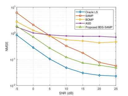
Figure 5: NMSE performance comparison of different channel estimation schemes for SNS massive MIMO systems ($P_{h}$ = 32, $P_{v}$ = 32, $K$ = 256, $\rho=0.45$).

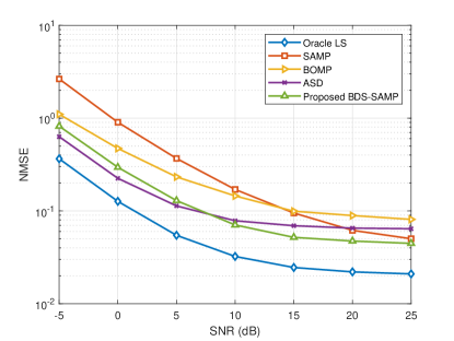
Figure 6: NMSE performance comparison of different channel estimation schemes for SS massive MIMO systems ($P_{h}$ = 32, $P_{v}$ = 32, $K$ = 256, $\rho=0$).

Fig. 5 shows the NMSE performance of the proposed DBS-SAMP scheme with $P_{h}$ = 32, $P_{v}$ = 32, $K$ = 256, and $\rho=0.45$. For comparison, the results of oracle LS [17], SAMP scheme, BOMP scheme [12], and ASD scheme [16] are also given. It can be seen that the proposed BDS-SAMP scheme can achieve obvious improvement in accuracy compared with SAMP, BOMP, and ASD, especially in high SNR region. This is mainly due to the adaptively estimation of beam dominant terms on the basis of channel structure and the presetting of power leakage. Compared with SAMP, the proposed BDS-SAMP scheme can achieve higher estimation accuracy with the similar complexity. At SNR=20 dB, the result of BDS-SAMP scheme has more than 20% improvement than that of SAMP. The oracle LS can directly select the dominant beam supports according to the known sparsity, which is an ideal estimate that can be regarded as the performance upper boundary. The ASD estimation scheme assumes that the sparsity is known, and the range of the beam domain dominant terms is adjusted in the form of rectangular-blocks. Therefore, the estimation performance of ASD may be better when SNR = -5 dB. However, when the number of beams in SNS channel increases, the performance of ASD estimation decreases with the increase of SNR compared with the proposed BDS-SAMP. Besides, since SNS channels are not regular sparse blocks, simply using BOMP to divide the channel into regular blocks will inevitably lead to poor estimation performance. Furthermore, since $K$ is much smaller than the dimension of beam domain channel $P$ = 1024, the proposed scheme has low pilot overhead.

Fig. 6 shows the beam domain channel estimation performance of the proposed scheme with $P_{h}$ = 32, $P_{v}$ = 32, $K$ = 256, and $\rho=0$ for SS massive MIMO systems. It is clear that the estimation performance of SS channel is generally better than that of SNS channel, but this comes at the cost of channel authenticity. In this case, the proposed BDS-SAMP scheme can perform better in accuracy compared with SAMP, BOMP, and ASD, especially in high SNR region. Besides, the performance of BDS-SAMP is similar to that of ASD in low SNR region. This is mainly because the rectangular-blocks beam structure used by ASD covers the cross-blocks used by BDS-SAMP in the case of low SNR for SS channel.

Fig. 7 displays the NMSE performance of the proposed scheme for different sizes of UPA, i.e., 32$\times$32, 48$\times$48, and 64$\times$64. It is shown that the performance of NMSE improves with increasing the size of antennas both in low and high SNR regions. This is because the power leakage is more severe for larger antenna array with a given VR length. Fig. 5, Fig. 6, and Fig. 7 fully illustrate the accuracy and robustness of the proposed algorithm for massive MIMO channel estimation.

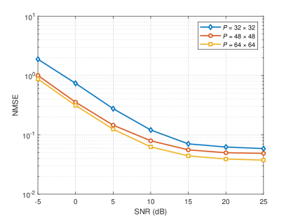
Figure 7: NMSE performance comparison for different sizes of UPA ($K=P/4$, $\rho=0.45$).

VI Conclusions

In this paper, a BDS-SAMP channel estimation scheme for massive MIMO BDCM concerning the spatial non-stationarity and power leakage has been proposed. To evaluate our scheme, a realistic massive MIMO BDCM has been adopted to capture spatial non-stationarity. The sparse structure and power leakage effect have been further demonstrated. Based on the cross-block sparse structure and power ratio threshold of beam domain channel, the beam support set has been iteratively obtained in BDS-SAMP channel estimation scheme. The simulation results have validated the accuracy and effectiveness of the proposed scheme. The proposed BDS-SAMP scheme can achieve obvious improvement in accuracy compared with SAMP, BOMP, and ASD for SNS massive MIMO systems. What’s more, when the number of antennas increases, the proposed scheme can perform well for massive MIMO systems.

References

- [1] C.-X. Wang, J. Huang, H. Wang, et al., “6G wireless channel measurements and models: Trends and challenges,” IEEE Veh. Technol. Mag., vol. 15, no. 4, pp. 22–32, Dec. 2020.
- [2] C.-X. Wang, X.-H. You, X. Gao, et al., “On the road to 6G: Visions, requirements, key technologies and testbeds,” IEEE Commun. Surveys Tuts., vol. 25, no. 2, pp. 905–974, 2nd Quart., 2023.
- [3] C.-X. Wang, Z. Lv, X. Gao, et al., “Pervasive wireless channel modeling theory and applications to 6G GBSMs for all frequency bands and allscenarios,” IEEE Trans. Veh. Technol., vol. 71, no. 9, pp. 9159–9173, Sept. 2022.
- [4] X.-H. You, C.-X. Wang, J. Huang, et al., “Towards 6G wireless communication networks: Vision, enabling technologies, and new paradigm shifts,” Sci. China Inf. Sci., vol. 64, no. 1, pp. 1–74, Jan. 2020.
- [5] J. Bian, C.-X. Wang, R. Feng, et al., “A novel 3D beam domain channel model for massive MIMO communication systems,” IEEE Trans. Wireless Commun., vol. 22, no. 3, pp. 1618–1632, Mar. 2023.
- [6] M. Sayeed, “Deconstructing multiantenna fading channels,” IEEE Trans. Signal Process., vol. 50, no. 10, pp. 2563–2579, Oct. 2002.
- [7] D. L. Donoho, “Compressed sensing,” IEEE Trans. Inform. Theory, vol. 52, no. 4, pp. 1289–1306, Apr. 2006.
- [8] X. Lin, S. Wu, L. Kuang, et al., “Estimation of sparse massive MIMO-OFDM channels with approximately common support,” IEEE Commun. Lett., vol. 21, no. 5, pp. 1179–1182, May 2017.
- [9] C. Chen and M. D. Zoltowski, “Bayesian sparse channel estimation and tracking,” in Proc. SSP’12, Ann Arbor, MI, USA, Aug. 2012, pp. 472–475.
- [10] Y. Huang, Y. He, Q. Luo, L. Shi, and Y. Wu, “Channel estimation in MIMO–OFDM systems based on a new adaptive greedy algorithm,” IEEE Wireless Commun. Lett., vol. 8, no. 1, pp. 29–32, Feb. 2019.
- [11] Z. Gao, L. Dai, Z. Wang, and S. Chen, “Spatially common sparsity based adaptive channel estimation and feedback for FDD massive MIMO,” IEEE Trans. Signal Process., vol. 63, no. 23, pp. 6169–6183, Dec. 2015.
- [12] X. Ma, F. Yang, S. Liu, J. Song, and Z. Han, “Sparse channel estimation for MIMO-OFDM systems in high-mobility situations,” IEEE Trans. Vehi. Technol., vol. 67, no. 7, pp. 6113–6124, July 2018.
- [13] Y. Zheng, C.-X. Wang, R. Yang, et al., “6G ultra-massive MIMO channel measurements at 5.3 GHz and a general channel model,” IEEE Trans. Veh. Technol., vol. 72, no. 1, pp. 20–34, Jan. 2023.
- [14] J. Chen, P. Zhang, N. Ma, and X. Xu, “Hierarchical-block sparse Bayesian learning for spatial non-stationary massive MIMO channel estimation,” IEEE Wireless Commun. Lett., vol. 11, no. 5, pp. 888–892, May 2022.
- [15] S. Hou, Y. Wang, T. Zeng, and S. Wu, “Sparse channel estimation for spatial non-stationary massive MIMO channels,” IEEE Commun. Lett., vol. 24, no. 3, pp. 681–684, Mar. 2020.
- [16] X. Gao, L. Dai, S. Han, I. Chih-Lin, and F. Adachi, “Beamspace channel estimation for 3D lens-based millimeter-wave massive MIMO systems,” in Proc. IEEE WCSP’16, Yangzhou, China, Oct. 2016, pp. 1–5.
- [17] X. Gao, L. Dai, S. Zhou, A. M. Sayeed, and L. Hanzo, “Wideband beamspace channel estimation for millimeter-wave MIMO systems relying on lens antenna arrays,” IEEE Trans. Signal Process., vol. 67, no. 18, pp. 4809–4824, Sept. 2019.
- [18] X. Gao, L. Dai, S. Han, C.-L. I, and X. Wang, “Reliable beamspace channel estimation for millimeter-wave massive MIMO systems with lens antenna array,” IEEE Trans. Wireless Commun., vol. 16, no. 9, pp. 6010–6021, Sept. 2017.
- [19] H. Chang, C.-X. Wang, J. Bian, et al., “A novel 3D beam domain channel model for UAV massive MIMO communications,” IEEE Trans. Wireless Commun., vol. 22, no. 8, pp. 5431–5445, Aug. 2023.
- [20] W. Ma and C. Qi, “Channel estimation for 3-D lens millimeter wave massive MIMO system,” IEEE Commun. Lett., vol. 21, no. 9, pp. 2045–2048, Sept. 2017.
- [21] J. Gholipour, K. L. Bober, M. Hinrichs and V. Jungnickel, “Compressed Sensing for Feedback Generation in OFDM Based LiFi Systems,”in Proc. IEEE WCNC’23 , Glasgow, United Kingdom, 2023, pp. 1-6.
- [22] 3GPP, Tech. Rep. 38.901, “Study on channel model for frequencies from 0.5 to 100 GHz (Release 14),” Mar. 2017.