A Support Vector Approach in Segmented Regression for Map-assisted Non-cooperative Source Localization

Abstract

This paper presents a non-cooperative source localization approach based on received signal strength (RSS) and 2D environment map, considering both line-of-sight (LOS) and non-line-of-sight (NLOS) conditions. Conventional localization methods, e.g., weighted centroid localization (WCL), may perform bad. This paper proposes a segmented regression approach using 2D maps to estimate source location and propagation environment jointly. By leveraging topological information from the 2D maps, a support vector-assisted algorithm is developed to solve the segmented regression problem, separate the LOS and NLOS measurements, and estimate the location of source. The proposed method demonstrates a good localization performance with an improvement of over 30% in localization rooted mean squared error (RMSE) compared to the baseline methods.

I Introduction

Non-cooperative localization [1, 2] finds important applications in real-world scenarios. In communication networks, accurate localization of node failures plays a crucial role in maintaining network resilience and enhancing operational efficiency [3]. In modern power systems, rapid and precise localization of attacks or disturbances is essential for safeguarding grid stability and ensuring uninterrupted service [4]. In cognitive radio networks, reliable spectrum sensing enables secondary users to locate and access available spectrum without interfering with primary users [5]. In these scenarios, it is difficult to perform localization that requires cooperation among nodes. For example, measuring the time of arrival (TOA) or time difference of arrival (TDOA) require pilot sequences or preambles for an accurate estimation of the timing of the received signal. By contrast, RSS or angle of arrival (AoA) based methods can detect and localize non-cooperative sources, because they do not require the preamble or data of the signal source, but rely on fitting the statistics of the received signal to the propagation model.

However, RSS or AoA based methods [6, 7] suffer from poor localization accuracy. To begin with, these methods require an empirical propagation model, but the model parameters may not be accurately known by the system. In addition, as the signal strength decreases substantially as the distance increases, a small fluctuation in signal strength, due to multi-paths or shadowing, can be translated to a huge difference in the ranging result. For AoA based methods, the accuracy of the AoA estimation depends on the antenna array configuration and the angular spread of the signals due to the multi-paths. Furthermore, these methods are significantly affected by NLOS propagation, which induces huge fluctuation in signal strength and the spread of AoA.

Leveraging the topological structure of radio maps can enable the localization of a non-cooperative signal source without relying on accurate propagation models. Here, radio maps refer to the spatial distribution of the RSS of the signal emitted from the source location. Thus, reversely, one can leverage the RSS patterns and the spatial relationship with the geometric layout of the propagation environment to infer the location of the signal source. A common scenario is to collect the RSS of a signal source by a group of measurements scattered at various locations. A simplest approach to estimate the source location is to use the WCL algorithm, which estimates the source location as the weighted sum of the sensor locations using the RSS as the weights [8, 9, 10]. Another non-parametric approach is to use matrix or tensor models for radio map representation [11, 12, 13], where a radio map is first reconstructed using sparse matrix completion, and then, the source is localized by extracting some feature vectors from matrix factorization. Furthermore, when there is NLOS, one can jointly reconstruct the environment and the radio map [14, 15], and by knowing the location of propagation obstacle, a substantially better RSS-based localization performance can be achieved [16, 14].

It is not surprising that exploiting 3D environment map can enhance RSS-based localization, as the subset of RSS measurements can be identified based on the 3D map. However, as an accurate 3D environment map is more difficult to obtain compared to its 2D counterpart, it is important to understand how to localize a source using 2D environment maps. The main challenge is whether we need to jointly source location and the heights of the obstacles for a classification of LOS and NLOS. This paper finds that it is not necessary to reconstruct the heights of the obstacles for map-assisted RSS-based source localization. Instead, we develop a support vector method to exploit the information from a 2D environment map. Specifically, we exploit the geometric property of the propagation environment and formulate a segmented regression problem to learn the spatial feature of the radio map. We develop a support vector-assisted approach to solve the segmented regression problem. We demonstrate that the proposed method offers a reliable and effective solution for localization, maintaining high accuracy across different number of measurements and variable shadowing conditions and achieving a reduction in localization RMSE of over $30$% compared to baseline methods, making it well-suited for practical applications requiring precise localization.

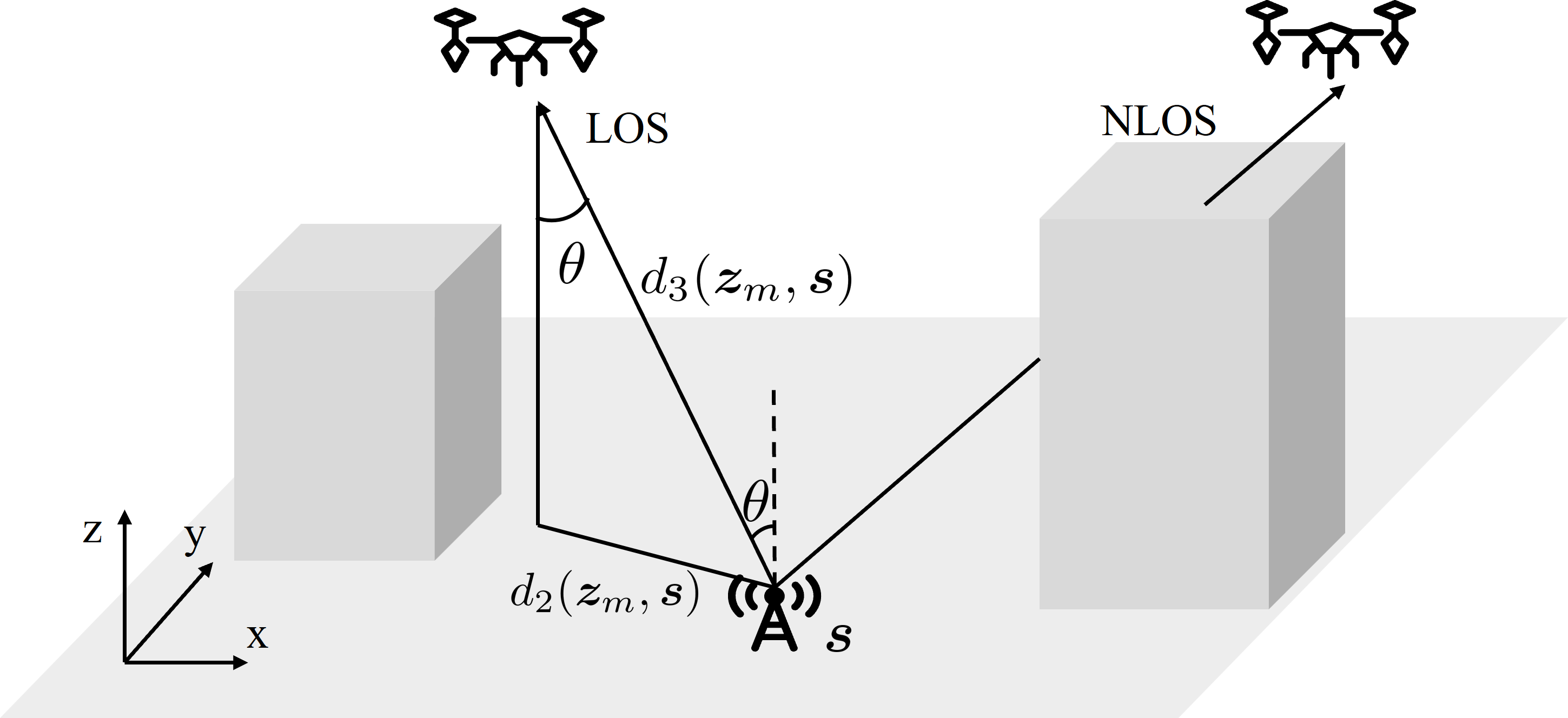
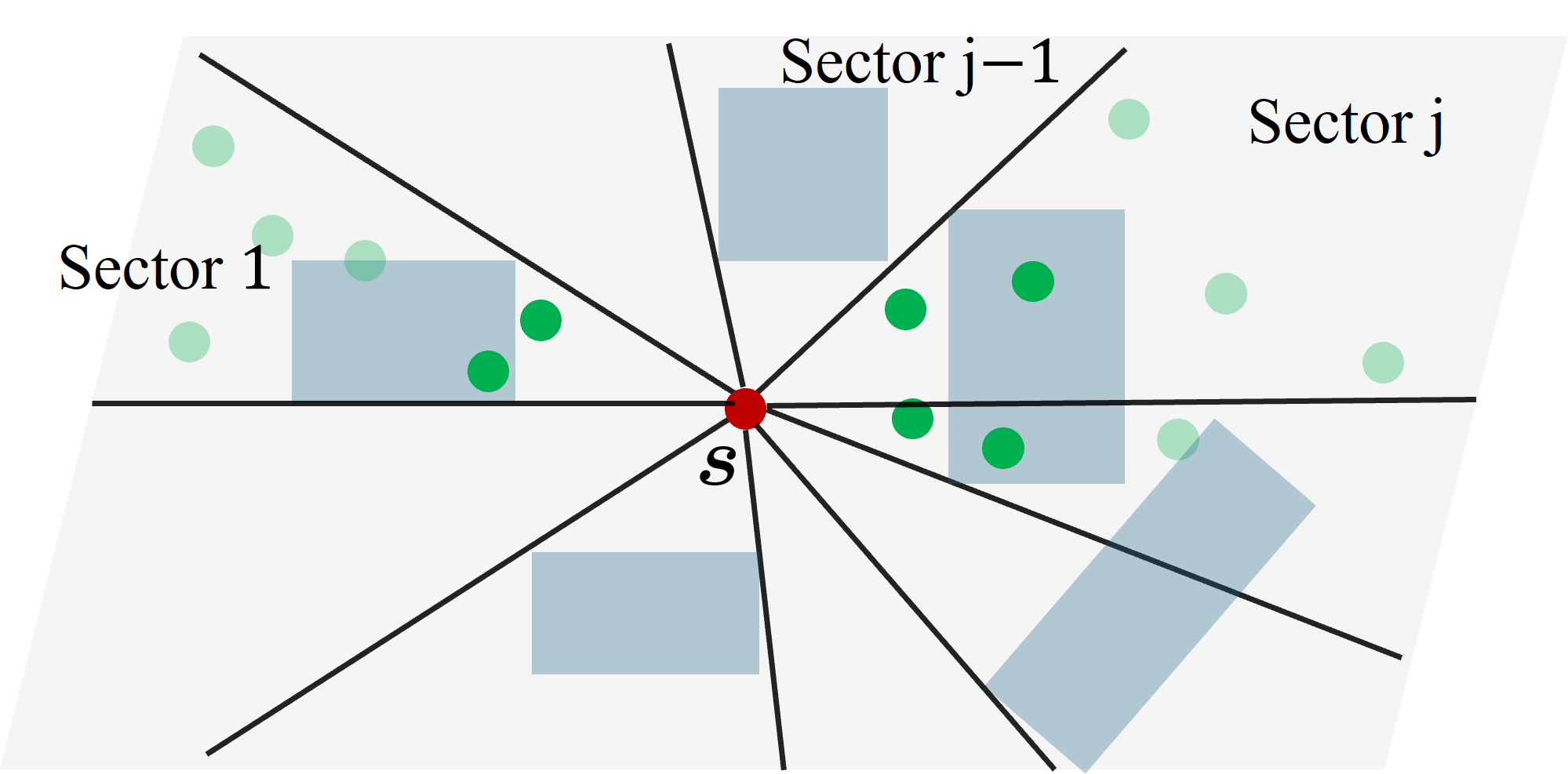
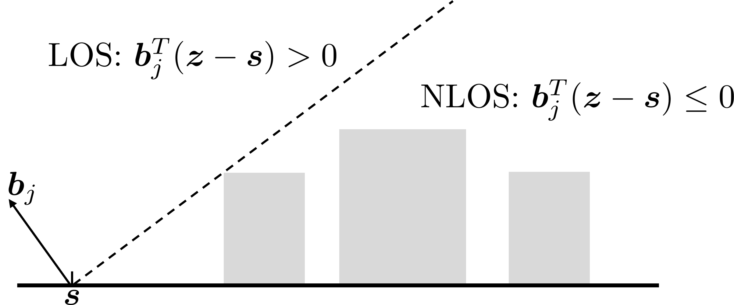
Figure 1: (a) A signal source is located on the ground, and a UAV flies through the air to collect the RSS, with both LOS and NLOS conditions present. (b) Sectors partition. Sector $j$ serves as an example. The red circle represents the presumed source location $\bm{s}$, the blue rectangular represents the buildings, the dark green circle represents measurements under LOS conditions, and the light green circle represents measurements under NLOS conditions. (c) Support vector $\bm{b}_{j}$ and the separation between LOS and NLOS conditions.

II System Model

Consider a blockage environment with a hidden signal source on the ground at $\bm{s}\in\mathbb{R}^{3}$ to be localized as depicted in Fig. 1 (a). The locations of the propagation obstacles are available, but the heights of the obstacles are unknown. Thus, the blockage status for the measurement locations at some regions is not immediately available.

Consider a set of measurements $y_{m}$ collected at different locations $\bm{z}_{m}\in\mathbb{R}^{3}$, $m=1,2,\dots,M$, where the $m$th measurement location can be attained by an aerial node above the ground. In general, the measurement $y_{m}$ can be a vector if the receiver equips an antenna array or has the capability to identify multipaths. For the ease of elaboration, we simply consider $y_{m}\in\mathbb{R}$ measures the RSS of the signal emitted from unknown location.

II-A Radio Map Model

Since there is possible blockages, denote $\mathcal{D}_{0}\subset\mathbb{R}^{6}$ as the LOS propagation region for the receiver at location $\bm{z}\in\mathbb{R}^{3}$ and the signal source at $\bm{s}\in\mathbb{R}^{6}$. Likewise, $\mathcal{D}_{1}\subset\mathbb{R}^{6}$ denotes the NLOS propagation region. The radio map for each receiver and signal source pair $(\bm{z},\bm{s})\in\mathbb{R}^{6}$ is modeled as follows:

$$f(\bm{z},\bm{s};\bm{\Phi}) =\begin{cases}f_{0}(\bm{z},\bm{s};\bm{\phi}_{0})+\epsilon_{0}&(\bm{z},\bm{s})\in\mathcal{D}_{0}\\ f_{1}(\bm{z},\bm{s};\bm{\phi}_{1})+\epsilon_{1}&(\bm{z},\bm{s})\in\mathcal{D}_{1}\end{cases}$$ (1)

where $\epsilon_{k}$, $k=0,1$ is a random variable to capture the shadowing due to signal blockage, reflection and diffraction, etc, and $\epsilon_{0}\sim\mathcal{N}(0,\sigma_{0}^{2})$, $\epsilon_{1}\sim\mathcal{N}(0,\sigma_{1}^{2})$, $\bm{\Phi}=\{\mathcal{D}_{0},\mathcal{D}_{1},\bm{\phi}_{0},\bm{\phi}_{1}\}$ is a collection of the radio map parameters. The functions $f_{0}(\bm{z},\bm{s};\bm{\phi}_{0})$ and $f_{1}(\bm{z},\bm{s};\bm{\phi}_{1})$ represent the propagation models with parameters $\bm{\phi}_{0}$ and $\bm{\phi}_{1}$, corresponding to LOS and NLOS, respectively, and these models can be represented by a neural network, a non-parametric model, or a parametric model according to the application scenario to be specified later.

The aim of the model (1) is to decompose the radio map model into the component $\{\mathcal{D}_{0},\mathcal{D}_{1}$}, which captures the LOS and NLOS patterns, and the component $\{f_{0},f_{1}\}$, which captures the propagation law affected by unknown factors, including power and antenna configurations. The radio map approach thus aims at localizing the source location without explicitly recovering these propagation factors. A general localization problem can be formulated as follows:

$$\underset{\bm{s},\bm{\text{$\Phi$}}}{\text{minimize}}\sum_{m}(y_{m}-f(\bm{z}_{m},\bm{s};\bm{\Phi}))^{2}.$$

The problem is to find a source location $\bm{s}$ such that the corresponding radio map $f(\bm{z}_{m},\bm{s};\bm{\Phi})$ for the source at $\bm{s}$ matches with the measurements $\{(\bm{z}_{m},y_{m})\}$.

II-B Segmented Propagation with Support Vectors

It is challenging to specify the propagation regions $\mathcal{D}_{0}$ and $\mathcal{D}_{1}$, because they can appear with an arbitrary shape. However, when the obstacle location is available, the propagation region can be specified using support vectors that can be learned from the measurements $\{(\bm{z}_{m},y_{m})\}$.

II-B1 Sectoring of Measurements

Suppose that we are given a source location $\bm{s}$. Then, on a top view, the area can be partitioned into $J(\bm{s})$ sectors centered at $\bm{s}$, where these sectors approximately separate the obstacles from each other as much as possible according to $\bm{s}$ as depicted in Fig. 1 (b). Then, the measurements can be clustered to different index set $\mathbb{M}_{j}(\bm{s})$ according to $\bm{s}$ where $j$ corresponds to the sector.

In practice, sectorization is a challenging task in a complex environment. However, in our specific application as shown in Fig. 1 (c) to be discussed later, there is only one building in each direction that plays a critical role in determining the boundary of LOS and NLOS regions, and this critical building, empirically, usually locates nearby the source location $\bm{s}$. As a result, one can approximately perform sectorization based on a few buildings near the source location $\bm{s}$, although the building heights are assumed unknown. Note that the sectorization depends on the presumed source location $\bm{s}$, and hence, it needs to be updated with the localization algorithm discussed later.

II-B2 Support Vectors and Regression Model

The advantage of the sectoring is that for each sector $j$, the LOS region can be determined by a linear operation with a support vector $\bm{b}_{j}$ as depicted in Fig. 1 (c) from a horizontal view. Mathematically, given a presumed source location $\bm{s}$ and defining a normal vector $\bm{b}_{j}$ of the LOS-NLOS separating plane, the LOS region in the $j$th sector is the set of locations $\bm{z}$ such that $\bm{b}_{j}^{\text{T}}(\bm{z}-\bm{s})>0$, and the NLOS region in the $j$th sector is the set of locations $\bm{z}$ such that $\bm{b}_{j}^{\text{T}}(\bm{z}-\bm{s})\leq 0$.

As a result, the radio map model parameter $\bm{\Phi}$ can be simplified to $\bm{\Phi}=\{\{\bm{b}_{j}\},\bm{\phi}_{0},\bm{\phi}_{1}\}$, which depends on the presumed source location $\bm{s}$ to be optimized. The source localization problem becomes a joint segmented regression problem assisted by support vectors:

$$\underset{\bm{s},\bm{\phi}_{k},\{\bm{b}_{j}\}}{\text{minimize}} \quad\sum_{j=1}^{J(\bm{s})}\sum_{m\in\mathbb{M}_{j}(\bm{s})}(y_{m}-\sum_{k=0}^{1}f_{k}(\bm{z}_{m},\bm{s};\bm{\phi}_{k}))^{2}u_{m}^{(k)}$$ (2)

subject to $$\quad u_{m}^{(k)}=\mathbb{I}_{k}(\bm{z}_{m},\bm{s},\bm{b}_{j}),k=0,1$$

where $u_{m}^{(k)}$ are auxiliary variables to classify measurements locations $\bm{z}_{m}$ into LOS regions or NLOS regions according to the support vectors $\bm{b}_{j}$, and

$$\mathbb{I}_{k}(\bm{z}_{m},\bm{s},\bm{b}_{j})=\begin{cases}\mathbb{I}(\bm{b}_{j}^{\text{T}}(\bm{z}_{m}-\bm{s})\geq 0)&\text{if}\ k=0\\ \mathbb{I}(\bm{b}_{j}^{\text{T}}(\bm{z}_{m}-\bm{s})<0)&\text{if}\ k=1\end{cases}$$

and $\mathbb{I}(x)$ is an indicator function with $\mathbb{I}(x)=1$ if $x$ is true, and $\mathbb{I}(x)=0$, otherwise.

III Segmented Regression for Localization

In this section, we consider a scenario where the source and areal nodes all equipped with antennas for signal transmission and reception. We propose a parametric model to represent the radio map. The parametric model can vary with different types of antennas. Then, we propose a segmented regression method to fit the measurements to the parametric model to account for both LOS and NLOS conditions, which are affected by the obstruction of buildings. Finally, the source location is estimated by identifying the presumed location where the regression residual is minimized.

III-A Parametric Model to Represent $f(\bm{z},\bm{s};\bm{\bm{\Phi}})$

We propose a parametric model $\rho_{k}(\bm{z},\bm{s};\bm{\phi}_{k})$ to approximate the radio map model $f(\bm{z},\bm{s};\bm{\bm{\Phi}})$ in (1) as follows:

$$\rho_{k}(\bm{z},\bm{s};\bm{\phi}_{k}) =a_{k}+b_{k}\log(d_{3}(\bm{z},\bm{s}))+c_{k}\text{log}(d_{2}(\bm{z},\bm{s}))+\epsilon_{k}$$ (3)

where $\bm{\phi}_{k}=[a_{k},b_{k},c_{k}]$.

Note that the parametric form in (3) is universal in modeling wireless propagation channels. For example, considering a classical empirical channel model in the linear scale

$$y(\bm{z})=\begin{cases}Pg_{0}(d_{3}(\bm{z},\bm{s}))g(\theta(\bm{z},\bm{s}))+\epsilon_{0}&(\bm{z},\bm{s})\in\mathcal{D}_{0}\\ Pg_{1}(d_{3}(\bm{z},\bm{s}))g(\theta(\bm{z},\bm{s}))+\epsilon_{1}&(\bm{z},\bm{s})\in\mathcal{D}_{1}\end{cases}$$ (4)

where $P$ is the transmitted power,

$$g_{k}(d_{3}(\bm{z},\bm{s}))=(d_{3}(\bm{z},\bm{s}))^{-\beta_{k}}$$ (5)

is the path loss and $g(\theta(\bm{z},\bm{s}))$ is the radiation pattern of the antenna. The transmitted power $P$ corresponds to the first term $a_{k}$ in (3). The path loss model in the log-scale can be written as $\beta_{k}\log(d_{3}(\bm{z},\bm{s}))$ which corresponds to part of the second term $b_{k}\log(d_{3}(\bm{z},\bm{s}))$ in (3).

For the antenna radiation pattern $g(\theta(\bm{z},\bm{s}))$, we take a vertically polarization antenna as an example. The antenna gain is modeled as [17]:

$$g(\theta(\bm{z},\bm{s}))=\text{cos}(\frac{\pi}{2}\text{cos}(\theta(\bm{z},\bm{s})))^{2}\approx\text{\text{sin}}^{5}(\theta)$$

where $\text{\text{sin}}(\theta)=d_{2}(\bm{z},\bm{s})/d_{3}(\bm{z},\bm{s})$, $d_{3}(\bm{z},\bm{s})=\|\bm{z}-\bm{s}\|_{2}$ is the distance from the aerial node $\bm{z}$ to source location $\bm{s}$ in 3D, where $\|\cdot\|_{2}$ denotes $l_{2}$ norm, $d_{2}(\bm{z},\bm{s})$ captures the distance between the aerial node $\bm{z}$ and source location $\bm{s}$ in 2D without considering the height, and $\text{log}(\text{sin}(\theta))=-\log(d_{3}(\bm{z},\bm{s}))-\text{log}(d_{2}(\bm{z},\bm{s}))$. As a result, under the log-scale, the antenna pattern corresponds to the third term $c_{k}\text{log}(d_{2}(\bm{z},\bm{s}))$ and part of the second term $b_{k}\log(d_{3}(\bm{z},\bm{s}))$ in (3).

As seen from the above examples, the parametric form $\rho_{k}(\bm{z},\bm{s};\bm{\phi}_{k})$ is very general, not assuming too much information about the device, power budget, environment, or propagation pattern.

III-B Segmented Regression for LOS and NLOS Measurements Separation

In this subsection, we estimate the support vector $\bm{b}_{j}$ for the separation of LOS and NLOS measurements in sector $j$. According to the 2D environment map and location $\bm{s}$, the measurements can be partitioned into totally $J(\bm{s})$ sectors. The measurements in the same sector have a consistent blocking condition, i.e., for the measurements satisfy $\bm{b}_{j}(\bm{z}_{m}-\bm{s})>0$, the LOS condition exists, otherwise NLOS condition exists.

We propose to estimate $\bm{b}_{j}$ through minimizing the segmented regression residual.

The model $\rho_{k}^{(j)}(\bm{z}_{m},\bm{s};\bm{\phi}_{k})$ at $j$th sector part is the same as $\rho_{k}(\bm{z}_{m},\bm{s};\bm{\phi}_{k})$ in (3), since the parameters $a_{k}$, $b_{k}$, $c_{k}$ are independent of sector $j$ and only $\bm{b}_{j}$ is different. Then, the parametric model $\rho_{k}$ and support vector $\bm{b}_{j}$ at sector $j$ can be estimated through solving

$$\underset{\bm{\phi},\bm{b}_{j}}{\text{mininize}} \quad\sum_{m\in\mathbb{M}_{j}(\bm{s})}(y_{m}-\sum_{k=0}^{1}\rho_{k}(\bm{z}_{m},\bm{s};\bm{\bm{\phi}}_{k}))^{2}u_{m}^{(k)}$$ (6)

subject to $$\quad u_{m}^{(k)}=\mathbb{I}_{k}(\bm{z}_{m},\bm{s},\bm{b}_{j}),k=0,1.$$

For the convenience of calculation, the matrix form of (6) is formulated as follows:

$$\underset{\bm{\phi},\bm{b}_{j}}{\text{min}}\quad\|\bm{y}_{j}-\tilde{\bm{D}}^{\text{T}}\bm{\phi}\|_{2}^{2}$$ (7)

where $\bm{y}_{j}\in\mathbb{R}^{|\mathbb{M}_{j}(\bm{s})|\times 1}$ is a vector containing all measurements $y_{m}$ for $m\in\mathbb{M}_{j}(\bm{s})$, $\mathbb{M}_{j}(\bm{s})$ represents the set of measurement indices in sector $j$, $|\mathbb{M}_{j}(\bm{s})|$ denotes the number of elements in $\mathbb{M}_{j}(\bm{s})$, $\mathbb{M}_{j,i}$ denotes the $i$th index in $\mathbb{M}_{j}(\bm{s})$, $\bm{\phi}=[\bm{\phi}_{0};\bm{\phi}_{1}]\in\mathbb{R}^{6\times 1}$, $\tilde{\bm{D}}=[\bm{x}_{\mathbb{M}_{j,1}}\circ\bm{I}_{\mathbb{M}_{j,1}};\cdots;\bm{x}_{\mathbb{M}_{j,|\mathbb{M}_{j}(\bm{s})|}}\circ\bm{I}_{\mathbb{M}_{j,|\mathbb{M}_{j}(\bm{s})|}}]\in\mathbb{R}^{6\times|\mathbb{M}_{j}(\bm{s})|}$, $\bm{x}_{\mathbb{M}_{j,i}}=[\bm{D}_{\mathbb{M}_{j,i}};\bm{D}_{\mathbb{M}_{j,i}}]\in\mathbb{R}^{6\times 1}$, $\bm{D}_{\mathbb{M}_{j,i}}=[1,\text{log}(d_{3}(\bm{z}_{\mathbb{M}_{j,i}},\bm{s})),\text{log}(d_{2}(\bm{z}_{\mathbb{M}_{j,i}},\bm{s}))]^{\text{T}}\in\mathbb{R}^{3\times 1}$, $\bm{I}_{\mathbb{M}_{j,i}}=[u_{\mathbb{M}_{j,i}}^{(0)};u_{\mathbb{M}_{j,i}}^{(0)};u_{\mathbb{M}_{j,i}}^{(0)};u_{\mathbb{M}_{j,i}}^{(1)};u_{\mathbb{M}_{j,i}}^{(1)};u_{\mathbb{M}_{j,i}}^{(1)}]^{\text{T}}\in\mathbb{R}^{6\times 1}$, and ‘$\circ$’ represents element-wise product.

Problem (7) is unconstrained least-squares problem, and it is convex with respect to (w.r.t.) $\bm{\phi}$. It can be solved by setting the derivative to zero, and the solution is given by:

$$\hat{\bm{\phi}}_{j}=(\tilde{\bm{D}}\tilde{\bm{D}}^{\text{T}})\tilde{\bm{D}}\bm{y}_{j}.$$

Noted that the parameter $\bm{b}_{j}$ is unknown, we propose to estimate $\bm{b}_{j}$ based on the residual of regression in (7). More specifically, under fixed $\bm{s}$, each value of $\bm{b}_{j}$ corresponding to a residual $\|\bm{y}_{j}-\tilde{\bm{D}}^{\text{T}}\hat{\bm{\phi}}_{j}\|_{2}^{2}$, and the optimal $\bm{b}_{j}$ is obtained when the residual $\|\bm{y}_{j}-\tilde{\bm{D}}^{\text{T}}\hat{\bm{\phi}}_{j}\|_{2}^{2}$ is minimized.

III-C Localization via Regression Residual Minimization

In this subsection, under each presumed $\bm{s}$, we solve $J(\bm{s})$ segmented regression problems together and calculate the residuals. The location of the source is the one with the smallest regression residual.

We propose to solve $J(\bm{s})$ segmented regressions altogether as follows:

$$\underset{\bm{\phi},\{\bm{b}_{j}\},\bm{s}}{\text{min}} \quad\sum_{j=1}^{J(\bm{s})}\sum_{m\in\mathbb{M}_{j}(\bm{s})}(y_{m}-\sum_{k=0}^{1}\rho_{k}(\bm{z}_{m},\bm{s};\bm{\phi}_{k}))^{2}u_{m}^{(k)}$$ (8)

subject to $$\quad u_{m}^{(k)}=\mathbb{I}_{k}(\bm{z}_{m},\bm{s},\bm{b}_{j}),k=0,1.$$

Similarly to (7), the matrix form of (8) is formulated as follows:

$$\underset{\bm{\phi},\{\bm{b}_{j}\},\bm{s}}{\text{min}}\sum_{j=1}^{J(\bm{s})}\|\bm{y}_{j}-\tilde{\bm{D}}^{\text{T}}\bm{\phi}\|_{2}^{2}.$$ (9)

We propose to solve problem (9) using alternating minimization method. In problem (9), when the parameter $\{\bm{b}_{j}\}$ and $\hat{\bm{s}}$ is the ground truth that match with the scenario, then, the solution $\hat{\bm{\phi}}$ will obtain the optimal value and the residual $\sum_{j=1}^{J(\bm{s})}\|\bm{y}_{j}-\tilde{\bm{D}}^{\text{T}}\hat{\bm{\phi}}\|_{2}^{2}$ will attain the smallest value. A visual plot of the regression residual w.r.t. to the location is shown in Fig. 2,

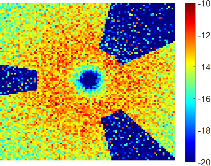
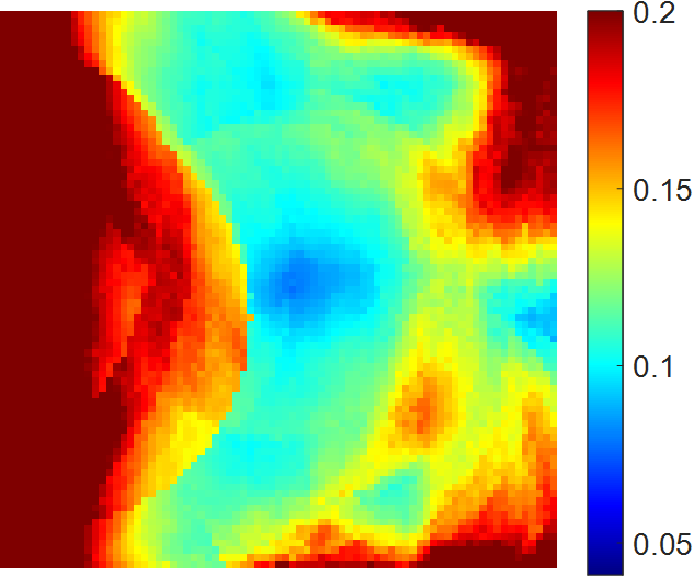
Figure 2: The location of the source corresponds to the location of the smallest regression residual. (a) The radio map. (b) The regression residual versus location $\bm{s}$.

the location with smallest residual corresponds to the location of the source. Thus, we propose to estimate $\{\hat{\bm{b}}_{j}\}$ and $\hat{\bm{s}}$, through minimizing the residuals.

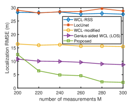
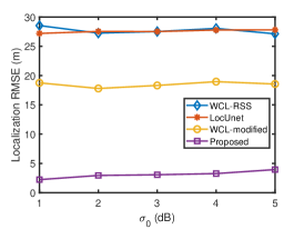
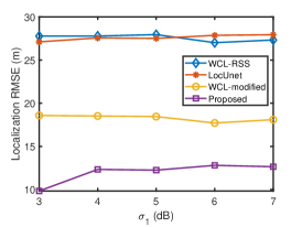
Figure 3: (a) Localization RMSE versus number of sensors. (b) Localization RMSE versus shadowing component $\epsilon_{0}$ under $\sigma_{0}=1-5$ dB, $\sigma_{1}=3$dB, $M=200$. (c) Localization RMSE versus shadowing component $\epsilon_{1}$ under $\sigma_{0}=3$dB, $\sigma_{1}=3-7$ dB, $M=200$.

Update of $\hat{\bm{s}}$ and $\hat{\bm{b}}_{j}$: We propose an exhaustive searching method to find the optimal $\hat{\bm{s}}$ and $\{\hat{\bm{b}}_{j}\}$ that contribute to the smallest residuals. For each presumed $\bm{s}$ and $\bm{b}_{j}$, the residual is obtained by $r(\bm{s},\bm{b}_{j})=\|\bm{y}_{j}-\tilde{\bm{D}}^{\text{T}}\hat{\bm{\phi}}_{j}\|_{2}^{2}$. We can vary all the possible $N_{s}$ values of $\bm{s}$ and $N_{b}$ values of each $\bm{b}_{j}$, and construct an error tensor $\bm{\mathcal{E}}\in\mathbb{R}^{N_{s}\times N_{b}\times J(\bm{s})}$. Then, we extract an error matrix $\bm{E}_{n_{s}}\in\mathbb{R}^{N_{b}\times J(\bm{s})}$ from $\bm{\mathcal{E}}$ where $\bm{E}_{n_{s}}=\bm{\mathcal{E}}(n_{s},:,:)$, $n_{s}=1,\dots,N_{s}$ which represents the error under $n_{s}$th presumed source $\bm{s}$. The error vector $\bm{E}_{n_{s}}(:,j)$ represents the error under $n_{s}$th source and $j$th sector via varying the value of $\bm{b}_{j}$. The index of the smallest value in $\bm{E}_{n_{s}}(:,j)$ corresponds to the optimal value $\hat{\bm{b}}_{j}$.

For each source index $n_{s}$, we calculate its corresponding error summation as $e_{n_{s}}=\sum_{j=1}^{J(\bm{s})}\text{min}\ \bm{E}_{n_{s}}(:,j)$. The index $n_{s}$ of the smallest $e_{n_{s}}$ corresponds to source location $\hat{\bm{s}}$. Under the index $n_{s}$, the index $j$ of $\text{$\underset{j}{\text{min}}$\ }\bm{E}_{n_{s}}(:,j)$ corresponds to the optimal $\hat{\bm{b}}_{j}$.

Update of $\bm{\phi}$: With the estimated $\hat{\bm{s}}_{j}$ and $\{\hat{\bm{b}}_{j}\}$, solving a global coefficients $\bm{\phi}$ using all the measurements is as follows:

$$\underset{\bm{\phi}}{\text{min}}\|\bm{y}-\bm{\bar{D}}^{\text{T}}\bm{\phi}\|_{2}^{2}$$ (10)

where $\bm{y}=[y_{1},y_{2},\cdots,y_{M}]^{\text{T}}\in\mathbb{R}^{M\times 1}$, $\bm{\phi}=[\bm{\phi}_{0};\bm{\phi}_{1}]\in\mathbb{R}^{6\times 1}$, $\bar{\bm{D}}=[\bm{x}_{1}\circ\bar{\bm{I}}_{1};\cdots;\bm{x}_{M}\circ\bm{\bar{I}}_{M}]\in\mathbb{R}^{6\times M}$, $\bm{x}_{m}=[\bm{D}_{m};\bm{D}_{m}]\in\mathbb{R}^{6\times 1}$, $\bm{D}_{m}=[1,\text{log}(d_{3}(\bm{z}_{m},\bm{s})),\text{log}(d_{2}(\bm{z}_{m},\bm{s}))]^{\text{T}}\in\mathbb{R}^{3\times 1}$, $\bm{\bar{I}}_{m}=[u_{m}^{(0)};u_{m}^{(0)};u_{m}^{(0)};u_{m}^{(1)};u_{m}^{(1)};u_{m}^{(1)}]^{\text{T}}\in\mathbb{R}^{6\times 1}$.

Problem (10) is unconstrained least-squares problem, and can be solved by setting the derivative to zero. The solution is $\hat{\bm{\phi}}=(\bar{\bm{D}}\bm{\bar{D}}^{\text{T}})\bar{\bm{D}}\bm{y}.$

Then, the unknown parameters $\bm{\phi}$, $\{\bm{b}_{j}\}$, $\bm{s}$ in (8) are obtained.

IV Numerical Results

Consider an $L\times L$ area with $L=200$ meters and the aerial nodes are at a height of $h=20$m. Assume the ground source $\bm{s}$ is located at coordinates $(s_{x},s_{y})$. Without loss of generality (w.l.o.g.), we choose $s_{x}=s_{y}=0$. To create LOS and NLOS links, assume there are three buildings around the source. The vertices for Building 1 are $(10,40)$, $(40,20)$, $(30,70)$, and $(60,30)$. For Building 2, the vertices are $(80,-40)$, $(20,-80)$, $(60,-100)$, and $(100,-100)$. For Building 3, the vertices are $(-50,20)$, $(-50,-20)$, $(-70,10)$, and $(-70,-10)$. The aerial nodes collect measurements at $M$ locations, chosen uniformly at random. We utilize the model (3) to generate the RSS collected by the aerial nodes. We choose $\beta_{0}=-2$ and $\beta_{1}=-7$ in (5) and let $P=1$W. The shadowing component follows a Gaussian distribution, $\epsilon_{k}\sim\mathcal{N}(0,\sigma_{k}^{2})$, with $\sigma_{0}=1$ and $\sigma_{1}=5$. We evaluate the localization performance of the proposed method. The criterion for assessment is the localization RMSE, calculated as $\|\hat{\bm{s}}-\bm{s}\|_{2}$, where $\|\cdot\|_{2}$ denotes the $l_{2}$ norm. The performance is benchmarked against four baseline methods. Baseline 1: WCL-RSS: the source location is estimated using the formula $\hat{\bm{s}}=\sum_{m=1}^{M}w(y_{m})\bm{z}_{m}/\sum_{m=1}^{M}w(y_{m})$, where the weight function $w(y_{m})=y_{m}$. Baseline 2: WCL-modified, this method uses the same formula as WCL, but with a modified weight function $w(y_{m})=y_{m}^{0.6}$. Baseline 3: Genius-aided WCL (LOS), this method only uses the LOS measurements to perform localization. Baseline 4: LocUnet [1], in this method, the sparse measurements and 2D environment map are the inputs, while the location of the source is the output.

Fig. 3 (a) illustrates the localization RMSE for varying numbers of measurements $M$ ranging from $200$ to $300$. The shadowing component is chosen as $\sigma_{0}=1$dB, $\sigma_{1}=5$dB. The WCL method demonstrates poor performance due to significant bias, which can arise when measurements are unevenly distributed around the source. Additionally, the presence of NLOS measurements prevents performance improvement as the number of measurements increases. In contrast, the genius-aided WCL (LOS) method relies solely on LOS measurements for localization, resulting in improved performance as the number of measurements grows. The LocUnet method underperforms due to its lack of generalization ability, as the input 2D map has not been adequately trained. In comparison, the proposed method demonstrates superior performance, with a substantial reduction in localization RMSE as the number of measurements increases. This also highlights its ability to effectively separate LOS and NLOS measurements, achieving an improvement of over $80$%.

Fig. 3 (b) illustrates the relationship between localization RMSE and the shadowing component $\epsilon_{0}$ under $\sigma_{0}=1-5$ dB and $\sigma_{1}=3$dB, with $M=200$ measurements. The proposed method demonstrates a significant improvement in performance, achieving over a $60$% reduction in RMSE compared to baseline methods.

Fig. 3 (c) illustrates the relationship between localization RMSE and the shadowing component $\epsilon_{1}$ under $\sigma_{1}=3-7$ dB and $\sigma_{0}=3$dB, with $M=200$ measurements. The proposed method demonstrates a significant improvement in performance, achieving over a $30$% reduction in RMSE compared to baseline methods.

V Conclusion

In conclusion, this work presented a novel segmented regression approach for non-cooperative RSS-based localization utilizing side information from 2D environment maps. The proposed approach leverages topological information, formulates the localization problem as a segmented regression task, and employs a support vector-based solution to effectively estimate the source location, even with limited measurements. The simulation results demonstrated that the proposed method achieves over 30% reduction in localization RMSE compared to baseline methods under various settings.

References

- [1] Ç. Yapar, R. Levie, G. Kutyniok, and G. Caire, “Real-time outdoor localization using radio maps: A deep learning approach,” IEEE Trans. Wireless Commun., vol. 22, no. 12, pp. 9703–9717, 2023.
- [2] H. Sun and J. Chen, “Grid optimization for matrix-based source localization under inhomogeneous sensor topology,” in Proc. IEEE Int. Conf. Acoustics, Speech, and Signal Processing, 2021, pp. 5110–5114.
- [3] L. Ma, T. He, A. Swami, D. Towsley, and K. K. Leung, “Network capability in localizing node failures via end-to-end path measurements,” IEEE/ACM Trans. Netw., vol. 25, no. 1, pp. 434–450, 2017.
- [4] T. R. Nudell, S. Nabavi, and A. Chakrabortty, “A real-time attack localization algorithm for large power system networks using graph-theoretic techniques,” IEEE Trans. Smart Grid, vol. 6, no. 5, pp. 2551–2559, 2015.
- [5] X. Sheng and S. Wang, “Online primary user emulation attacks in cognitive radio networks using thompson sampling,” IEEE Trans. Wireless Commun., vol. 20, no. 12, pp. 8264–8273, 2021.
- [6] Y. Zheng, M. Sheng, J. Liu, and J. Li, “Exploiting AoA estimation accuracy for indoor localization: A weighted AoA-based approach,” IEEE Wireless Commun. Lett., vol. 8, no. 1, pp. 65–68, 2019.
- [7] S. Tomic, M. Beko, and R. Dinis, “3-D target localization in wireless sensor networks using RSS and AoA measurements,” IEEE Trans. Veh. Technol., vol. 66, no. 4, pp. 3197–3210, 2017.
- [8] K. Magowe, A. Giorgetti, S. Kandeepan, and X. Yu, “Accurate analysis of weighted centroid localization,” IEEE Trans. on Cognitive Commun. and Networking, vol. 5, no. 1, pp. 153–164, 2018.
- [9] A. Mariani, S. Kandeepan, A. Giorgetti, and M. Chiani, “Cooperative weighted centroid localization for cognitive radio networks,” in Proc. Int. Symposium Commun. and Info. Tech., 2012, pp. 459–464.
- [10] J. Wang, P. Urriza, Y. Han, and D. Cabric, “Weighted centroid localization algorithm: theoretical analysis and distributed implementation,” IEEE Trans. Wireless Commun., vol. 10, no. 10, pp. 3403–3413, 2011.
- [11] H. Sun and J. Chen, “Propagation map reconstruction via interpolation assisted matrix completion,” IEEE Trans. Signal Process., vol. 70, pp. 6154–6169, 2022.
- [12] S. Shrestha, X. Fu, and M. Hong, “Deep spectrum cartography: Completing radio map tensors using learned neural models,” IEEE Trans. Signal Process., vol. 70, pp. 1170–1184, 2022.
- [13] H. Sun and J. Chen, “Integrated interpolation and block-term tensor decomposition for spectrum map construction,” IEEE Trans. Signal Process., vol. 72, pp. 3896–3911, 2024.
- [14] W. Liu and J. Chen, “UAV-aided radio map construction exploiting environment semantics,” IEEE Trans. Wireless Commun., vol. 22, no. 9, pp. 6341–6355, 2023.
- [15] W. Chen and J. Chen, “Diffraction and scattering aware radio map and environment reconstruction using geometry model-assisted deep learning,” IEEE Trans. Wireless Commun., vol. 23, no. 12, pp. 19 804–19 819, 2024.
- [16] O. Esrafilian, R. Gangula, and D. Gesbert, “Three-dimensional-map-based trajectory design in UAV-aided wireless localization systems,” IEEE Internet Things J., vol. 8, no. 12, pp. 9894–9904, 2021.
- [17] C. A. Balanis, Antenna theory: analysis and design. John wiley & sons, 2016.