Splicer⁺: Secure Hub Placement and Deadlock-Free Routing for Payment Channel Network Scalability

Abstract

Payment channel hub (PCH) is a promising approach for payment channel networks (PCNs) to improve efficiency by deploying robust hubs to steadily process off-chain transactions. However, existing PCHs, often preplaced without considering payment request distribution across PCNs, can lead to load imbalance. PCNs’ reliance on source routing, which makes decisions based solely on individual sender requests, can degrade performance by overlooking other requests, thus further impairing scalability. In this paper, we introduce Splicer⁺, a highly scalable multi-PCH solution based on the trusted execution environment (TEE). We study tradeoffs in communication overhead between participants, transform the original NP-hard PCH placement problem by mixed-integer linear programming, and propose optimal/approximate solutions with load balancing for different PCN scales using supermodular techniques. Considering global PCN states and local directly connected sender requests, we design a deadlock-free routing protocol for PCHs. It dynamically adjusts the payment processing rate across multiple channels and, combined with TEE, ensures high-performance routing with confidential computation. We provide a formal security proof for the Splicer⁺ protocol in the UC-framework. Extensive evaluations demonstrate the effectiveness of Splicer⁺, with transaction success ratio ($\uparrow$51.1%), throughput ($\uparrow$181.5%), and latency outperforming state-of-the-art PCNs.

I Introduction

Decentralized finance is becoming increasingly popular [2]. However, the blockchain technology behind it still faces challenges in terms of scalability [3]. This is because every transaction on the blockchain must be verified by consensus, which can take from minutes to hours. To address this issue, some advanced layer-2 solutions use off-chain payment channels rather than improved consensus mechanisms [4, 5]. The basic idea is to move massive transactions off-chain, ensure secure execution through locking mechanisms, and return to on-chain confirmation only for critical operations (e.g., channel opening/closing, dispute resolution).

A payment channel network (PCN) gradually emerges as multiple payment channels are established, facilitating off-chain transactions between nodes that lack a direct payment channel via intermediary routes. Despite the attractiveness of PCNs, they present challenges, including the requirement for senders to discover routes and maintain large-scale complex network topologies. In addition, funds deposited into the channels are locked and unavailable for use elsewhere for a certain period. It is for these reasons that prompted the introduction of TumblerBit [6], which presents the concept of a payment channel hub (PCH).

PCHs act as untrusted intermediaries, allowing participants to make fast, anonymous off-chain transactions [6]. Each participant opens a payment channel with a PCH, which coordinates payments between clients and charges fees. While this sacrifices complete decentralization, it significantly improves performance while ensuring provable security [7]. Blockchains are moving away from the idea of complete decentralization as the need for high availability increases. For example, EOSIO [8] has compromised on multi-centralization.

TABLE I: Properties comparison of state-of-the-art PCNs/PCHs.

	Improving throughput	Large-value transactions	Payment channel balance	Deadlock-free routing	Optimal hub placement1	Concurrent channels	Transaction unlinkability	Value privacy	Identity privacy	Core dependencies for security2
Lightning Network [4]					—					Onion routing
Raidon [5], Flare [9]					—					Onion routing
Sprites (FC ’19) [10]					—					—
REVIVE (CCS ’17) [11]					—					—
Spider (NSDI ’20) [12]					—					Onion routing
Flash (CoNEXT ’19) [13]					—					—
TumbleBit (NDSS ’17) [6], A2L (S&P ’21) [7]								Fixed		Standard RSA assumption and ECDSA unforgeability
BlindHub (S&P ’23) [14], Accio (CCS ’23) [15]										Blind/randomizable signatures
Perun (S&P ’19) [16], Commit-Chains [17]										—
Teechan [18], Speedster (AsiaCCS ’22) [19]					—					TEE-enabled for all nodes
Teechain (SOSP ’19) [20]					—					TEE-enabled for all nodes
RouTEE [21], SorTEE [22]										TEE-enabled single PCH /set of service nodes
Splicer (ICDCS ’23) [1]										Standard RSA assumption
Splicer+ (This work)										TEE-enabled multi-PCHs

• indicates that the scheme implements the property; while   that it does not; and   indicates that the scheme provides part of this property.

• The column “Optimal hub placement” only considers schemes that use PCH; ² The last column only considers dependencies on schemes with privacy protection.

I-A Motivation

As the using frequency rises, the total load of PCN increases rapidly, and the load imbalance gradually appears. As the blockchain community considers upgrading or designing new PCNs for large-scale use cases, it should be concerned about overall load issues. Improper placement of PCHs in PCNs is prone to cause communication load imbalance. However, the current scalable schemes [4, 5, 9, 10, 11, 12, 13] listed in Table I primarily aim to enhance the routing strategy to boost performance. The placement issue, which represents the first significant drawback, remains unaddressed.

Then, the currently employed source routing mechanism demands that each sender comprehends the entire PCN structure and autonomously determines its payment routing [12, 13]. This poses a challenge to sender performance in large networks due to the risk of deadlock from failure to coordinate with other requests. Existing PCH schemes [6, 7, 14, 16, 17, 15] inherit the drawback of source routing. Additionally, despite providing anonymity for off-chain transactions through advanced cryptography that obscures the link between transaction participants [6, 7, 15], PCHs still face limited scalability improvement [16, 17, 14], constituting the second critical shortfall.

Finally, existing privacy-preserving PCNs typically incorporate trusted hardware to process transaction privacy information (e.g., amount changes) in a trusted execution environment (TEE) [18, 20, 19, 21, 22]. Ref. [18, 20, 19] do not use PCH in the PCN and require each participant to be TEE-enabled, thus limiting the application scope for clients. SorTEE [22] proposes to utilize a set of TEE-enabled service nodes to reduce the routing burden on the clients, similar to the purpose of the PCHs, but still leaves the first and second flaws unaddressed. RouTEE [21] relies on a single TEE-enabled PCH for payment routing, which carries the risk of a single point of failure. These deficiencies constitute the third flaw.

Our previous work, Splicer [1], primarily addresses the first two flaws. Although it offers transaction unlinkability and safeguards transaction amount/value privacy through encryption, PCHs may compromise participant identity privacy in routing due to the absence of a confidential computing environment. Therefore, we explore the use of TEE technologies to extend Splicer to provide stronger security properties and further enhance scalability.

I-B Contribution

In this paper, we introduce Splicer⁺, an innovative TEE-based multi-PCH scheme designed to achieve high scalability and strong security guarantees. Specifically, we design a TEE-enabled PCH, named smooth node, for efficient and confidential routing computations. Splicer⁺ exhibits two major advantages in terms of scalability: (i) We build a network that is highly flexible and scalable to support more clients accessing the system through different PCHs, and we optimize the deployment locations of the PCHs to achieve optimal network communication load balancing. (ii) It improves performance scalability through the development of a rate-based routing mechanism supporting payment splitting transactions across multiple paths. This enhancement not only increases the transaction success ratio but also boosts network processing capacity, guarantees high liquidity and smooth network operation, and effectively eradicates the possibility of deadlocks. In addition, the TEE-based PCHs support the creation of concurrent channels, which further improves the performance. The security of Splicer⁺ also includes two aspects: (i) It inherits the transaction unlinkability of PCHs, which obfuscates participant relationships through multi-path payment routing over multiple PCHs. (ii) It uses TEE techniques to provide routing computation with privacy-preserving properties (e.g., privacy of transaction values and participant identities). In summary, the insight of this paper is to explore a new balance between decentralization, scalability, and security in PCNs.

Splicer⁺ faces several key challenges: (i) Modeling and solving the PCH placement problem. Given the wide geographic distribution of clients in a PCN, precisely defining the required attributes becomes complex. As the PCN scales up, the approach to finding a solution may need to be adapted. (ii) Realizing a scalable routing strategy for PCHs. Simple strategies, such as shortest path routing, may result in underutilization of funds or deadlocks on specific channels, as transactions always tend to flow along the shortest paths. In addition, previous instantaneous and atomic routing mechanisms are subject to channel funding constraints, limiting the value of payments, as they do not have the flexibility to adjust payment paths or employ multi-path payments. (iii) Routing security guarantee for PCHs. Clients outsource payment routing to PCHs and thus need to ensure the confidentiality of transaction privacy information and the correctness of the payment execution state. Also, the unlinkability of the PCH should be taken into account.

The main contributions of Splicer⁺ are as follows:

• Optimal secure hub placement. This marks the first instance of modeling the PCH placement problem to minimize communication delay and cost. For networks of varying scales, Splicer⁺ introduces two placement optimization solutions that significantly enhance the performance and efficiency of PCNs. Multiple TEE-enabled PCHs (smooth nodes) balance the network load to process client payment requests and perform distributed confidential routing computations. Moreover, Splicer⁺ supports establishing concurrent channels between smooth nodes. We propose a channel concurrency benefit theory (CCBT) to analyze the relationship between concurrency and throughput benefits.

• Deadlock-free routing protocol. This protocol is suitable for scalable PCNs with multiple PCHs. A rate-based design that allows large transactions to be completed over multiple paths on low-capacity channels and achieves high throughput while maintaining channel fund balance. In addition, we consider congestion control mechanisms for further optimizing the transaction traffic in PCNs.

• Comprehensive evaluation. For security, we formalize the security definition of Splicer⁺’s protocol under the universally composable (UC) framework [23] and formally prove it. For scalability, we implement a prototype of Splicer⁺ using Intel Software Guard eXtensions (SGX) [24] and Lightning Network Deamon (LND) testnet [25]. We simulate the PCH placement and perform extensive evaluations. Experimental results show that Splicer⁺ effectively scales network performance and balances load. It outperforms state-of-the-art PCNs regarding transaction success ratio ($\uparrow$51.1%), throughput ($\uparrow$181.5%), and latency.

II Background and Preliminaries

II-A PCNs

We present an example of a PCN illustrated in Fig. 1(a), where two-way payment channels are established between $(A,C)$ and $(C,B)$, respectively. Each channel stores ten tokens in both directions, thereby creating a virtual payment channel connecting $A$ and $B$ [16]. When $A$ intends to transfer five tokens to $B$, this payment instruction is relayed through $C$, involving two transactions: one from $A$ to $C$ and the other from $C$ to $B$. Acting as a transit node, $C$ receives a certain transfer fee as an incentive. However, ensuring that $C$ forwards the correct number of tokens poses a significant challenge. To tackle this issue, the cryptographic technique of hash time-locked contract (HTLC) is introduced. HTLC ensures that $C$ can only receive tokens paid by $A$ through the $(A,C)$ channel if $C$ successfully transfers tokens from the $(C,B)$ channel to $B$ within a specific period.

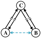
(a) A simple PCN.

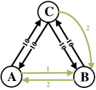
(b) The initial state.

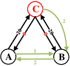
(c) A deadlock at C.

Figure 1: Examples illustrating the PCNs.

II-B Deadlock States in PCNs

To illustrate a localized deadlock state in a PCN, we consider the initial scenario depicted in Fig. 1(b). In this setup, $A$ and $C$ transfer funds to $B$ at rates of one and two tokens per second, respectively, while $B$ transfers to $A$ at a rate of two tokens per second. Notably, the specified payment rates are unbalanced, resulting in a net outflow of funds from $C$ to $A$ and $B$. Initially, each payment channel maintains a balance of ten tokens in both directions. Assuming transactions occur solely between $A$ and $B$, the system’s total throughput can only achieve two tokens per second if $A$ and $B$ transfer funds to each other at a rate of one token per second. However, after executing payments according to the initial settings, the system’s throughput gradually declines to zero. As $C$ transfers funds to $B$ faster than $A$ replenishes $C$, $C$ exhausts its funds for transfers, as illustrated in Fig. 1(c). Nonetheless, $C$ requires positive funding to route transactions between $A$ and $B$. Even if sufficient funds exist between $A$ and $B$, transactions cannot occur, leading to a network deadlock.

II-C Trusted Execution Environment

Splicer⁺ implements the security properties with Intel SGX, the most popular TEE technique, which can be used to create a protected and isolated execution environment called the enclave. SGX guarantees the confidentiality and integrity of off-chain PCHs routing computation and provides proof/attestation of the execution correctness for a particular program through remote attestation. Intel Attestation Service (IAS) serves as a trusted third-party service to verify the validity of the above correctness proof.

Remote attestation verifies the secure execution of specific code within the enclave by a digital signature of both the program and its execution output with the processor’s hardware private key. Moreover, during remote attestation, the remote client commonly employs the Diffie-Hellman key exchange protocol to negotiate a session key, enabling the establishment of a secure communication channel with the enclave to uphold communication confidentiality [24].

III Splicer⁺: Problem Statement

In this section, we outline the system model, topology, and workflow of Splicer⁺, illustrate the trust, communication, and threat models, and sketch the placement and routing problems.

III-A System Model

In Splicer⁺, two types of entities exist:

• Client. End-users in a PCN capable of sending or receiving payments. These users are typically lightweight and suitable for mobile or Internet of Things (IoT) devices. They delegate payment routing computation to smooth nodes and interact with a designated smooth node.

• Smooth node. Entities within the network responsible for processing client payment requests and executing routing protocols within their enclaves. Smooth nodes support TEE and possess adequate funds. They determine routing paths for their directly connected clients’ current payment requests and produce attestations validating payment execution correctness. Moreover, multiple smooth nodes collectively form a key management group (KMG) that manages keys using a distributed key generation protocol [26].

PCN topology with PCHs. Fig. 2(a) illustrates the star-like PCN topology in advanced PCH schemes, where a PCH establishes payment channels with multiple clients. Consequently, clients must route payments through an intermediate PCH for one-hop routing. In Splicer⁺, we depict PCNs using a multi-star-like topology, with clients uniformly connected to PCHs. Fig. 2(b) presents an example with $N$ senders and $M$ receivers among the clients, and the smooth nodes include $Z$ PCHs. We define the multi-star-like PCN topology as follows.

Definition 1.

(Multi-star-like PCN topology). In a multi-star-like PCN topology, multiple PCHs are directly or indirectly connected. Each client conducts transfers through the PCH to which it is directly connected.

It is worth noting that the payment hub model has been widely adopted in PCNs (e.g., [6, 7, 17, 16]). However, we are the first to propose a multi-star-like PCN with multiple PCHs.

(a) Star-like topology.

(b) Multi-star-like topology.

Figure 2: PCHs topologies.

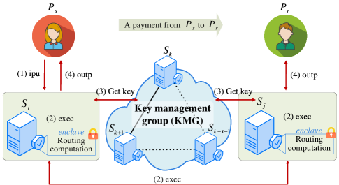
Figure 3: Workflow in multi-hop working model.

Workflow. A PCN can be represented as a graph $\mathbb{G}=(\mathbb{V},\mathbb{E})$, where $\mathbb{V}$ denotes the set of nodes and $\mathbb{E}$ denotes the set of payment channels between them. $\mathbb{V}_{\rm CLI}\subseteq\mathbb{V}$ refers to the clients, while $\mathbb{V}_{\rm SN}\subseteq\mathbb{V}$ represents the smooth nodes, with $\mathbb{V}_{\rm CLI}=\mathbb{V}-\mathbb{V}_{\rm SN}$. As illustrated in Fig. 3, when a payment occurs from client $P_{s}$ to client $P_{r}$, $S_{i}$ and $S_{j}$ denote the smooth nodes they are connected to, with $P_{s},P_{r}\in\mathbb{V}_{\rm CLI}$ and $S_{i},S_{j}\in\mathbb{V}_{\rm SN}$. The KMG comprises $\iota$ smooth nodes, where $\iota$ is a system parameter. We now outline the payment workflow, encompassing three main stages: initialization, processing, and acknowledgment by the clients/smooth nodes.

a) Payment preparation: For simplicity, we omit the detailed process of creating payment channels, and the channels’ initial deposits are assumed to be sufficient, following similar practices as described in Ref. [27, 28]. Subsequently, $P_{s}$ establishes a secure communication channel with $S_{i}$’s enclave via remote attestation, as does $P_{r}$ with $S_{j}$. Following this, payment channels are established between $P_{s}$ and $S_{i}$, as well as between $P_{r}$ and $S_{j}$. $P_{s}$ then initiates a payment request $\textsf{pay}_{\rm{req}}$ to $S_{i}$ via the secure communication channel, signaling to $S_{i}$ the initiation of a new transaction. Consequently, $S_{i}$ commences the payment initialization process. Initially, $S_{i}$ generates a fresh transaction ID tid and acquires a new key pair ($\textsf{pk}_{{\color[rgb]{0,0,0}\textsf{tid}}}$, $\textsf{sk}_{{\color[rgb]{0,0,0}\textsf{tid}}}$) from the KMG. $S_{i}$ then transmits tid and the corresponding public key $\textsf{pk}_{{\color[rgb]{0,0,0}\textsf{tid}}}$ to $P_{s}$, while retaining $\textsf{sk}_{{\color[rgb]{0,0,0}\textsf{tid}}}$ within its enclave. Subsequently, $S_{i}$ generates the initial state $\textsf{state}_{{\color[rgb]{0,0,0}\textsf{tid}}}=({\color[rgb]{0,0,0}\textsf{tid}},\theta_{{\color[rgb]{0,0,0}\textsf{tid}}})$, comprising tid and a boolean $\theta_{{\color[rgb]{0,0,0}\textsf{tid}}}$ indicating the completion status of the transaction.

b) Payment execution: The steps of payment execution are depicted in Fig. 3 as follows:

(1) The processing of a transaction tid involves generating an encrypted input inp containing the payment demand $D_{{\color[rgb]{0,0,0}\textsf{tid}}}$. Here, $D_{{\color[rgb]{0,0,0}\textsf{tid}}}=(P_{s},P_{r},\textsf{val}_{{\color[rgb]{0,0,0}\textsf{tid}}})$ denotes the payment demand of $P_{s}$, where $\textsf{val}_{{\color[rgb]{0,0,0}\textsf{tid}}}$ represents the payment amount. Initially, $P_{s}$ computes $\textsf{inp}=\textsf{Enc}(\textsf{pk}_{{\color[rgb]{0,0,0}\textsf{tid}}},D_{{\color[rgb]{0,0,0}\textsf{tid}}})$ and then sends a message $({\color[rgb]{0,0,0}\textsf{tid}},\textsf{inp})$ along with the payment funds to $S_{i}$.

(2-3) $S_{i}$ loads inp into the enclave and decrypts it with $\textsf{sk}_{{\color[rgb]{0,0,0}\textsf{tid}}}$ to obtain $D_{{\color[rgb]{0,0,0}\textsf{tid}}}=\textsf{Dec}(\textsf{sk}_{{\color[rgb]{0,0,0}\textsf{tid}}},\textsf{inp})$. Subsequently, the payment routing process commences. Within the enclave, the routing program prog divides $D_{{\color[rgb]{0,0,0}\textsf{tid}}}$ into $K$ transaction-units (TUs) $D_{{\color[rgb]{0,0,0}\textsf{tuid}}}$, each assigned a fresh ID tuid. For each $D_{{\color[rgb]{0,0,0}\textsf{tuid}}}$, $S_{i}$ generates a corresponding state $\textsf{state}_{{\color[rgb]{0,0,0}\textsf{tuid}}}^{i}=({\color[rgb]{0,0,0}\textsf{tuid}},\theta_{{\color[rgb]{0,0,0}\textsf{tuid}}}^{i})$, where $\theta_{{\color[rgb]{0,0,0}\textsf{tuid}}}^{i}$ indicates the completion status of the transaction-unit, and $\theta_{{\color[rgb]{0,0,0}\textsf{tid}}}=\bigwedge_{1\leq i\leq K}\theta_{{\color[rgb]{0,0,0}\textsf{tuid}}}^{i}$. $S_{j}$ acquires the ($\textsf{pk}_{{\color[rgb]{0,0,0}\textsf{tuid}}},\textsf{sk}_{{\color[rgb]{0,0,0}\textsf{tuid}}}$) pair from the KMG. $S_{i}$ then encrypts $D_{{\color[rgb]{0,0,0}\textsf{tuid}}}$ using $\textsf{pk}_{{\color[rgb]{0,0,0}\textsf{tuid}}}$ and sends it to $S_{j}$, who decrypts it using $\textsf{sk}_{{\color[rgb]{0,0,0}\textsf{tuid}}}$. Upon receiving the corresponding funds, $S_{j}$ sends a payment acknowledgment $\textsf{ACK}_{{\color[rgb]{0,0,0}\textsf{tuid}}}$ to $S_{i}$ via a secure communication channel, prompting $S_{i}$ to update $\textsf{state}_{{\color[rgb]{0,0,0}\textsf{tuid}}}^{i}$ to indicate transaction completion. After receiving all acknowledgments $\textsf{ACK}_{{\color[rgb]{0,0,0}\textsf{tuid}}}$, $S_{i}$ updates $\textsf{state}_{{\color[rgb]{0,0,0}\textsf{tid}}}$ and generates an attestation/proof $\sigma_{{\color[rgb]{0,0,0}\textsf{tid}}}=\Sigma.\textsf{Sig}(\textsf{msk},(\textsf{prog},\textsf{state}_{{\color[rgb]{0,0,0}\textsf{tid}}}))$ using a digital signature scheme $\Sigma$ and the manufacturer-generated processor private key msk of $S_{i}$. $\sigma_{{\color[rgb]{0,0,0}\textsf{tid}}}$ verifies the correctness of the payment routing program execution.

(4) Eventually, $S_{j}$ receives all TUs of $D_{{\color[rgb]{0,0,0}\textsf{tid}}}$ and transfers the payment funds to $P_{r}$ in a single transaction. $P_{r}$ then produces a successful receipt acknowledgment $\textsf{ACK}_{{\color[rgb]{0,0,0}\textsf{tid}}}$, which is ultimately relayed to $P_{s}$ by the smooth nodes.

Additionally, after a payment, any party can verify the authenticity of the attestation $\sigma_{{\color[rgb]{0,0,0}\textsf{tid}}}$ by sending it to the IAS. It generates a proof $\pi_{{\color[rgb]{0,0,0}\textsf{tid}}}=(b,\sigma_{{\color[rgb]{0,0,0}\textsf{tid}}},\sigma_{\textsf{IAS}})$, where $b\in\{0,1\}$ denotes the validity of $\sigma_{{\color[rgb]{0,0,0}\textsf{tid}}}$, and $\sigma_{\textsf{IAS}}$ is a signature over $b$ and $\sigma_{{\color[rgb]{0,0,0}\textsf{tid}}}$ by IAS. Moreover, in the outlined workflow, any payment sender is required to pay an extra forwarding fee to the intermediaries along the routing path, serving as an incentive for smooth nodes, as detailed in §IV-D.

III-B Trust, Communication, and Threat Models

Trust model. Splicer⁺ operates as a community-autonomous system, facilitating a certain level of trust transfer among entities. As illustrated in Fig. 4, Splicer⁺ employs a multiwinner voting algorithm (e.g., [29, 30]) within the smart contract, enabling all entities to impartially select a smooth node candidate list over an extended period. This algorithm considers two key properties: (i) Excellence, indicating that selected candidates are more suitable for outsourcing routing tasks (e.g., possessing more client connections, transaction funds, and lower operational overhead), and (ii) Diversity, aiming for a diverse distribution of candidate positions. As the optimal design of multiwinner voting is not the primary focus of this paper, it is deferred to future research.

Initially, the first selected candidate smooth nodes serve temporarily in payment routing, acting as actual PCHs. Once the network state stabilizes, the candidate smooth nodes execute a smart contract containing a placement optimization algorithm to ascertain the actual PCHs (long-term operation). It is noteworthy that once the distribution of transaction requests stabilizes within the network, the overall request distribution information acquired by each candidate PCH aligns, leading to the consistent determination of actual PCHs.

Fig. 4 illustrates that this process removes redundant payment channels, thereby simplifying the network’s complexity. Actual PCHs are required to pledge funds to a public pool for access, and their behavior is mutually checked and balanced; any malicious or colluding PCHs will be identified by others. Additionally, Splicer⁺ offers clients a reporting and arbitration mechanism. Malicious PCHs will be expelled, and their deposits confiscated as punishment (where the loss outweighs the profit). Subsequently, new PCHs will be selected from the updated candidate list to fill the vacancies, discouraging rational PCHs from engaging in corruption. It is worth emphasizing that sensitive information (e.g., node identities, transaction values, routing data) is transmitted in ciphertext and computed confidentially within the TEE, alleviating client concerns regarding privacy breaches.

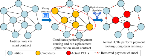
Figure 4: System trust transference model.

Communication model. Illustrated in Fig. 5, we outline the communication process. Splicer⁺ operates within a bounded synchronous communication framework. At the start of epoch $e$+1, PCHs acquire and synchronize the conclusive global information from the previous epoch, encompassing clients’ statuses and network data (e.g., topology, channel conditions, payment flow rate). Concurrently, upon receipt of local payment requests from directly connected clients, each PCH formulates decentralized routing decisions relying on the network data (final global information of epoch $e$) and the recent requests from its clients (local information of epoch $e$+1). Subsequently, recipients generate payment acknowledgments, which PCHs transmit to senders. Splicer⁺ iterates through this process continuously.

Figure 5: System communication process in epoch $e$+1.

Threat model. Each PCH is rational and potentially malicious, willing to deviate from the protocol to gain advantages. An adversary could compromise a target PCH’s operating system and network stack, allowing arbitrary dropping, delaying, and replaying of messages. As the adversary would not benefit from corrupting the PCH placement process, their attack might only result in the failure of payment routing for some transactions. Nevertheless, the failed transactions will be rolled back by the PCH, causing no losses to the client or system stability.

Assume all entities trust Intel’s processor and its attestation keys. Entities cannot feasibly generate any correctness proof of program execution, except through SGX remote attestation, making the proofs existentially unforgeable. Each client trusts the PCH’s enclave after remote attestation and the program execution proof verified by the IAS.

We acknowledge that current TEE instances are vulnerable to side-channel attacks [31, 32]. Splicer⁺ employs a cryptographic library resistant to side-channel attacks to mitigate this vulnerability. We emphasize that addressing side-channel attack resistance is not the primary focus of this work, as it is of independent interest.

III-C PCH Placement and Routing Problems

Placement problem. The essence of the placement problem lies in selecting the actual PCHs from the smooth node candidate list and deploying them to execute the PCH program for payment routing, facilitated by a fixed, long-running placement optimization smart contract. The placement optimization smart contract determines the quantity and positions of the actual PCHs within the network. It is important to note that this process is community-driven and decentralized, rather than centrally controlled. During long-term stable operation, the selection of actual PCHs remains unchanged unless the network deviates from its optimal operational state (resulting in changes to the output of the placement optimization smart contract) or a malicious PCH is identified and removed. In practice, the community evaluates the costs and benefits to decide when it is necessary to address a new placement problem.

Due to the presence of numerous geographically dispersed nodes in real PCNs, PCHs may be distant from certain clients, resulting in unstable connections or high communication delays and overheads. Our objective is to evenly position the PCHs close to the clients, ensuring that all clients have the fewest average payment hops required for routing. While physically dispersed, PCHs are logically polycentric and collaborate in managing payment routing. This placement strategy reduces the distance between nodes, while also taking into account the expenses associated with PCHs collecting client statistics and synchronizing among themselves. It results in a network load tradeoff: (i) PCHs should be proximate to their routed clients to minimize communication delay and route management overhead (management cost); (ii) they should be close to each other to minimize the delay and overhead associated with synchronizing states (synchronization cost). Therefore, the appropriate placement of PCHs in a PCN poses a placement problem. We are the first to address the PCH placement problem in PCNs, and further elaborate on the specifics of this problem in §IV-B, along with proposed solutions in §IV-C.

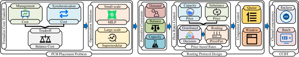
Figure 6: The overall structure of our design.

Routing problem. Existing routing solutions aim to: (i) minimize routing costs to enhance throughput, and (ii) redistribute channel funds to improve routing performance. However, source routing requires each sender to compute routing paths, which is impractical in large-scale scenarios (Until March 12, 2024, the total number of nodes in the Lightning Network is 14,023. This paper considers a network with over 3,000 nodes as large-scale). A distributed routing decision protocol across multiple PCHs needs to be designed. Thus, we propose a rate-based routing mechanism inspired by packet-switching technique. Transactions are divided into multiple independently routed TUs by each PCH. Each TU can transfer a specified amount of funds within Min-TU and Max-TU constraints at varying rates. We emphasize that this multi-path payment routing approach has been successfully demonstrated in Spider [12]. It does not compromise payment confidentiality as each TU is encrypted with a unique public key from the KMG. Furthermore, different intermediate nodes may be involved in each TU routing path, complicating the relationship between parties in multiple original transactions within PCNs. Therefore, Splicer⁺ inherits the unlinkability of advanced PCHs (the proof of unlinkability is omitted). Coupled with TEE’s confidential routing computation, intermediaries face increased difficulty in recognizing ciphertexts containing sensitive information. Further details of our routing protocol are provided in §IV-D.

IV System Design

IV-A Overview

The structure of our design is illustrated in Fig. 6. Initially, we address the placement of smooth nodes. The placement problem involves balancing routing management and synchronization costs. We now delve into the specifics of the smooth nodes placement problem, framing it as an optimization challenge with dual cost considerations and aiming to minimize the balance cost. Subsequently, we offer solutions for the transformed optimization problem at two scales of PCN. For small-scale networks, we convert the placement problem into a mixed-integer linear programming (MILP) problem to determine the optimal solution. Supermodular function techniques are employed to approximate the solution in a large-scale network.

Subsequently, we delve into the specifics of routing protocol design for smooth nodes. Initially, we outline the formal constraints of the routing problem, encompassing demand, capacity, and balance constraints. We then address transaction flow rate control based on routing price. We define the capacity and imbalance prices, calculate the routing price and fee through distributed decisions, and determine the flow rates based on pricing. Finally, we address congestion control during routing and design the waiting queue and window to mitigate congestion.

Ultimately, leveraging TEE-enabled PCHs grants Splicer⁺ a new capability: facilitating the establishment of concurrent payment channels between smooth nodes. We introduce the channel concurrency benefit theory (CCBT) to analyze the correlation between channel concurrency and throughput benefits. Additionally, we implement batch processing of transactions on smooth nodes.

IV-B Formalize the Placement Problem

We elaborate on the long-term periodic election of the smooth node candidate list in the trust model outlined in §III-B. We provide a succinct overview of the PCH placement problem in §III-C. Subsequently, we delve deeper into modeling the selection of actual PCHs from the candidate list.

For a formal depiction of the network load tradeoff, we define two binary variables $x_{n},y_{mn}\in\left\{0,1\right\}$ representing whether a candidate node $n\in\mathbb{V}_{\rm SNC}$ (where $\mathbb{V}_{\rm SNC}$ denotes the set of candidate smooth nodes) can act as a smooth node and whether a client $m\in\mathbb{V}_{\rm CLI}$ is directly connected to a smooth node $n$, respectively. Thus, the vectors $\bm{x}$ and $\bm{y}$ represent the placement and assignment strategies, respectively:

$$\bm{x}=(x_{n}\in\left\{0,1\right\}:n\in\mathbb{V}_{\rm SNC}),$$ (1)

$$\bm{y}=(y_{mn}\in\left\{0,1\right\}:m\in\mathbb{V}_{\rm CLI},\,n\in\mathbb{V}_{\rm SNC}).$$ (2)

A node $n$ that is not suitable for placement as a smooth node ($x_{n}=0,\forall n\notin\mathbb{V}_{\rm SNC}$). Each client must be assigned to a smooth node, necessitating $\sum_{n\in\mathbb{V}_{\rm SNC}}y_{mn}=1,\forall m\in\mathbb{V}_{\rm CLI}$. To enable the assignment of client $m$, node $n$ must be designated as a smooth node ($y_{mn}\leq x_{n},\forall m\in\mathbb{V}_{\rm CLI},n\in\mathbb{V}_{\rm SNC}$).

Let $\zeta_{mn}$ and $\delta_{nl}$ represent the management cost of assigning a client $m\in\mathbb{V}_{\rm CLI}$ to a smooth node $n\in\mathbb{V}_{\rm SNC}$ and the synchronization cost between two smooth nodes $n,l\in\mathbb{V}_{\rm SNC}$, respectively. Notably, $\zeta_{mn}$ and $\delta_{nl}$ are local or edge-wise parameters probed by candidate smooth nodes during the last long period. Subsequently, the total management cost and synchronization cost in the network can be formulated as

$$\mathcal{C}_{M}(\bm{y})=\sum_{m\in\mathbb{V}_{\rm CLI}}\sum_{n\in\mathbb{V}_{\rm SNC}}\zeta_{mn}y_{mn},$$ (3)

$$\mathcal{C}_{S}(\bm{x},\bm{y})=\sum_{n\in\mathbb{V}_{\rm SNC}}\sum_{l\in\mathbb{V}_{\rm SNC}}x_{n}x_{l}(\delta_{nl}\sum_{m\in\mathbb{V}_{\rm CLI}}y_{mn}+\epsilon_{nl}).$$ (4)

Here, $\epsilon_{nl}$ represents the constant cost in synchronization.

The tradeoff is redefined as a balance between the costs presented in equations (3)-(4). Let $\omega\geq 0$ represent the weighting factor between the two costs, and the balanced cost can be expressed as

$$\mathcal{C}_{B}(\bm{x},\bm{y})=\mathcal{C}_{M}(\bm{y})+\omega\mathcal{C}_{S}(\bm{x},\bm{y}).$$ (5)

The PCH placement problem is formulated as $\min\mathcal{C}_{B}(\bm{x},\bm{y})$, with constraints represented by formulas (1)-(2). This problem is intricate due to the presence of discrete variables and a nonlinear objective function (4) comprising cubic and quadratic terms, rendering it a classical NP-hard problem [33].

IV-C Optimization Placement Problem Solutions

Small-scale optimal solution. We transform the placement problem into a MILP problem to obtain the optimal solution for small-scale scenarios. This conversion is crucial as it simplifies the problem into one with a linear objective function and constraints, making it readily solvable by various commercial solvers.

We employ standard linearization techniques to facilitate this conversion process. Initially, we introduce two vectors, $\bm{\vartheta}$ and $\bm{\varphi}$, as additional optimization variables.

$$\bm{\vartheta}=(\vartheta_{nl}\in\left\{0,1\right\}:n,l\in\mathbb{V}_{\rm SNC}),$$ (6)

$$\bm{\varphi}=(\varphi_{nlm}\in\left\{0,1\right\}:n,l\in\mathbb{V}_{\rm SNC},\,m\in\mathbb{V}_{\rm CLI}).$$ (7)

Second, the linear constraints for $\vartheta$ and $\varphi$ are defined as follows:

$$\vartheta_{nl}\leq x_{n},\quad\vartheta_{nl}\leq x_{l},\quad\vartheta_{nl}\geq x_{n}+x_{l}-1,\quad n,l\in\mathbb{V}_{\rm SNC},$$ (8)

$$\begin{split}\varphi_{nlm}\leq\vartheta_{nl},\quad\varphi_{nlm}\leq y_{mn},\quad\varphi_{nlm}\geq\vartheta_{nl}+y_{mn}-1,\\ \quad n,l\in\mathbb{V}_{\rm SNC},\,m\in\mathbb{V}_{\rm CLI}.\end{split}$$ (9)

The constraints in (8) imply that if either $x_{n}$ or $x_{l}$ is 0, $\vartheta_{nl}$ must be 0; otherwise, it is set to 1. Similarly, the constraints in (9) follow the same principle.

Third, we linearize the cost function (4) using the new variables, resulting in

$$\widehat{\mathcal{C}}_{S}(\bm{\vartheta},\bm{\varphi})=\sum_{n\in\mathbb{V}_{\rm SNC}}\sum_{l\in\mathbb{V}_{\rm SNC}}(\sum_{m\in\mathbb{V}_{\rm CLI}}\delta_{nl}\varphi_{nlm}+\epsilon_{nl}\vartheta_{nl}).$$ (10)

Finally, the MILP problem can be formulated as $\min\mathcal{C}_{M}(\bm{y})+\omega\widehat{\mathcal{C}}_{S}(\bm{\vartheta},\bm{\varphi})$, subject to the constraints defined by formulas (1)-(2) and (8)-(9).

Thus, the conversion of the PCH placement problem to a MILP problem enables direct solutions using existing commercial solvers. Typically, these solvers employ a combination of the branch and bound method and the cutting-plane method, enabling fast resolution of the MILP problem for small-scale scenarios. However, since our model encompasses payments involving mobile or IoT devices, and the scale of PCNs can be immense, this results in an exceedingly large MILP problem, posing computational challenges for solvers. To address this, we propose an approximate solution for tackling large-scale problems.

Large-scale approximation solution. Firstly, we introduce a lemma that elucidates the relationship between the placement plan $\bm{x}$ and the assignment plan $\bm{y}$.

Lemma 1.

Given a placement plan $\bm{x}$, for each $m\in\mathbb{V}_{\rm CLI},n\in\mathbb{V}_{\rm SNC}$, the optimal assignment plan $\bm{y}$ can be expressed as

$$\hskip-5.69054pty_{mn}=\left\{\begin{aligned} &1,\,\,if\,\,n=\mathop{\arg\min}_{n^{\prime}\in\mathbb{V}_{\rm SNC}:x_{n^{\prime}}=1}(\omega\sum_{l\in\mathbb{V}_{\rm SNC}:x_{l}=1}\delta_{n^{\prime}l}+\zeta_{mn^{\prime}}),\\ &0,\,\,otherwise.\end{aligned}\right.$$ (11)

Proof.

Assuming there exists an optimal assignment plan $\bm{y^{o}}$, in which client $m^{o}$ is assigned to smooth node $n^{o}$. Then there exists another node $n^{h}\neq n^{o}$ and $n^{h}=1$, let

$$\omega\sum_{l\in\mathbb{V}_{\rm SNC}:x_{l}=1}\delta_{n^{h}l}+\zeta_{mn^{h}}<\omega\sum_{l\in\mathbb{V}_{\rm SNC}:x_{l}=1}\delta_{n^{o}l}+\zeta_{mn^{o}}.$$ (12)

This indicates that if client $m^{o}$ is reassigned to smooth node $n^{h}$, the management cost decreases by $\zeta_{mn^{o}}-\zeta_{mn^{h}}$, and the synchronization cost decreases by $\sum_{l\in\mathbb{V}_{\rm SNC}:x_{l}=1}\delta_{n^{o}l}-\sum_{l\in\mathbb{V}_{\rm SNC}:x_{l}=1}\delta_{n^{h}l}$. Consequently, the objective function $\mathcal{C}_{B}$ decreases by $\omega\sum_{l\in\mathbb{V}_{\rm SNC}:x_{l}=1}\delta_{n^{o}l}+\zeta_{mn^{o}}-\omega\sum_{l\in\mathbb{V}_{\rm SNC}:x_{l}=1}\delta_{n^{o}l}-\zeta_{mn^{o}}>0$. However, this contradicts our assumption that $\bm{y^{o}}$ is an optimal assignment plan.∎

Lemma 1 suggests that finding the assignment plan $\bm{y}$ for a given placement plan $\bm{x}$ is straightforward. Thus, our focus is on optimizing the placement plan. Let $X_{n}$ represent the placement of smooth node $n$ (i.e., $x_{n}=1$), and the set of all possible placements of smooth nodes is denoted by

$$\mathcal{S}=(X_{n}:n\in\mathbb{V}_{\rm SNC}).$$ (13)

This implies that if and only if $X_{n}\in\mathcal{X}$, where $\mathcal{X}\subseteq\mathcal{S}$, a subset $\mathcal{X}$ represents a placement plan $\bm{x}$ such that $x_{n}=1$. Let $\bm{x}_{\mathcal{X}}$ denote the binary representation of $\mathcal{X}$, then the balance cost objective function $\mathcal{C}_{B}$ can be represented as a set function $f:2^{\mathcal{S}}\rightarrow\mathbb{R}$

$$f(\mathcal{X})=\mathcal{C}_{B}(\bm{x}_{\mathcal{X}},y(\bm{x}_{\mathcal{X}})).$$ (14)

Here, $y(\bm{x}_{\mathcal{X}})$ denotes the optimal assignment plan given the smooth node placement plan $\bm{x}_{\mathcal{X}}$ according to equation (11).

Secondly, we consider a well-studied class of set functions known as supermodular functions [34].

Definition 2.

A set function $f:2^{\mathcal{S}}\rightarrow\mathbb{R}$ defined on a finite set $\mathcal{S}$ is termed supermodular if for all subsets $\mathcal{A},\mathcal{B}\subseteq\mathcal{S}$ with $\mathcal{A}\subseteq\mathcal{B}$ and every element $i\in\mathcal{S}\setminus\mathcal{B}$, the following condition holds:

$$f(\mathcal{A}\cup\left\{i\right\})-f(\mathcal{A})\leq f(\mathcal{B}\cup\left\{i\right\})-f(\mathcal{B}),$$ (15)

This condition indicates that when an element $i$ is added to a set, the marginal value increases as the set expands.

Lemma 2.

The set function $f(\mathcal{X})$ is supermodular in the case of uniform costs $\delta_{nl}=\delta_{n^{\prime}l^{\prime}}=\delta$, $\forall n,l,n^{\prime},l^{\prime}\in\mathbb{V}_{\rm SNC}$.

Lemma 2 has been proven in [33]. Building upon this, the placement problem can be formulated as the minimization of a supermodular function $f$.

Input: Two initially solutions $X_{0}^{s}$, $Y_{0}^{s}$, element $u_{i}$

Output: Final solution $X_{z}^{s}$ (or equivalently $Y_{z}^{s}$)

1 for $i=1$ to $z$ do

    // Maintain the two solutions until they coincide

2    $a_{i}\leftarrow f(X_{i-1}^{s}\cup\left\{u_{i}\right\})-f(X_{i-1}^{s})$

3    $b_{i}\leftarrow f(Y_{i-1}^{s}\setminus\left\{u_{i}\right\})-f(Y_{i-1}^{s})$

4    $a_{i}^{\prime}\leftarrow\max\left\{a_{i},0\right\}$, $b_{i}^{\prime}\leftarrow\max\left\{b_{i},0\right\}$

5    if $a_{i}^{\prime}/(a_{i}^{\prime}+b_{i}^{\prime})^{\star}$ then

6       $X_{i}^{s}\leftarrow X_{i-1}^{s}\cup\left\{u_{i}\right\}$, $Y_{i}^{s}\leftarrow Y_{i-1}^{s}$

7      

8   else

9       $X_{i}^{s}\leftarrow X_{i-1}^{s}$, $Y_{i}^{s}\leftarrow Y_{i-1}^{s}\setminus\left\{u_{i}\right\}$

10      

11   

12return $X_{z}^{s}$ (or equivalently $Y_{z}^{s}$)

^⋆ If $a_{i}^{\prime}=b_{i}^{\prime}=0$, then $a_{i}^{\prime}/(a_{i}^{\prime}+b_{i}^{\prime})=1$

Algorithm 1 Placement Approximation Algorithm

Thirdly, solving such problems is equivalent to dealing with their maximization versions of submodular functions. Let $f^{ub}$ denote an upper bound on the maximum possible value of $f(\mathcal{X})$, and the submodular function is represented as $\widehat{f}(\mathcal{X})=f^{ub}-f(\mathcal{X})$.

Several approximation algorithms (e.g., [35, 36]) exist to maximize $\widehat{f}(\mathcal{X})$. An approximation bound $\psi$ specifies that the value ratio of the approximate solution to the optimal solution is always at least $\psi$. The algorithm proposed in [36] offers the most favorable approximation bound, where $\psi=\frac{1}{2}$. In Alg. 1, the algorithm iterates $z=|\mathbb{V}_{\rm SNC}|$ times, with $u_{i}(1\leq i\leq z)$ representing an arbitrary element from set $\mathcal{S}$. Initially, two solutions $X^{s}$ and $Y^{s}$ are set as $X_{0}^{s}\leftarrow\varnothing$ and $Y_{0}^{s}\leftarrow\mathcal{S}$. Lines 1-1 operate as follows: At the $i^{th}$ iteration, the algorithm randomly and greedily adds $u_{i}$ to $X_{i-1}^{s}$ or removes $u_{i}$ from $Y_{i-1}^{s}$ based on the marginal gain of each option. After $z$ iterations, both solutions converge (i.e., $X_{z}^{s}=Y_{z}^{s}$), and this is returned at line 1. Line 1 addresses a special case from line 1 where $a_{i}^{\prime}=b_{i}^{\prime}=0$. Finally, based on the aforementioned steps, we obtain an approximate solution for large-scale network instances.

IV-D Rate-Based Routing Protocol Design

Formal constraints. For a given path $p$, $r_{p}$ denotes the payment rate from its source to its destination. We assume TUs traverse a payment channel with capacity $c_{a,b}$ from smooth node $a$ to another smooth node $b$ at rate $r_{a,b}$.Upon payment forwarding, an average time $\Delta$ is required to receive acknowledgment of the TUs from the destination, resulting in $r_{a,b}\Delta$ funds being locked in the channel. The capacity constraint ensures that the average rate on the channel does not surpass $c_{a,b}/\Delta$. Additionally, a balance constraint mandates that the one-directional payment rate $r_{a,b}$ aligns with the rate $r_{b,a}$ in the opposite direction to maintain channel fund equilibrium. Otherwise, funds gravitate toward one end of the channel, potentially leading to a local deadlock where all funds converge at one end (see §II-B).

To ensure optimal fund utilization within channels, we adopt a widely used utility model for payment transactions. This model assigns utility to each source based on the logarithm of the total rate of outgoing payments [37]. Thus, our objective is to maximize the overall utility across all source-destination pairs, while adhering to the aforementioned constraints:

$$\max\quad \sum_{s,e\in\mathbb{V}}log(\sum_{p\in\mathbb{P}_{s,e}}r_{p})$$ (16)

$$s.t.\quad \sum_{p\in\mathbb{P}_{s,e}}r_{p}\Delta\leq d_{s,e}\quad\ \forall s,e\in\mathbb{V}$$ (17)

$$\ r_{a,b}+r_{b,a}\leq\frac{c_{a,b}}{\Delta}\quad\forall(a,b)\in\mathbb{E}$$ (18)

$$\ \lvert r_{a,b}-r_{b,a}\rvert\leq\epsilon\ \ \ \ \,\,\forall(a,b)\in\mathbb{E}$$ (19)

$$\ r_{p}\geq 0\qquad\qquad\ \ \ \ \,\forall p\in\mathbb{P},$$ (20)

where $s$ is the starting point and $e$ represents the endpoint. $\mathbb{P}_{s,e}$ denotes the set of all paths from $s$ to $e$, and $d_{s,e}$ indicates the demand from $s$ to $e$. $c_{a,b}$ represents the capacity of the channel $(a,b)$, while $\mathbb{P}$ represents the set of all paths. Formula (17) represents the demand constraint, ensuring that the total flow across all paths does not exceed the total demand. Formula (18) and (19) represent the capacity and balance constraints, respectively. The balance constraint may be stringent in the ideal scenario (i.e., when the system parameter $\epsilon=0$), but we aim for the flow rates in both channel directions to approach equilibrium in practice (i.e., when $\epsilon$ is sufficiently small).

Distributed routing decisions. Each PCH makes distributed routing decisions for payments based on the network data of the last epoch and its clients’ requests in the current epoch. Utilizing primal-dual decomposition techniques [38], we address the optimization problem for a generic utility function $U(\sum_{p\in\mathbb{P}_{s,e}}r_{p})$. Lagrangian decomposition naturally separates this linear programming problem into distinct subproblems [39]. A solution involves computing the flow rates to be maintained on each path. We establish the routing price in both directions of each channel, with PCHs adjusting the prices to regulate the flow rates of TUs. Additionally, the routing price serves as the forwarding fee to incentivize PCHs.

The routing protocol is depicted in Alg. 2. (Lines 2-2) The payment demand $D_{s,e}$ is decrypted, and the smooth node divides it into $k$ packets of TUs $d_{i}$. We constrain $\textit{Min-TU}\leq|d_{i}|\leq\textit{Max-TU}$ to control the number of split TUs, where $|D_{s,e}|=\sum_{i=1}^{k}|d_{i}|$. There are $k$ paths $\{p_{i}\}_{1\leq i\leq k}\in\mathbb{P}_{s,e}$ (refer to §VI-D for a discussion on path selection). For conciseness, we only examine a channel $(a,b)$ in path $p_{i}$, denoted as $(a,b)\in p_{i}$. Here, $\lambda_{a,b}$ denotes the capacity price, indicating when the total transaction rate exceeds the capacity. Additionally, $\mu_{a,b}$ and $\mu_{b,a}$ represent the imbalance price, reflecting the disparity in rates between the two directions. These three prices are updated every $\tau$ seconds to maintain compliance with capacity and balance constraints. $n_{a}$ and $n_{b}$ denote the funds required to sustain flow rates at nodes $a$ and $b$, respectively. The capacity price $\lambda_{a,b}$ is updated as:

$$\lambda_{a,b}(t+1)=\lambda_{a,b}(t)+\kappa(n_{a}(t)+n_{b}(t)-c_{a,b}),$$ (21)

where $\kappa$ is a system parameter utilized to regulate the rate of price adjustment. If the required funds exceed the capacity $c_{a,b}$, the capacity price $\lambda_{a,b}$ increases, indicating the necessity to decrease the rates via $(a,b)$, and vice-versa.

Let $m_{a}$ and $m_{b}$ denote the TUs that arrived at $a$ and $b$ in the previous period, respectively. The imbalance price $\mu_{b,a}$ is updated as:

$$\mu_{a,b}(t+1)=\mu_{a,b}(t)+\eta(m_{a}(t)-m_{b}(t)).$$ (22)

Here, $\eta$ represents a system parameter. If the funds flowing in the $a$ $\rightarrow$ $b$ direction exceed those in the $b$ $\rightarrow$ $a$ direction, the imbalance price $\mu_{a,b}$ increases while $\mu_{b,a}$ decreases. This adjustment prompts a reduction in the flow rates along the $(a,b)$ route and an increase along the $(b,a)$ route, ensuring a balance in the system.

Smooth nodes employ a multi-path routing protocol to regulate payment transfer rates based on routing prices and node feedback observations. Probes are periodically dispatched along each path [13], every $\tau$ seconds, to measure the aforementioned prices. The routing price for the channel $(a,b)$ is

$$\xi_{a,b}=2\lambda_{a,b}+\mu_{a,b}-\mu_{b,a},$$ (23)

the forwarding fee that $a$ needs to pay to $b$ is

$$\textsf{fee}_{a,b}=T_{\textsf{fee}}(2\lambda_{a,b}+\mu_{a,b}-\mu_{b,a}),$$ (24)

where $T_{\textsf{fee}}(0<T_{\textsf{fee}}<1)$ is a systematic threshold parameter.

Thus, the total routing price of a path $p$ is

$$\varrho_{p}=(1+T_{\textsf{fee}})\sum_{(a,b)\in p}\xi_{a,b}.$$ (25)

The total amount of excess and imbalance demands is indicated. Then, the smooth node sends a probe on path $p$, summing the price $\xi_{a,b}$ of each channel $(a,b)$ on $p$. Based on the routing price $\varrho_{p}$ from the most recently received probe, the rate $r_{p}$ is updated as

$$r_{p}(t+1)=r_{p}(t)+\alpha(U^{\prime}(r)-\varrho_{p}(t)),$$ (26)

where $\alpha$ is a system parameter. Thus, the sending rate on a path is adjusted reasonably according to the routing price.

Input: Decrypted demand $D_{s,e}$, rate $r_{p_{i}}$, required funds $n_{a}$, $n_{b}$, arrived TUs $m_{a}$, $m_{b}$

Output: Routing rates $r_{p_{i}}$ $(1\leq i\leq k)$

1 Split the demand $D_{s,e}$ into $d_{i}$ on path $p_{i}$ $(1\leq i\leq k)$.

2 for $i=1$ to $k$ do

3    for $\forall$ payment channel $(a,b)$ on path $p_{i}$ do

       // Update the routing rates

4       $\lambda_{a,b}\leftarrow\lambda_{a,b}+\kappa(n_{a}+n_{b}-c_{a,b})$

5       $\mu_{a,b}\leftarrow\mu_{a,b}+\eta(m_{a}-m_{b})$

6       $\xi_{a,b}\leftarrow 2\lambda_{a,b}+\mu_{a,b}-\mu_{b,a}$

       // Forwarding fee

7       $\textsf{fee}_{a,b}\leftarrow T_{\textsf{fee}}(2\lambda_{a,b}+\mu_{a,b}-\mu_{b,a})$

       // Routing price of the path $p_{i}$

8       $\varrho_{p_{i}}\leftarrow(1+T_{\textsf{fee}})\sum_{(a,b)\in p_{i}}\xi_{a,b}$

9       $r_{p_{i}}\leftarrow r_{p_{i}}+\alpha(U^{\prime}(r)-\varrho_{p_{i}})$

       // Congestion control

10       if $r_{p_{i}}>r_{a,b}^{\rm process}$ or $F_{a,b}<|d_{i}|$ then

11          $q_{a,b}^{\rm amount}\leftarrow d_{i}$

12          $t_{p_{i}}^{\rm delay}$ $\leftarrow$ Smooth nodes monitor

13          if $t_{p_{i}}^{\rm delay}>T$ then

14             $d_{i}^{*}\leftarrow d_{i}$

15            

16         if $d_{i}^{*}$ is aborted then

17             $w_{p_{i}}\leftarrow w_{p_{i}}-\beta$

18            

19         if $q_{a,b}^{\rm amount}<w_{p_{i}}$ and $d_{i}$ is transmitted then

20             $w_{p_{i}}\leftarrow w_{p_{i}}+\frac{\gamma}{\sum_{p_{i}^{\prime}\in\mathbb{P}_{s,e}}w_{p_{i}^{\prime}}}$

21            

22         

23      

24   return $r_{p_{i}}$

Algorithm 2 Distributed Routing Decision Protocol

Congestion control (Lines 2-2). This rate-based approach may lead to TU congestion. To manage this, we employ waiting queues and windows. When congestion arises, intermediate hubs in the path queue TUs, signifying a capacity or balance constraint violation. Thus, smooth nodes must utilize a congestion control protocol to identify capacity and imbalance violations and regulate queues by adjusting sending rates in channels.

The congestion controller has two fundamental properties aimed at achieving efficiency and balanced rates. Firstly, it aims to maintain a non-empty queue, indicating efficient utilization of channel capacity. Secondly, it ensures that queues are bounded, preventing the flow rate of each path from exceeding capacity or becoming imbalanced. Several congestion control algorithms [40] satisfy these properties and can be adapted for PCNs. Now, we provide a brief description of the protocol.

If the rate $r_{p_{i}}$ exceeds the upper limited rate $r_{a,b}^{\rm process}$ that the channel $(a,b)$ can process, or if the demand $|d_{i}|$ exceeds the current funds in the $a$ $\rightarrow$ $b$ direction $F_{a,b}$, then the protocol initiates congestion control measures. (i) Let $q_{a,b}^{\rm amount}$ denote the amount of TUs pending in queue $q_{a,b}$. The queuing delay $t_{p}^{\rm delay}$ on path $p$ is monitored by smooth nodes, and if it exceeds the predetermined threshold $T$, the packet $d_{i}$ is marked as $d_{i}^{*}$. Once a TU is marked, hubs do not process the packet but merely forward it. When the recipient sends back an acknowledgment with the marked field appropriately set, hubs forward it back to the sender. (ii) Based on observations of congestion in the network, smooth nodes regulate the payment rates transferred in the channels and select a set of $k$ paths to route TUs from $s$ to $e$. (iii) The window size $w_{p}$ represents the maximum number of unfinished TUs on path $p$. Smooth nodes maintain the window size for every candidate path to a destination, indirectly controlling the flow rate of TUs on the path. Smooth nodes keep track of unserved or aborted TUs on the paths. New TUs can be transmitted on path $p$ only if the total number of TUs to be processed does not exceed $w_{p}$. On a path $p$ from $s$ to $e$, the window is adjusted as:

$$w_{p}\left(t+1\right)=w_{p}\left(t\right)-\beta,$$ (27)

$$w_{p}\left(t+1\right)=w_{p}\left(t\right)+\frac{\gamma}{\sum_{p^{\prime}\in\mathbb{P}_{s,e}}w_{p^{\prime}}},$$ (28)

where equation (27) signifies that marked packets fail to complete the payment within the deadline, prompting senders to cancel the payment, and equation (28) indicates the transmission of unmarked packets. The positive constants $\beta$ and $\gamma$ represent the factors by which the window size decreases and increases, respectively.

Despite Spider [12] utilizing a similar multi-path payment model, Splicer⁺ differs primarily in three aspects: (i) Splicer⁺ accounts for forwarding costs, albeit with a fee model distinct from that of the Lightning Network in Spider. (ii) In addition to congestion control, Splicer⁺ also implements rate control to mitigate network capacity and imbalance violations. (iii) Routing computation in Splicer⁺ is delegated to TEE-based PCHs, contrasting with end-user processing. We assess the performance of this optimized Splicer⁺ against the Spider solution in §VI-B.

IV-E Channel Concurrency

Concurrent channels. In previous studies [4, 5], the locking of intermediate channels by multi-hop payments hindered the concurrent utilization of payment channels. Due to Splicer⁺ storing the private key controlling fund payments within the enclave, it can dynamically deposit or withdraw channel funds without blockchain access, enabling the creation of concurrent channels among compatible nodes (similar to Ref. [20]). Splicer⁺ can establish new concurrent payment channels across multiple PCHs promptly, using unassociated deposits aligned with PCHs’ payment routing needs, thereby minimizing latency. While channel concurrency intuitively enhances transaction throughput, the growth in the number of dynamically generated channels does not linearly correlate with throughput benefits, as increased concurrency may lead to network congestion. Here, we briefly explore the underlying channel concurrency benefit theory (CCBT).

Within Splicer⁺, the capacity of smooth nodes to manage concurrent channels depends closely on the current payload and available resources. The payload comprises payment requests from clients. Assuming maximum throughput, we posit that the payload scales linearly with the number of concurrent channels. Resources encompass: (i) SGX hardware resources, such as processor core count and enclave memory. (ii) Channel resources, including channel funds and TU queue capacity. As continuously requested payloads inevitably access resources serially, PCHs must queue for shared resources. Moreover, PCHs necessitate more frequent interactions to uphold data consistency, thereby introducing additional latency. We further expound the CCBT utilizing the Universal Scalability Law (USL) [41].

Let $N_{\rm{CC}}$ denote the number of concurrent channels. The system throughout $T(N_{\rm{CC}})$ can be stated as

$$T(N_{\rm{CC}})=\frac{\varepsilon N_{\rm{CC}}}{1+\varsigma(N_{\rm{CC}}-1)+\varpi N_{\rm{CC}}(N_{\rm{CC}}-1)},$$ (29)

where the positive coefficient $\varepsilon$ denotes the extent to which channel concurrency enhances payload, subsequently leading to a linear expansion of throughput. $\varepsilon$ can also represent the system throughput without concurrent payment channels (i.e., $T(1)=\varepsilon$). $\varsigma$ reflects the contention degree resulting from shared resource queuing, while $\varpi$ indicates the level of delay in data exchange among PCHs due to concurrency $(0\leq\varsigma,\varpi<1)$. Consequently, considering these factors, the throughput advantage may diminish or even turn negative as $N_{\rm{CC}}$ increases.

Batch transactions. Finally, to defend against roll-back attacks, Splicer⁺ upholds enclave state freshness through SGX monotonic counters [42]. Following the approach of consolidating transactions for each sender/recipient pair as outlined in Ref. [20], Splicer⁺ employs transaction batching to alleviate the existing SGX access limitation on hardware monotonic counters (i.e., ten increments per second). Batching amalgamates multiple state updates into a single commit to the enclave of each PCH.

TABLE II: Main notations in the formal description

Notation	Description
${\color[rgb]{0,0,0}\mathcal{P}_{i}}$	A client as the sender or the recipient
${\color[rgb]{0,0,0}\mathcal{S}_{i}}$	A smooth node as the PCH or a member in the KMG
$\lambda$	A security parameter
$\mathcal{AE}$	An asymmetric encryption scheme
$\Sigma$	A digital signature scheme
H	A hash function
${\color[rgb]{0,0,0}\textsf{tid}}/{\color[rgb]{0,0,0}\textsf{tuid}}$	A unique identifier for the transaction/transaction-unit
$D_{i}$	A payment demand for a transaction $i$
$\textsf{ACK}_{{\color[rgb]{0,0,0}\textsf{tid}}}/\textsf{ACK}_{{\color[rgb]{0,0,0}\textsf{tuid}}}$	An acknowledgment for ${\color[rgb]{0,0,0}\textsf{tid}}/{\color[rgb]{0,0,0}\textsf{tuid}}$
($\textsf{pk}_{i},\textsf{sk}_{i}$)	The public key and private key pair of a transaction $i$
($\textsf{mpk},\textsf{msk}$)	The manufacture public key and private key pair of a processor

// initialization

1 On initialize: ($\textsf{mpk},\textsf{msk}$) $:=\Sigma.\textsf{KeyGen}$($1^{\lambda}$), $T=\emptyset$

// public query interface

2 On receive (“getpk()”) from some ${\color[rgb]{0,0,0}\mathcal{P}}$: send mpk to ${\color[rgb]{0,0,0}\mathcal{P}}$

//   Enclave operations  

3

// local interface $-$ install an enclave

4 On receive (“install”, $idx$, prog) from some ${\color[rgb]{0,0,0}\mathcal{P}}\in\textsf{reg}:$

5 if ${\color[rgb]{0,0,0}\mathcal{P}}$ is honest, assert $idx=sid$; generate nonce $eid\in\{0,1\}^{\lambda}$,

6  store $T[eid,{\color[rgb]{0,0,0}\mathcal{P}}]:=$($idx,\textsf{prog},\bm{0}$), send $eid$ to ${\color[rgb]{0,0,0}\mathcal{P}}$

// local interface $-$ resume an enclave

7 On receive (“resume”, $eid$, inp) from some ${\color[rgb]{0,0,0}\mathcal{P}}\in\textsf{reg}:$

8 let ($idx,\textsf{prog},\textsf{mem}$) $:=T[eid,{\color[rgb]{0,0,0}\mathcal{P}}]$; abort if not found

9 let ($\textsf{outp},\textsf{mem}$) $:=\textsf{prog}$($\textsf{inp},\textsf{mem}$),

10  update $T[eid,{\color[rgb]{0,0,0}\mathcal{P}}]:=$ ($idx,\textsf{prog},\textsf{mem}$)

 let $\sigma:=\Sigma.\textsf{Sig}_{\textsf{msk}}$($idx,eid,\textsf{prog},\textsf{outp}$), send ($\textsf{outp},\sigma$) to ${\color[rgb]{0,0,0}\mathcal{P}}$

Algorithm 3 TEE Ideal Functionality ${\color[rgb]{0,0,0}\mathcal{G}_{\rm{att}}}[\Sigma,\textsf{reg}]$

1 Parameter: successor relationship succ:$\{0,1\}^{*}\times\{0,1\}^{*}\rightarrow\{0,1\}$

// initialization

2 On receive (“init”): $\textsf{Storage}:=\emptyset$

// public query interface

3 On receive (“read”, tid): output Storage[tid], or $\bot$ if not found

// public append interface

4 On receive (“append”, tid, inp) from ${\color[rgb]{0,0,0}\mathcal{P}}$:

5  let $\textsf{v}:=\textsf{Storage}[{\color[rgb]{0,0,0}\textsf{tid}}]$, set to $\bot$ if not found

6  if $\textsf{succ}(\textsf{v},\textsf{inp})=1$ then

7   $\textsf{Storage}[{\color[rgb]{0,0,0}\textsf{tid}}]:=(\textsf{inp},{\color[rgb]{0,0,0}\mathcal{P}})$, output (“success”$,{\color[rgb]{0,0,0}\textsf{tid}}$)

 else output (“failure”$,{\color[rgb]{0,0,0}\textsf{tid}}$)

Algorithm 4 Blockchain Ideal Functionality ${\color[rgb]{0,0,0}\mathcal{F}_{\rm{bc}}}[\textsf{succ}]$

V Security Proof

In this section, we formally prove the security of Splicer⁺ in the universally composable (UC) [23] framework. Recalling §III-A, the core functionalities of our scheme consist of three parts: (i) payment initialization, (ii) processing, and (iii) acknowledgment by the clients/smooth nodes. We first formalize the real-world model of the Splicer⁺’s protocol ($\textbf{Prot}_{\rm{Splicer}^{+}}$). It aims to UC securely realize the ideal-world functionality of Splicer⁺ (${\color[rgb]{0,0,0}\mathcal{F}_{\rm{Splicer}^{+}}}$). Finally, we sketch the definition and proof of the security for Splicer⁺.

V-A The Protocol in Real-World Model $\textbf{Prot}_{\rm{Splicer}^{+}}$

Table II presents the main notations used in the formalization protocols, which follow the specification in Ref. [23, 43, 44]. We formalize the Splicer⁺ protocol as $\textbf{Prot}_{\rm{Splicer}^{+}}$ in Alg. 5. We first assume two ideal functionalities on which $\textbf{Prot}_{\rm{Splicer}^{+}}$ depends. (i) It involves an attested execution in TEE, i.e., relies on an ideal functionality ${\color[rgb]{0,0,0}\mathcal{G}_{\rm{att}}}$ first defined in Ref. [43] (see Alg. 3). (ii) A blockchain ideal functionality ${\color[rgb]{0,0,0}\mathcal{F}_{\rm{bc}}}$ (Alg. 4).

${\color[rgb]{0,0,0}\mathcal{G}_{\rm{att}}}$ provides a formal abstraction for the general-purpose secure processor. As shown in Alg. 3, it generates a processor key pair ($\textsf{mpk},\textsf{msk}$) in initialization. msk is kept private by the processor, and mpk is available with the command “getpk()”. A party can call the “install” command to create a new enclave, load a program prog into it, and return a fresh enclave identifier $eid$. Upon a “resume” call, ${\color[rgb]{0,0,0}\mathcal{G}_{\rm{att}}}$ runs the prog with the input and uses msk to sign the output along with other metadata to ensure authenticity. See Ref. [43] for details.

1

2

3Clients ${\color[rgb]{0,0,0}\mathcal{P}_{i}}$:

// Part 1: payment initialization

4 On receive (“init”$,\textsf{pay}_{\rm{req}}$) from environment ${\color[rgb]{0,0,0}\mathcal{Z}}$:

5 send (“init”$,\textsf{pay}_{\rm{req}}$) to ${\color[rgb]{0,0,0}\mathcal{S}_{i}}$,

6 wait for (${\color[rgb]{0,0,0}\textsf{tid}},\textsf{pk}_{{\color[rgb]{0,0,0}\textsf{tid}}},\textsf{mpk}_{i},\textsf{state}_{{\color[rgb]{0,0,0}\textsf{tid}}}$)

7 return (${\color[rgb]{0,0,0}\textsf{tid}},\textsf{pk}_{{\color[rgb]{0,0,0}\textsf{tid}}},\textsf{mpk}_{i},\textsf{state}_{{\color[rgb]{0,0,0}\textsf{tid}}}$)

8

// Part 2: payment processing

9 On receive (“pay_t”$,{\color[rgb]{0,0,0}\textsf{tid}},D_{{\color[rgb]{0,0,0}\textsf{tid}}}$) from environment ${\color[rgb]{0,0,0}\mathcal{Z}}$:

 parse $D_{{\color[rgb]{0,0,0}\textsf{tid}}}$ as ($P_{s},P_{r},\textsf{val}_{{\color[rgb]{0,0,0}\textsf{tid}}}$) // Here ${\color[rgb]{0,0,0}\mathcal{P}_{i}}$ is $P_{s}$

10

11 $\textsf{inp}:=\mathcal{AE}.\textsf{Enc}$($\textsf{pk}_{{\color[rgb]{0,0,0}\textsf{tid}}},D_{{\color[rgb]{0,0,0}\textsf{tid}}}$)

 // Let ${\color[rgb]{0,0,0}\mathcal{S}_{i}}$ be assigned to sender $P_{s}$

12  send funds $\$\textsf{val}_{{\color[rgb]{0,0,0}\textsf{tid}}}$ to ${\color[rgb]{0,0,0}\mathcal{S}_{i}}$ in payment channel,

13  send (“pay_t”$,{\color[rgb]{0,0,0}\textsf{tid}},\textsf{inp}$) to ${\color[rgb]{0,0,0}\mathcal{S}_{i}}$, wait for ($\sigma_{{\color[rgb]{0,0,0}\textsf{tid}}},\tiny{\textsf{ACK}_{{\color[rgb]{0,0,0}\textsf{tid}}}}$)

14  assert $\tiny{\textsf{ACK}_{{\color[rgb]{0,0,0}\textsf{tid}}}},$ return $\top$

// Part 3: payment acknowledgment

15 On receive (“receipt”$,{\color[rgb]{0,0,0}\textsf{tid}},D_{{\color[rgb]{0,0,0}\textsf{tid}}}$) from ${\color[rgb]{0,0,0}\mathcal{S}_{i}}$:

 parse $D_{{\color[rgb]{0,0,0}\textsf{tid}}}$ as ($P_{s},P_{r},\textsf{val}_{{\color[rgb]{0,0,0}\textsf{tid}}}$) // Here ${\color[rgb]{0,0,0}\mathcal{P}_{i}}$ is $P_{r}$

16  assert $\$\textsf{val}_{{\color[rgb]{0,0,0}\textsf{tid}}}=\textsf{Receive}({\color[rgb]{0,0,0}\textsf{tid}})$

17  send $\tiny{\textsf{ACK}_{{\color[rgb]{0,0,0}\textsf{tid}}}}$ to ${\color[rgb]{0,0,0}\mathcal{S}_{i}},$ return $\top$

18Smooth nodes ${\color[rgb]{0,0,0}\mathcal{S}_{i}}$:

19

// Part 1: payment initialization

20 On initialize: ($\textsf{mpk}_{i},\textsf{msk}_{i}$) $\leftarrow\$\Sigma.\textsf{KeyGen}$($1^{\lambda}$)

21On receive (“install”, prog) from environment ${\color[rgb]{0,0,0}\mathcal{Z}}$:

22 send (“install”, prog) to ${\color[rgb]{0,0,0}\mathcal{G}_{\rm{att}}}$, wait for eid

23  return eid

// If ${\color[rgb]{0,0,0}\mathcal{S}_{i}}\in$ KMG, let $i^{\prime}\in[\mathbb{V}_{\rm SN}]$, $i^{\prime}\neq i$

24 On receive (“KeyGen”, tid) from ${\color[rgb]{0,0,0}\mathcal{S}_{i^{\prime}}}$:

25 ($\textsf{pk}_{{\color[rgb]{0,0,0}\textsf{tid}}}$, $\textsf{sk}_{{\color[rgb]{0,0,0}\textsf{tid}}}$) $\leftarrow$ ${\$}\mathcal{AE}.\textsf{KeyGen}$($1^{\lambda}$)

26 send (${\color[rgb]{0,0,0}\textsf{tid}},\textsf{pk}_{{\color[rgb]{0,0,0}\textsf{tid}}},\textsf{sk}_{{\color[rgb]{0,0,0}\textsf{tid}}}$) to ${\color[rgb]{0,0,0}\mathcal{S}_{i^{\prime}}}$

27On receive (“getkey”, tuid) from ${\color[rgb]{0,0,0}\mathcal{S}_{i^{\prime}}}$:

28 send (“KeyGen”, tuid) to KMG,

29  wait for ($\textsf{pk}_{{\color[rgb]{0,0,0}\textsf{tuid}}}$, $\textsf{sk}_{{\color[rgb]{0,0,0}\textsf{tuid}}}$), send $\textsf{pk}_{{\color[rgb]{0,0,0}\textsf{tuid}}}$ to ${\color[rgb]{0,0,0}\mathcal{S}_{i^{\prime}}}$

30On receive (“init”, $\textsf{pay}_{\rm{req}}$) from ${\color[rgb]{0,0,0}\mathcal{P}_{i}}$:

31 tid $:=\textsf{H}$($\textsf{pay}_{\rm{req}}$)

32 send (“KeyGen”, tid) to KMG, wait for ($\textsf{pk}_{{\color[rgb]{0,0,0}\textsf{tid}}}$, $\textsf{sk}_{{\color[rgb]{0,0,0}\textsf{tid}}}$)

33 $\textsf{mpk}_{i}$ $:=$ ${\color[rgb]{0,0,0}\mathcal{G}_{\rm{att}}}.\rm{getpk}$()

34 $\theta_{{\color[rgb]{0,0,0}\textsf{tid}}}:=\bot$; $\textsf{state}_{{\color[rgb]{0,0,0}\textsf{tid}}}:=$ (${\color[rgb]{0,0,0}\textsf{tid}},\theta_{{\color[rgb]{0,0,0}\textsf{tid}}}$)

35 send (${\color[rgb]{0,0,0}\textsf{tid}},\textsf{pk}_{{\color[rgb]{0,0,0}\textsf{tid}}},\textsf{mpk}_{i},\textsf{state}_{{\color[rgb]{0,0,0}\textsf{tid}}}$) to ${\color[rgb]{0,0,0}\mathcal{P}_{i}}$

// Part 2: payment processing

36 On receive (“pay_t”$,{\color[rgb]{0,0,0}\textsf{tid}},\textsf{inp}$) from ${\color[rgb]{0,0,0}\mathcal{P}_{i}}$:

37 $D_{{\color[rgb]{0,0,0}\textsf{tid}}}:=\mathcal{AE}.\textsf{Dec}$($\textsf{sk}_{{\color[rgb]{0,0,0}\textsf{tid}}},\textsf{inp}$)

38 parse $D_{{\color[rgb]{0,0,0}\textsf{tid}}}$ as ($P_{s},P_{r},\textsf{val}_{{\color[rgb]{0,0,0}\textsf{tid}}}$)

39 for $i=1$ to $K$ do

40   ${\color[rgb]{0,0,0}\textsf{tuid}}:=\textsf{H}$($D_{{\color[rgb]{0,0,0}\textsf{tid}}},i$)

 split $D_{{\color[rgb]{0,0,0}\textsf{tid}}}$ into $\{D_{{\color[rgb]{0,0,0}\textsf{tuid}}}^{i}\}_{1\leq i\leq K}$ // Algorithm 2

41  for $i=1$ to $K$ do

42   $\theta_{{\color[rgb]{0,0,0}\textsf{tuid}}}^{i}:=\bot$; $\textsf{state}_{{\color[rgb]{0,0,0}\textsf{tuid}}}^{i}:=$ (${\color[rgb]{0,0,0}\textsf{tuid}},\theta_{{\color[rgb]{0,0,0}\textsf{tuid}}}^{i}$)

43   parse $D_{{\color[rgb]{0,0,0}\textsf{tuid}}}^{i}$ as ($P_{s},P_{r},\textsf{val}_{{\color[rgb]{0,0,0}\textsf{tuid}}}$)

  // Let ${\color[rgb]{0,0,0}\mathcal{S}_{j^{\prime}}}\in$ KMG

44   send (“getkey”$,{\color[rgb]{0,0,0}\textsf{tuid}}$) to ${\color[rgb]{0,0,0}\mathcal{S}_{j^{\prime}}}$, wait for $\textsf{pk}_{{\color[rgb]{0,0,0}\textsf{tuid}}}$

45   $\textsf{inp}_{\rm{tu}}:=\mathcal{AE}.\textsf{Enc}$($\textsf{pk}_{{\color[rgb]{0,0,0}\textsf{tuid}}},D_{{\color[rgb]{0,0,0}\textsf{tuid}}}^{i}$)

  // Let ${\color[rgb]{0,0,0}\mathcal{S}_{j}}$ be assigned to recipient $P_{r}$

  // Send funds through the routing path

46   send funds $\$\textsf{val}_{{\color[rgb]{0,0,0}\textsf{tuid}}}$ to ${\color[rgb]{0,0,0}\mathcal{S}_{j}}$ in payment channels,

47   send (“pay_tu”$,{\color[rgb]{0,0,0}\textsf{tuid}},\textsf{inp}_{\rm{tu}}$) to ${\color[rgb]{0,0,0}\mathcal{S}_{j}}$, wait for $\tiny{\textsf{ACK}_{{\color[rgb]{0,0,0}\textsf{tuid}}}}$

48  assert $\tiny{\textsf{ACK}_{{\color[rgb]{0,0,0}\textsf{tuid}}}},\theta_{{\color[rgb]{0,0,0}\textsf{tuid}}}^{i}:=\top$, update $\textsf{state}_{{\color[rgb]{0,0,0}\textsf{tuid}}}^{i}$

49  $\theta_{{\color[rgb]{0,0,0}\textsf{tid}}}:=\bigwedge_{1\leq i^{\prime}\leq i}\theta_{{\color[rgb]{0,0,0}\textsf{tuid}}}^{i^{\prime}}$, update $\textsf{state}_{{\color[rgb]{0,0,0}\textsf{tid}}}$

 // Call ${\color[rgb]{0,0,0}\mathcal{G}_{\rm{att}}}$’s resume command

50

51 assert $\theta_{{\color[rgb]{0,0,0}\textsf{tid}}}$, $\sigma_{{\color[rgb]{0,0,0}\textsf{tid}}}=\Sigma.\textsf{Sig}$($\textsf{msk}_{i},$ (“pay_t”$,\textsf{state}_{{\color[rgb]{0,0,0}\textsf{tid}}}$))

52 send (“receipt”$,{\color[rgb]{0,0,0}\textsf{tid}},D_{{\color[rgb]{0,0,0}\textsf{tid}}}$) to ${\color[rgb]{0,0,0}\mathcal{S}_{j}}$, wait for $\tiny{\textsf{ACK}_{{\color[rgb]{0,0,0}\textsf{tid}}}}$

53 assert $\tiny{\textsf{ACK}_{{\color[rgb]{0,0,0}\textsf{tid}}}}$, send ($\sigma_{{\color[rgb]{0,0,0}\textsf{tid}}},\tiny{\textsf{ACK}_{{\color[rgb]{0,0,0}\textsf{tid}}}}$) to ${\color[rgb]{0,0,0}\mathcal{P}_{i}}$, return $\top$

54On receive (“pay_tu”$,{\color[rgb]{0,0,0}\textsf{tuid}},\textsf{inp}_{\rm{tu}}$) from ${\color[rgb]{0,0,0}\mathcal{S}_{i^{\prime}}}$:

55 $D_{{\color[rgb]{0,0,0}\textsf{tuid}}}^{i}:=\mathcal{AE}.\textsf{Dec}$($\textsf{sk}_{{\color[rgb]{0,0,0}\textsf{tuid}}},\textsf{inp}_{\rm{tu}}$)

56 parse $D_{{\color[rgb]{0,0,0}\textsf{tuid}}}^{i}$ as ($P_{s},P_{r},\textsf{val}_{{\color[rgb]{0,0,0}\textsf{tuid}}}$)

57 assert $\$\textsf{val}_{{\color[rgb]{0,0,0}\textsf{tuid}}}=\textsf{Receive}({\color[rgb]{0,0,0}\textsf{tuid}})$

58 send $\tiny{\textsf{ACK}_{{\color[rgb]{0,0,0}\textsf{tuid}}}}$ to ${\color[rgb]{0,0,0}\mathcal{S}_{i^{\prime}}}$

// Part 3: payment acknowledgment

59 On receive (“receipt”$,{\color[rgb]{0,0,0}\textsf{tid}},D_{{\color[rgb]{0,0,0}\textsf{tid}}}$) from ${\color[rgb]{0,0,0}\mathcal{S}_{i^{\prime}}}$:

60 parse $D_{{\color[rgb]{0,0,0}\textsf{tid}}}$ as ($P_{s},P_{r},\textsf{val}_{{\color[rgb]{0,0,0}\textsf{tid}}}$)

61  assert $\$\textsf{val}_{{\color[rgb]{0,0,0}\textsf{tid}}}=\textsf{Receive}({\color[rgb]{0,0,0}\textsf{tid}})$

62  send funds $\$\textsf{val}_{{\color[rgb]{0,0,0}\textsf{tid}}}$ to $P_{r}$ in payment channel

63  send (“receipt”$,{\color[rgb]{0,0,0}\textsf{tid}},D_{{\color[rgb]{0,0,0}\textsf{tid}}}$) to $P_{r}$, wait for $\tiny{\textsf{ACK}_{{\color[rgb]{0,0,0}\textsf{tid}}}}$

64  assert $\tiny{\textsf{ACK}_{{\color[rgb]{0,0,0}\textsf{tid}}}},$ send $\tiny{\textsf{ACK}_{{\color[rgb]{0,0,0}\textsf{tid}}}}$ to ${\color[rgb]{0,0,0}\mathcal{S}_{i^{\prime}}}$, return $\top$

Algorithm 5 Splicer⁺’s Formal Protocol in Real-World Model $\textbf{Prot}_{\rm{Splicer}^{+}}(\lambda,\mathcal{AE},\Sigma,\{{\color[rgb]{0,0,0}\mathcal{P}_{i}}\}_{i\in[\mathbb{V}_{\rm CLI}]},\{{\color[rgb]{0,0,0}\mathcal{S}_{i}}\}_{i\in[\mathbb{V}_{\rm SN}]})$

The blockchain ideal functionality ${\color[rgb]{0,0,0}\mathcal{F}_{\rm{bc}}}$ defines a general-purpose blockchain protocol that models an append-only ledger. As shown in Alg. 4, ${\color[rgb]{0,0,0}\mathcal{F}_{\rm{bc}}}$ can append blockchain data associated with a transaction tid to an internal Storage via the “append” command. The parameter succ is a function that models the notion of the appended transaction validity. The basic operations of the payment channel, e.g., initialization, creation, and settlement, invoke the functionalities in ${\color[rgb]{0,0,0}\mathcal{F}_{\rm{bc}}}$. Due to page limits, we omit these descriptions in $\textbf{Prot}_{\rm{Splicer}^{+}}$.

We emphasize that Splicer⁺’s security is designed to be independent of specific blockchain and TEE instances, as long as they provide the functionalities required by ${\color[rgb]{0,0,0}\mathcal{F}_{\rm{bc}}}$ and ${\color[rgb]{0,0,0}\mathcal{G}_{\rm{att}}}$.

Following the workflow described in §III-A, we formalize $\textbf{Prot}_{\rm{Splicer}^{+}}$ (Alg. 5) in three parts:

1 Parameter: leakage function $\ell:\{0,1\}^{*}\rightarrow\{0,1\}^{*}$

// Payment initialization

2 On receive (“init”$,\textsf{pay}_{\rm{req}}$) from ${\color[rgb]{0,0,0}\mathcal{P}_{i}}$ for some $i\in[\mathbb{V}_{\rm CLI}]$:

3  ${\color[rgb]{0,0,0}\textsf{tid}}\leftarrow\$\{0,1\}^{\lambda}$

4  notify ${\color[rgb]{0,0,0}\mathcal{A}}$ of (“init”$,\textsf{pay}_{\rm{req}},{\color[rgb]{0,0,0}\mathcal{P}_{i}},{\color[rgb]{0,0,0}\textsf{tid}}$); block until ${\color[rgb]{0,0,0}\mathcal{A}}$ replies

5  $\textsf{state}_{{\color[rgb]{0,0,0}\textsf{tid}}}:=({\color[rgb]{0,0,0}\textsf{tid}},\bot)$

6  send a private delayed output (${\color[rgb]{0,0,0}\textsf{tid}},\textsf{pk}_{{\color[rgb]{0,0,0}\textsf{tid}}},\textsf{mpk}_{i},\textsf{state}_{{\color[rgb]{0,0,0}\textsf{tid}}}$) to ${\color[rgb]{0,0,0}\mathcal{P}_{i}}$

// Payment processing

7 On receive (“pay_t”$,{\color[rgb]{0,0,0}\textsf{tid}},D_{{\color[rgb]{0,0,0}\textsf{tid}}}$) from ${\color[rgb]{0,0,0}\mathcal{P}_{i}}$ for some $i\in[\mathbb{V}_{\rm CLI}]$:

8  notify ${\color[rgb]{0,0,0}\mathcal{A}}$ of (“pay_t”$,{\color[rgb]{0,0,0}\textsf{tid}},{\color[rgb]{0,0,0}\mathcal{P}_{i}},\ell(D_{{\color[rgb]{0,0,0}\textsf{tid}}})$)

9  for $i=1$ to $K$ do

10   ${\color[rgb]{0,0,0}\textsf{tuid}}\leftarrow\$\{0,1\}^{\lambda}$

11  split $D_{{\color[rgb]{0,0,0}\textsf{tid}}}$ into $\{D_{{\color[rgb]{0,0,0}\textsf{tuid}}}^{i}\}_{1\leq i\leq K}$

12  for $i=1$ to $K$ do

13   notify ${\color[rgb]{0,0,0}\mathcal{A}}$ of (“pay_tu”$,{\color[rgb]{0,0,0}\textsf{tuid}},{\color[rgb]{0,0,0}\mathcal{P}_{i}},\ell(D_{{\color[rgb]{0,0,0}\textsf{tuid}}})$)

14   $\$\textsf{val}_{{\color[rgb]{0,0,0}\textsf{tuid}}}:=\textsf{Receive}({\color[rgb]{0,0,0}\textsf{tuid}})$; abort if not found

15   $\textsf{state}_{{\color[rgb]{0,0,0}\textsf{tuid}}}^{i}:=$ (${\color[rgb]{0,0,0}\textsf{tuid}},\bot$), update $\textsf{state}_{{\color[rgb]{0,0,0}\textsf{tuid}}}^{i}:=({\color[rgb]{0,0,0}\textsf{tuid}},\theta_{{\color[rgb]{0,0,0}\textsf{tuid}}}^{i^{\prime}})$

16  update $\textsf{state}_{{\color[rgb]{0,0,0}\textsf{tid}}}:=$ (${\color[rgb]{0,0,0}\textsf{tid}},\theta_{{\color[rgb]{0,0,0}\textsf{tid}}}^{{}^{\prime}}$)

17  wait for “ok” from ${\color[rgb]{0,0,0}\mathcal{A}}$ and abort if other messages received

18  send a private delayed output ($\sigma_{{\color[rgb]{0,0,0}\textsf{tid}}}$, $\tiny{\textsf{ACK}_{{\color[rgb]{0,0,0}\textsf{tid}}}}$) to ${\color[rgb]{0,0,0}\mathcal{P}_{i}}$

19

// Payment acknowledgment

20 On receive (“receipt”$,{\color[rgb]{0,0,0}\textsf{tid}},D_{{\color[rgb]{0,0,0}\textsf{tid}}}$) from ${\color[rgb]{0,0,0}\mathcal{P}_{i}}$ for some $i\in[\mathbb{V}_{\rm SN}]$:

21  notify ${\color[rgb]{0,0,0}\mathcal{A}}$ of (“receipt”$,{\color[rgb]{0,0,0}\textsf{tid}},\ell(D_{{\color[rgb]{0,0,0}\textsf{tid}}})$)

22  $\$\textsf{val}_{{\color[rgb]{0,0,0}\textsf{tid}}}:=\textsf{Receive}({\color[rgb]{0,0,0}\textsf{tid}})$; abort if not found

 send a private delayed output $\tiny{\textsf{ACK}_{{\color[rgb]{0,0,0}\textsf{tid}}}}$ to ${\color[rgb]{0,0,0}\mathcal{P}_{i}}$

Algorithm 6 Splicer⁺’s Ideal Functionality in Ideal-World Model ${\color[rgb]{0,0,0}\mathcal{F}_{\rm{Splicer}^{+}}}(\lambda,\ell,\{{\color[rgb]{0,0,0}\mathcal{P}_{i}}\}_{i\in[\mathbb{V}]})$

(i) Payment initialization: (Lines 5-5) To create a payment in Splicer⁺, a client ${\color[rgb]{0,0,0}\mathcal{P}_{i}}$ calls the “init” subroutine of a smooth node ${\color[rgb]{0,0,0}\mathcal{S}_{i}}$ with an input payment request $\textsf{pay}_{\rm{req}}$. (Lines 5-5) Prior to this, a party has called the “install” subroutine of ${\color[rgb]{0,0,0}\mathcal{G}_{\rm{att}}}$ to boot up as a smooth node ${\color[rgb]{0,0,0}\mathcal{S}_{i}}$ for the first time, which loads the Splicer⁺ program prog into the enclave and initializes a processor key pair ($\textsf{mpk}_{i},\textsf{msk}_{i}$). (Lines 5-5) Then ${\color[rgb]{0,0,0}\mathcal{S}_{i}}$ generates a fresh tid for the $\textsf{pay}_{\rm{req}}$, obtains a fresh ($\textsf{pk}_{{\color[rgb]{0,0,0}\textsf{tid}}}$, $\textsf{sk}_{{\color[rgb]{0,0,0}\textsf{tid}}}$) pair from the KMG (i.e., points to lines 5-5), and initializes $\textsf{state}_{{\color[rgb]{0,0,0}\textsf{tid}}}$. Finally, ${\color[rgb]{0,0,0}\mathcal{S}_{i}}$ returns (${\color[rgb]{0,0,0}\textsf{tid}},\textsf{pk}_{{\color[rgb]{0,0,0}\textsf{tid}}},\textsf{mpk}_{i},\textsf{state}_{{\color[rgb]{0,0,0}\textsf{tid}}}$) to ${\color[rgb]{0,0,0}\mathcal{P}_{i}}$.

(ii) Payment processing: (Lines 5-5) To execute a transaction tid with demand $D_{{\color[rgb]{0,0,0}\textsf{tid}}}$, ${\color[rgb]{0,0,0}\mathcal{P}_{i}}$ first encrypts $D_{{\color[rgb]{0,0,0}\textsf{tid}}}$ into a secret input inp with $\textsf{pk}_{{\color[rgb]{0,0,0}\textsf{tid}}}$, then sends the corresponding funds $\$\textsf{val}_{{\color[rgb]{0,0,0}\textsf{tid}}}$ to ${\color[rgb]{0,0,0}\mathcal{S}_{i}}$ in the payment channel and calls “pay_t” subroutine of ${\color[rgb]{0,0,0}\mathcal{S}_{i}}$. (Lines 5-5) Then ${\color[rgb]{0,0,0}\mathcal{S}_{i}}$ decrypts the inp, generates $K$ TUs tuids, splits $D_{{\color[rgb]{0,0,0}\textsf{tid}}}$ into $K$ parts, and assigns them to each tuid. Next, ${\color[rgb]{0,0,0}\mathcal{S}_{i}}$ initializes the state for each TU and calls the “getkey” subroutine to obtain $\textsf{pk}_{{\color[rgb]{0,0,0}\textsf{tuid}}}$ from ${\color[rgb]{0,0,0}\mathcal{S}_{j}^{\prime}}\in\rm KMG$ (i.e., points to lines 5-5). ${\color[rgb]{0,0,0}\mathcal{S}_{i}}$ encrypts each $D_{{\color[rgb]{0,0,0}\textsf{tuid}}}$ as a secret $\textsf{inp}_{\rm tu}$, sends the corresponding funds $\$\textsf{val}_{{\color[rgb]{0,0,0}\textsf{tuid}}}$ to ${\color[rgb]{0,0,0}\mathcal{S}_{j}}$ through each payment channel routing path, and calls the “pay_tu” subroutine of ${\color[rgb]{0,0,0}\mathcal{S}_{j}}$ to wait for $\textsf{ACK}_{{\color[rgb]{0,0,0}\textsf{tuid}}}$ to update the state of each TU. (Lines 5-5) ${\color[rgb]{0,0,0}\mathcal{S}_{j}}$ decrypts each $\textsf{inp}_{\rm tu}$, confirms receipt of funds $\$\textsf{val}_{{\color[rgb]{0,0,0}\textsf{tuid}}}$, and returns $\textsf{ACK}_{{\color[rgb]{0,0,0}\textsf{tuid}}}$ to ${\color[rgb]{0,0,0}\mathcal{S}_{i}}$ through the original path. ${\color[rgb]{0,0,0}\mathcal{S}_{i}}$ updates the state of each TU after receiving its $\textsf{ACK}_{{\color[rgb]{0,0,0}\textsf{tuid}}}$ and continuously updates the state of tid (i.e., continues with the “pay_t” subroutine, jumping back to lines 5-5). When ${\color[rgb]{0,0,0}\mathcal{S}_{i}}$ receives all $\textsf{ACK}_{{\color[rgb]{0,0,0}\textsf{tuid}}}$ (i.e., $\theta_{{\color[rgb]{0,0,0}\textsf{tid}}}=\top$), it calls the ${\color[rgb]{0,0,0}\mathcal{G}_{\rm{att}}}$ with (“resume”, eid, (“pay_t”$,{\color[rgb]{0,0,0}\textsf{tid}},\textsf{state}_{{\color[rgb]{0,0,0}\textsf{tid}}}$)) command, i.e., it signs $\textsf{state}_{{\color[rgb]{0,0,0}\textsf{tid}}}$ with $\textsf{msk}_{i}$ as an attestation $\sigma_{{\color[rgb]{0,0,0}\textsf{tid}}}$, and calls the “receipt” subroutine of ${\color[rgb]{0,0,0}\mathcal{S}_{j}}$ to wait for $\textsf{ACK}_{{\color[rgb]{0,0,0}\textsf{tid}}}$. Finally, ${\color[rgb]{0,0,0}\mathcal{S}_{i}}$ sends ($\sigma_{{\color[rgb]{0,0,0}\textsf{tid}}},\textsf{ACK}_{{\color[rgb]{0,0,0}\textsf{tid}}}$) to ${\color[rgb]{0,0,0}\mathcal{P}_{i}}$.

(iii) Payment acknowledgment: (Lines 5-5) ${\color[rgb]{0,0,0}\mathcal{S}_{j}}$ receives the “receipt” command, confirms that it has received the funds $\$\textsf{val}_{{\color[rgb]{0,0,0}\textsf{tid}}}$ in $D_{{\color[rgb]{0,0,0}\textsf{tid}}}$, and sends the funds $\$\textsf{val}_{{\color[rgb]{0,0,0}\textsf{tid}}}$ to the recipient $P_{r}$. Then ${\color[rgb]{0,0,0}\mathcal{S}_{j}}$ calls the “receipt” subroutine of $P_{r}$ to wait for $\textsf{ACK}_{{\color[rgb]{0,0,0}\textsf{tid}}}$. (Lines 5-5) Finally, $P_{r}$ confirms receipt of funds $\$\textsf{val}_{{\color[rgb]{0,0,0}\textsf{tid}}}$ from $D_{{\color[rgb]{0,0,0}\textsf{tid}}}$ and returns $\textsf{ACK}_{{\color[rgb]{0,0,0}\textsf{tid}}}$.

V-B The Functionality in Ideal-World Model ${\color[rgb]{0,0,0}\mathcal{F}_{\rm{Splicer}^{+}}}$

We formalize the ideal functionality ${\color[rgb]{0,0,0}\mathcal{F}_{\rm{Splicer}^{+}}}$ of Splicer⁺ and specify the security goals in Alg. 6. ${\color[rgb]{0,0,0}\mathcal{F}_{\rm{Splicer}^{+}}}$ allows each participant ${\color[rgb]{0,0,0}\mathcal{P}_{i}}$ to act as a client or a smooth node. Each ${\color[rgb]{0,0,0}\mathcal{P}_{i}}$ sends messages to each over a secure communication channel. To capture the amount of privacy allowed for information leakage in the encryption of secure message transmission, we follow the convention in Ref. [23] and use a leakage function $\ell(\cdot)$ to parameterize ${\color[rgb]{0,0,0}\mathcal{F}_{\rm{Splicer}^{+}}}$. That is, for a transmitted plaintext message $m$, an adversary only learns the amount of leakage $\ell(m)$ rather than the entire $m$. We use the standard “delayed output” terminology [23] to characterize the power of an adversary ${\color[rgb]{0,0,0}\mathcal{A}}$. When ${\color[rgb]{0,0,0}\mathcal{F}_{\rm{Splicer}^{+}}}$ sends a delayed output doutp to ${\color[rgb]{0,0,0}\mathcal{P}_{i}}$, doutp is first sent to ${\color[rgb]{0,0,0}\mathcal{A}}$ (the simulator Sim) and then forwarded to ${\color[rgb]{0,0,0}\mathcal{P}_{i}}$ after ${\color[rgb]{0,0,0}\mathcal{A}}$ acknowledges it. If the message is encrypted, only the amount of leakage is revealed to Sim.

(i) First, a client can initiate a payment request to ${\color[rgb]{0,0,0}\mathcal{F}_{\rm{Splicer}^{+}}}$, and this request is public to the smooth node to which it is directly connected. Thus, ${\color[rgb]{0,0,0}\mathcal{F}_{\rm{Splicer}^{+}}}$ allows ${\color[rgb]{0,0,0}\mathcal{A}}$ to be aware of it. This information leakage is also defined by the leakage function $\ell$. (ii) The client then initiates processing the payment request to ${\color[rgb]{0,0,0}\mathcal{F}_{\rm{Splicer}^{+}}}$, and since the transaction demand $D_{{\color[rgb]{0,0,0}\textsf{tid}}}$ is encrypted, $\ell(D_{{\color[rgb]{0,0,0}\textsf{tid}}})$ is leaked to ${\color[rgb]{0,0,0}\mathcal{A}}$. Similarly, each $\ell(D_{{\color[rgb]{0,0,0}\textsf{tuid}}})$ after $D_{{\color[rgb]{0,0,0}\textsf{tid}}}$ is split is also leaked to ${\color[rgb]{0,0,0}\mathcal{A}}$. The transaction execution results in private output (i.e., the signature and acknowledgment of the payment) returned to the caller (sender), which is intuitively equivalent to a black-box transaction execution (modulo leakage). (iii) Finally, a smooth node can initiate a payment acknowledgment to ${\color[rgb]{0,0,0}\mathcal{F}_{\rm{Splicer}^{+}}}$, returning a private acknowledgment to the caller.

V-C Security Analysis

We state the security of $\textbf{Prot}_{\rm{Splicer}^{+}}$ in Theorem 1.

Theorem 1.

(UC-Security of $\textbf{Prot}_{\rm{Splicer}^{+}}$). Assume that the digital signature scheme $\Sigma$ is existential unforgeability under a chosen message attack (EU-CMA) secure, the hash function H is second pre-image resistant, and the asymmetric encryption scheme $\mathcal{AE}$ is indistinguishability under a chosen ciphertext attack (IND-CCA) secure. Then $\textbf{Prot}_{\rm{Splicer}^{+}}$ UC-securely realizes ${\color[rgb]{0,0,0}\mathcal{F}_{\rm{Splicer}^{+}}}$ in the $({\color[rgb]{0,0,0}\mathcal{G}_{\rm{att}}},{\color[rgb]{0,0,0}\mathcal{F}_{\rm{bc}}})$-hybrid model for static adversaries.

Proof.

Let ${\color[rgb]{0,0,0}\mathcal{Z}}$ be an environment and ${\color[rgb]{0,0,0}\mathcal{A}}$ be a real-world probabilistic polynomial time (PPT) adversary that simply relays messages between ${\color[rgb]{0,0,0}\mathcal{Z}}$ and the participants. Our proof is based on describing an ideal-world simulator Sim, which transforms each adversary ${\color[rgb]{0,0,0}\mathcal{A}}$ into a simulated attacker, such that there is no environment that can distinguish an interaction between $\textbf{Prot}_{\rm{Splicer}^{+}}$ and ${\color[rgb]{0,0,0}\mathcal{A}}$ from an interaction between ${\color[rgb]{0,0,0}\mathcal{F}_{\rm{Splicer}^{+}}}$ and Sim. That is, Sim satisfies:

$$\forall{\color[rgb]{0,0,0}\mathcal{Z}},\rm{EXEC}_{\textbf{Prot}_{\rm{Splicer}^{+}},{\color[rgb]{0,0,0}\mathcal{A}},{\color[rgb]{0,0,0}\mathcal{Z}}}\approx\rm{EXEC}_{{\color[rgb]{0,0,0}\mathcal{F}_{\rm{Splicer}^{+}}},\textsf{Sim},{\color[rgb]{0,0,0}\mathcal{Z}}},$$ (30)

where $\approx$ denotes computational indistinguishability.

Construction of Sim. For an honest participant to send a message to ${\color[rgb]{0,0,0}\mathcal{F}_{\rm{Splicer}^{+}}}$, Sim simulates the real-world traffic for ${\color[rgb]{0,0,0}\mathcal{Z}}$ based on the information obtained from ${\color[rgb]{0,0,0}\mathcal{F}_{\rm{Splicer}^{+}}}$. For a corrupted participant to send a message to ${\color[rgb]{0,0,0}\mathcal{F}_{\rm{Splicer}^{+}}}$, Sim extracts the input from ${\color[rgb]{0,0,0}\mathcal{Z}}$ and interacts with the corrupted participant based on the return from ${\color[rgb]{0,0,0}\mathcal{F}_{\rm{Splicer}^{+}}}$. Below, we sketch how Sim handles each part of the ${\color[rgb]{0,0,0}\mathcal{F}_{\rm{Splicer}^{+}}}$ protocol.

(i) Payment initialization: If ${\color[rgb]{0,0,0}\mathcal{P}_{i}}$ is honest, Sim obtains the message $({\color[rgb]{0,0,0}``\rm{init}"},\textsf{pay}_{\rm{req}})$ from ${\color[rgb]{0,0,0}\mathcal{F}_{\rm{Splicer}^{+}}}$ and emulates the execution of the “init” subroutine call of $\textbf{Prot}_{\rm{Splicer}^{+}}$. If ${\color[rgb]{0,0,0}\mathcal{P}_{i}}$ is corrupted, Sim extracts $\textsf{pay}_{\rm{req}}$ from ${\color[rgb]{0,0,0}\mathcal{Z}}$, sends a message $({\color[rgb]{0,0,0}``\rm{init}"},\textsf{pay}_{\rm{req}})$ to ${\color[rgb]{0,0,0}\mathcal{F}_{\rm{Splicer}^{+}}}$ as ${\color[rgb]{0,0,0}\mathcal{P}_{i}}$, and instructs ${\color[rgb]{0,0,0}\mathcal{F}_{\rm{Splicer}^{+}}}$ to deliver the output. In both cases, Sim also potentially represents an adversary or honest participant to simulate the interaction with ${\color[rgb]{0,0,0}\mathcal{G}_{\rm{att}}}$ and ${\color[rgb]{0,0,0}\mathcal{F}_{\rm{bc}}}$.

(ii) Payment processing: Upon receiving the message $({\color[rgb]{0,0,0}``\rm{pay\_t}"},{\color[rgb]{0,0,0}\textsf{tid}},{\color[rgb]{0,0,0}\mathcal{P}_{i}},\ell(D_{{\color[rgb]{0,0,0}\textsf{tid}}}))$ from ${\color[rgb]{0,0,0}\mathcal{F}_{\rm{Splicer}^{+}}}$ of an honest ${\color[rgb]{0,0,0}\mathcal{P}_{i}}$, Sim requests a $\texttt{key}_{t}$ from a challenger ch that generates asymmetric keys. Sim generates a random string $r_{1}$ and computes $\textsf{C}_{\textsf{inp\_t}}=\textsf{Enc}(\texttt{key}_{t},r_{1})$, where $|\textsf{C}_{\textsf{inp\_t}}|=|\ell(D_{{\color[rgb]{0,0,0}\textsf{tid}}})|$. Sim emulates a “resume” call to ${\color[rgb]{0,0,0}\mathcal{G}_{\rm{att}}}$ to send a message $({\color[rgb]{0,0,0}``\rm{pay\_t}"},{\color[rgb]{0,0,0}\textsf{tid}},{\color[rgb]{0,0,0}\mathcal{P}_{i}},\textsf{C}_{\textsf{inp\_t}})$ on behalf of ${\color[rgb]{0,0,0}\mathcal{P}_{i}}$. Upon receiving message $({\color[rgb]{0,0,0}``\rm{pay\_tu}"},{\color[rgb]{0,0,0}\textsf{tuid}},{\color[rgb]{0,0,0}\mathcal{P}_{i}},\ell(D_{{\color[rgb]{0,0,0}\textsf{tuid}}}))$ from ${\color[rgb]{0,0,0}\mathcal{F}_{\rm{Splicer}^{+}}}$. Sim requests a $\texttt{key}_{tu}$ from ch, generates a random string $r_{2}$, and computes $\textsf{C}_{\textsf{inp\_tu}}=\textsf{Enc}(\texttt{key}_{tu},r_{2})$, where $|\textsf{C}_{\textsf{inp\_tu}}|=|\ell(D_{{\color[rgb]{0,0,0}\textsf{tuid}}})|$. Sim emulates a “resume” call to ${\color[rgb]{0,0,0}\mathcal{G}_{\rm{att}}}$ to send a message $({\color[rgb]{0,0,0}``\rm{pay\_tu}"},{\color[rgb]{0,0,0}\textsf{tuid}},{\color[rgb]{0,0,0}\mathcal{P}_{i}},\textsf{C}_{\textsf{inp\_tu}})$, and then relays the output to ${\color[rgb]{0,0,0}\mathcal{P}_{i}}$. Finally, Sim instructs ${\color[rgb]{0,0,0}\mathcal{F}_{\rm{Splicer}^{+}}}$ with an “ok” message. When dealing with a corrupted ${\color[rgb]{0,0,0}\mathcal{P}_{i}}$: Sim queries a tid and a random string $D_{{\color[rgb]{0,0,0}\textsf{tid}}}$ from ${\color[rgb]{0,0,0}\mathcal{Z}}$. Then, Sim emulates a “resume” call to ${\color[rgb]{0,0,0}\mathcal{G}_{\rm{att}}}$ to send a message $({\color[rgb]{0,0,0}``\rm{pay\_t}"},{\color[rgb]{0,0,0}\textsf{tid}},{\color[rgb]{0,0,0}\mathcal{P}_{i}},\textsf{C}_{\textsf{inp\_t}})$ on behalf of ${\color[rgb]{0,0,0}\mathcal{P}_{i}}$. Upon receiving message $({\color[rgb]{0,0,0}``\rm{pay\_tu}"},{\color[rgb]{0,0,0}\textsf{tuid}},{\color[rgb]{0,0,0}\mathcal{P}_{i}},\ell(D_{{\color[rgb]{0,0,0}\textsf{tuid}}}))$ from ${\color[rgb]{0,0,0}\mathcal{F}_{\rm{Splicer}^{+}}}$. Sim requests a $\texttt{key}_{tu}$ from ch, and computes $\textsf{C}_{\textsf{inp\_tu}}=\textsf{Enc}(\texttt{key}_{tu},\vec{0})$, where $|\textsf{C}_{\textsf{inp\_tu}}|=|\ell(D_{{\color[rgb]{0,0,0}\textsf{tuid}}})|$. Sim emulates a “resume” call to ${\color[rgb]{0,0,0}\mathcal{G}_{\rm{att}}}$ to send a message $({\color[rgb]{0,0,0}``\rm{pay\_tu}"},{\color[rgb]{0,0,0}\textsf{tuid}},{\color[rgb]{0,0,0}\mathcal{P}_{i}},\textsf{C}_{\textsf{inp\_tu}})$, and then relays the output to ${\color[rgb]{0,0,0}\mathcal{P}_{i}}$.

(iii) Payment acknowledgment: Upon receiving the message $({\color[rgb]{0,0,0}\rm{``receipt"}},{\color[rgb]{0,0,0}\textsf{tid}},\ell(D_{{\color[rgb]{0,0,0}\textsf{tuid}}}))$ from ${\color[rgb]{0,0,0}\mathcal{F}_{\rm{Splicer}^{+}}}$ of an honest ${\color[rgb]{0,0,0}\mathcal{P}_{i}}$, Sim emulates a “resume” call to ${\color[rgb]{0,0,0}\mathcal{G}_{\rm{att}}}$ to send a message $({\color[rgb]{0,0,0}\rm{``receipt"}},{\color[rgb]{0,0,0}\textsf{tid}},\ell(D_{{\color[rgb]{0,0,0}\textsf{tuid}}}))$ on behalf of ${\color[rgb]{0,0,0}\mathcal{P}_{i}}$, and then relays the output to ${\color[rgb]{0,0,0}\mathcal{P}_{i}}$. If ${\color[rgb]{0,0,0}\mathcal{P}_{i}}$ is corrupted, Sim sends a message $({\color[rgb]{0,0,0}\rm{``receipt"}},{\color[rgb]{0,0,0}\textsf{tid}},\ell(D_{{\color[rgb]{0,0,0}\textsf{tuid}}}))$ to ${\color[rgb]{0,0,0}\mathcal{F}_{\rm{Splicer}^{+}}}$ on behalf of ${\color[rgb]{0,0,0}\mathcal{P}_{i}}$ and collects the output. Then, Sim sends the same message to ${\color[rgb]{0,0,0}\mathcal{G}_{\rm{att}}}$ on behalf of ${\color[rgb]{0,0,0}\mathcal{P}_{i}}$ and relays the output back to ${\color[rgb]{0,0,0}\mathcal{P}_{i}}$.

Indistinguishability. We reduce real-world execution to ideal-world execution through a series of hybrid steps, proving that real-world and ideal-world execution are indistinguishable for all environments ${\color[rgb]{0,0,0}\mathcal{Z}}$ from the view of a PPT adversary ${\color[rgb]{0,0,0}\mathcal{A}}$.

Hybrid $H_{1}$ proceeds as the real-world protocol $\textbf{Prot}_{\rm{Splicer}^{+}}$.

Hybrid $H_{2}$ processes the same as $H_{1}$, except that Sim emulates ${\color[rgb]{0,0,0}\mathcal{G}_{\rm{att}}}$ and ${\color[rgb]{0,0,0}\mathcal{F}_{\rm{bc}}}$. Sim generates a key pair ($\textsf{mpk},\textsf{msk}$) for each smooth node. Whenever ${\color[rgb]{0,0,0}\mathcal{A}}$ communicates with ${\color[rgb]{0,0,0}\mathcal{G}_{\rm{att}}}$, Sim faithfully records ${\color[rgb]{0,0,0}\mathcal{A}}$’s messages and emulates ${\color[rgb]{0,0,0}\mathcal{G}_{\rm{att}}}$’s behavior. Similarly, Sim emulates ${\color[rgb]{0,0,0}\mathcal{F}_{\rm{bc}}}$ through internal storage items. As Sim emulates the protocol perfectly, ${\color[rgb]{0,0,0}\mathcal{Z}}$ cannot distinguish between $H_{2}$ and $H_{1}$ views.

Hybrid $H_{3}$ performs the same as $H_{2}$, except that if ${\color[rgb]{0,0,0}\mathcal{A}}$ sends an “install” call to ${\color[rgb]{0,0,0}\mathcal{G}_{\rm{att}}}$, for each subsequent “resume” call, Sim records a tuple of the output $(\textsf{outp},\sigma_{{\color[rgb]{0,0,0}\textsf{tid}}})$, where outp is the output of the subroutine running in ${\color[rgb]{0,0,0}\mathcal{G}_{\rm{att}}}$, e.g., $\textsf{ACK}_{{\color[rgb]{0,0,0}\textsf{tid}}}$. $\sigma_{{\color[rgb]{0,0,0}\textsf{tid}}}$ is the transaction state proof under msk. Let $\Omega$ denote all possible tuples of the output. Sim aborts whenever ${\color[rgb]{0,0,0}\mathcal{A}}$ outputs $(\textsf{outp},\sigma_{{\color[rgb]{0,0,0}\textsf{tid}}})\notin\Omega$ to an honest ${\color[rgb]{0,0,0}\mathcal{P}_{i}}$. The problem of indistinguishability between $H_{3}$ and $H_{2}$ can be reduced by the EU-CMA property on $\Sigma$. If ${\color[rgb]{0,0,0}\mathcal{A}}$ sends a forged proof to ${\color[rgb]{0,0,0}\mathcal{P}_{i}}$, then the attestation will fail. Otherwise, ${\color[rgb]{0,0,0}\mathcal{Z}}$ and ${\color[rgb]{0,0,0}\mathcal{A}}$ can be used to construct an adversary with successful signature forgery.

Hybrid $H_{4}$ proceeds the same as $H_{3}$ except that Sim encrypts each transaction tid tid or transaction-unit tuid. When ${\color[rgb]{0,0,0}\mathcal{A}}$ sends a transaction request to the ${\color[rgb]{0,0,0}\mathcal{G}_{\rm{att}}}$, Sim records the transaction(-unit) ciphertext ct output by ${\color[rgb]{0,0,0}\mathcal{G}_{\rm{att}}}$. Let $\Omega$ denote all possible output strings. If $\textsf{ct}\notin\Omega$, then Sim aborts. The indistinguishability between $H_{4}$ and $H_{3}$ can be directly reduced to the IND-CCA property of $\mathcal{AE}$. With no knowledge of the private key, ${\color[rgb]{0,0,0}\mathcal{A}}$ cannot distinguish the encryption of a random string, a $\vec{0}$, or another message in $\Omega$.

Hybrid $H_{5}$ is the protocol executed in the ideal-world. $H_{5}$ is the same as $H_{4}$ except that Sim emulates all operations in the real-world. In summary, from ${\color[rgb]{0,0,0}\mathcal{A}}$’s point of view, Sim can map real-world protocol to ideal-world protocol execution faithfully. Therefore, there is no ${\color[rgb]{0,0,0}\mathcal{Z}}$ that distinguishes between real-world protocol $\textbf{Prot}_{\rm{Splicer}^{+}}$ and ${\color[rgb]{0,0,0}\mathcal{A}}$ with ${\color[rgb]{0,0,0}\mathcal{F}_{\rm{Splicer}^{+}}}$ and Sim. ∎

VI Evaluation

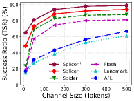
(a) Influence of the channel size

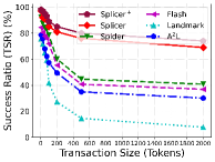
(b) Influence of the transaction size

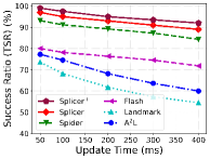
(c) Influence of the update time

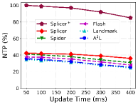
(d) Normalized throughput

Figure 7: The comparison between Splicer⁺ and other schemes without TEE-enabled under different metrics in the small-scale network.

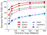
(a) Influence of the channel size

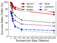
(b) Influence of the transaction size

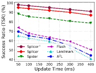
(c) Influence of the update time

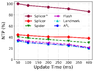
(d) Normalized throughput

Figure 8: The comparison between Splicer⁺ and other schemes without TEE-enabled under different metrics in the large-scale network.

VI-A Experiment Setup

Our evaluation involves simulating with MATLAB and fully implementing the Lightning Network Daemon (LND) testnet. We model the PCN at two scales: a small-scale network (100 nodes) and a large-scale network (3,000 nodes). Our modified LND is deployed on a machine equipped with a six-core i7-9750H processor running at 2.6 GHz (Intel SGX enabled), 32 GB of RAM, 500 GB of SSD storage, and a 10 Gbps network interface. According to Spider’s evaluation benchmark, channel connections between nodes are generated using ROLL [45] following the Watts-Strogatz small-world model. Based on the heavy-tailed distribution observed in real-world datasets regarding lightning channel sizes [46], funds are allocated to each side of the channels. The directional distribution of each transaction is derived from our preprocessed Lightning Network real-world dataset, while transaction values are sourced from the identical credit card dataset [47] employed by Spider. It should be noted that we have confirmed that these transactions are expected to induce some local deadlocks and include high-value transactions beyond the capacity of the Lightning Network.

Parameter settings. The minimum, average, and median channel sizes are 10, 403, and 152 tokens, respectively. The transaction timeout is 3 seconds. Min-TU is 1 token, and Max-TU is 4 tokens. The number $k$ of multiple paths is 5. Management cost $\zeta_{mn}$ is set to $0.02\cdot hops_{mn}$, and synchronization costs $\delta_{nl}$ and $\epsilon_{nl}$ are set to $0.01\cdot hops_{nl}$ and $0.05\cdot hops_{nl}$, respectively, where $hops$ represents the number of hops in the communication path between nodes. In congestion control, the queue size of each channel is set to 8,000 tokens. The factors for the window size $\beta$ and $\gamma$ are 10 and 0.1, respectively. The update time $\tau$ is 200 ms. The threshold $T$ for queue delay is 400 ms. For channel concurrency, the default number of concurrent channels $N_{\rm{CC}}$ is set to 5. The waiting time for batch transactions is 100 ms.

VI-B Performance of Splicer⁺

We want to answer these questions: (i) How does the performance of Splicer⁺ compare to non-TEE-enabled schemes under small/large-scale networks? (ii) How does the performance of Splicer⁺ compare with TEE-enabled schemes? (iii) What is the impact of concurrent channels on the performance?

VI-B1 Comparison with Schemes without TEE-Enabled

We evaluate the performance of Splicer⁺ using various metrics compared to different schemes. As depicted in Fig. 7 and Fig. 8, Splicer⁺ consistently outperforms other schemes across small and large network scales. Splicer [1] is the original solution presented in this paper without TEE support. Spider [12] is a multi-path source routing scheme where each sender determines the routes. Flash [13] is also rooted in source routing, employing a modified max-flow algorithm to discover paths for large payments and randomly routing small payments through precomputed paths. Landmark routing is employed in several previous PCN routing schemes [9, 48, 49]. Each sender calculates the shortest path to well-connected landmark nodes, and then these landmark nodes route to the destination via $k$ distinct shortest paths. The A²L [7] is the state-of-the-art PCH focusing on providing unlinkability. The results are as follows:

Transaction success ratio (TSR) is defined as the number of completed transactions divided by the number of generated transactions. A high TSR value indicates model stability, implying the ability to handle transaction deadlocks and balance network load. Fig. 7(a) and 8(a) demonstrate that Splicer⁺ exhibits an average TSR that is 51.1% higher than the other five schemes. Combining Fig. 7(b) and 8(b), a notable increase (43.6%) in TSR is observed as transaction size varies. These results illustrate that the distributed routing decision protocol of PCHs can enhance the TSR. It is notable that the improvement in Splicer⁺ is more pronounced in large-scale networks. Fig. 7(c) and 8(c) depict the TSR under the influence of update time $\tau$ across different schemes. Longer update times increase the likelihood of fund deadlocks occurring in the PCN. Results indicate that Splicer⁺ maintains a stable TSR above 91% as update time increases, slightly surpassing Spider by 7.2% and 13.8%, respectively. Since Spider also employs a multi-path routing strategy, reducing deadlock possibilities, TSR remains high when channel size is suitable. Conversely, the TSR of A²L decreases notably, while Splicer⁺ improves by 38.8% and 60.3%, respectively. Spider conducts source routing computations at end-users, constrained by single machine performance, resulting in lower TSR compared to Splicer⁺, particularly in large-scale networks. Due to A²L’s complex cryptographic primitives limiting scalability, Splicer⁺ exhibits an overall TSR that is 78.2% higher on average. Splicer⁺ further enhances the overall TSR by an average of 6.3% compared to Splicer. This is due to the concurrent channels established by Splicer⁺ between PCHs, which further enable network funds to flow smoothly and nearly without encountering deadlocks.

Normalized throughput (NTP) represents the total value of completed payments relative to the total generated value, normalized by the maximum throughput. Normalization aims to eliminate scale differences between different schemes, facilitating easier comparison. A high NTP value indicates the model’s capability for handling massive concurrent transactions and further validates TSR, confirming the model’s stability. Fig. 7(d) and 8(d) illustrate that the NTP of Splicer⁺ averages 181.5% higher than the other five schemes. The improvement in throughput by Splicer⁺ is more pronounced in large-scale networks (average of 189.3%).Compared to Spider, Splicer⁺ exhibits an average NTP increase of 156% and 161.3%, respectively. In comparison to A²L, Splicer⁺ demonstrates more significant enhancements of 202.5% and 235.4%, respectively. With increasing update time, more transactions approach their deadlines, leading to a higher probability of transaction failure. Due to the absence of a scalable routing strategy design, A²L is more susceptible to this factor. On average, Splicer⁺ exhibits a further 130.9% increase in overall NTP compared to Splicer. This is primarily attributed to the performance advantage of concurrent channels between TEE-enabled PCHs, further reducing the burden of highly concurrent transactions. Hence, taking into account TSR and throughput, we select the median of 200 ms as the update time for Splicer⁺.

The aforementioned results demonstrate that Splicer⁺ can markedly enhance performance scalability compared to state-of-the-art techniques without TEE support. In large-scale networks, the impact of Splicer⁺ on performance enhancement is more pronounced. Moreover, Splicer⁺’s placement optimization reduces communication costs (refer to §VI-C). Therefore, in large-scale low-power scenarios, we suggest adopting Splicer⁺ if TEE support is available; otherwise, Splicer is recommended.

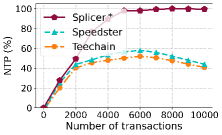
(a) Normalized throughput

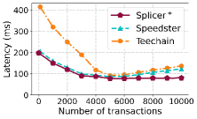
(b) Transaction latency

Figure 9: The comparison between Splicer⁺ and other TEE-enabled schemes.

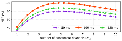
Figure 10: Performance evaluation of concurrent channels.

VI-B2 Comparison with TEE-enabled Schemes

We observe the normalized throughput and latency of different schemes under the stress test of 10,000 transactions per initiation. The mean values of the results tested under two network scales are shown in Fig. 9. Both Teechain [20] and Speedster [19] employ TEE to ensure transaction security in PCNs and to improve performance. The primary distinction from Splicer⁺ lies in their non-utilization of PCHs for distributed routing decisions.

The results depicted in Fig. 9(a) indicate that the average throughput of Splicer⁺ surpasses that of Speedster and Teechain by 72.6% and 90.9%, respectively. Prior to the transaction volume reaching 2,000, all three schemes exhibit rapid increases in throughput, indicating strong concurrent processing capabilities. Nevertheless, once the transaction volume surpasses 2,000, the growth rate of Speedster and Teechain decelerates, eventually declining after peaking at around 6,000 transactions. They exhibit inefficiency in managing extensive multi-hop transactions. Splicer⁺ continues to experience throughput growth even under high transaction loads, stabilizing only after reaching peak throughput.

Results presented in Fig. 9(b) illustrate that initially, transaction latency decreases with increasing transaction volume across all three schemes. This phenomenon is attributed to their ability to process transactions concurrently, enabling them to handle a greater number of transactions per unit of time. However, once the transaction volume surpasses 5,000, the latency of Speedster and Teechain begins to rise due to the resource-intensive nature of processing extensive transactions, resulting in prolonged processing times for complex transactions that require forwarding through multiple nodes. Due to Splicer⁺ leveraging PCHs for routing computations, it effectively mitigates the client’s constraints in handling extensive multi-hop complex transactions.

In summary, the results demonstrate that Splicer⁺ maintains high throughput and low latency levels even with increasing transaction volumes, validating the efficacy of outsourcing routing computation and decentralized routing decisions employing PCHs.

VI-B3 Performance Benefits of Concurrent Channels

The normalized peak throughput for various numbers of concurrent channels ($N_{CC}$) is observed, as depicted in Fig. 10. NTP exhibits an initial increase followed by a decrease with the rise in $N_{CC}$ for varying batch transaction waiting times. This indicates a tuning optimization process. Initially, augmenting $N_{CC}$ enhances the system’s concurrent processing capability, subsequently boosting NTP. Nevertheless, with continued increments in $N_{CC}$, resource contention intensifies, leading to system overload and inefficient request processing, thereby diminishing NTP. Regarding waiting time, NTP is lower for both 50 ms and 150 ms compared to 100 ms. Despite having more time to process requests when the wait time is 150 ms, NTP is adversely affected by resource contention and load imbalance. Hence, we default to setting 5 concurrent channels. Additionally, experimental results corroborate the CCBT proposed in §IV-E.

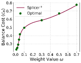
(a) Balance cost

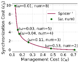
(b) Tradeoff in costs

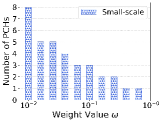
(c) Small-scale networks

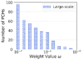
(d) Large-scale networks

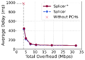
(e) Costs in the small-scale network

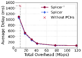
(f) Costs in the large-scale network

Figure 11: Evaluation of smooth node placement.

TABLE III: The influence of the different choices in routing for Splicer⁺.

Scale	Path Type				Path Number				Scheduling Algorithm
	KSP	Heuristic	EDW	EDS	1	3	5	7	FIFO	LIFO	SPF	EDF
Small	66.41%	77.83%	86.37%	82.14%	34.54%	72.38%	88.54%	83.74%	53.81%	90.35%	76.18%	70.44%
Large	59.53%	76.32%	91.63%	85.16%	36.76%	67.29%	92.29%	86.30%	63.48%	95.40%	83.19%	80.48%

VI-C Evaluation of Smooth Node Placement

Next, in Fig. 11, we evaluate the placement of smooth nodes and investigate: (i) How about the efficiency tradeoff of the placement? (ii) How effective is the placement?

Efficiency tradeoff. Fig. 11(a) and 11(b) illustrate the impact of weight values on costs in the small-scale network. Fig. 11(a) demonstrates how the average balance cost of running the PCHs fluctuates with the weight value $\omega$ defined in §IV-B. Overall, our model’s performance closely approaches the optimum for nearly all $\omega$ values. This indicates the successful simulation of the network’s two communication costs by our model. Furthermore, Fig. 11(b) illustrates the tradeoff between the two costs. The nodes in the figure are annotated with their respective weight $\omega$ and the number of smooth nodes (e.g., 4 smooth nodes for $\omega=0.04$). Management costs occur between smooth nodes and clients, while synchronization costs are exclusively between smooth nodes. PCNs have varying affordability for these two costs. For instance, due to the robust computational capacity of the PCHs, PCNs can tolerate high synchronization costs. Clients may consist of IoT nodes, allowing PCNs to incur lower management costs. Hence, based on these findings, Splicer⁺ can effectively adjust both costs by adjusting the number of smooth nodes in the voting smart contract. Additionally, the curves depicting the influence of weight values on costs in large-scale networks resemble those in small-scale networks. However, large-scale networks necessitate a greater number of smooth nodes compared to small-scale networks. Fig. 11(c) and 11(d) illustrate the number of smooth nodes for various weight values $\omega$ in small and large network scales. In scenarios where management cost takes precedence, Splicer⁺ deploys additional smooth nodes to minimize communication overhead and latency for managing clients, and vice-versa.

Placement effectiveness. Fig. 11(e) and 11(f) illustrate the average transaction delay and total traffic overhead with and without PCHs, showcasing the effectiveness of smooth nodes by comparing distributed routing and source routing decisions. The delay-overhead curves are depicted by iterating through weight values in both small and large-scale networks. In the absence of smooth nodes, the average delay and traffic overhead remain constant. Despite similar total overhead, Splicer⁺ exhibits significantly lower average delay compared to scenarios without smooth nodes. Overall, Splicer⁺ achieves 72% lower latency compared to schemes lacking PCHs, such as Spider. On average, Splicer⁺ introduces only an additional 5.5% delay due to TEE compared to Splicer, which is negligible compared to scenarios without PCHs. Strategically placing certain PCHs can decrease the network’s overall overhead. Furthermore, Splicer⁺ can accommodate additional traffic overhead to further reduce transaction latency.

VI-D Routing Choices in Splicer⁺

Lastly, we evaluate and select the optimal: (i) Type of routing paths, (ii) Number of routing paths, and (iii) Route scheduling strategy. Given the paper’s emphasis on reducing transaction deadlocks, Table III illustrates the impact of various routing choices on TSR.

Path type. We assess performance by selecting various types of routing paths for each source-destination pair in two network scales. KSP refers to the k-shortest paths. The heuristic method selects 5 feasible paths with the highest channel funds. EDW denotes the edge-disjoint widest paths, while EDS represents the edge-disjoint shortest paths. Results indicate that EDW outperforms other approaches in both network scales. Given the heavy-tailed distribution of channel sizes, the widest paths can effectively utilize the network’s capacity.

Path number. We assess performance across different numbers of EDW paths. The TSR rises with an increasing number of paths, indicating that a greater number of paths more effectively utilize the network’s capacity. However, it is observed that the TSR experiences a slight decline when the number of paths reaches 7, attributed to the high computational complexity introducing a performance bottleneck. Consequently, Splicer⁺ adopts 5 routing paths.

Scheduling algorithm. We modify the scheduling methods for the waiting queue, considering four approaches: first in first out (FIFO), last in first out (LIFO), smallest payments first (SPF), and earliest deadline first (EDF). The findings indicate that LIFO yields 10-40% higher performance compared to other methods as it prioritizes transactions farther from their deadlines. FIFO and EDF prioritize transactions nearing their deadlines, resulting in poorer transaction performance due to increased failures. Although SPF exhibits the second-best performance, the accumulation of large transactions consumes significant channel funds, thereby reducing the transaction success ratio. Consequently, we opt for the LIFO strategy.

In practical applications, the aforementioned routing choices can be tailored to suit various scenarios and accommodate different demand patterns.

VII Related Work

PCH schemes: TumbleBit [6] proposes a cryptographic protocol designed for PCH that reduces routing complexity by maintaining multiple channels and enables unlinkability of transactions. A limitation is that it relies on scripting functionality, and its communication complexity grows linearly with increasing security parameters. A²L [7] introduces a new cryptographic primitive to optimize TumbleBit, designed to improve backward compatibility and efficiency. Similar improvements have been made by BlindHub [14] and Accio [15]. Commit-chains [17] take a similar approach to processing off-chain transactions as PCH, i.e., serving multiple users through a centralized operator, with tradeoffs in channel construction costs, subscriber churn, funds management, and decentralization. Perun [16] uses a smart contract-based approach to constructing virtual PCHs with the aim of reducing communication complexity, but does so at the expense of unlinkability of transactions. Boros [50] proposes a channel-oriented PCH to shorten the routing path of PCN. However, these works do not consider the problem of PCH placement options, which has a significant impact on the transaction delay and communication cost of PCNs.

Source routing schemes for PCNs: Flare[9] introduces a hybrid routing algorithm whose goal is to improve the efficiency of payment route lookup. Revive [11] presents the first fund rebalancing scheme in PCNs that is able to adjust for channels with unevenly distributed funds. But it relies on a routing algorithm that requires the involvement of a trusted third party, which could leave the system vulnerable to the risk of a single point of attack. Sprites [10] works to reduce the worst-case collateralization cost of off-chain transactions. Spider [12] proposes a packet-based multi-path routing scheme aiming at high throughput routing in PCNs. However, this requires the senders to compute the paths to the receivers, which may place high demands on the performance of the senders in large-scale PCN environments. Meanwhile, other layer-2 solutions have emerged on Ethereum, such as Rollups [51, 52], which batch-processes transactions to increase system throughput, albeit with increased latency. However, this is beyond the scope of our discussion about the PCN architecture.

TEE-based PCN schemes: Teechan [18] exploits TEE to build a one-hop payment channel framework to achieve secure scalability. Teechain [20] proposes a secure PCN with asynchronous blockchain access based on Teechan. Speedster [19] provides a secure account-based state channel system with TEE. However, they rely too much on TEE. Every user in PCNs must be TEE-enabled, limiting the scope of applications for clients, though Teechain can use outsourced remote TEE-enabled nodes. Splicer⁺ breaks this limitation on clients. Twilight [53] utilizes TEE-enabled relay nodes to provide differential privacy protection for PCN users, but it also increases the computational and communication overhead, especially in large-scale networks, which can result in performance degradation or increased communication latency.

VIII Conclusion and Future Work

We propose an innovative PCH solution called Splicer⁺ that aims to explore a new balance between decentralization, scalability, and security. In particular, we develop a novel, TEE-based PCH node, the smooth node. Among multiple smooth nodes, we introduce a distributed routing mechanism that is highly scalable and capable of routing transaction flows in PCNs with an optimized deadlock-free strategy. We address the problem of PCH placement for network scalability and propose solutions for small to large networks, respectively. To enhance the performance scalability, we implement a rate-based routing and congestion control protocol for PCHs. Based on multi-path routing and confidential computation of TEE, Splicer⁺ provides strong privacy protection for off-chain transactions. We formalize the security definition and proof of the Splicer⁺ protocol in the UC-framework. Evaluations on different scale networks show that Splicer⁺ effectively balances the network load and outperforms existing state-of-the-art techniques on transaction success ratio, throughput, and resource cost.

Our research on secure off-chain PCH has only advanced a small step, and there is still a long way to go. PCH can be further improved and innovated in many aspects, such as more efficient routing and asynchronous PCH protocols.

Lingxiao Yang (Graduate Student Member, IEEE) received B.E. degree in network engineering from Xidian University in 2018. He is a member of the Shaanxi Key Laboratory of Network and System Security. He is currently pursuing the Ph.D. degree with the School of Computer Science and Technology, Xidian University, Xi’an, China. His research interests include Web3 and blockchain applications.

Xuewen Dong (Member, IEEE) received the B.E., M.S., and Ph.D. degrees in computer science and technology from Xidian University, Xi’an, China, in 2003, 2006, and 2011, respectively. From 2016 to 2017, he was with Oklahoma State University, Stillwater, OK, USA, as a Visiting Scholar. He is currently a Professor with the School of Computer Science and Technology, Xidian University. His research interests include cognitive radio network, wireless network security, and blockchain.

Wei Wang (Member, IEEE) is a full Professor with school of computer science and technology, Beijing Jiaotong University, China. He received the Ph.D. degree from Xi’an Jiaotong University, in 2006. He was a Post-Doctoral Researcher with the University of Trento, Italy, from 2005 to 2006. He was a Post-Doctoral Researcher with TELECOM Bretagne and with INRIA, France, from 2007 to 2008. He was also a European ERCIM Fellow with the Norwegian University of Science and Technology (NTNU), Norway, and with the Interdisciplinary Centre for Security, Reliability, and Trust (SnT), University of Luxembourg, from 2009 to 2011. His recent research interests lie in data security and privacy-preserving computation. He has authored or co-authored over 100 peer-reviewed articles in various journals and international conferences, including IEEE TDSC, IEEE TIFS, IEEE TSE, ACM CCS, AAAI, Ubicomp, IEEE INFOCOM. He has received the ACM CCS 2023 Distinguished Paper Award. He is an Elsevier “highly cited Chinese Researchers”. He is an Associate Editor for IEEE Transactions on Dependable and Secure Computing, and an Editorial Board Member of Computers & Security and of Frontiers of Computer Science. He is a vice chair of ACM SIGSAC China.

Sheng Gao (Member, IEEE) received the B.S. degree in information and computation science from the Xi’an University of Posts and Telecommunications in 2009, and the Ph.D. degree in computer science and technology from Xidian University in 2014. He is currently a Professor with the School of Information, Central University of Finance and Economics. He has published over 30 articles in refereed international journals and conferences. His current research interests include data security, privacy computing, and blockchain technology.

Qiang Qu is a Professor with the University of Chinese Academy of Sciences, with Shenzhen Institute of Advanced Technology, Chinese Academy of Sciences. He is currently the Director of Blockchain Laboratory of Huawei Cloud Tech Company Ltd. His research interests include blockchain and data intensive systems.

Wensheng Tian is currently a Researcher with the Nanhu laboratory, China. His current research interests include machine learning, security, and privacy.

Yulong Shen (Member, IEEE) received the B.S. and M.S. degrees in computer science and the Ph.D. degree in cryptography from Xidian University, Xi’an, China, in 2002, 2005, and 2008, respectively. He is currently a Professor with the School of Computer Science and Technology, Xidian University, where he is also an Associate Director of the Shaanxi Key Laboratory of Network and System Security and a member of the State Key Laboratory of Integrated Services Networks. His research interests include wireless network security and cloud computing security. He has also served on the technical program committees of several international conferences, including ICEBE, INCoS, CIS, and SOWN.

References

- [1] L. Yang, X. Dong, S. Gao, Q. Qu, X. Zhang, W. Tian, and Y. Shen, “Optimal hub placement and deadlock-free routing for payment channel network scalability,” in 2023 IEEE 43rd International Conference on Distributed Computing Systems (ICDCS). IEEE, 2023, pp. 692–702.
- [2] S. Werner, D. Perez, L. Gudgeon, A. Klages-Mundt, D. Harz, and W. Knottenbelt, “Sok: Decentralized finance (defi),” in 4th ACM Conference on Advances in Financial Technologies, 2022, pp. 30–46.
- [3] L. Heimbach, Q. Kniep, Y. Vonlanthen, and R. Wattenhofer, “Defi and nfts hinder blockchain scalability,” in International Conference on Financial Cryptography and Data Security. Springer, 2023, pp. 291–309.
- [4] The Bitcoin Lightning Network: Scalable Off-Chain Instant Payments. [Online]. Available: {https://lightning.network/lightning-network-paper.pdf}
- [5] Raiden network. [Online]. Available: {https://raiden.network}
- [6] E. Heilman, L. Alshenibr, F. Baldimtsi, A. Scafuro, and S. Goldberg, “Tumblebit: An untrusted bitcoin-compatible anonymous payment hub.” in NDSS, 2017.
- [7] E. Tairi, P. Moreno-Sanchez, and M. Maffei, “A2l: Anonymous atomic locks for scalability in payment channel hubs,” in 2021 IEEE Symposium on Security and Privacy (SP), 2021, pp. 1834–1851.
- [8] Eosio blockchain. [Online]. Available: {https://eos.io/}
- [9] M. S. A. O. Pavel Prihodko, Slava Zhigulin and O. Osuntokun, “Flare: An approach to routing in lightning network,” 2016.
- [10] A. Miller, I. Bentov, S. Bakshi, R. Kumaresan, and P. McCorry, “Sprites and state channels: Payment networks that go faster than lightning.” in Financial Cryptography, ser. Lecture Notes in Computer Science, vol. 11598. Springer, 2019, pp. 508–526.
- [11] R. Khalil and A. Gervais, “Revive: Rebalancing off-blockchain payment networks,” in Proceedings of the 2017 ACM SIGSAC Conference on Computer and Communications Security, ser. CCS ’17, 2017, p. 439–453.
- [12] V. Sivaraman, S. B. Venkatakrishnan, K. Ruan, P. Negi, L. Yang, R. Mittal, G. Fanti, and M. Alizadeh, “High throughput cryptocurrency routing in payment channel networks,” in NSDI, 2020.
- [13] P. Wang, H. Xu, X. Jin, and T. Wang, “Flash: efficient dynamic routing for offchain networks.” in CoNEXT. ACM, 2019, pp. 370–381.
- [14] X. Qin, S. Pan, A. Mirzaei, Z. Sui, O. Ersoy, A. Sakzad, M. F. Esgin, J. K. Liu, J. Yu, and T. H. Yuen, “Blindhub: Bitcoin-compatible privacy-preserving payment channel hubs supporting variable amounts,” in 2023 IEEE Symposium on Security and Privacy (SP). IEEE, 2023, pp. 2462–2480.
- [15] Z. Ge, J. Gu, C. Wang, Y. Long, X. Xu, and D. Gu, “Accio: Variable-amount, optimized-unlinkable and nizk-free off-chain payments via hubs,” in Proceedings of the 2023 ACM SIGSAC Conference on Computer and Communications Security, 2023, pp. 1541–1555.
- [16] S. Dziembowski, L. Eckey, S. Faust, and D. Malinowski, “Perun: Virtual payment hubs over cryptocurrencies,” in 2019 IEEE Symposium on Security and Privacy (SP), 2019, pp. 106–123.
- [17] R. Khalil, “Commit-chains: Secure, scalable off-chain payments,” 2019.
- [18] J. Lind, I. Eyal, P. R. Pietzuch, and E. G. Sirer, “Teechan: Payment channels using trusted execution environments.” CoRR, 2016.
- [19] J. Liao, F. Zhang, W. Sun, and W. Shi, “Speedster: An efficient multi-party state channel via enclaves,” in Proceedings of the 2022 ACM on Asia Conference on Computer and Communications Security, ser. ASIA CCS ’22, 2022, p. 637–651.
- [20] J. Lind, O. Naor, I. Eyal, F. Kelbert, E. G. Sirer, and P. R. Pietzuch, “Teechain: a secure payment network with asynchronous blockchain access.” in SOSP, 2019, pp. 63–79.
- [21] J. Lee, S. Kim, S. Park, and S.-M. Moon, “RouTEE: A secure payment network routing hub using trusted execution environments,” arXiv preprint arXiv:2012.04254, 2020.
- [22] Q. Wang, Y. Zhang, Z. Bao, W. Shi, H. Lei, H. Liu, and B. Chen, “SorTEE: Service-Oriented Routing for Payment Channel Networks With Scalability and Privacy Protection,” IEEE Transactions on Network and Service Management, vol. 19, no. 4, pp. 3764–3780, 2022.
- [23] R. Canetti, “Universally composable security: A new paradigm for cryptographic protocols,” Cryptology ePrint Archive, Report 2000/067, 2000, https://ia.cr/2000/067.
- [24] I. Anati, S. Gueron, S. Johnson, and V. Scarlata, “Innovative technology for cpu based attestation and sealing,” 2013.
- [25] Lightning Network Daemon. [Online]. Available: {https://github.com/lightningnetwork/lnd}
- [26] R. Gennaro, S. Jarecki, H. Krawczyk, and T. Rabin, “Secure distributed key generation for discrete-log based cryptosystems.” in EUROCRYPT, vol. 1592, 1999, pp. 295–310.
- [27] P. Li, T. Miyazaki, and W. Zhou, “Secure balance planning of off-blockchain payment channel networks.” in INFOCOM. IEEE, 2020, pp. 1728–1737.
- [28] Z.-L. Ge, Y. Zhang, Y. Long, and D. Gu, “Shaduf: Non-cycle payment channel rebalancing,” in NDSS, 2022.
- [29] L. E. Celis, L. Huang, and N. K. Vishnoi, “Multiwinner voting with fairness constraints.” in IJCAI, 2018, pp. 144–151.
- [30] R. Bredereck, P. Faliszewski, A. Igarashi, M. Lackner, and P. Skowron, “Multiwinner elections with diversity constraints.” in AAAI, 2018, pp. 933–940.
- [31] K. Murdock, D. Oswald, F. D. Garcia, J. V. Bulck, D. Gruss, and F. Piessens, “Plundervolt: Software-based fault injection attacks against intel sgx.” in IEEE Symposium on Security and Privacy. IEEE, 2020, pp. 1466–1482.
- [32] S. Fei, Z. Yan, W. Ding, and H. Xie, “Security vulnerabilities of SGX and countermeasures: A survey,” ACM Computing Surveys (CSUR), vol. 54, no. 6, pp. 1–36, 2021.
- [33] Q. Qin, K. Poularakis, G. Iosifidis, and L. Tassiulas, “Sdn controller placement at the edge: Optimizing delay and overheads.” in INFOCOM. IEEE, 2018, pp. 684–692.
- [34] V. P. Il’ev, “An approximation guarantee of the greedy descent algorithm for minimizing a supermodular set function.” Discret. Appl. Math., vol. 114, no. 1-3, pp. 131–146, 2001.
- [35] M. Feldman, J. Naor, and R. Schwartz, “Nonmonotone submodular maximization via a structural continuous greedy algorithm - (extended abstract).” in ICALP (1), ser. Lecture Notes in Computer Science, vol. 6755. Springer, 2011, pp. 342–353.
- [36] N. Buchbinder, M. Feldman, J. Naor, and R. Schwartz, “A tight linear time (1/2)-approximation for unconstrained submodular maximization.” SIAM J. Comput., vol. 44, no. 5, pp. 1384–1402, 2015.
- [37] F. P. Kelly and T. Voice, “Stability of end-to-end algorithms for joint routing and rate control.” Computer Communication Review, vol. 35, no. 2, pp. 5–12, 2005.
- [38] F. Kelly and T. Voice, “Stability of end-to-end algorithms for joint routing and rate control,” ACM SIGCOMM Computer Communication Review, vol. 35, no. 2, pp. 5–12, 2005.
- [39] D. P. Palomar and M. Chiang, “A tutorial on decomposition methods for network utility maximization,” IEEE Journal on Selected Areas in Communications, vol. 24, no. 8, pp. 1439–1451, 2006.
- [40] S. Ha, I. Rhee, and L. Xu, “Cubic: a new tcp-friendly high-speed tcp variant.” ACM SIGOPS Oper. Syst. Rev., vol. 42, no. 5, pp. 64–74, 2008.
- [41] N. J. Gunther, Guerrilla capacity planning - a tactical approach to planning for highly scalable applications and services. Springer, 2007.
- [42] S. Matetic, M. Ahmed, K. Kostiainen, A. Dhar, D. Sommer, A. Gervais, A. Juels, and S. Capkun, “ROTE: Rollback protection for trusted execution,” in 26th USENIX Security Symposium (USENIX Security 17), 2017, pp. 1289–1306.
- [43] R. Pass, E. Shi, and F. Tramèr, “Formal abstractions for attested execution secure processors.” in EUROCRYPT, vol. 10210, 2017, pp. 260–289.
- [44] R. Cheng, F. Zhang, J. Kos, W. He, N. Hynes, N. M. Johnson, A. Juels, A. Miller, and D. Song, “Ekiden: A platform for confidentiality-preserving, trustworthy, and performant smart contracts.” pp. 185–200, 2019.
- [45] A. Hadian, S. Nobari, B. Minaei-Bidgoli, and Q. Qu, “Roll: Fast in-memory generation of gigantic scale-free networks.” in SIGMOD Conference, 2016, pp. 1829–1842.
- [46] S. Tikhomirov, P. Moreno-Sanchez, and M. Maffei, “A quantitative analysis of security, anonymity and scalability for the lightning network.” in EuroS&P Workshops, 2020, pp. 387–396.
- [47] Credit Card Fraud Detection. [Online]. Available: {https://www.kaggle.com/mlg-ulb/creditcardfraud}
- [48] G. Malavolta, P. Moreno-Sanchez, A. Kate, and M. Maffei, “Silentwhispers: Enforcing security and privacy in decentralized credit networks.” in NDSS, 2017.
- [49] S. Roos, P. Moreno-Sanchez, A. Kate, and I. Goldberg, “Settling payments fast and private: Efficient decentralized routing for path-based transactions.” in NDSS, 2018.
- [50] J. Zhang, Y. Ye, W. Wu, and X. Luo, “Boros: Secure and efficient off-blockchain transactions via payment channel hub,” IEEE Transactions on Dependable and Secure Computing, vol. 20, no. 1, pp. 407–421, 2021.
- [51] L. T. Thibault, T. Sarry, and A. S. Hafid, “Blockchain scaling using rollups: A comprehensive survey,” IEEE Access, vol. 10, pp. 93 039–93 054, 2022.
- [52] A. Kotzer, D. Gandelman, and O. Rottenstreich, “SoK: Applications of Sketches and Rollups in Blockchain Networks,” IEEE Transactions on Network and Service Management, 2024.
- [53] M. Dotan, S. Tochner, A. Zohar, and Y. Gilad, “Twilight: A differentially private payment channel network,” in 31st USENIX Security Symposium (USENIX Security 22), 2022, pp. 555–570.