[1]\fnmYoshitsugu \surMatsubara
[1]\orgdivComputer and Network Center, \orgnameSaga University, \orgaddress\street1 Honjo-machi, \citySaga-shi, \postcode840-8502, \stateSaga, \countryJapan
Fluctuations in the email size modeled by a log-normal-like distribution
Abstract
A previously established frequency distribution model combining a log-normal distribution with a logarithmic equation describes fluctuations in the email size during send requests. Although the frequency distribution fit was considered satisfactory, the underlying mechanism driving this distribution remains inadequately explained. To address this gap, this study introduced a novel email-send model that characterizes the sending process as an exponential function modulated by noise from a normal distribution. This model is consistent with both the observed frequency distribution and the previously proposed frequency distribution model.
keywords:
Email size, Power-law fluctuations, Log-normal-like distributionpacs:
89.20.Hh, 05.40.-a1 Introduction
The complex structures and dynamic behaviors of internet systems have attracted considerable attention. Phenomena such as scale-free structures [1] and power-law distributions in packet flows [2, 3, 4, 5, 6, 7, 8, 9, 10, 11] during inter-event times have been studied extensively. Studies have investigated power-law correlations in data flow and email send requests [12] during interevent times.
A previous study identified power-law fluctuations in the email size during send requests [13] and proposed a novel model based on a log-normal-like distribution. This distribution effectively captured the power-law characteristics of large email sizes and has been reported in numerous studies [14]. However, the mechanisms underlying log-normal-like distributions remain inadequately explained. To address this gap, the current study proposed a novel email-size generation model to explain these mechanisms. Simulation results from the proposed model demonstrate exhibit strong agreement with observed frequency distributions and the previously proposed frequency distribution model. Furthermore, linguistic principles have been applied to explain the underlying mechanism of the model.
The paper is structured as follows: Section 2 examines the log-normal-like distribution and its connections to relevant linguistic studies. Section 3 presents the proposed email-size generation model and evaluates its fit to both the observed frequency distribution and the frequency distribution model
2 Email size fluctuations
This section summarizes the analysis of email size fluctuations presented in a previous study [13], which examined the frequency distribution of email sizes across various periods and user groups from May 1, 2015, to July 31, 2015. Two inflection points were identified in the size-frequency distribution, approximately and . The analysis focused on emails with attachments, as plain text emails typically remained below a few tens of kilobytes. The size-frequency distribution was categorized into two subdistributions based on content type, namely “No attachment” and “Attachment,” where “No attachment” refers to plain text and HTML emails. Content types were defined according to the multipurpose internet mail extensions (MIME) protocol [15, 16, 17, 18, 19, 20].
Because email bodies consist of written sentences, linguistic principles were incorporated into the analysis. Most users in the organization from which the data were collected were Japanese, and emails were predominantly written in Japanese and English. Linguistic studies analyzing sentence length have identified several distribution types, including log-normal [21, 22], gamma [23], and hyper-Pascal distributions [24].
Based on this analysis, we proposed a novel model to explain the email size frequency distribution within each subdistribution. The proposed model was evaluated for its goodness of fit with the observed data.
The model is defined by a probability density function for each subdistribution of email size frequencies (where is measured in units of 100 bytes) as follows:
| (1) |
where is the normalized constant (), , and 111.and the function is continuous over the range () for . Eq. 1 integrates the log-normal distribution with ..
The expected value of remained undefined. The logarithms in eq. 1 for can be approximated as follows:
where does not exhibit power-law behavior for . Consequently, influences the power-law properties of when .
The least-squares method was used to evaluate the goodness-of-fit of the proposed model to the observed data in accordance with a previous study [13]. The method is defined as follows:
| (2) |
where represents the relative frequency of each bin size in the observed data and corresponds to the relative frequency derived from the proposed model. We used as the relative frequency by adjusting the normalization constant a and the size range for each bin. approaches zero when . The parameter values and of that minimized were selected for the model.
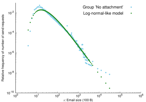
The fitted distribution obtained using the proposed model (eq. 1) for the “No attachment” case is depicted in fig. 1. The parameter values for the fitted curves were and . The model fits the observed data well (fig. 1).
3 Email size generation model
Let denote the email size at time . The size is described by the following equation:
| (3) |
where and are coefficients and represents noise following a normal distribution .
Equation 3 can be interpreted as follows:
-
1.
The email size is influenced by the length of the email body, which is proportional to the sentence length. A direct relationship exists between the text length and email size.
-
2.
The body content is written in natural languages such as English or Japanese.
-
3.
corresponds to the length of a single word.
-
4.
corresponds to the length of a single sentence. Each sentence includes at least one word, with word choice depending on the sentence’s meaning and structure. Additive processes are unlikely because words are not selected randomly. Therefore, represents a multiplicative process [26].
-
5.
corresponds to the length of a compound sentence. A compound sentence consists of at least one single sentence. Sentence selection also depends on meaning and structure, precluding independent random selection. Therefore, the exponential form is used to model this multiplicative process.
-
6.
represents the effect of prior emails. Some emails contained quoted content from previous emails, referred to as the quotation effect. If , then is described as
(4) as a simple case. When , most emails are independent of prior emails. Although some emails contain quoted content, its inclusion has a negligible effect on the size-frequency distribution.
4 Discussion
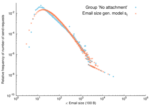
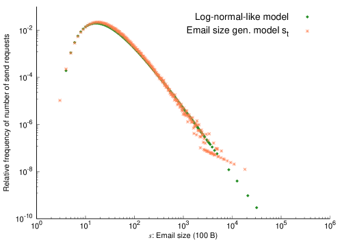
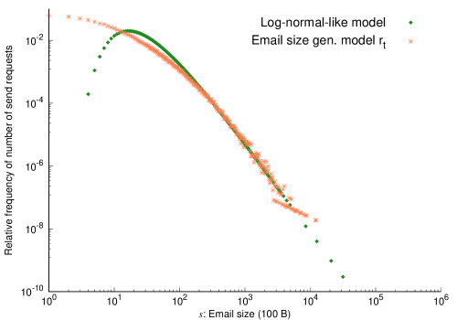
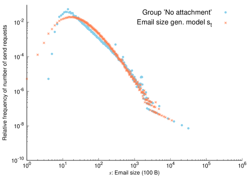
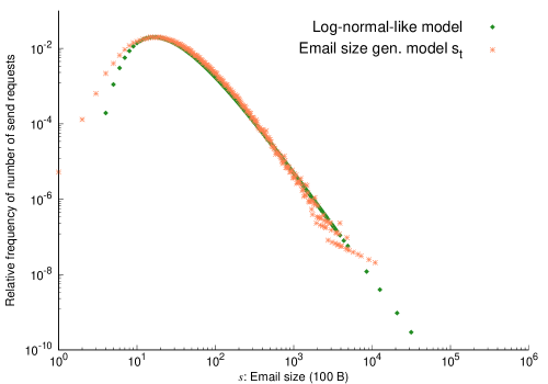
The email size frequency distribution generated using st was simulated, and the results are presented in fig. 2 and fig. 3. This study generated 191,993 emails based on , matching the number of “No attachment” emails analyzed in the previous study [13]. The parameter value of for was , which is the simplest case in eq. 4. The other parameter values for were , , and . The least-squares method denoted by was used to assess the goodness-of-fit. The degree of fitting was each and . The frequency distribution of emails generated by revealed a strong fit to both the observed data and the email size frequency model .
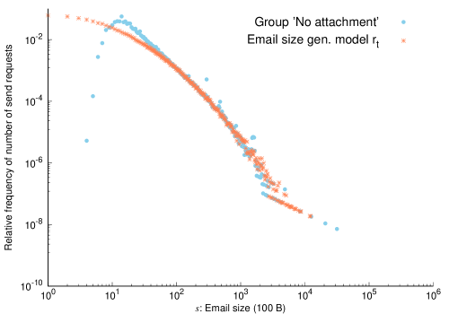
Additionally, the frequency distribution of emails generated using was simulated for comparison. The equation is described as follows:
| (5) |
The fitting results are displayed in fig. 4 and fig. 5. The parameter values for were , , and . The degree of fitting was each and . The fit obtained with was inferior to that of . Therefore, the form represents the log-normal-like distribution.
Next, the fitting for was simulated as an example of . The fitting results are depicted in fig. 6 and fig. 7. The other parameter values for were , , and . The degree of fitting was each and . The fitting was better than that of . However, for , the fitting did not improve compared with that of . These results suggests that most emails are independent of each other.
5 Conclusion
A previous study analyzed the frequency distributions of email sizes in sent requests [13] and proposed a log-normal-like model that combined the log-normal distribution and , where denotes the email size. The proposed model approximates the power-law correlations when . Although prior studies focused on explaining email size fluctuations, they did not sufficiently elucidate the mechanism underlying the generation of these frequency distributions.
To address this gap, this study proposed a novel email size generation model, , to explain the mechanism of the size–frequency distribution . The model equation, , incorporates normal distribution noise . This model is explained based on linguistic principles. The frequency distribution generated using demonstrated a strong fit to both the observed data and the email size frequency model . Simulations with reveal that the log-normal-like distribution, derived from , and the observed email data from the previous study indicate that most emails are independent of each other.
The normal distribution is used as noise in eq. 3. Here, corresponds to the length of a single word in a sentence. The length of one word should be at least one character (one byte). However, the normal distribution theoretically allows negative values. This study explained the email size frequency distribution. A simpler and more effective explanatory model than the current model should be developed using a different distribution in future research.
Compliance with ethical standards
The author has no competing interests to declare that are relevant to the content of this article.
Data Availability Statement
The data are not publicly available to avoid compromising the privacy of the information.
Acknowledgments
The author thanks Makoto Otani, Computer and Network Center, Saga University, for assisting with data collection and analysis.
References
- \bibcommenthead
- [1] M. Faloutsos, P. Faloutsos, C. Faloutsos, On power–law relationships of the internet topology. SIGCOMM Comput. Commun. Rev. 29(4), 251–262 (1999). 10.1145/316194.316229
- [2] V. Paxson, S. Floyd, Wide area traffic: the failure of Poisson modeling. IEEE/ACM Trans. Networking 3, 226–244 (1995). 10.1109/90.392383
- [3] I. Csabai, 1/f noise in computer network traffic. J. Phys. A: Math. Gen. 27(12), L417 (1994). 10.1088/0305-4470/27/12/004
- [4] M. Takayasu, H. Takayasu, T. Sato, Critical behaviors and noise in information traffic. Physica A 233, 824–834 (1996). 10.1016/S0378-4371(96)00189-6
- [5] S. Tadaki, Power-law fluctuation in internet traffic. J. Phys. Soc. Jpn. 76(3), 044001–044001–5 (2007). 10.1143/jpsj.76.044001
- [6] J.P. Eckmann, E. Moses, D. Sergi, Entropy of dialogues creates coherent structures in e-mail traffic. Proc. Nattl. Acad. Sci. U.S.A. 101(40), 14333–14337 (2004). 10.1073/pnas.0405728101
- [7] A.L. Barabási, The origin of bursts and heavy tails in human dynamics. Nature 435, 207–211 (2005). 10.1038/nature03459
- [8] K.I. Goh, A.L. Barabási, Burstiness and memory in complex systems. EPL (Europhys. Lett.) 81(4), 48002 (2008). 10.1209/0295-5075/81/48002
- [9] R.D. Malmgren, D.B. Stouffera, A.E. Motter, L.A.N. Amaral, A Poissonian explanation for heavy tails in e-mail communication. Proc. Natl. Acad. Sci. U.S.A. 105(47), 18153–18158 (2008). 10.1073/pnas.0800332105
- [10] C. Anteneodo, R.D. Malmgren, D.R. Chialvo, Poissonian bursts in e-mail correspondence. Eur. Phys. J. B 75, 389–394 (2010). 10.1140/epjb/e2010-00139-9
- [11] M. Karsai, K. Kaski, A.L. Barabási, J. Kertész, Universal features of correlated bursty behaviour. Sci. Rep. 2, 397 (2012). 10.1038/srep00397
- [12] Y. Matsubara, Y. Hieida, S. Tadaki, Fluctuation in e-mail sizes weakens power-law correlations in e-mail flow. Eur. Phys. J. B 86, 209 (2013). 10.1140/epjb/e2013-40209-x
- [13] Y. Matsubara, Y. Musashi, Fluctuations in email size. Eur. Phys. J. Plus 132, 507 (2017). 10.1140/epjp/i2017-11767-2
- [14] S. Milojevič, Modes of collaboration in modern science: Beyond power laws and preferential attachment. Journal of the American Society for Information Science and Technology 61(7), 1410–1423 (2010). 10.1002/asi.21331
- [15] N. Freed, D.N.S. Borenstein. Multipurpose Internet Mail Extensions (MIME) Part One: Format of Internet Message Bodies. RFC 2045 (1996). 10.17487/RFC2045
- [16] N. Freed, D.N.S. Borenstein. Multipurpose Internet Mail Extensions (MIME) Part Two: Media Types. RFC 2046 (1996). 10.17487/RFC2046
- [17] K. Moore. MIME (Multipurpose Internet Mail Extensions) Part Three: Message Header Extensions for Non-ASCII Text. RFC 2047 (1996). 10.17487/RFC2047. URL https://www.rfc-editor.org/info/rfc2047
- [18] N. Freed, D.N.S. Borenstein. Multipurpose Internet Mail Extensions (MIME) Part Five: Conformance Criteria and Examples. RFC 2049 (1996). 10.17487/RFC2049
- [19] D.J.C. Klensin, N. Freed. Multipurpose Internet Mail Extensions (MIME) Part Four: Registration Procedures. RFC 4289 (2005). 10.17487/RFC4289
- [20] N. Freed, D.J.C. Klensin, T. Hansen. Media Type Specifications and Registration Procedures. RFC 6838 (2013). 10.17487/RFC6838
- [21] H. Arai, Sentence length and lognormal distribution : A case study of akutagawa and dazai. Hitotsubashi Rev. 125(3), 205–223 (2001). http://hermes-ir.lib.hit-u.ac.jp/rs/handle/10086/10418 (In Japanese)
- [22] S. Furuhashi, Y. Hayakawa, Lognormality of the distribution of japanese sentence lengths. J. Phys. Soc. Jpn. 81(3), 034004 (2012). 10.1143/JPSJ.81.034004
- [23] K. Sasaki, Distribution of sentence-length. Math. Linguist. 78, 13–22 (1976). (In Japanese)
- [24] M. Ishida, K. Ishida, On distributions of sentence lengths in Japanese writing. Glottometrics 15, 28–44 (2007). URL https://api.semanticscholar.org/CorpusID:12215774
- [25] S. Milojević, Power law distributions in information science: Making the case for logarithmic binning. J. Am. Soc. Inf. Sci. Technol. 61(12), 2417–2425 (2010). 10.1002/asi.21426
- [26] D.L. Mohr, W.J. Wilson, R.J. Freund, in Statistical Methods (Fourth Edition), ed. by D.L. Mohr, W.J. Wilson, R.J. Freund, 4th edn. (Academic Press, Amsterdam, Netherlands, 2022), pp. 351–444. 10.1016/B978-0-12-823043-5.00008-4