A stabilized finite element method for steady Darcy-Brinkman-Forchheimer flow model with different viscous and inertial resistances in porous media

Abstract

We implement a stabilized finite element method for steady Darcy-Brinkman-Forchheimer model within the continuous Galerkin framework. The nonlinear fluid model, a generalized and sophisticated flow model with inertial effect in porous media, is first linearized using a standard Newton’s method. The sequence of linear problems is then discretized utilizing a stable inf-sup type continuous finite elements based on the Taylor-Hood pair to approximate the primary variables: velocity and pressure. Such a pair is known to be optimal for the approximation of the isotropic Navier-Stokes equation. To overcome the well-known numerical instability in the convection-dominated problems, the Grad-Div stabilization is employed with an efficient augmented Lagrangian-type penalty method. We use the penalty term to develop the block Schur complement preconditioner, which is later coupled with a Krylov-space-based iterative linear solver. In addition, the Kelly error estimator for the adaptive mesh refinement is employed to achieve better numerical results with less computational cost. Performance of the proposed algorithm is verified for a classical benchmark problem, i.e., the 2D lid-driven cavity flow of an incompressible fluid trapped between two plates. Extending the 2D lid-driven cavity flow, a detailed comparative study of the flow nature is presented for a variety of Reynolds number and Darcy number combinations for variety of viscous and inertial resistances. Particularly for the Forchheimer parameter, we present some interesting flow patterns with the velocity components and their streamlines along the mid-lines in the computational domain. The role of the Forchheimer term is highlighted for different porous medium scenarios. This study can offer an attractive setting for discretizing many multi-physics problems along with the fluid flow having inertial effects in porous media.

1 Introduction

Homogenized and simplified from Stoke’s equation, the conventional Darcy’s model can account only for limited instances of flow in porous media. For example, ignoring the inertia effect with low fluid viscosity may not be appropriate to describe real-world problems of convection phenomena (e.g., enhanced oil recovery in petroleum engineering, radioactive waste disposal, extraction, and geothermal energy storage). More details on the limitations of Darcy’s model can be found in [1, 2, 3, 4, 5]. Thus, a sophisticated non-Darcy flow model is required for flow in porous media. Joseph et al. [6] formulated a nonlinear extension of Brinkman’s theory [7] for the flow of a viscous fluid through a swarm of spherical particles, and proposed the Darcy-Brinkman-Forchheimer model [6, 8]. The literature on the application of Darcy-Brinkman-Forchheimer model is quite large: to name a few, experiments on the improvement of heat and mass transfer in porous medium [9, 10, 11], the fuel cell design with the inertial effect of the Forchheimer term [12].

However, the analysis of a nonlinear flow and its modeling are not straightforward in terms of some numerical aspects. Regarding the trapped flow of an incompressible fluid between two parallel plates (henceforth referred as the lid-driven cavity flow), the difficulties may lie in the presence of corner singularities which occur at the points of intersection between the moving lid and other stationary walls; devising a stable numerical discretization method for the model with small viscosity (equivalently, higher Reynolds number); furthermore, a motivation to design highly stable computational algorithms with remarkable accuracy. A more fundamental issue of incompressible fluid flow systems, such as the Navier-Stokes, equivalent to the free fluid for the Darcy-Brinkman-Forchheimer when the $Darcy$ number (i.e., permeability) goes to infinite, is the stabilization of numerical solution. Interested readers can refer the reviews [13, 14] about mathematical issues for the stabilization of the incompressible Navier-Stokes equation. Furthermore, for the convection-dominated incompressible fluid flow problems, it is well known that a naive Galerkin finite element method is known to produce spurious oscillations and numerical instabilities near the corners [15, 16].

For the lid-driven cavity flow, various high-order methods have been proposed to control the oscillations and to achieve the optimal accuracy in the Sobolev space norm [17, 18, 19]. Some studies have reported the semi-analytical solutions for the flow problems with low Reynolds number using the biorthogonal eigenfunctions [20, 21, 22, 23]. For the flow problems with moderate or high Reynolds number in a cavity with a top moving plate, many strategies have been proposed in the literature, some of which include regularizing the whole boundary value problem by altering the top-lid tangential velocity condition to a polynomial that vanishes at the endpoints [24, 25]. However, such methods are computationally expensive, and particularly in [25], the underlying finite element test function space approximating the velocity variable still needs to be far smoother. The Streamline Upwind Petro-Galerkin (SUPG) method is another popular countermeasure to the classical Galerkin finite element formulation that stabilizes the computations for higher Reynolds number [26, 27, 28], and also in compressible flow simulations [29]. An open and challenging issue in the SUPG method is analyzing the coupling between velocity and pressure terms in the discrete variational formulation (see the works in [30, 31] for the issues with SUPG method). Meanwhile, the study from Barragy and Carey [25] used $p$-type finite elements for the vorticity-stream function formulation and reported a highly accurate solution for the steady cavity problem. In Botella and Peyret’s work [32], a Chebyshev collocation method is used for the lid-driven cavity flow problem by subtracting the leading order terms from the asymptotic expansion of the solution to the steady Navier-Stokes equation, where very high-order polynomials are still used in the approximation. Further, many researchers have used the velocity-vorticity formulations rather than computing velocity-pressure as primary variables [33] due to the lack of an independent equation for pressure. However, the boundary conditions for the vorticity variable at the corner of the top lid could be more straightforward.

In this study, we devise a stabilized finite element method for the stationary Darcy-Brinkman-Forchheimer model with incompressible, isotropic, Newtonian fluid filled in porous media, and illustrate its performance through the lid-driven cavity flow problem. Using the stabilized solutions, we also highlight some important flow features – such as the effect of dimensionless constants and the role of the Forchheimer term. To that end, the inf-sup stable finite element approximation and a Grad-Div stabilization is employed with the primary variable pair of velocity-pressure. The Grad-Div stabilization, suggested in various studies [30, 34, 35, 36], is another popular and robust approach to reducing the velocity error due to the pressure error and preserving the mass conservation. Particularly motivated by [37], we employ the product of a stabilization parameter and the Grad-Div term to the momentum equation, where the choice of the stabilization parameter is vital for the accuracy of numerical solutions [38]. An effecient Schur complement-based preconditioner is develped by utilizing the block-strucutre of the discrete system [37]. which reduces the number of Newton iterations and makes the whole process independent of the total degrees of freedom. Besides the preconditioner for the linear solver, the adaptive mesh refinement based on the Kelly error estimator [39] is employed to achieve better numerical results with less computational cost.

To validate our finite element discretization along with the preconditioner and corresponding implementation, the computational code is tested with a manufactured solution for the optimal convergence rate in $H^{1}$- and $L^{2}$-norms, where we report the optimal orders for both velocities and pressure. Our finite element solution is also compared against a finite difference solution in [40] and reports an excellent agreement between the two results. We then perform further numerical experiments for different viscous and inertial resistances in porous media. Two groups of Reynolds and Darcy numbers are set, for which Re $\times$ Da values are less than and greater than 1.0. Regarding the numerical performance, we find the preconditioner-based algebraic penalty term stabilizes the relatively high Reynolds number (up to $1000$). Furthermore, our method takes few iterations within Newton’s method even for the nonlinear model. Due to local mesh adaptivity, the whole procedure is shown to be independent of the degree of freedom and effective for large-scale sparse problem even when Re $\times$ Da are increased. Our study further focuses on the comparison, i.e., the Brinkman and Darcy-Brinkman models without the Forchheimer term with the full nonlinear Darcy-Brinkman-Forchheimer. For two groups of Reynolds and Darcy numbers, the primary, secondary, and tertiary vortices of the models are compared. In the Darcy-Brinkman-Forchheimer model, we identify distinct streamline patterns and the departures from other models in the location and size of primary, secondary, and tertiary vortices. We also highlight the role of Forchheimer term for the turbulent flow regime in the porous medium. The Forchheimer term is found to play its role as the resistance to the inertial force and convection, delaying the flow regime change between the laminar and turbulence regime of flow in porous media.

The paper is organized as follows: Section 2 describes the mathematical model that characterizes the flow of incompressible fluid in a non-Darcy porous medium. Some essential nations from functional analysis, a damped Newton’s method, a corresponding variational formulation, and a stable finite element discretization are described in Section 3. In the same section, a linear solver, preconditioner, and Kelly error indicator-based local mesh refinement are explained in detail. Section 4 contains the numerical experiments using the proposed finite element algorithm. The conclusions and some directions for future works are outlined in Section 5.

2 Governing Equations

For the momentum balance of the steady flow, the following nonlinear equation, i.e., the Darcy-Brinkman-Forchheimer model governs the flow in a fully saturated porous medium when the inertia effects and the fluid incompressibility constraint are considered:

$$\rho\mathbf{u}\cdot\nabla\mathbf{u}+\nabla p =\mu\Delta\mathbf{u}-\phi\frac{\mu}{K}\mathbf{u}-\phi\frac{\rho\,\beta}{\sqrt{K}}\,|\mathbf{u}|^{\alpha}\,\mathbf{u}+\widetilde{\mathbf{f}},\quad{\mbox{in}\quad\Omega}$$ (1a)

$$\nabla\cdot\mathbf{u} =0,\quad{\mbox{in}\quad\Omega},$$ (1b)

where $\mathbf{u}\colon\Omega\to\mathbb{R}^{2}$ is the velocity, $p\colon\Omega\to\mathbb{R}$ is the pressure, in which $\Omega\subset\mathbb{R}^{2}$ is a smooth, bounded, non-convex domain, and $\partial\Omega$ is its boundary. $K$ and $\phi$ are the intrinsic permeability and porosity of the medium, respectively. Also, $\mu$ is the coefficient of dynamic viscosity of the fluid, $\rho$ is the fluid density. $\beta$ is the Forchheimer coefficient, which is a positive quantity for the inertial resistance depending on the geometry of the medium. The symbol $|\cdot|$ is the Euclidean norm, and $|\mathbf{u}|^{2}=\mathbf{u}\cdot\mathbf{u}$. Note that the Forchheimer term has a power, $\alpha$, generally regarded as $1.0\leq\alpha\leq 2.0$ [41, 42]. In this study, we take $\alpha=1.0$, resulting in the quadratic form deviating from the linear Darcy’s law. Moreover, the right hand side term $\widetilde{\mathbf{f}}$ represents an external force (e.g., externally applied magnetic field).

Assuming $\phi=1.0$ for simplicity, we introduce the following dimensionless quantities:

$$\mathbf{x}^{*}=\frac{\mathbf{x}}{L},\quad\mathbf{u}^{*}=\frac{\mathbf{u}}{U_{0}},\quad p^{*}=\frac{p}{\rho\,U_{0}^{2}},$$ (2)

where $L$ and $U_{0}$ are the characteristic properties of length and velocity, respectively. Their scales depend on a problem, and for a porous medium, $L$ is the reference distance (e.g., the mean diameter of grain) and $U_{0}$ denotes the magnitude of the reference discharge relative to the solid grain, having the unit of velocity. We omit the asterisks, $(\cdot)^{*}$, of the dimensionless quantities henceforth for simplicity of the notation. Under the assumption of no external force, the dimensionless equations of motion are as follows:

$$\mathbf{u}\cdot\nabla\mathbf{u}+\nabla p =\underbrace{\frac{1}{Re}}_{\displaystyle(a)}\Delta\mathbf{u}-\underbrace{\frac{1}{Re\,Da}}_{\displaystyle(b)}\,\mathbf{u}-\underbrace{\frac{c_{F}}{\sqrt{Da}}}_{\displaystyle(c)}\,\|\mathbf{u}\|\,\mathbf{u},$$ (3a)

$$\nabla\cdot\mathbf{u} =0,\quad$$ (3b)

where $c_{F}$ is the dimensionless coefficient for inertial resistance. $Re$ and $Da$ are characteristic and dimensionless quantities of the Reynolds and Darcy numbers, respectively, defined as

$$Re =\frac{\rho\,L\,U_{0}}{\mu},$$ (4)

$$Da =\frac{K}{L^{2}}.$$ (5)

As seen in (4), note that the inverse of $Re$ number ($(a)$ in (3a)) is the ratio of viscous force to inertial force for a fluid. Then, the coefficient $(b)\dfrac{1}{Re\,Da}$ in (3a) plays its role as the viscous resistance of the fluid flow through a porous medium, whereas the coefficient $(c)\dfrac{c_{F}}{\sqrt{Da}}$ in (3a) represents the inertial resistance, respectively.

Remark 1.

The Forchheimer term with the power $\alpha$ in (1a) has its basis derived in the framework of the homogenization theory of the pore scales, and it can have various forms (e.g., the cubic form for the weak inertia) [41, 43]. Although the exact value may depend on the physical nature of the model, the validity of the quadratic form was confirmed in [44], through matching with the experimental results [45]. Regarding the inertial resistance (or the Forchheimer) coefficient, there are several methodologies for its determination based on both theoretical and empirical aspects, which depend on the corresponding properties of the porous medium. For example, it can be theoretically determined by employing the Ergun equation [46, 47], while empirically by using a correlation between the coefficient and the permeability, which can result in certain range of values due to the scale difference of environments between the lab and reality. In this study, neither aspects of the theoretical nor empirical backgrounds are utilized, but we fix its value within a typical range, according to the literature.

Remark 2.

Setting the porosity $(\phi)$ value as unity is based on the simplification process, and this framework is the same in its form as the penalization method [48, 42] for fully coupling method between the Navier-Stokes equation and the full nonlinear model, i.e., the Darcy-Brinkman-Forchheimer. Note the resistance terms can also imply porous medium since the resistance can be induced by porosity, i.e., the flow channel, and its property. It can also be viewed as a fictitious domain approach [42, 49, 50] for modeling fluid flow resistance in porous media.

Remark 3.

As for the full nonlinear Darcy-Brinkman-Forchheimer model (3a), some studies (e.g., see [51]) have omitted the Forchheimer term, while other literature (e.g., see [8]) has no convection term. In this study, note that we name an equation as the (linearized) Brinkman model, when

$$\nabla p=\frac{1}{Re}\Delta\mathbf{u}-\frac{1}{Re\,Da}\,\mathbf{u},$$ (6)

whereas the Darcy-Brinkman model, being expressed as

$$\mathbf{u}\cdot\nabla\mathbf{u}+\nabla p=\frac{1}{Re}\Delta\mathbf{u}-\frac{1}{Re\,Da}\,\mathbf{u}.$$ (7)

The only difference between the two models above lies in the nonlinear convective term, $\mathbf{u}\cdot\nabla\mathbf{u}$. Note that the Darcy-Brinkman(-Forchheimer) model is convergent to the Navier-Stokes model when $Da$ goes to large number, ultimately being identical to it, if $Da\rightarrow\infty$.

3 Numerical Methods

In this section, numerical methods employed for the rigorous numerical results of this study are explained. In Section 3.1, some notations about the functional spaces are defined and introduced. The nonlinear governing equations, the Darcy-Brinkman-Forchheimer with the incompressibility constraint, are linearized first using Newton’s method in Section 3.2. The linearized equations are turned into the variational formulation in Section 3.3. In Section 3.4, the stabilized finite element method is introduced, and some preconditioners for the linear solver employed in this study are explained in Section 3.5. Finally, the local adaptive mesh refinement method based on the Kelly error estimator [39] is described in Section 3.6.

3.1 Notations and preliminaries

Throughout this study, we assume $\Omega\subset\mathbb{R}^{2}$ a non-convex, bounded polygonal domain with boundary $\partial\Omega$. Let $X$ be a normed linear space defined for $\Omega$ and $L^{p}\left(X\right)$ is a space of all Leb$\grave{e}$sgue integrable functions defined on $\Omega$, in particular

$$L^{2}\left(\Omega\right):=\left\{q\colon\Omega\to\mathbb{R}\,|\,\int_{\Omega}|q|^{2}d\bm{x}<\infty\right\}$$ (8)

is the classical space of square-integrable functions, and the corresponding inner-product and norm are defined as

$$\left(p,\,q\right):=\int_{\Omega}p\,q\,d\bm{x}\quad\mbox{and}\quad||q||:=\left(\int_{\Omega}|q|^{2}d\bm{x}\right)^{1/2}.$$ (9)

Also, the norm $||\cdot||_{p}$ is defined as

$$||u||_{p}=\left(\int_{\Omega}||u||^{p}_{X}\;d\bm{x}\right)^{1/p},\quad p\in[1,\;\infty).$$ (10)

For the problem on hand, the natural Hilbert space is defined as follows:

$$\mathbf{X}_{0} =H_{0}^{1}\left(\Omega\right)^{2}:=\left\{{\mathbf{v}}\colon\Omega\to\mathbb{R}^{2}\;|\;{\mathbf{v}}\in\left(L^{2}\left(\Omega\right)\right)^{2},\;\nabla{\mathbf{v}}\in\left(L^{2}\left(\Omega\right)\right)^{2\times 2},\;{\mathbf{v}}=\mathbf{0}\;\;\mbox{on}\;\;\partial\Omega\right\},$$ (11)

$$Q_{0} =L_{0}^{2}\left(\Omega\right):=\left\{{q}\in L^{2}\left(\Omega\right)\colon\int_{\Omega}{q}\;d\bm{x}=0\right\},$$ (12)

and further $\mathbf{X}=H^{1}\left(\Omega\right)^{2}$, $Q=L^{2}\left(\Omega\right)$. The $H^{1}$-norm is then defined as

$$\|\mathbf{u}\|_{H^{1}(\Omega)}:=\left(\|\mathbf{u}\|_{2}^{2}+\|\nabla\mathbf{u}\|_{2}^{2}\right)^{1/2}.$$ (13)

3.2 Linearization using Newton’s method

Our main goal in this paper is to propose a stable finite element discretization for the nonlinear partial differential equations (PDEs) system for the Darcy-Brinkman-Forchheimer model described in Section 2. A common strategy for the numerical solution of nonlinear differential equations is to first obtain a sequence of linear problems by using Picard’s or Newton’s method at the PDE level, which is then solved by an appropriate numerical technique [52, 53, 54]. Alternatively, one can discretize the nonlinear partial differential equations and obtain a system of nonlinear algebraic equations, which are then solved by any befitting linear algebra techniques. Both methods are mathematically identical, and there is less likely to be any difference in computational perspective. One can also linearize the continuous variational formulation and then solve the resulting formulation by an appropriate numerical method for convergence. In this work, we linearize at the differential equation level, and then the linear problems are solved using the continuous Galerkin finite element method.

Let $\mathbf{x}^{n}=\left(\mathbf{u}^{n},\;p^{n}\right)$ be a numerical approximation to the primary variables, $\mathbf{u}$ and $p$, and $n$ denotes iterative step number for the Newton’s method. We then write the system (3a)-(3b) by moving all the terms to the left-hand side and obtain

$$F(\mathbf{x}):=F(\mathbf{u},\,p)=\begin{pmatrix}\mathbf{u}\cdot\nabla\mathbf{u}+\nabla p-\dfrac{1}{Re}\,\Delta\mathbf{u}+\dfrac{1}{Re\,Da}\,\mathbf{u}+\dfrac{c_{F}}{\sqrt{Da}}\|\mathbf{u}\|\mathbf{u}\\ -\nabla\cdot\mathbf{u}\end{pmatrix}.$$ (14)

We then see an approximation to $\mathbf{x}^{n}$ of the form

$$\mathbf{x}^{n+1}=\mathbf{x}^{n}+{\widehat{\alpha}}\,\delta\mathbf{x}^{n}.$$ (15)

In (15), the term $\delta\mathbf{x}^{n}$ is known as the update or the correction term, and ${\widehat{\alpha}}$ is a line search parameter that helps to achieve the quadratic convergence property of Newton’s method, for which we use $\alpha=1.0$ in this study. The updates are obtained using

$$\delta\mathbf{x}^{n}=-\left(\nabla F(\mathbf{x}^{n})\right)^{-1}F(\mathbf{x}^{n}),$$ (16)

and $\nabla F(\mathbf{x}^{n})$ denotes the Jacobian of $F(\mathbf{x})$ evaluated at $\mathbf{x}^{n}$. Finally, Newton’s iterative algorithm for the current mixed fields of velocity and pressure can be formulated as a combination of (15) and (16). The equation (16) can also be written as

$$\nabla F(\mathbf{x}^{n})\,\delta\mathbf{x}^{n}=-\,F(\mathbf{x}^{n}).$$ (17)

The term on the left-hand side of (17) is the directional derivative of $F(\mathbf{x}^{n})$ in the direction of $\delta\mathbf{x}^{n}$. We compute the directional derivative by using the basic definition

$$\nabla F(\mathbf{x}^{n})\,\delta\mathbf{x}^{n}=\nabla F(\mathbf{u}^{n},\,p^{n})(\delta\mathbf{u}^{n},\,\delta p^{n})$$ (18)

$$=\lim_{\epsilon\to 0}\frac{F(\mathbf{u}^{n}+\epsilon\delta\mathbf{u}^{n},\,p^{n}+{\epsilon\delta p^{n}})-F(\mathbf{u}^{n},\,p^{n})}{\epsilon}$$ (19)

$$=\begin{pmatrix}\mathbf{u}^{n}\cdot\nabla\delta\mathbf{u}^{n}+\delta\mathbf{u}^{n}\cdot\nabla\mathbf{u}^{n}+\nabla\delta p^{n}-\dfrac{1}{Re}\,\Delta\delta\mathbf{u}^{n}+\dfrac{1}{Re\,Da}\,\delta\mathbf{u}^{n}\\ +\dfrac{c_{F}}{\sqrt{Da}}\left(\|\mathbf{u}^{n}\|\delta\mathbf{u}^{n}+\dfrac{\mathbf{u}^{n}\cdot\delta\mathbf{u}^{n}}{\|\mathbf{u}^{n}\|}\mathbf{u}^{n}\right)\\ \\ -\nabla\cdot\delta\mathbf{u}^{n}\end{pmatrix}.$$ (20)

The resultant linearized PDEs system that is to be solved at every Newton step for $\delta\mathbf{u}^{n}$ and $\delta p^{n}$ reads

$$\begin{pmatrix}\mathbf{u}^{n}\cdot\nabla\delta\mathbf{u}^{n}+\delta\mathbf{u}^{n}\cdot\nabla\mathbf{u}^{n}+\nabla\delta p^{n}-\dfrac{1}{Re}\,\Delta\delta\mathbf{u}^{n}+\dfrac{1}{Re\,Da}\,\delta\mathbf{u}^{n}\\ +\dfrac{c_{F}}{\sqrt{Da}}\left(\|\mathbf{u}^{n}\|\delta\mathbf{u}^{n}+\dfrac{\mathbf{u}^{n}\cdot\delta\mathbf{u}^{n}}{\|\mathbf{u}^{n}\|}\mathbf{u}^{n}\right)\\ \\ -\nabla\cdot\delta\mathbf{u}^{n}\end{pmatrix}\\ =-F(\mathbf{u}^{n},\,p^{n}),$$ (21)

and the right-hand side is given by

$$F(\mathbf{u}^{n},\,p^{n})=\begin{pmatrix}\mathbf{f}^{n}\\ -\nabla\cdot\mathbf{u}^{n}\end{pmatrix},$$ (22)

where $\mathbf{f}^{n}$ denotes

$$\mathbf{f}^{n}=\mathbf{u}^{n}\cdot\nabla\mathbf{u}^{n}+\nabla p^{n}-\dfrac{1}{Re}\,\Delta\mathbf{u}^{n}+\dfrac{1}{Re\,Da}\,\mathbf{u}^{n}+\dfrac{c_{F}}{\sqrt{Da}}\|\mathbf{u}^{n}\|\mathbf{u}^{n}.$$ (23)

Note that $\mathbf{u}^{n}$ and $p^{n}$ are the discrete solutions obtained in the previous iterations, and the unknowns in (21) are the Newton updates, $\delta\mathbf{u}^{n}$ and $\delta p^{n}$, i.e., the components of $\delta\mathbf{x}^{n}$ in (15). To obtain the linear algebraic system for the updates in this study, we will use the standard Galerkin conforming finite element method with appropriate function spaces. Meanwhile, the linearized problem (21)-(22) must be supplied with an appropriate boundary condition for well-posedness. Suppose the non-homogenous Dirichlet boundary conditions are given in the form

$$\mathbf{u}=\mathbf{g}\quad\mbox{on}\quad\partial\Omega,$$ (24)

we then impose the (known) non-zero values on the initial guess and zero values on the Newton updates for boundary conditions in the subsequent iterations, i.e.,

$$\mathbf{u}^{0} =\mathbf{g},\quad\mbox{on}\quad{\partial\Omega}$$ (25)

$$\delta\mathbf{u}^{n} =0,\quad\mbox{for}\quad n>0\quad\mbox{ {on}}\quad{\partial\Omega}.$$ (26)

Note that $\mathbf{u}^{n+1}=\mathbf{u}^{n}+\delta\mathbf{u}^{n}$ always guarantees $\mathbf{u}^{n+1}=\mathbf{g}$ on $\partial\Omega$.

It is well understood that the Newton’s method necessitates a good initial guess for better convergence, and a particular initial guess needs to be “close” enough to the exact solution. For a better initial guess in this study, we solve (7) (namely, what we call as the Darcy-Brinkman model) for the full Darcy-Brinkman-Forchheimer model on a coarser mesh and then interpolate the solution to the newly refined mesh. This local grid refinement approach is described in detail in Section 3.6.

3.3 Variational formulation

In this section, for the standard Galerkin conforming finite element method with appropriate function spaces, a continuous variational formulation of the problem is first introduced within the suitable Sobolev spaces for velocity and pressure solution fields. Let $\mathbf{X},\;\mathbf{X}_{0},\;Q$, and $Q_{0}$ are the functional spaces defined in Section 3.1 and let us introduce the following bilinear, trilinear, and semilinear forms:

$$m\colon\mathbf{X}\times\mathbf{X}\to\mathbb{R},\quad m(\delta\mathbf{u}^{n},\;\mathbf{v})=\dfrac{1}{Re}\,\left(\nabla\delta\mathbf{u}^{n},\;\nabla\mathbf{v}\right),$$ (27a)

$$c\colon\mathbf{X}\times\mathbf{X}\to\mathbb{R},\quad c(\delta\mathbf{u}^{n},\;\mathbf{v})=\dfrac{1}{Re\,Da}\,\left(\delta\mathbf{u}^{n},\;\mathbf{v}\right),$$ (27b)

$$n\colon\mathbf{X}\times\mathbf{X}\times\mathbf{X}\to\mathbb{R},\quad n(\mathbf{u}^{n},\;\delta\mathbf{u}^{n},\;\mathbf{v})=\left(\mathbf{u}^{n}\cdot\nabla\delta\mathbf{u}^{n},\;\mathbf{v}\right)+\left(\delta\mathbf{u}^{n}\cdot\nabla\mathbf{u}^{n},\;\mathbf{v}\right),$$ (27c)

$$s\colon\mathbf{X}\times\mathbf{X}\times\mathbf{X}\to\mathbb{R},\quad s(\mathbf{u}^{n};\;\delta\mathbf{u}^{n},\;\mathbf{v})=\dfrac{c_{F}}{\sqrt{Da}}\left[\left(\|\mathbf{u}^{n}\|\,\delta\mathbf{u}^{n},\;\mathbf{v}\right)+\left(\dfrac{\mathbf{u}^{n}\cdot\delta\mathbf{u}^{n}}{\|\mathbf{u}^{n}\|}\;\mathbf{u}^{n},\;\mathbf{v}\right)\right],$$ (27d)

$$b\colon\mathbf{X}\times Q\to\mathbb{R},\quad b(\delta\mathbf{u}^{n},\;q)=\left(\nabla\cdot\delta\mathbf{u}^{n},\;q\right).$$ (27e)

Furthermore for (27a)-(27d), we define ${\widetilde{a}\colon\mathbf{X}\times\mathbf{X}\times\mathbf{X}\to\mathbb{R}}$, as

$${\widetilde{a}(\mathbf{u}^{n};\;\delta\mathbf{u}^{n},\;\mathbf{v})}:=m(\delta\mathbf{u}^{n},\;\mathbf{v})+c(\delta\mathbf{u}^{n},\;\mathbf{v})+n(\mathbf{u}^{n},\;\delta\mathbf{u}^{n},\;\mathbf{v})+s(\mathbf{u}^{n};\;\delta\mathbf{u}^{n},\;\mathbf{v}).$$ (28)

For a fixed $\mathbf{u}^{n}$ in (28), we obtain $\widetilde{a}(\mathbf{u}^{n};\;\cdot,\,\cdot)$ as bilinear. Also, the solution $\mathbf{u}^{n}$ is divergence-free. Then, to derive a weak formulation of the continuous problem, multiplying the linearized version of momentum and mass balance equations in (21) by test functions $\mathbf{v}\in\mathbf{X}_{0}$ and $q\in Q_{0}$ with integrating by parts implies the following weak formulation:

Continous weak formulation: Find $\mathbf{u}^{n+1}\in\mathbf{X}$ and $p^{n+1}\in Q$ with $\mathbf{u}^{n+1}|_{\partial\Omega}=\mathbf{g}$, given $\left(\mathbf{u}^{0},\;p^{0}\right)\in{\mathbf{X}}\times Q$, and for each $n=0,\,1,\,2,\ldots$, such that

$$\widetilde{a}(\mathbf{u}^{n};\;\delta\mathbf{u}^{n},\;\mathbf{v})-b(\mathbf{v},{\delta p^{n}})=\left(\mathbf{f}^{n},\;\mathbf{v}\right),$$ (29a)

$$b(\delta\mathbf{u}^{n},\,q)=0,$$ (29b)

where $\forall\;\mathbf{v}\in\mathbf{X}_{0}$, $\forall\;q\in Q_{0}$.

Remark 4.

It is easy to see that the solution $\left(\delta\mathbf{u}^{n},\;\delta p^{n}\right)$, satisfying (21), also satisfies (29) along with proper boundary conditions. However, when interpolated from the coarse mesh, the initial guess might not have the divergence-free property. In that case, (29b) should then be replaced by

$$b(\delta\mathbf{u}^{n},\,q)=-b(\mathbf{u}^{n},\,q).$$ (30)

The solution to the linearized problem (29) can be obtained by a suitable discretization using a stabilized finite element method combined with a convenient stopping criteria for the Newton’s method.

3.4 Finite element discretization

We introduce a stabilized finite element discretization of the formulation described in (29a) and (30). We discretize the domain $\Omega$ as follows; let $\mathpzc{T}_{h}$ be a subdivision of $\Omega$ that possesses quadrilateral elements $K\in\mathpzc{T}_{h}$ such that $\overline{\Omega}=\bigcup_{K\in\mathpzc{T}_{h}}\overline{K}$ and $K_{i}\cap K_{j}=\emptyset$ for $K_{i},\;K_{j}\,\in\mathpzc{T}_{h}$ with $i\neq j$. The boundary of $\Omega$ is discretized as the union of faces from $\mathpzc{T}_{h}$ and we assume that the subdivision of $\Omega$ is conforming. Then, the intersection of the closure of any two elements $K_{i}$ and $K_{j}$ is either empty or along a face. We also assume that this discretization is shape-regular (or regular) and simplicial in the sense of Ciarlet [55].

The finite element space considered in this work is $\mathcal{Q}_{k},\;k\in\mathbb{N}$, is defined by

$$\mathcal{Q}_{k}:=\left\{\mathbf{v}\in C(\Omega)\,\colon\;\mathbf{v}|_{K}\in\mathbb{Q}_{k},\;K\in\mathpzc{T}_{h}\right\},$$ (31)

where $\mathbb{Q}_{k}$ is the tensor-product of polynomials up to order $k$ on each element.

We then describe discrete spaces to approximate velocity and pressure variables. Any traditional equal-order spaces may result in spurious oscillations in the solution [15, 16, 56]. We denote the discrete spaces $\mathbf{X}_{h}=\left[\mathcal{Q}_{k}\right]^{2}\,\cap\,\mathbf{X}$ and ${Q_{h}}=\mathcal{Q}_{k}\,\cap\,Q$. The chosen discrete space pair are the Taylor-Hood pair, $\mathbf{X}_{h}\times Q_{h}$, which satisfies the discrete inf-sup or Ladyzhenskaya–Babu$\check{s}$ka–Brezzi (LBB) compatibility condition

$$\inf_{{p_{h}\neq 0},\;p_{h}\in Q_{h}}\;\sup_{{\mathbf{u}_{h}\neq\mathbf{0}},\;\mathbf{u}_{h}\in\mathbf{X}_{h}}\;\frac{\left(p_{h},\;\nabla\cdot\mathbf{u}_{h}\right)}{||p_{h}||_{Q}\,||\nabla\mathbf{u}_{h}||_{\mathbf{X}}}\geq c_{0}>0,$$ (32)

where constant $c_{0}$ is independent of $h$. A more detailed discussion and proof of the LBB condition and its proof can be found in [57, 58].

The discrete finite element formulation for our problems is

Discrete weak formulation:Find $\mathbf{u}_{h}^{n+1}\in\mathbf{X}_{h}$ and $p_{h}^{n+1}\in Q_{h}$ with $\mathbf{u}_{h}^{n+1}|_{\partial\Omega}=\widetilde{\mathbf{g}}$, given $\left(\mathbf{u}_{h}^{0},\;p_{h}^{0}\right)\in\mathbf{X}_{h}\times Q_{h}$, and for each $n=0,\,1,\,2,\ldots$, such that

$$\widetilde{a}(\mathbf{u}_{h}^{n};\;\delta\mathbf{u}_{h}^{n},\;\mathbf{v}_{h})-b(\mathbf{v}_{h},p_{h}^{n})=\left(\mathbf{f}_{h}^{n},\;\mathbf{v}_{h}\right),$$ (33a)

$$b(\delta\mathbf{u}_{h}^{n},\,q_{h})=-b(\mathbf{u}_{h}^{n},\,q_{h}),$$ (33b)

where $\forall\;[\mathbf{v}_{h},\;q_{h}]\in\mathbf{X}_{0,\,h}\times Q_{0,\,h}$. Also, $\widetilde{\mathbf{g}}$ is the projection of $\mathbf{g}$ onto finite element mesh.

For the above finite element discretization that is the inf-sup stable, we consider a stabilization similar to the one studied in [38, 59, 60, 61, 62], resulting in a modified bilinear form

$${a}(\mathbf{u}_{h}^{n};\;\delta\mathbf{u}_{h}^{n},\;\mathbf{v}_{h}):=\widetilde{a}(\mathbf{u}_{h}^{n};\;\delta\mathbf{u}_{h}^{n},\;\mathbf{v}_{h})+\left(\gamma\,\nabla\cdot\delta\mathbf{u}_{h}^{n},\;\nabla\cdot\mathbf{v}_{h}^{n}\right).$$ (34)

Here, $\gamma\geq 0$ is a stabilization parameter, which can also be considered as a piece-wise constant non-negative function concerning the finite element partition $\mathpzc{T}_{h}$. Since we may have $\nabla\cdot\mathbf{u}_{h}^{n}\neq 0$ in many finite element discretizations; it can also be seen as adding a constant term to the momentum equation, which helps the penalty term in the mass conservation. Note that $\gamma$ can be taken as a constant per each mesh element, but in this work, it is taken as a global constant.

Remark 5.

The optimal choice for $\gamma$ depends on the behavior of the solution on the finite element mesh $\mathpzc{T}_{h}$. Many of the studies concerning the implementation of inf-sup stable finite elements for the Oseen problem indicated a stable choice as $\gamma=\mathcal{O}(1)$ [63, 64]. For sufficiently smooth solutions, $\gamma\sim 1$ should work to stabilize the solution. In our work, we simply tested with $\gamma=0$ and $\gamma=1$, and from which we figured out no convergence obtained from $\gamma=0$ and selected $\gamma=1$. A comprehensive study of the effect of this parameter is not the aim of the present contribution but that of the future one.

Along with the stabilization term, the final discrete finite element problem is as follows:
Discrete weak formulation: Find $\mathbf{u}_{h}^{n+1}\in\mathbf{X}_{h}$ and $p_{h}^{n+1}\in Q_{h}$ with $\mathbf{u}_{h}^{n+1}|_{\partial\Omega}=\widetilde{\mathbf{g}}$, given $\left(\mathbf{u}_{h}^{0},\;p_{h}^{0}\right)\in\mathbf{X}_{h}\times Q_{h}$, and for each $n=0,\,1,\,2,\ldots$, such that

$${a}(\mathbf{u}_{h}^{n};\;\delta\mathbf{u}_{h}^{n},\;\mathbf{v}_{h})-b(\mathbf{v}_{h},\delta p_{h}^{n})=\left(\mathbf{f}_{h}^{n},\;\mathbf{v}_{h}\right),$$ (35a)

$$b(\delta\mathbf{u}_{h}^{n},\,q_{h})=-b(\mathbf{u}_{h}^{n},\,q_{h}),$$ (35b)

and $\forall\;[\mathbf{v}_{h},\;q_{h}]\in\mathbf{X}_{0,\,h}\times Q_{0,\,h}$. The bilinear form and the linear form are as follows:

$$\begin{split}a\left(\mathbf{u}_{h}^{n};\;\delta\mathbf{u}_{h}^{n},\;\mathbf{v}_{h}\right):=&\left(\mathbf{u}_{h}^{n}\cdot\nabla\delta\mathbf{u}_{h}^{n},\,\mathbf{v}_{h}\right)+\left(\delta\mathbf{u}_{h}^{n}\cdot\nabla\mathbf{u}_{h}^{n},\,\mathbf{v}_{h}\right)+\frac{1}{Re}\left(\nabla\delta\mathbf{u}_{h}^{n},\,\nabla\mathbf{v}_{h}\right)\\ &+\frac{1}{Re\,Da}\left(\delta\mathbf{u}^{n}_{h},\,\mathbf{v}_{h}\right)\\ &+\frac{c_{F}}{\sqrt{Da}}\left[\left(\|\mathbf{u}_{h}^{n}\|\,\delta u_{h}^{n},\,\mathbf{v}_{h}\right)+\left(\left(\frac{\mathbf{u}_{h}^{n}\cdot\delta\mathbf{u}_{h}^{n}}{\|\mathbf{u}_{h}^{n}\|}\right)\mathbf{u}_{h}^{n},\,\mathbf{v}_{h}\right)\right]\\ &+\gamma\left(\nabla\cdot\delta\mathbf{u}_{h}^{n},\,\nabla\cdot\mathbf{v}_{h}\right),\end{split}$$ (36)

$$b\left(\mathbf{v}_{h},\;\delta p_{h}^{n}\right):= \left(\delta p_{h}^{n},\,\nabla\cdot\mathbf{v}_{h}\right),$$ (37)

and

$$(\mathbf{f}_{h}^{n},\,\mathbf{v}_{h}):= -\left(\mathbf{u}_{h}^{n}\cdot\nabla\,\mathbf{u}_{h}^{n},\,\mathbf{v}_{h}\right)+\left(p_{h}^{n},\,\nabla\cdot\mathbf{v}_{h}\right)-\frac{1}{Re}\left(\nabla\mathbf{u}_{h}^{n},\,\nabla\mathbf{v}_{h}\right)-\frac{1}{Re\,Da}\left(\mathbf{u}_{h}^{n},\,\mathbf{v}_{h}\right)$$ (38)

$$-\frac{c_{F}}{\sqrt{Da}}\left(\|\mathbf{u}_{h}^{n}\|\,\mathbf{u}_{h}^{n},\,\mathbf{v}_{h}\right)-\gamma\left(\nabla\cdot\mathbf{u}_{h}^{n},\,\nabla\cdot\mathbf{v}_{h}\right).$$

Remark 6.

Regarding the choice of the linear solver for the above linear system of equations, an important point to emphasize is that the old solution $\mathbf{u}_{h}^{n}$ represents the interpolant of $\mathbf{u}_{h}$ in the discrete space $\mathbf{X}_{h}$, hence this term will not be point-wise divergence-free. The corresponding matrix obtained during the assembly of the integral $\left(\mathbf{u}_{h}^{n}\cdot\nabla\delta\mathbf{u}_{h}^{n},\,\mathbf{v}_{h}\right)$ will not be symmetric; therefore, the matrix obtained for (36) overall is not symmetric. The issue of choosing a suitable solver will be addressed in the following section.

3.5 Linear solver and preconditioner

In this paper, one of our main goals is to establish an efficient linear solver for the stable solution of the nonlinear Darcy-Brinkman-Forchheimer model. In establishing competent linear algebra tools, it is convenient to ascertain the discrete problem (35) as a matrix form in terms of actual finite element matrices. We need to write the variables in terms of finite element basis functions to obtain such matrices. Let the basis define the finite-dimensional functional space sets as

$$\mathbf{X}_{h}:=\mbox{span}\left\{\bm{\phi}_{i}\right\}_{i=1}^{n_{\mathbf{u}}},\quad Q_{h}:=\mbox{span}\left\{{\psi}_{j}\right\}_{j=1}^{n_{p}},$$ (39)

where $\phi$ and $\psi$ are scalar basis functions for velocity and pressure, respectively. Also, $n_{\mathbf{u}}$ and $n_{p}$ are the number of degrees of freedom for velocity and pressure variables, respectively. The associated discrete solutions, $\delta\mathbf{u}_{h}$ and $\delta p_{h}$ for $\mathbf{u}_{h}^{n+1}\in\left(\mathbb{R}^{n_{\mathbf{u}}}\right)^{2}$ and $p_{h}^{n+1}\in\mathbb{R}^{n_{p}}$ expressed with $\mathbf{u}_{h}^{n+1}=\mathbf{u}_{h}^{n}+\delta\mathbf{u}_{h}^{n}$ and ${p}_{h}^{n+1}={p}_{h}^{n}+\delta{p}_{h}^{n}$, are obtained from a linear combination of basis functions on a finite element mesh as

$$\delta\mathbf{u}_{h}:=\sum_{i=1}^{n_{\mathbf{u}}}\mathbf{u}_{i}\,\bm{\phi}_{i},\quad\mbox{and}\quad\delta p_{h}:=\sum_{j=1}^{n_{p}}{p}_{j}\,{\psi}_{j}.$$ (40)

The entries of the associated system matrix composed of sub-matrices (expressed in capital letter below) corresponding to the ones defined in (27) respectively are given by

$$M_{ij}:=\left(m(\nabla\delta\mathbf{u}_{h}^{n},\;\nabla\mathbf{v}_{h})\right)_{ij}=\dfrac{1}{Re}\left(\nabla\bm{\phi}_{i},\;\nabla\bm{\phi}_{j}\right),$$ (41a)

$$C_{ij}:=\left(c(\delta\mathbf{u}_{h}^{n},\;\mathbf{v}_{h})\right)_{ij}=\dfrac{1}{Re\,Da}\left(\bm{\phi}_{i},\;\bm{\phi}_{j}\right),$$ (41b)

$$N_{ij}:=\left(n(\mathbf{u}_{h}^{n};\,\delta\mathbf{u}_{h}^{n},\;\mathbf{v}_{h})\right)_{ij}=\left(\mathbf{u}_{h}^{n}\cdot\nabla\bm{\phi}_{i},\;\bm{\phi}_{j}\right)+\left(\bm{\phi}_{i}\cdot\nabla\mathbf{u}_{h}^{n},\;\bm{\phi}_{j}\right),$$ (41c)

$$S_{ij}:=\left(s(\mathbf{u}_{h}^{n};\,\delta\mathbf{u}_{h}^{n},\;\mathbf{v}_{h})\right)_{ij}=\dfrac{c_{F}}{\sqrt{Da}}\left[\left(\|\mathbf{u}_{h}^{n}\|\bm{\phi}_{i},\;\bm{\phi}_{j}\right)+\left(\dfrac{\mathbf{u}_{h}^{n}\cdot\bm{\phi}_{i}}{\|\mathbf{u}_{h}^{n}\|}\;{\mathbf{u}_{h}^{n}},\;\bm{\phi}_{j}\right)\right],$$ (41d)

and the entries of the divergence matrix are given by

$$B_{ij}:=-\left(b(\mathbf{v}_{h},p_{h}^{n})\right)_{ij}=-\left(\psi_{i},\;\nabla\cdot\bm{\phi}_{j}\right),$$ (42)

and finally, the matrix entries from the added “stabilized” Augmented Lagrangian term are given by

$${L_{ij}:=\left(l(\mathbf{u}_{h}^{n},\,\mathbf{v}_{h})\right)_{ij}=\left(\nabla\cdot\bm{\phi}_{i},\,\nabla\cdot\bm{\phi}_{j}\right).}$$ (43)

Then, the assembled linear system of the discretized system results in

$${\mathcal{A}}\mathbf{x}=\mathcal{G},$$ (44)

where $\mathbf{x}=\left(\mathbf{U},\;\mathbf{P}\right)^{T}$, and the vectors $\mathbf{U}$ and $\mathbf{P}$ are the discrete version of vectors that belong to the finite element degrees of freedom of the variables, i.e., velocity $\mathbf{u}_{h}$ and pressure $p_{h}$. Right-hand side vector is $\mathcal{G}=\left(\mathbf{F},\;\mathbf{0}\right)^{T}$, where the vector $\mathbf{F}$ is obtained by assembling the Equation 38. The structure of the left-hand side block matrix is

$$\mathcal{A}=\begin{pmatrix}\mathbf{A}&&&\mathbf{B}^{T}\\ \mathbf{B}&&&\mathbf{0}\end{pmatrix},$$ (45)

where the block matrices $\mathbf{A}=\left(\mathbf{M}+\mathbf{C}+\mathbf{N}+\mathbf{S}\right)$ and $\mathbf{B}$, which correspond to the bilinear forms $\widetilde{a}$ and $b$ in (33), respectively, are based on the sub-matrices described in (41). The sparse linear system (44)-(45) are known in the literature as saddle point problem (system), and a great deal of work can be found about developing stable and efficient solvers for such a system (e.g., the classical Navier-Stokes system) via using $\mathbb{Q}_{2}\mathbb{Q}_{1}$ pair, so-called the Taylor-Hood finite elements.

To stabilize the linear solver for the nonlinear model (1) or (3) in this work, we then use the classical Augmented Lagrangian approach as aforementioned in (34). In this method, we replace the above linear matrix system (44) with the equivalent system

$$\widetilde{\mathcal{A}}\mathbf{x}=\mathcal{G},$$ (46)

where

$$\widetilde{\mathcal{A}}=\begin{pmatrix}\mathbf{A}_{\gamma}&&&\mathbf{B}^{T}\\ \mathbf{B}&&&\mathbf{0}\end{pmatrix}.$$ (47)

For the regularized block matrix $\mathbf{A}_{\gamma}=\mathbf{A}+\gamma\,\mathbf{B}^{T}\,\mathbf{W}^{-1}\,\mathbf{B}$, i.e., the $(1,1)$ block of $\widetilde{\mathcal{A}}$ in (47), $\mathbf{W}$ is a positive definite matrix which is invertible. However, a notable issue lies in the choice of the parameter $\gamma$ such that the block matrix $\mathbf{A}_{\gamma}$ could become ill-conditioned for large $\gamma$. Thus, it is desirable to keep the value of $\gamma$ balanced such that it satisfies $\gamma\approx O(1)$ or specifically $\gamma\approx O(\|\mathbf{u}_{h}\|)$ [62]; therefore devising an effective block-solver becomes challenging.

In this work, we solve the system by applying a suitable preconditioning as follows. With an operator $\mathcal{P}$, which is a block triangular matrix as described in [65, 38, 59], we obtain the solution by solving

$$\widetilde{\mathcal{A}}\mathcal{P}^{-1}\mathbf{y}=\mathcal{G},$$ (48)

where

$$\mathbf{x}=\mathcal{P}^{-1}\mathbf{y}.$$ (49)

Here, we define the block triangular preconditioner operator $\mathcal{P}$ as

$$\mathcal{P}=\begin{pmatrix}\mathbf{A}_{\gamma}&&&\mathbf{B}^{T}\\ \mathbf{0}&&&\widetilde{\mathbf{S}}\end{pmatrix},$$ (50)

then the corresponding inverse block preconditioner is

$$\mathcal{P}^{-1}:=\begin{pmatrix}\mathbf{A}_{\gamma}&&&\mathbf{B}^{T}\\ \mathbf{0}&&&\widetilde{\mathbf{S}}\end{pmatrix}^{-1}=\begin{pmatrix}\mathbf{A}_{\gamma}^{-1}&&&\mathbf{0}\\ \mathbf{0}&&&\mathbf{I}\end{pmatrix}\begin{pmatrix}\mathbf{I}&&&\mathbf{B}^{T}\\ \mathbf{0}&&&-\mathbf{I}\end{pmatrix}\begin{pmatrix}\mathbf{I}&&&\mathbf{0}\\ \mathbf{0}&&&-\widetilde{\mathbf{S}}^{-1}\end{pmatrix},$$ (51)

where $\mathbf{I}$ is the rank-2 identity tensor, $\widetilde{\mathbf{S}}$ is a Schur complement, i.e., $\widetilde{\mathbf{S}}=\mathbf{B}\,\mathbf{A}_{\gamma}^{-1}\,\mathbf{B}^{T}$, and it is implicitly defined by

$$\widetilde{\mathbf{S}}^{-1}:=-\nu\;\mathbf{M}_{p}^{-1}-\gamma\;\mathbf{W}^{-1},$$ (52)

where $\mathbf{M}_{p}$ denotes the “pressure mass matrix” and its components are

$$\left(\mathbf{M}_{p}\right)_{ij}=\int\int\psi_{i}\,\psi_{j}\;dx\,dy.$$ (53)

The term $\nu$ in Equation 52 is the viscosity for which we have assumed as globally constant in this work. A main motivation for the definition of $\widetilde{\mathbf{S}}$ is largely due to the fact that

$$\widetilde{\mathbf{S}}^{-1} =\left[\mathbf{B}\left(\underbrace{{\mathbf{A}+\gamma\mathbf{B}^{T}\mathbf{W}^{-1}\mathbf{B}}}_{\displaystyle\mathbf{A}_{\gamma}}\right)^{-1}\mathbf{B}^{T}\right]^{-1}$$

$$=\left(\mathbf{B}\mathbf{A}^{-1}\mathbf{B}^{T}\right)^{-1}+\gamma\;\mathbf{W}^{-1},$$ (54)

for which a similar argument can be found in Lemma $4.1$ in [62], and we let $\mathbf{W}=\mathbf{M}_{p}$ in the computations. To build the Schur complement, which is the inverse of the velocity block, $\mathbf{A}^{-1}$ needs to be solved and then a matrix-vector multiplication with $\mathbf{B}^{T}$ is performed. We use UMFPACK [66, 67] direct solver to compute $\mathbf{A}_{\gamma}^{-1}$ and CG with ILU preconditioner to build $\widetilde{\mathbf{S}}^{-1}$ [68]. Finally, to solve the linear matrix system, $\widetilde{\mathcal{A}}\mathbf{x}=\mathcal{G}$, we use the generalized minimal residual method with flexible preconditioning (flexible GMRES or FGMRES) [69].

Remark 7.

Particularly when computing the Schur complement, globally constant viscosity $\nu$ and the Augmented Lagrangian parameter $\gamma$ have been chosen in this work. However, these parameters could be made variable, and meaningful modified pressure mass matrix elements can also be computed via:

$$\left(\mathbf{M}_{p}(\nu,\;\gamma)\right)_{ij}=\int_{\Omega}\left(\nu(\mathbf{x})+\gamma(\mathbf{x})\right)^{-1}\phi_{i}\,\phi_{j}\;d\Omega.$$ (55)

3.6 Local adaptive mesh refinement

It is well-known that the finite element solvers require finer mesh for accurate solution [70, 71]. For the local grid refinement, the h-version mesh refinement indicators developed by Kelly et al. in [39] and De S.R. Gago et al. in [72] are employed in this study, which were are originally derived for the second-order, advection-type, linear problems. The Kelly error estimator is based on the integration of the gradient of the solution along the faces of each cell. It has been proven effective in detecting the regions of high gradients and jumps in scalar flux between elements. In a nutshell, the computation of this indicator is simple as

$$\eta_{K}=\frac{h}{24}\int_{\partial K}\llbracket\partial_{n}{q}_{h}\rrbracket^{2}\,ds,$$ (56)

where $\llbracket\partial_{n}{q}_{h}\rrbracket$ is the jump in the normal derivative of the finite element solution of ${q}_{h}$ across each element boundary $\partial K$. In our actual implementation, after computing the indicator $\eta_{K}$ for each cell, it is resolved which cells must be refined or coarsened via assigning either a refinement or a coarsening flag to each cell. For the computational efficiency, we refine $30~\%$ of cells from the highest error indicator and coarsen those cells within $3~\%$ of elements from the lowest error using (56).

Remark 8.

The main purpose of the mesh refinement indicators is to provide the solution error in a norm that can be computable on a specified finite-dimensional function space if the solution and all the necessary boundary data are available. However, in many instances, no methods are available to find the exact solution to the nonlinear partial differential equations; hence, the actual error is still being determined. A “good” error estimator should be accurate, because as the mesh length $h$ tends to zero, the error estimate should also tend to zero at the same rate. The error estimator should also be robust for practical nonlinear problems, and implementation should be possible. In this sense, the use of h-adaptivity, without remeshing the whole domain and without the necessity of doing a trail-and-error procedure, facilitates the solution to be smooth at the “wiggly” places related to high gradients. By generating a “suitable” mesh using a posteriori error estimate, the advantages of local h-adaptivity is clear: low computational cost with less effort on the regions of the vanishing gradient. Meanwhile, a significant bottleneck in the quest for a mesh refinement indicator is that such an ideal estimator may only be available for some situations. For more information on finite element error estimators and additional prospects and challenges, interested readers can see [73, 74, 75, 76, 77, 78], and the references therein.

Finally, we summarize our approach for numerical solutions of the nonlinear Darcy-Brinkman-Forchheimer model with a pseudo-algorithm, and the steps involved are as follows:

• Domain and boundary conditions   For a computational domain of our interest, set the boundary conditions for velocity (e.g., the moving top lid and zero for the remaining parts).

• Mesh Adaptation Refine the mesh using Kelly error indicator (56), and interpolate the old solution to the new mesh as the mesh refinement adds new nodes to the old mesh.

• Assembly  Set up the matrices $\mathbf{A}$, $\mathbf{B}$ and the right-hand side vector $\mathbf{F}$ as defined in (45) from the weak formulation (35), and create a linear system $\widetilde{\mathcal{A}}\mathbf{x}={\mathcal{G}}$ (46), where the stablitzation term $\mathbf{A}_{\gamma}$ is included.

• Initial Guess Find a pair of initial guess $(\mathbf{u}_{h}^{0},\;p_{h}^{0})$ with the Darcy-Brinkman model (7) using the nonlinear solver based on the Newton’s method as follows.

• Preconditioner and Solver Set up the block preconditioner as in (51) and corresponding Schur complement as in (52). There are three solvers in total: first for block matrix with the Augmented Lagrangian term $A_{\gamma}^{-1}$, second for the pressure mass matrix $M_{p}^{-1}$, and third one is for solving the linear system $\widetilde{\mathcal{A}}\mathbf{x}={\mathcal{G}}$. The first two solvers are used inside the preconditioner and the third one (i.e., FGMRES) is invoked at the final step of the solution procedure.

• Newton’s Method  Compute the Newton updates for velocity $\delta\mathbf{u}_{h}^{n}$ and the pressure $\delta p_{h}^{n}$, and finally find the solution updates using

  $$\mathbf{u}_{h}^{n+1}=\mathbf{u}_{h}^{n}+{\delta\mathbf{u}_{h}^{n}},\quad\mbox{and}\quad p_{h}^{n+1}=p_{h}^{n}+{\delta p_{h}^{n}}.$$

  For stopping criterion, compute the $L^{2}$-norm of the right hand-side vector $F(\mathbf{u}_{h}^{n+1},\;p_{h}^{n+1})$ as in (22), and let

  $$R^{n+1}=\|F(\mathbf{u}_{h}^{n+1},\;p_{h}^{n+1})\|,$$

  and finally check with the tolerance, $\varepsilon$, for the Newton’s method with FGMRES as follows:

  • if $R^{n+1}\leq\varepsilon$, then STOP;

  • if $R^{n+1}\geq\varepsilon$, then go to step (v).

4 Numerical Experiments

In this section, we perform several numerical tests for the efficacy of proposed numerical discretization and solver of the Darcy-Brinkman-Forchheimer nonlinear fluid model. We solve the Darcy-Brinkman-Forchheimer model using the Taylor-Hood $\mathbb{Q}_{2}\mathbb{Q}_{1}$ elements for velocity and pressure, respectively. For our computations, we follow the very step of the pseudo-algorithm right above in the previous section. The stopping criterion, $\varepsilon$, of the Newton method for outer linear solver using FGMRES is set as $\varepsilon=1.0e$-$12$.

For the numerical tests, we start with the $h$-convergence study with a manufactured solution, which is followed by a benchmark problem in the Navier-Stokes system, all for the verification of the code. The code is developed by authors based on an open source finite element library, called the deal.II [68], where the tutorial step-57 [37] is the foundation for the current implementation.

After validating the theoretical approach of Grad-Div stabilization and convergence of the finite element solution, we choose a standard problem of the lid-driven cavity flow inside a unit square under specific Dirichlet boundary conditions. We then perform several tests with parameter study to demonstrate some distinct features of the model, highlighting the role of Forchheimer term.

4.1 h-convergence study

We first perform a $h$-convergence study to verify the proposed algorithm and its corresponding implementation. To this end, we choose a “manufactured” solution:

$$\mathbf{u}=(\sin({\pi x}),-\pi y\cos({\pi x})),\quad\mbox{and}\quad p=\sin({\pi x})\cos({\pi y}).$$ (57)

Note that the above choice for $\mathbf{u}$ is divergence-free, automatically satisfying the continuity equation. For simplicity, all other parameters in the Darcy-Brinkman-Forchheimer model model are taken as $1.0$. For the numerical implementation, we choose a square domain and the boundary conditions using the velocity vector given in (57). Total $5$ global refinements are performed for the domain, and the numerical solution with corresponding errors in $L^{2}$- and $H^{1}$-norms for the velocity and pressure are recorded.

Table 1: Errors in $L^{2}$- and $H^{1}$-norms for the velocity ($\mathbf{u}$) and in $L^{2}$-norm for the pressure ($p$) with the manufactured solution and their convergence rates.

DoFs	velocity $\mathbf{u}$		velocity $\mathbf{u}$		pressure $p$
	$L^{2}$ Error	Rate	$H^{1}$ Error	Rate	$L^{2}$ Error	Rate
59	2.744e-2	-	4.153e-1	-	1.059e-1	-
187	3.405e-3	8.0571	1.052e-3	3.9461	1.780e-2	5.9511
659	4.262e-4	7.9900	2.640e-2	3.9852	4.143e-3	4.2975
2467	5.332e-5	7.9938	6.608e-3	3.9962	1.020e-3	4.0593
9539	6.666e-6	7.9980	1.652e-3	3.9991	2.542e-4	4.0139

The convergence rates in $H^{1}$- and $L^{2}$-norms for the discretization using Taylor-Hood $\mathbb{Q}_{2}\mathbb{Q}_{1}$ elements for velocity and pressure are presented in Table 1. It is clear from the above table that for bi-quadratic basis functions, the velocity has a rate of $8$ in $L^{2}$-norm and a rate of $4$ in $H^{1}$-norm. For the linear elements, the pressure has a rate of $4$ in $L^{2}$-norm. Such convergence rates are optimal for the $\mathbb{Q}_{2}\mathbb{Q}_{1}$ pair of finite elements used in the approximation [58].

4.2 Benchmarking problem of lid-driven cavity flow

This section further verifies our algorithm and its implementation by a benchmarking problem with the steady lid-driven cavity flow. The computational domain for the lid-driven cavity flow is the same unit square, and the top boundary ($\Gamma_{D_{T}}$) only has the horizontal velocity of unity (Figure 1). Meanwhile, the left ($\Gamma_{D_{L}}$), right ($\Gamma_{D_{R}}$) and bottom ($\Gamma_{D_{B}}$) boundaries, we have homogeneous boundaries with zero velocity. Via obtaining stable and convergent numerical solutions for these examples, we verify our stabilized finite element discretization and other numerical methods employed in this study.

Before addressing the full nonlinear Darcy-Brinkman-Forchheimer porous medium, we first test the lid-driven cavity flow within a pure Navier-Stokes system. The Navier-Stokes is equivalent to the Darcy-Brinkman-Forchheimer model when the permeability of Darcy-Brinkman-Forchheimer reaches infinity. To this end, we compare our results with the work of Ghia et al. [40]. Numerical results for the NS system will be further compared in the following section (Section 4.3).

Figure 2 compares the numerical results obtained from our algorithm with the results of Ghia et al.’s work for selected values of Reynolds number: $Re=1000$ and $Re=3200$. It is clear that our numerical results are in excellent agreement.

Figure 1: An unit square and the boundary conditions for the computational domain. Homogeneous boundary conditions are imposed except for $\mathbf{u}_{T}=(1,0)$. Two dotted lines in color are the reference lines for monitoring velocity: the red for horizontal velocity ($u_{x}$) and the blue for vertical velocity ($u_{y}$).

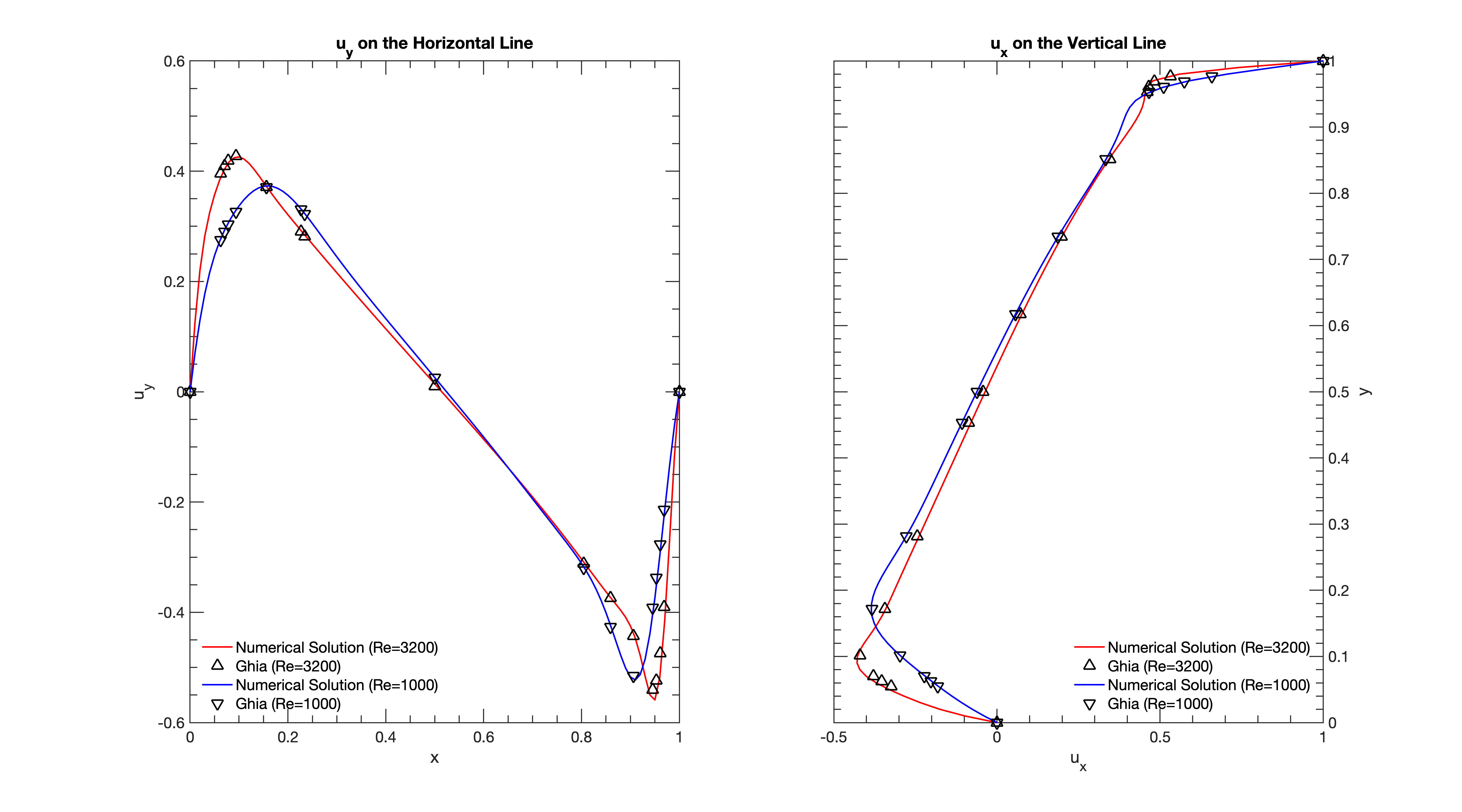
Figure 2: Benchmark Example 1. Velocity on the reference lines for $Re=1000$ (blue solid line) and $Re=3200$ (red solid line): (left) $u_{y}$ on the horizontal line and (right) $u_{x}$ on the vertical line. Numerical results are compared with the solutions from [40].

4.3 Model comparisons and parameter study

In this section, we perform several numerical tests for comparison study between the models of linearized Brinkman (6), Darcy-Brinkman (7), and Darcy-Brinkman-Forchheimer (3a). Particularly for parameter study, the role of Forchheimer term in (3a) is highlighted. Furthermore, the Navier-Stokes model is also compared if necessary. Henceforth, these models may be abbreviated as the D-B (Darcy-Brinkman), D-B-F (Darcy-Brinkman-Forchheimer), and N-S (Navier-Stokes).

The computational domain and boundary conditions for the lid-driven cavity filled with porous medium are depicted in Figure 1. For the steady lid-driven cavity flow, we have the Dirichlet boundary conditions in the absence of any sliding factor on the top boundary ($\Gamma_{D_{T}}$), but we have $\mathbf{u}_{T}=(1,0)$ on $\Gamma_{D_{T}}$. For the rest boundaries, the same boundary conditions are applied as in Section 4.2, i.e., the homogeneous boundaries. Note that the dotted reference lines passing the center are for comparing the velocity as the benchmarking example in the previous section (see Figure 2); $u_{x}$ is monitored from the vertical red, while $u_{y}$ is monitored from the horizontal blue. The domain starts with total 5 refinements globally, and perform its refinement cycle using the Kelly error estimator upto the max refinement number, for which we set 4 in this study.

Regarding the properties of porous medium, we fix porosity constant as $\phi=1.0$. Although the porosity is a variable depending upon the fluid pressure or volumetric strain of porous medium, by setting it constant as unity for simple analysis, we can purely investigate numerical aspects of the model and perform comparison study between the models. In the same manner, with an assumption of isotropic medium, intrinsic permeability ($K$) and inertial resistance ($\beta$) are taken as scalar coefficients instead of full tensor expressions. In order to test with the dimensionless parameters, i.e., $Re$ and $Da$ (see (4) and (5)) primarily, the reference (or the fundamental scale) parameters are set as Table 2, for which $\phi=1.0$ is presumed. Note that these reference values are problems- or environments-specific for porous medium, and they can be obtained from the experimental data such as the grain size and seepage rate from lab experiments. For the inertial resistance coefficient ($c_{F}$), it can be determined either empirically (from the relation of permeability) or theoretically (such as using Ergun’s equation [47]). In this numerical study, we fix it as $0.5$ for our reference value, unless otherwise noted.

Table 2: Scale parameters and inertial resistance coefficient that are selected in this study.

Parameter	Value	Unit
Reference distance ($L$)	$0.001$	$m$
Reference discharge ($U_{0}$)	$0.1$	$m/s$
Inertial resistance ($c_{F}$)	0.5	–

For the parameter study, three different values of Reynolds number are selected, i.e., $Re=10,100,$ and $1000$. Following a typical classification of the flow regime in porous media [79], the selected $Re$ values covers the laminar ($Re\leq 10$), the transient (or the nonlinear laminar, $10<Re\leq 100$), and the turbulent ($100<Re\leq 1000$) flow regimes. On the other hand, the intrinsic permeability $(K)$ is set with next six values: $2.5e$-$12$, $2.5e$-$11$, $2.5e$-$10$, $2.5e$-$7$, $2.5e$-$6$, and $2.5e$-$5$, with the unit of $m^{2}$. The former three can be categorized as relatively low permeability group compared to the latter three of relatively high permeability group. Using (5) with Table 2, $Da$ can then be obtained. With the combinations of these $Re$ and $Da$ numbers, there are 18 cases in total (see Table 3). For comparison purposes in this study, we categorize $Re\times Da$ values into two groups: GROUP I and GROUP II with nine cases for each. We note GROUP I is for $Re\times Da<1.0$ and GROUP II is for $Re\times Da\geq 1.0$. Accordingly, each $Re$ number owns six cases in total, where each group owns three examples. In Table 3, we denote the numbers for Test corresponding to cases in each group, following the order of $Re\times Da$ values from small to large.

Table 3: Numerical tests based on the values of $Re$ and $Da$ values. The left three columns of $Da$ belong to GROUP I, i.e., $Re\times Da$ $(<1.0)$, while the right three of it belong to GROUP II, $Re\times Da$ $(>1.0)$.

$Re\times Da$		$Da$
		2.5e-6	2.5e-5	2.5e-4	2.5e-1	2.5e+0	2.5e+1
$Re$	$10.0$	Test 1	Test 2	Test 3	Test 1	Test 2	Test 3
		2.5e-5	2.5e-4	2.5e-3	2.5e+0	2.5e+1	2.5e+2
	$100.0$	Test 4	Test 5	Test 6	Test 4	Test 5	Test 6
		2.5e-4	2.5e-3	2.5e-2	2.5e+1	2.5e+2	2.5e+3
	$1000.0$	Test 7	Test 8	Test 9	Test 7	Test 8	Test 9
		2.5e-3	2.5e-2	2.5e-1	2.5e+2	2.5e+3	2.5e+4

4.3.1 GROUP I: $Re\times Da<1.0$

As seen in Figure 3, Test 1, 5, and 9 are selected for succinct demonstration. The (left) column ((a), (d), (g)) is for the linearized Brinkman model, the middle column ((b), (e), (h)) is for the Darcy-Brinkman model and the (right) column ((c), (f), (i)) is for the full nonlinear Darcy-Brinkman-Forchheimer model. The cross mark in red and yellow is located at the exact location, the center of each domain. The three models are far from the Navier-Stokes model for the values of Reynolds number. This is due to the small $Da$ values resulting in $Re\times Da<1.0$ and higher viscous resistance. Regarding (b) $\dfrac{1}{ReDa}$ in Equation (3a) for Test 1, 5, and 9, their values are $40000$, $400$, and $4$, respectively. In the case of the full D-B-F model, higher inertial resistance also works.

The overall shape of streamlines of the three models are very similar, but Test 9 exhibits a slight difference in the location of the center of the eddy between the models, implying that the differentiation between the models has started. Figure 4 confirms that a deviation can be found distinctively with $u_{y}$ in Test 9. Meanwhile, it is shown that the D-B and the Brinkman models are almost identical in their values for the center line velocities. It indicates that for $Da$ and $Re$ values of this range, the convection does not make much difference to the momentum balance compared to the inertial resistance from the Forchheimer term.

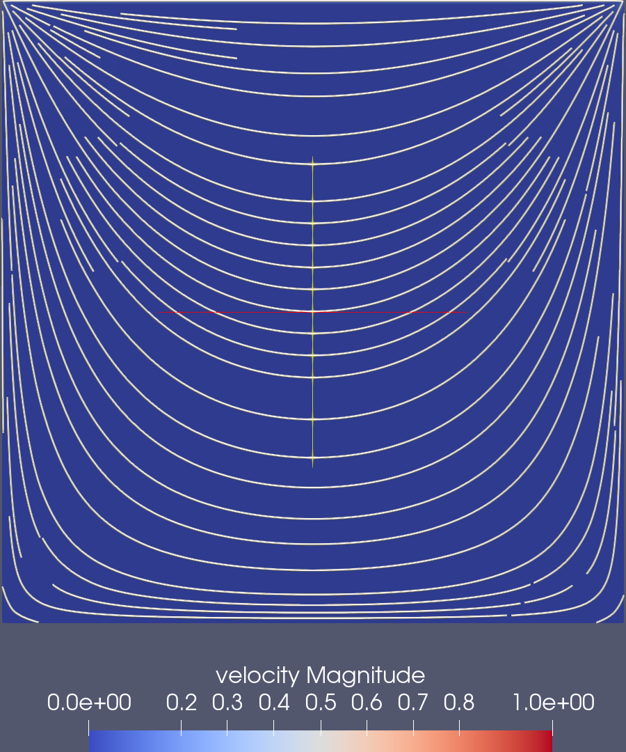
(a) Brinkman Test 1

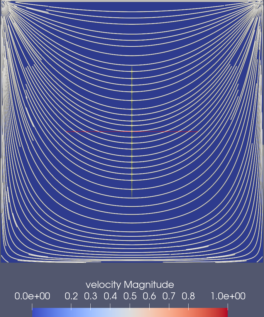
(b) D-B Test 1

(c) D-B-F Test 1

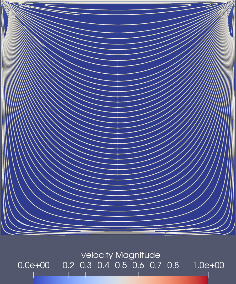
(d) Brinkman Test 5

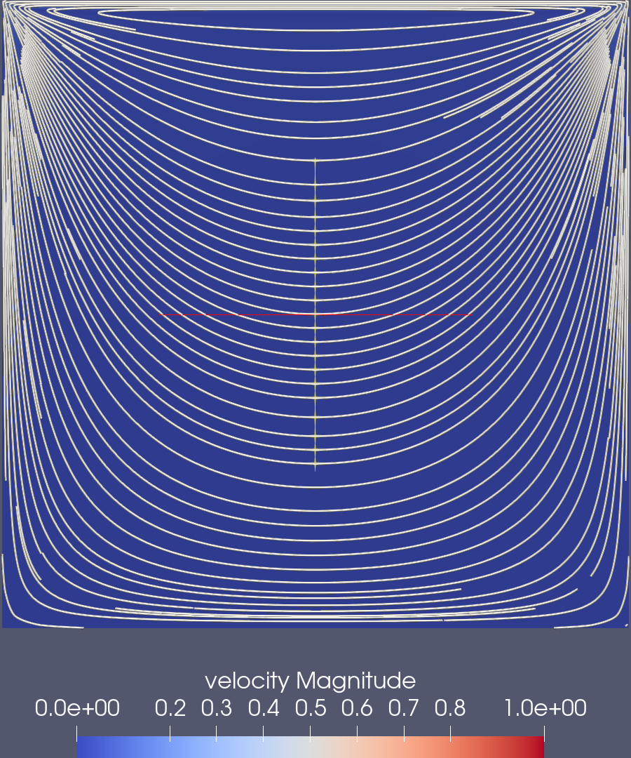
(e) D-B Test 5

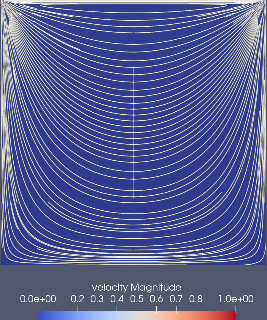
(f) D-B-F Test 5

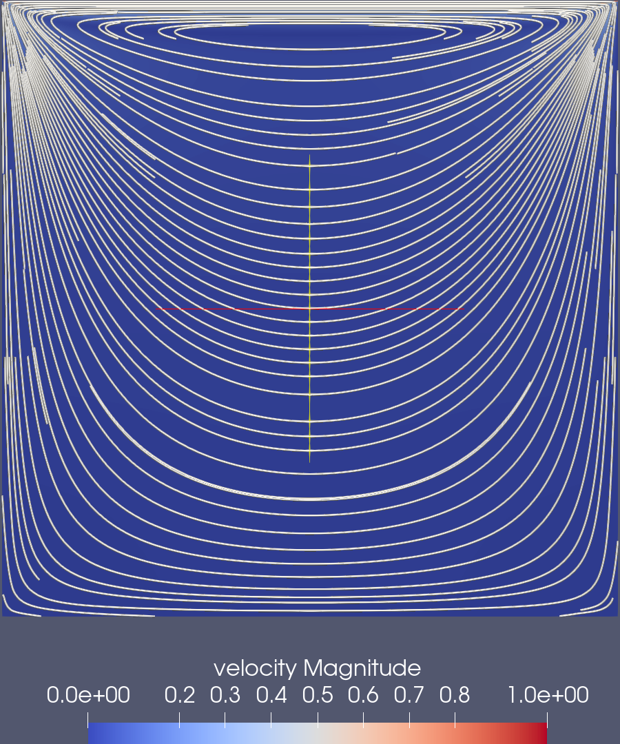
(g) Brinkman Test 9

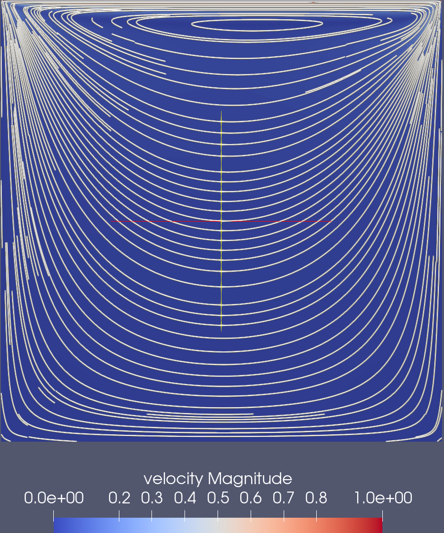
(h) D-B Test 9

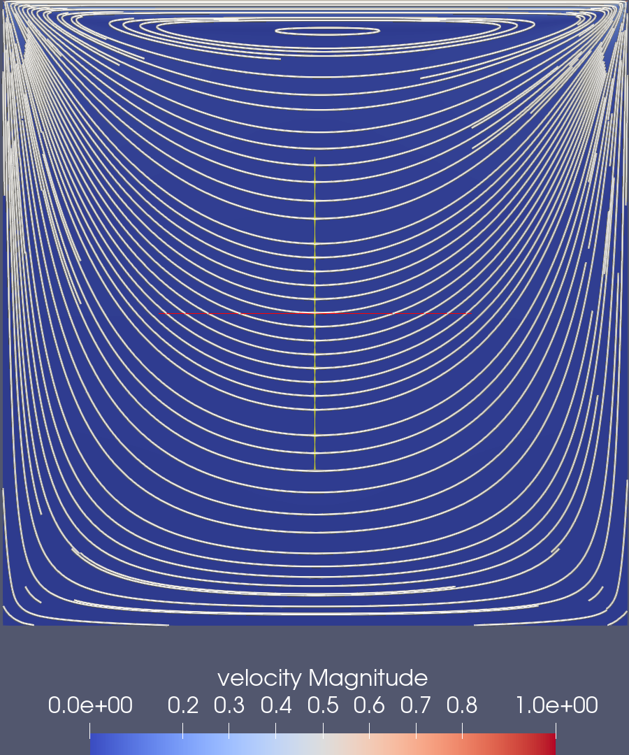
(i) D-B-F Test 9

Figure 3: [GROUP I] Test 1, 5, and 9. Velocity streamline: (left) Brinkman, (center) Darcy-Brinkman, and (right) Darcy-Brinkman-Forchheimer. Test 1, 5, and 9 have dimensionless numbers of 10, 100, 1000 for $Re$, and 2.5e-6, 2,5e-5, and 2.5e-4 for $Da$, respectively.

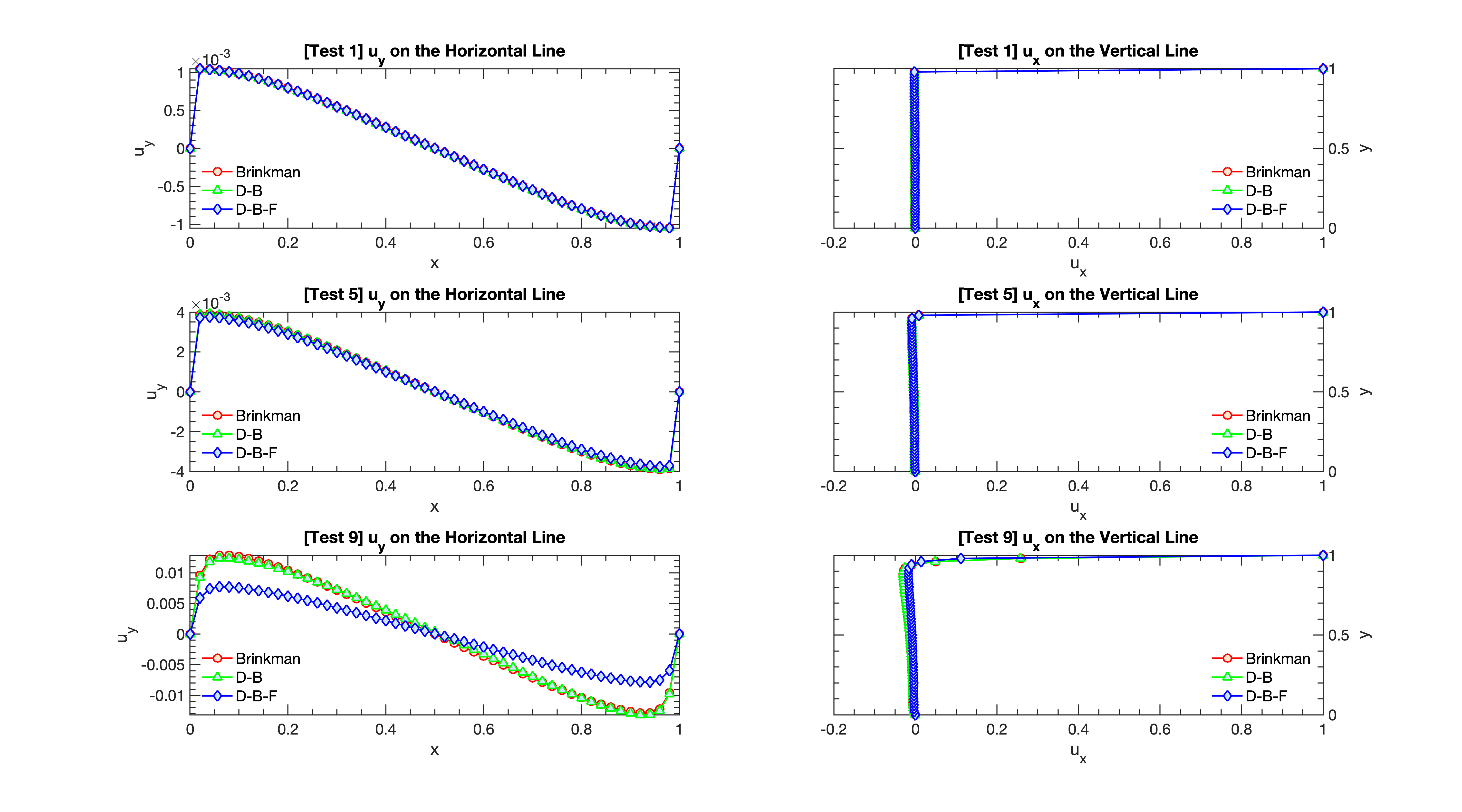
Figure 4: [GROUP I] Test 1, 5, and 9. Velocity on the reference lines using the Brinkman, Darcy-Brinkman, and Darcy-Brinkman-Forchheimer models. Test 1, 5, and 9 have dimensionless numbers of 10, 100, 1000 for $Re$, and 2.5e-6, 2,5e-5, and 2.5e-4 for $Da$, respectively.

Table 4 presents the outer Newton iteration numbers with flexible preconditioning iterative solver, FGMRES, in the last adaptive mesh refinement cycle (i.e., $4^{th}$) for each model for Test 1, 5, and 9. For both the D-B and D-B-F models, only one more iteration is added to the iteration number of the Brinkman model. Regarding the stabilization parameter for the Augmented Lagrangian term ((36) and (38)), we tested the numerics for the D-B-F model with $\gamma$ as $\gamma=0.0$. Although the specifics are omitted, we found that the iteration number for FGMRES has been severely increased with inefficiency.

On the other hand, Figure 5 illustrates the adaptive refinement using the Kelly error estimator on its last cycle for Test 9 with each model. The Brinkman model shows a nearly perfect symmetry due to the absence of the convection term, and the D-B model is the most asymmetric having the most nodes. For the full D-B-F model, it is alleviated by the inertial resistance by the Forchheimer term, which can be also found in Figure 3 from (g) to (i). Thus, it can be inferred that the convection term, still having a small impact, starts to reveal around the corner area compared to the center (see Figure 4). We also note that a naive Galerkin finite element method may produce oscillations and numerical instabilities near the corners due to the discontinuous property of the top boundary condition [56].

Table 4: [GROUP I] Total number of Newton iterations for Test 1, 5, and 9.

Test	Brinkman	D-B	D-B-F
Test 1	$3$	4	$4$
Test 5	$3$	4	$4$
Test 9	$3$	4	$4$

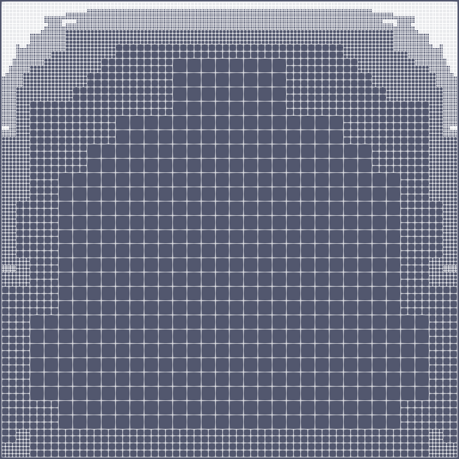
(a) Brinkman Test 9

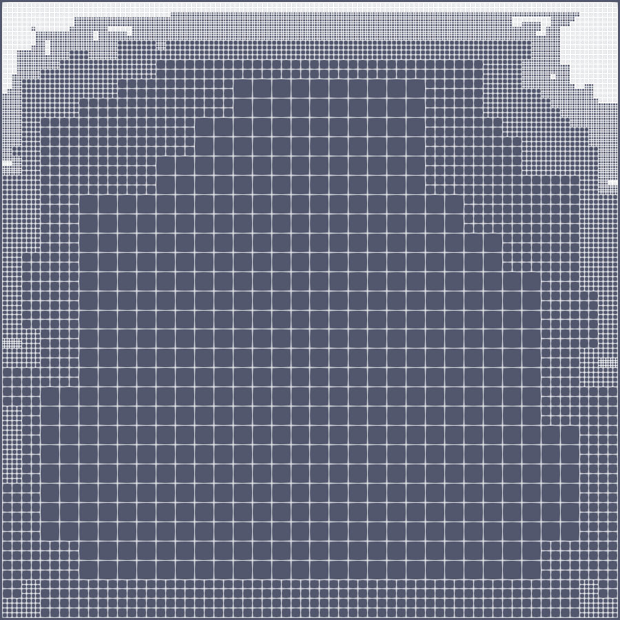
(b) D-B Test 9

(c) D-B-F Test 9

Figure 5: [GROUP I] Test 9. Adaptive mesh refinements of the last ($4^{th}$) cycle using the Kelly error estimator: (a) Brinkman, (b) Darcy-Brinkman, and (c) Darcy-Brinkman-Forchheimer. The total numbers of DoFs are (a) 154099 (DoFs for $\mathbf{u}_{h}$:136762, for $p_{h}$:17337), (b) 158253 (DoFs for $\mathbf{u}_{h}$:140454, for $p_{h}$:17799), (c) 144475 (DoFs for $\mathbf{u}_{h}$:128210, for $p_{h}$:16265).

In-depth study for GROUP I (with $Re$=10)

In this subsection, we investigate further about GROUP I with $Re$=10, and explore two other $Da$ values within $Re$=10.

$\bullet$ Test 2 & Test 3:

For in-depth study, we choose Test 2 and Test 3 and examine the Newton iterations of each model via probing numbers of FGMRES steps in each iteration. Both Test 2 & Test 3 have 3, 4, and 4 iterations in Newton for the Brinkman, D-B, and D-B-F models, respectively, the same as previous Tests in Table 4 at the last adaptive mesh refinement cycle, (i.e., $4^{th}$). However in Test 2, reaching the stopping criterion of $\varepsilon=1.0e$-$12$ takes the total FGRMES steps of 371, 449, and 435 for the Brinkman, D-B, and D-B-F models, respectively. For Test 3, corresponding numbers are 49, 77, 84. Overall, the Brinkman has quite less steps in FGMRES than others, while the D-B, and D-B-F models are close. Note also that Test 3 has much less numbers in those steps than those of Test 2, resulting from the Equation (41) as $Da$ number increases while $Re$ fixed as $Re=10$.

Table 5: [GROUP I] Number of FGMRES steps with Newton iterations for Test 2 and 3.

Test	Newton Iter.	Brinkman	D-B	D-B-F
Test 2	1	2	2	2
	2	130	118	118
	3	239	187	182
	4	-	142	133
Test 3	1	2	2	2
	2	20	19	19
	3	27	28	28
	4	-	28	35

$\bullet$ $Da=0.0025$ and $Da=0.025$:

As seen in Figure 4, a clear deviation of D-B-F model from two other models is found for the turbulent regime, i.e., $Re=1000$ (Test 9). We further test if any notable deviation starts while fixing $Re=10$. Since Test 2 and 3 does not show those deviations (not reported explicitly here), we test cases outside GROUP I (in between GROUP I and GROUP II) via increasing $Da$ values to $Da=0.0025$ and $Da=0.025$, while fixing $Re=10$.

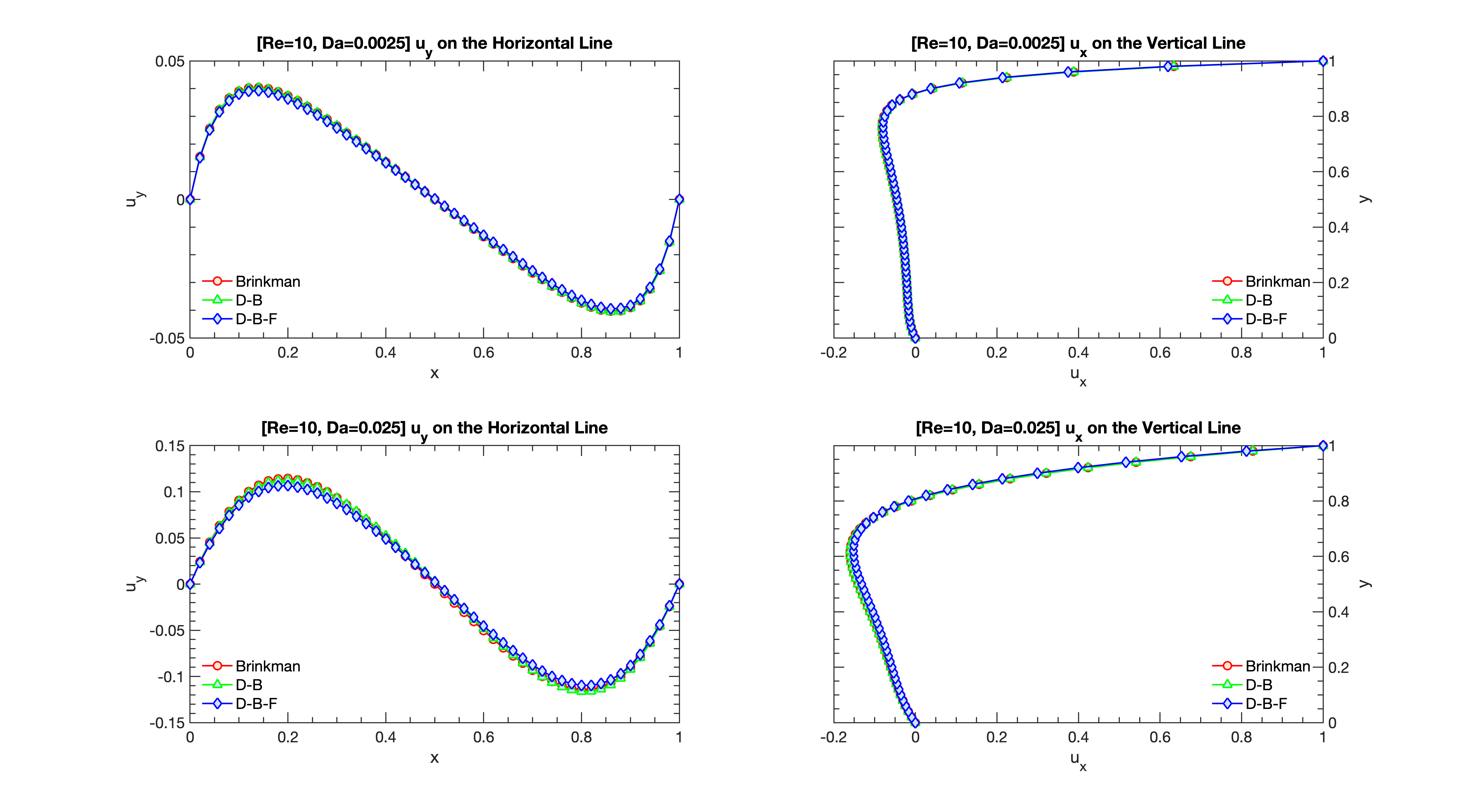
Figure 6: [$Re=10$] $Da=0.0025$ (first row) and $Da=0.025$ (second row). Velocity on the reference lines using the Brinkman, Darcy-Brinkman, and Darcy-Brinkman-Forchheimer models.

As demonstrated in Figure 6, we find a slight departure has started when $Da=0.0025$ and more in case of $Da=0.025$. Although $Da$ is not realistic nor any experimental, it seems a very tiny deviation, called weak inertia regime [43] exists for $Re=10$, which can be negligible from engineering perspective. Note also that Test 9 with $Re$ variation captures more deviations of D-B-F in $u_{y}$ than those in $u_{x}$. Unlike the case, $Da=0.025$ has similar deviations of D-B-F in $u_{x}$ and $u_{y}$, even though both Test 9 and $Da=0.025$ have the same $Re\times Da=0.25$. This is attributed to the property of $Re$, where the inverse of it implies the ratio of viscous force to inertial force (see Equation (4)). We will see similar trend can be found in the GROUP II Test 1. Remind that the D-B-F model is convergent to the N-S system when $Da$ goes to greater number, ultimately being identical if $Da\rightarrow\infty$.

4.3.2 GROUP II: $Re\times Da>1.0$

In this section, several tests are addressed for GROUP II having $Re\times Da>1.0$ and the Navier-Stokes model can also be compared with the three models if necessary. For brevity as well, Test 1, 5, and 9 are selected, Some other examples are left for in-depth study in the following subsection.

Unlike GROUP I, the secondary and tertiary vortices at the left and right bottom corner appear in GROUP II, showing the enhanced nonlinearity from increased of $Re\times Da$. As seen in Figure 7, both the D-B (center) and the full nonlinear D-B-F (right) models have departed from the Brinkman (left) model in overall shape of streamlines, except for Test 1 ((a), (b), (c) in Figure 7). It results from the relatively high viscous force working for Test 1, where similar phenomena can apply to other $Re=10$ cases, i.e., Test 2 and Test 3 as aforementioned in the previous section. As the flow regime changes from the laminar to the turbulent (from Test 1 to Test 9), we find that the center of primary eddy of D-B or D-B-F model migrates down toward the center cross due to the increased intensity of convection term, as GROUP II is under weaker viscous resistance unlike GROUP I. Meanwhile, without the convection term, those of the Brinkman stay at the same height on top of the vertical cross line at the center. The overall shape of the streamlines of the D-B and D-B-F models appear to be similar except for slight differences in the type and size of curves for the secondary and tertiary vortices at the bottom left and right corners. The size of vortices for D-B-F model is modestly smaller than those of D-B due to the inertial resistance, i.e., (c) $\dfrac{c_{F}}{\sqrt{Da}}$ in (3a).

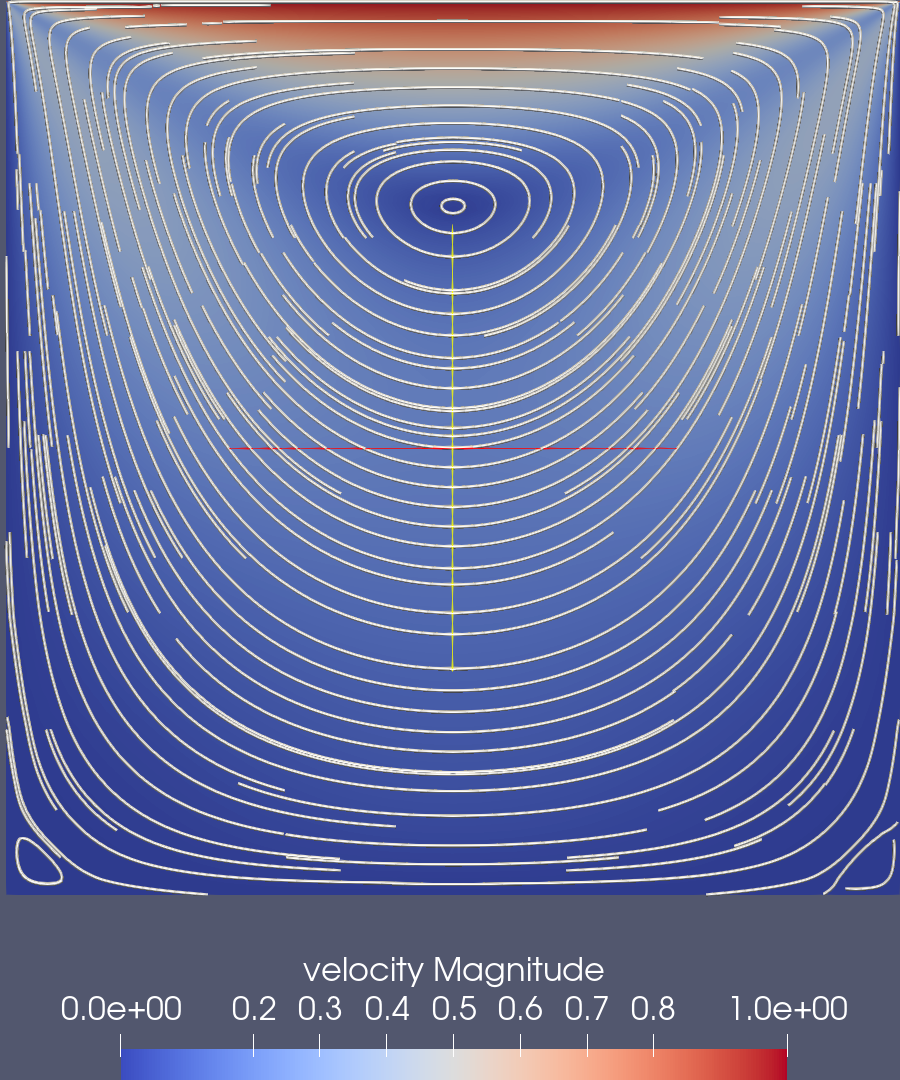
(a) Brinkman Test 1

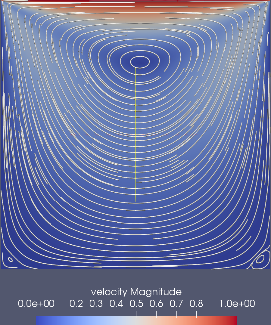
(b) D-B Test 1

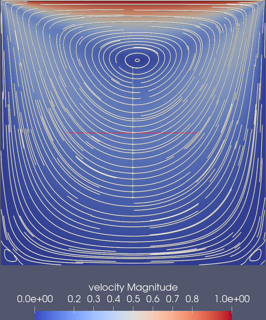
(c) D-B-F Test 1

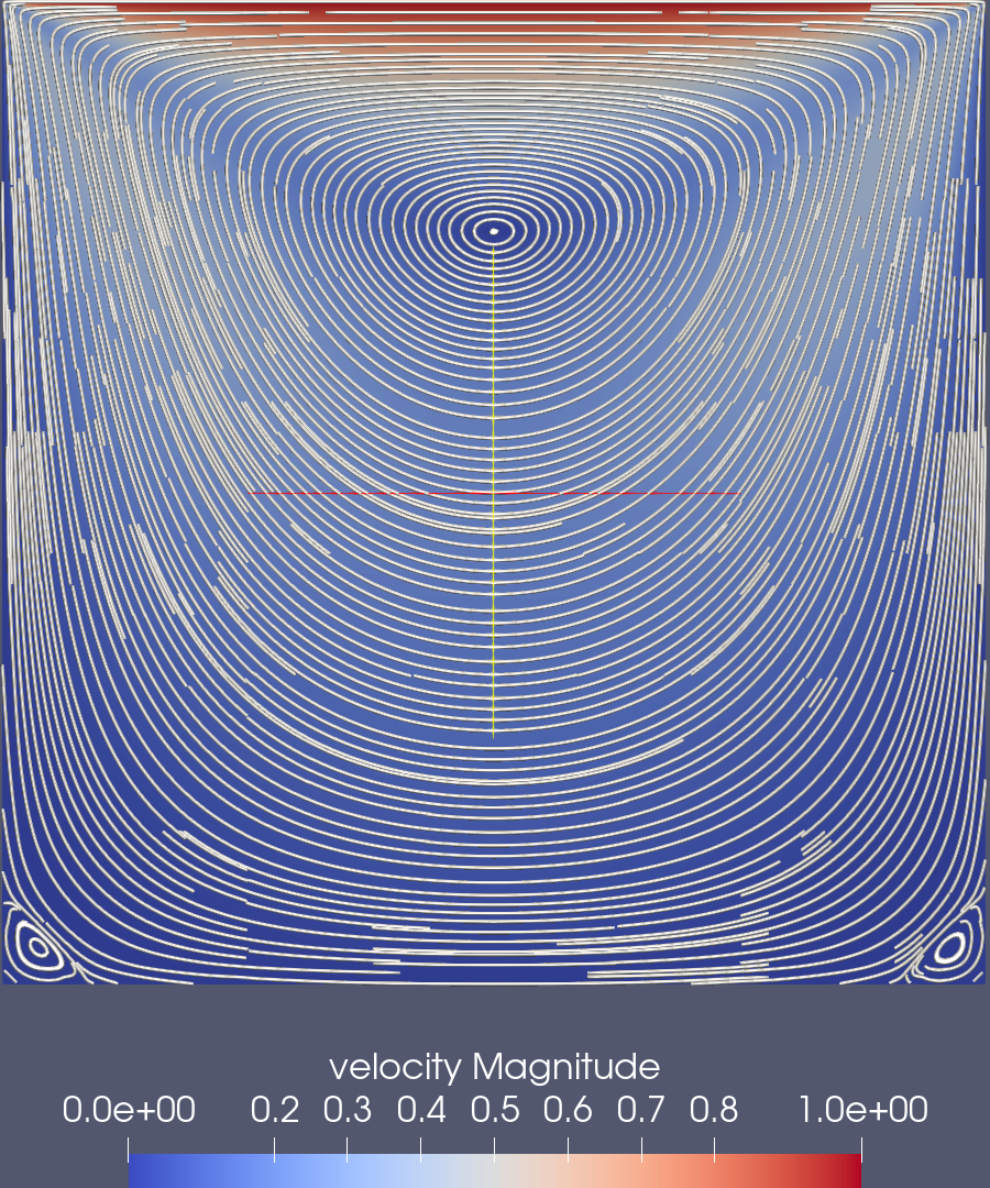
(d) Brinkman Test 5

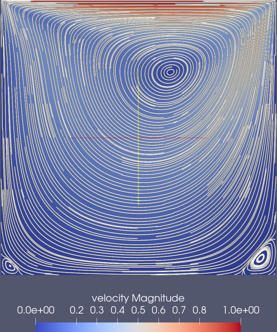
(e) D-B Test 5

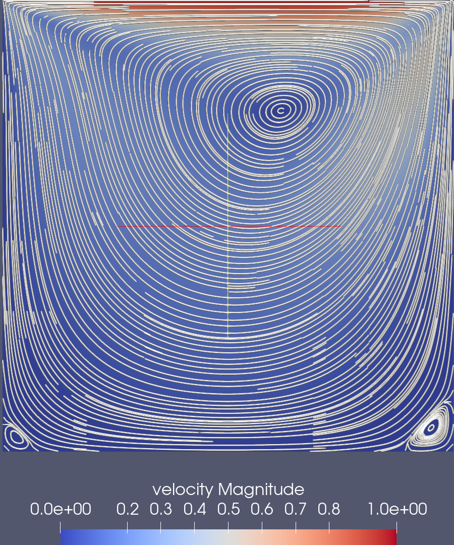
(f) D-B-F Test 5

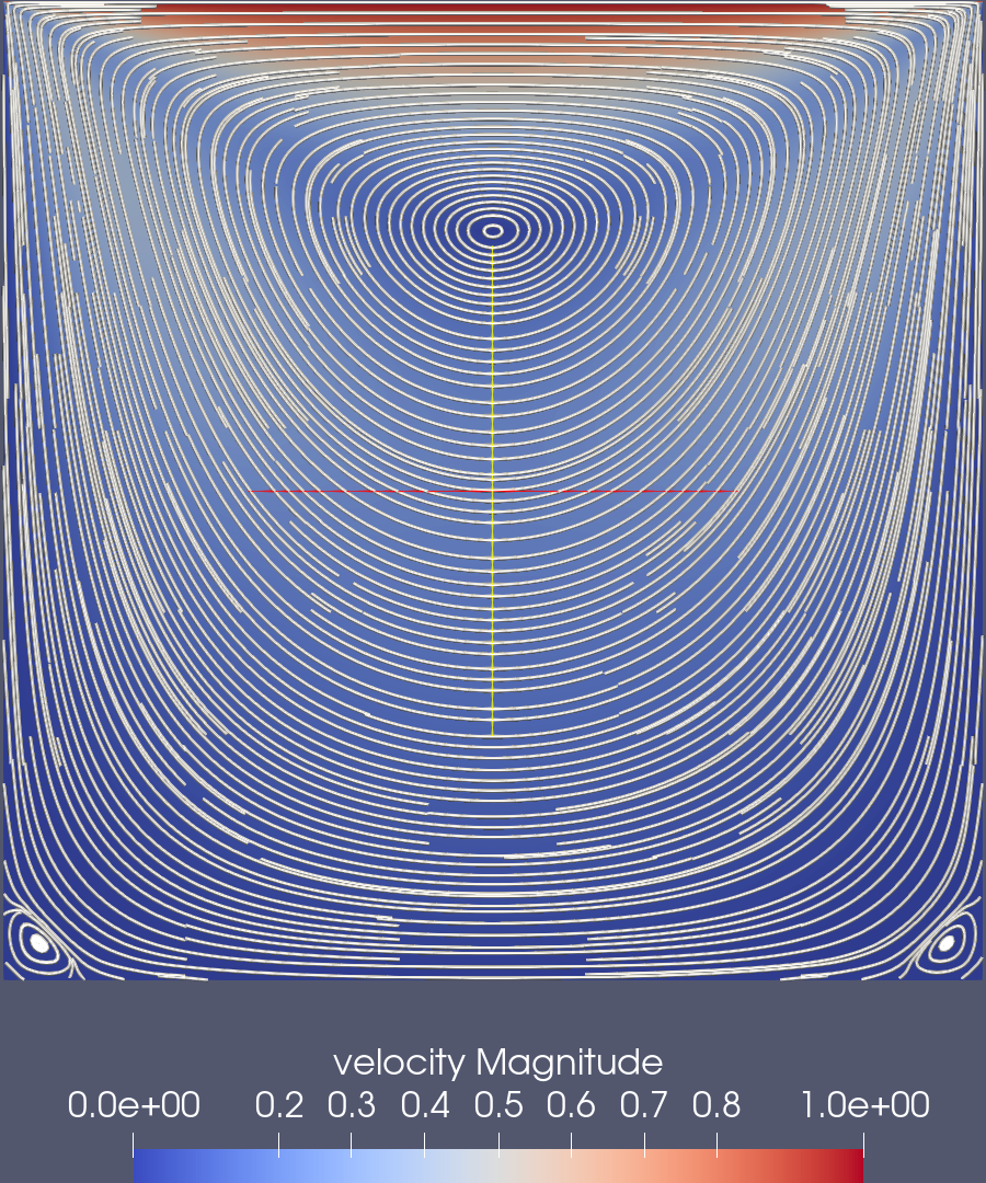
(g) Brinkman Test 9

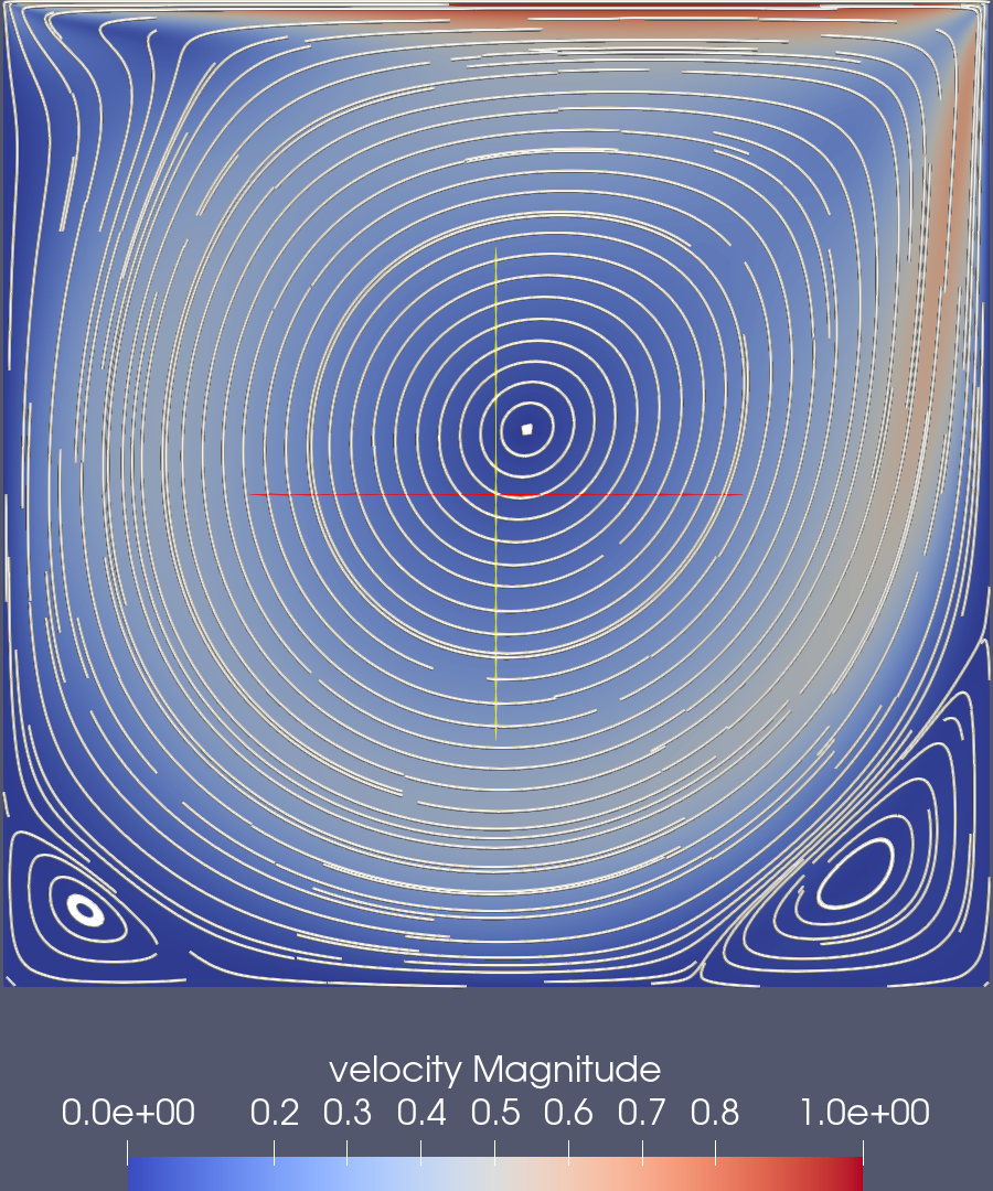
(h) D-B Test 9

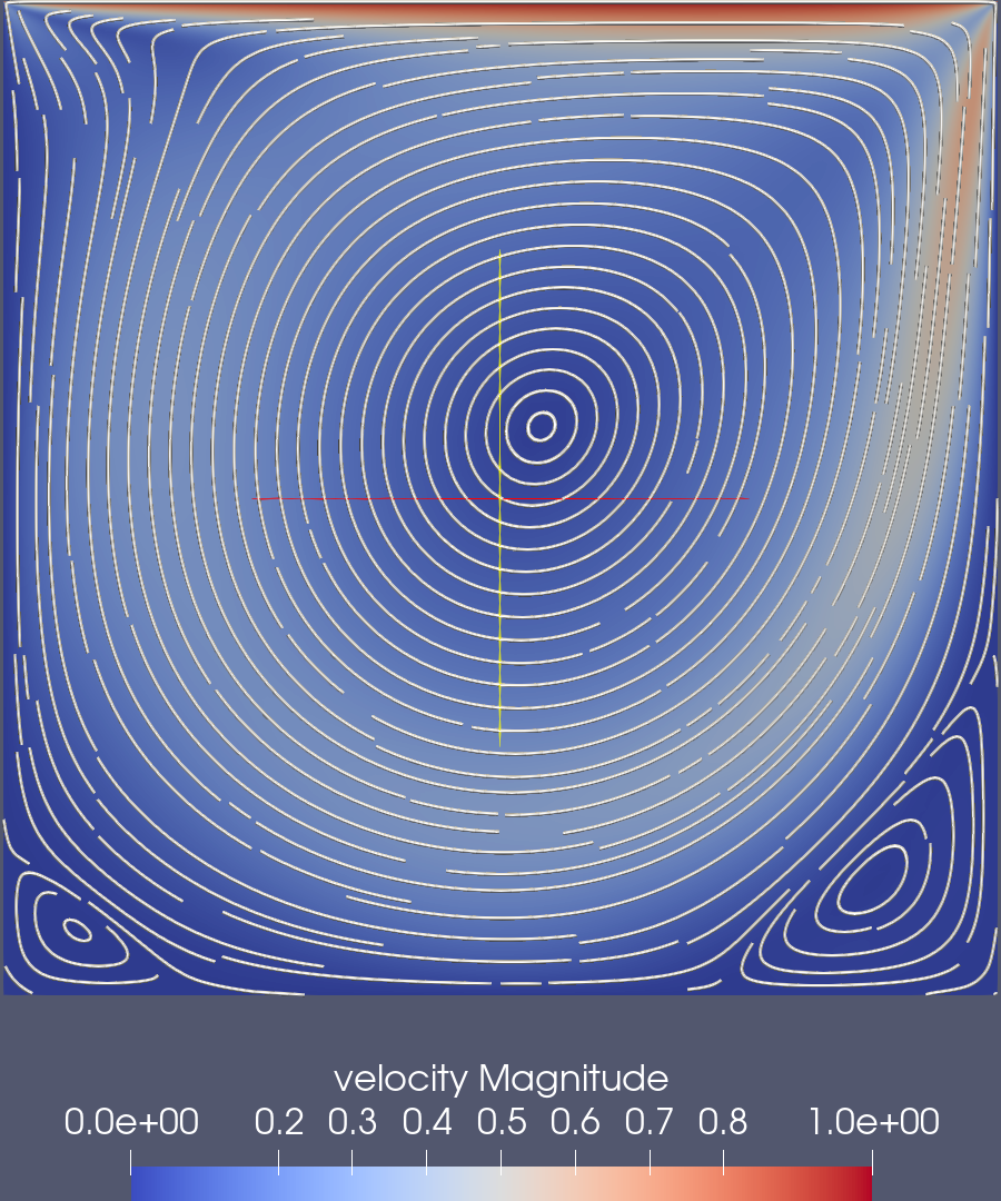
(i) D-B-F Test 9

Figure 7: [GROUP II] Test 1, 5, and 9. Velocity streamline: (left) Brinkman, (center) Darcy-Brinkman, and (right) Darcy-Brinkman-Forchheimer. Test 1, 5, and 9 have dimensionless numbers of 10, 100, 1000 for $Re$, and 2.5e-1, 2,5e+0, and 2.5e+1 for $Da$, respectively.

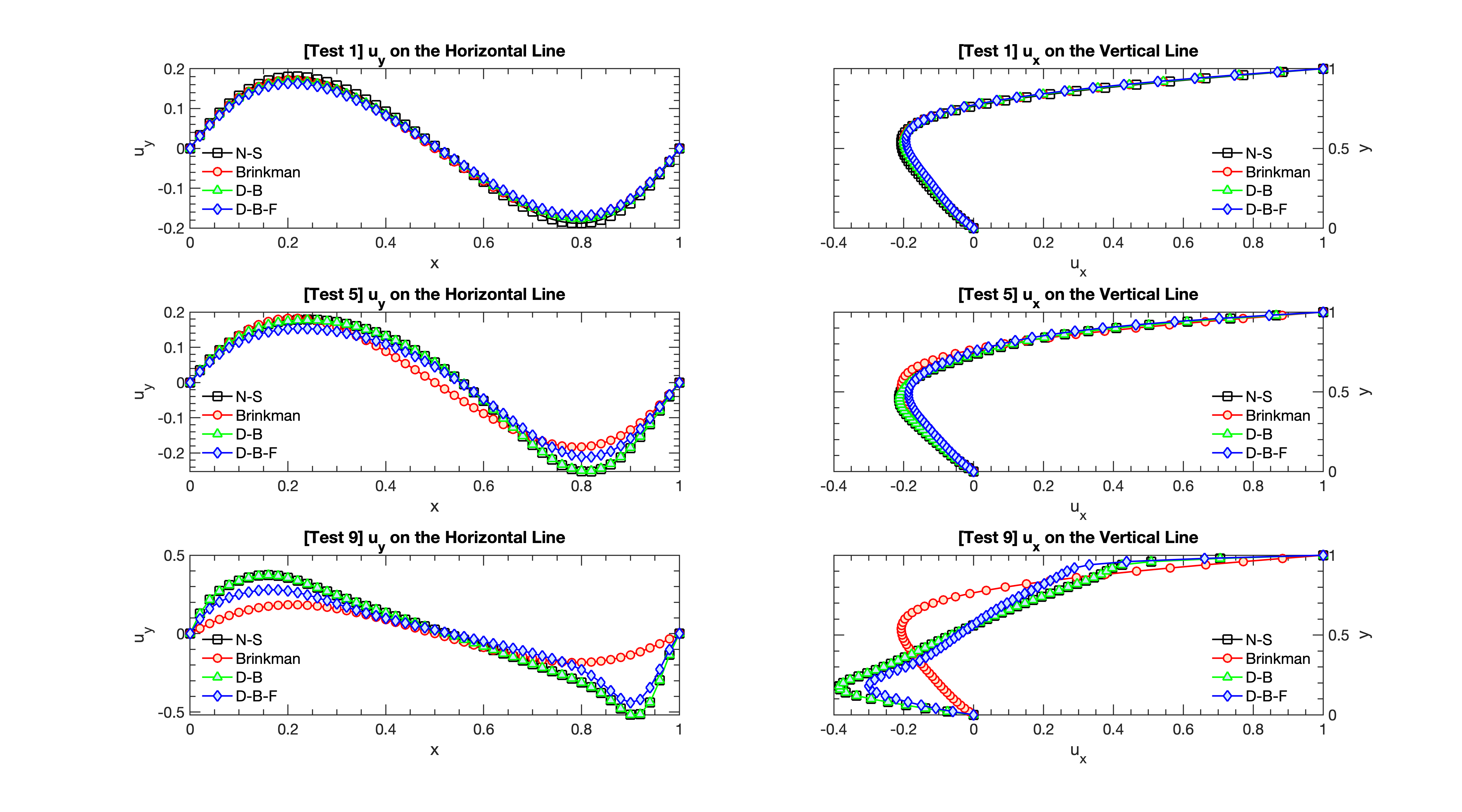
Figure 8: [GROUP II] Test 1, 5, and 9. Velocity on the reference lines using the Brinkman, Darcy-Brinkman, and Darcy-Brinkman-Forchheimer models, compared with the Navier-Stokes model. Test 1, 5, and 9 have dimensionless numbers of 10, 100, 1000 for $Re$, and 2.5e-1, 2,5e+0, and 2.5e+1 for $Da$, respectively.

The velocity profiles on the reference lines (Figure 8) present more distinctiveness between the models. Regarding $u_{y}$ profiles on the horizontal reference line ((left) of Figure 8), the D-B, D-B-F, and N-S models become more asymmetric compared to more symmetric Brinkman model with increasing values of $Re\times Da$. More importantly, unlike GROUP I where the D-B is overlapping the Brinkman, here the D-B is almost identical to the N-S for three Tests. As a homogenized model from the N-S [44], the D-B model is the case when $c_{F}=0$ in (c) $\dfrac{c_{F}}{\sqrt{Da}}$. Still, the D-B-F is differentiated from the D-B and N-S models, not to mention the Brinkman model. Through the last mesh refinements of Test 9 (see Figure 9), we confirm the Brinkman demonstrates the symmetry, and there are notable deviations between the three models: the Brinkman, D-B and D-B-F. We also identify that the maximum adaptive grid refinements occur locally near the top boundary where the discontinuity condition is applied. As similar to GROUP I, the D-B model has the most nodes with DoFs.

(a) Brinkman Test 9

(b) D-B Test 9

(c) D-B-F Test 9

Figure 9: [GROUP II] Test 9. Adaptive mesh refinements of the last ($4^{th}$) cycle using the Kelly error estimator: (a) Brinkman, (b) Darcy-Brinkman, and (c) Darcy-Brinkman-Forchheimer. The total numbers of DoFs are (a) 175303 (DoFs for $\mathbf{u}_{h}$:155674, for $p_{h}$:19629), (b) 229747 (DoFs for $\mathbf{u}_{h}$:204006, for $p_{h}$:25741), (c) 215585 (DoFs for $\mathbf{u}_{h}$:191430, for $p_{h}$:24155).

Table 6 shows the Newton iteration numbers, which are identical to the ones in GROUP I. Unlike GROUP I, when the Augmented Lagrangian term is set with $\gamma=0.0$ for the D-B-F model, the iterative solver of FGMRES fails to converge. This implies that the increased nonlinearity requires the balanced Augmented Lagrangian term, and an appropriate value of $\gamma$ must be provided.

Table 6: [GROUP II] Total number of Newton iterations for Test 1, 5, and 9.

Test	Brinkman	D-B	D-B-F
Test 1	$3$	4	$4$
Test 5	$3$	4	$4$
Test 9	$3$	4	$4$

In-depth study for GROUP II

In this subsection, the remaining Tests in GROUP II are investigated with in-depth study on the departure of the full Darcy-Brinkman-Forchheimer model from other models, including the Navier-Stokes, highlighting the Forchheimer term for inertial resistance.

$\bullet$ Test 4 & Test 6:

Test 4 and Test 6 are in the transient regime for the porous medium with fixed $Re=100$. As can be seen in Figure 10, particularly from the Brinkman model, the increased $Da$ intensifies the vorticity, which can be found in other models as well. Test 4 has a slight more difference in the location of primary eddy between the D-B and the D-B-F models (see (b) and (c) in Figure 10) than the that of Test 6 (see (e) and (f) in Figure 10), exhibiting more effect of inertial resistance compared to the viscous resistance, which is via the Forchheimer term.

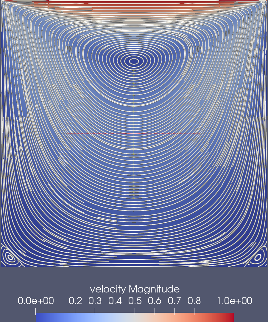
(a) Brinkman Test 4

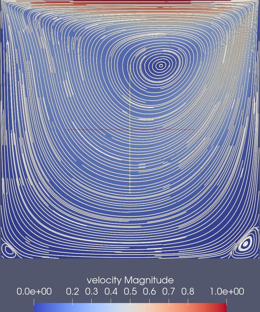
(b) D-B Test 4

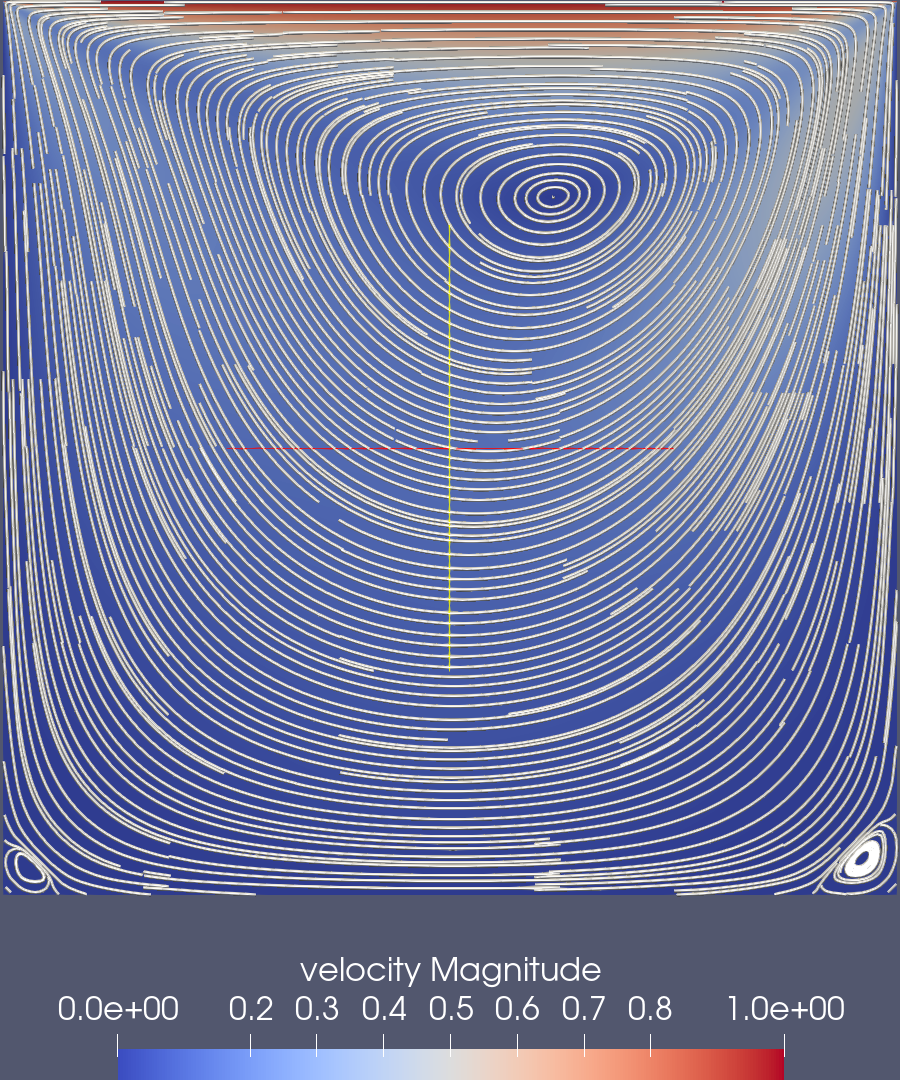
(c) D-B-F Test 4

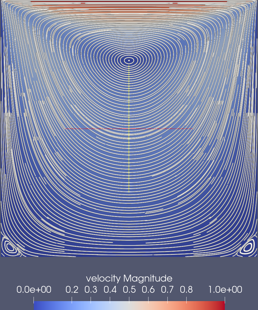
(d) Brinkman Test 6

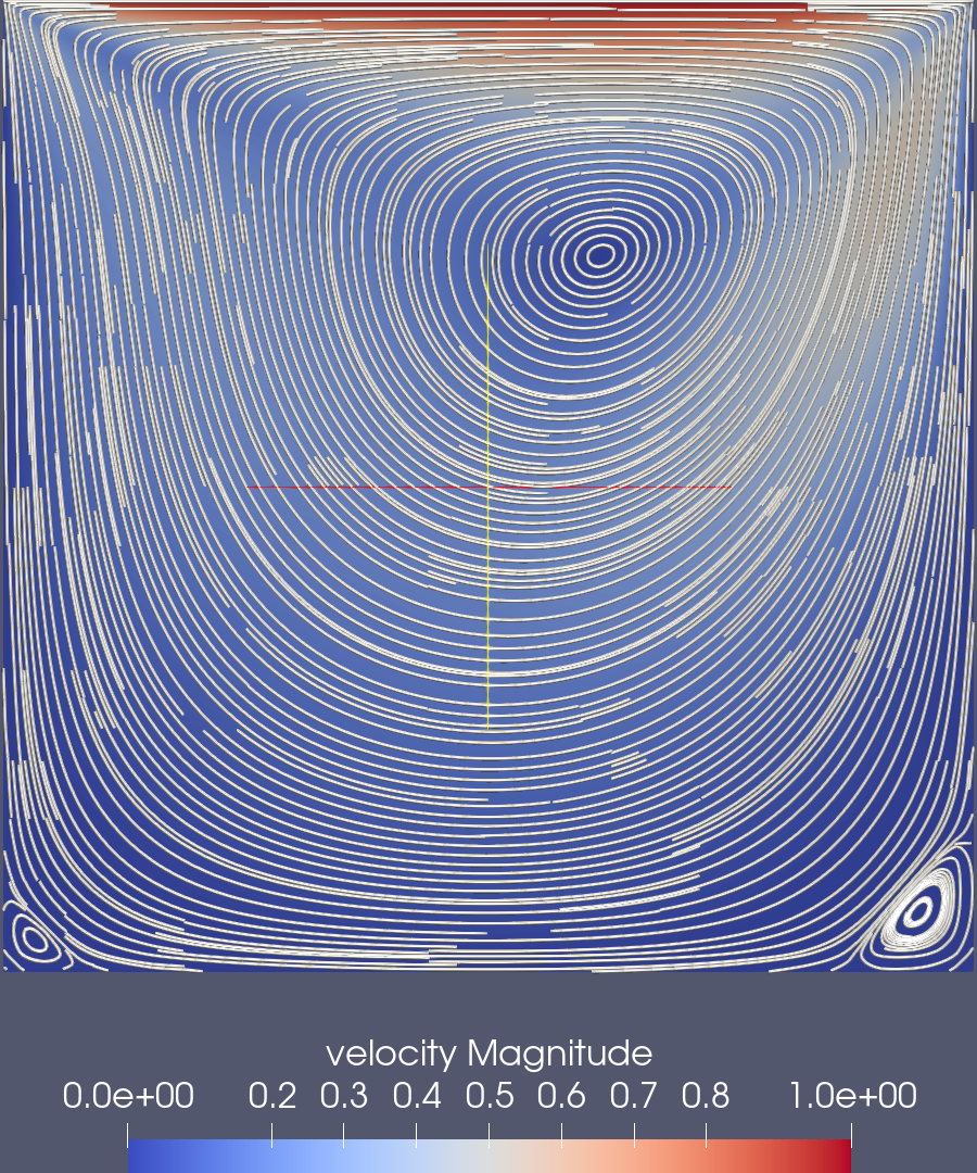
(e) D-B Test 6

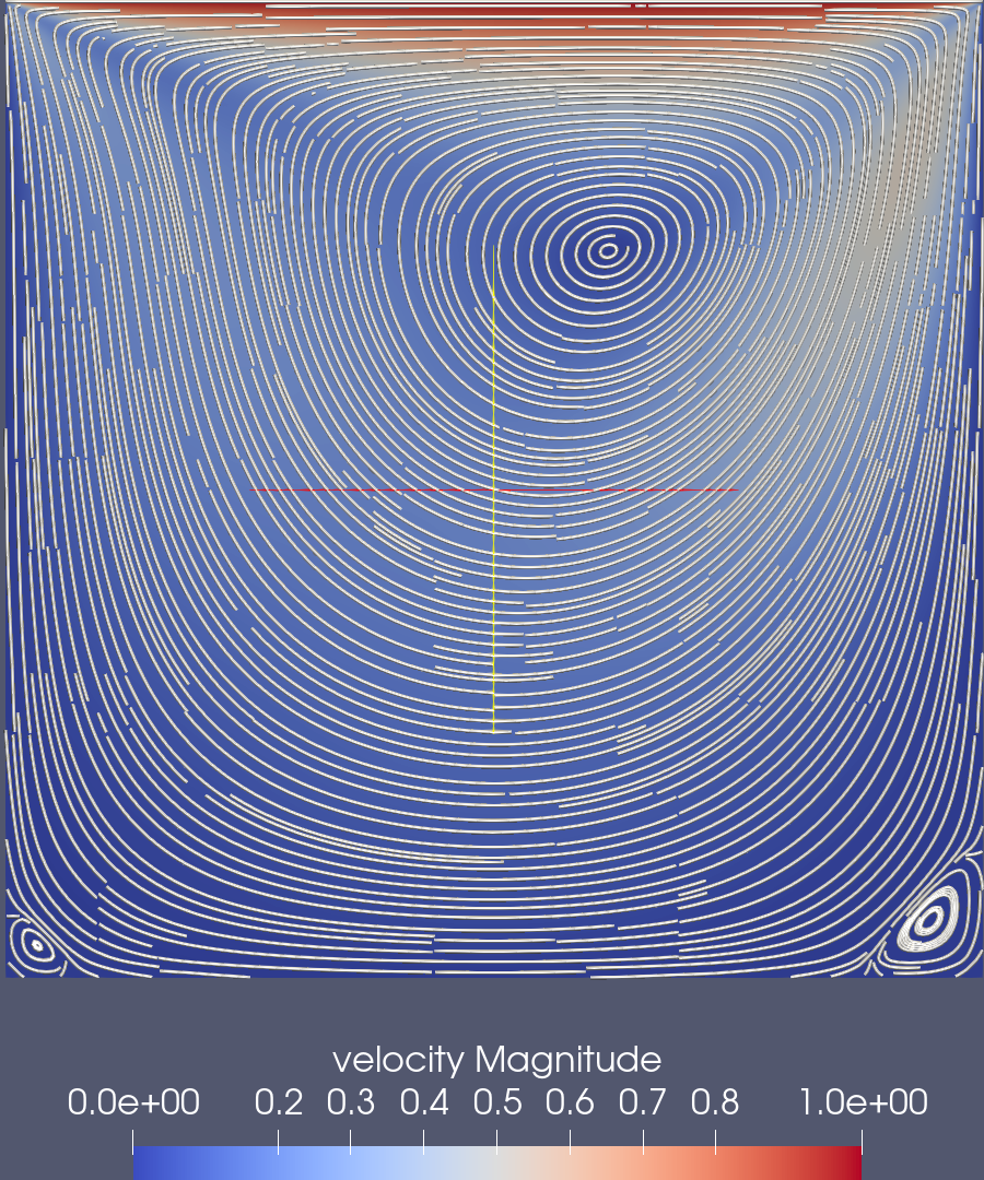
(f) D-B-F Test 6

Figure 10: [GROUP II] Test 4 and 6. Velocity streamline: (left) Brinkman, (center) Darcy-Brinkman, and (right) Darcy-Brinkman-Forchheimer. Test 4 and 6 have dimensionless numbers of 100 for $Re$ and 2.5e-1 and 2.5e+1 for $Da$, respectively.

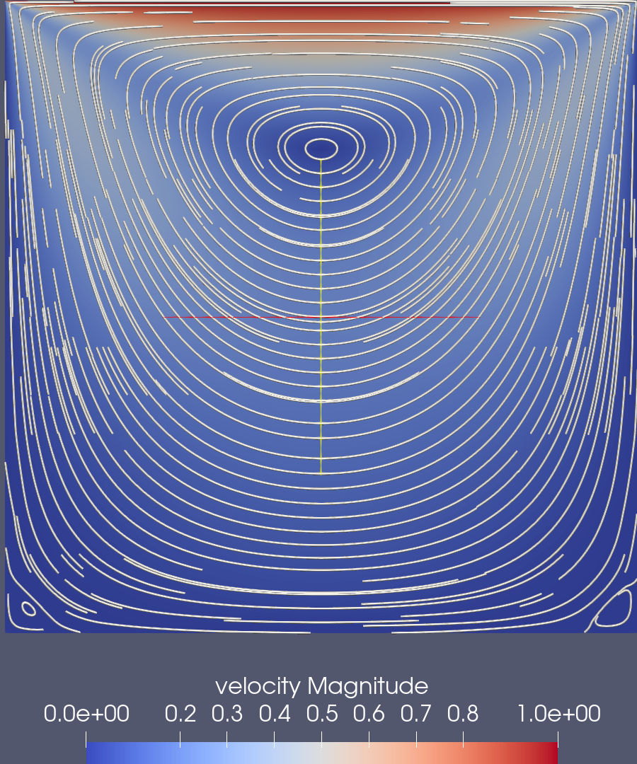
(a) Brinkman Test 2

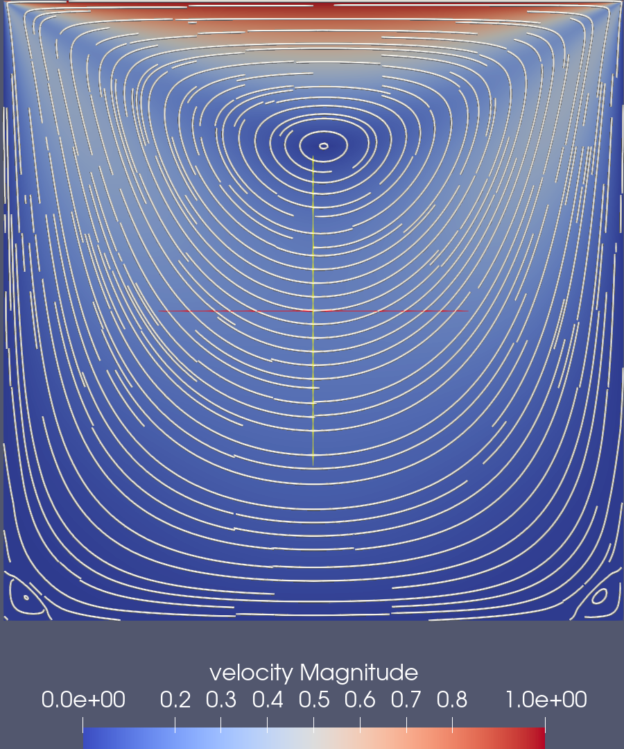
(b) D-B Test 2

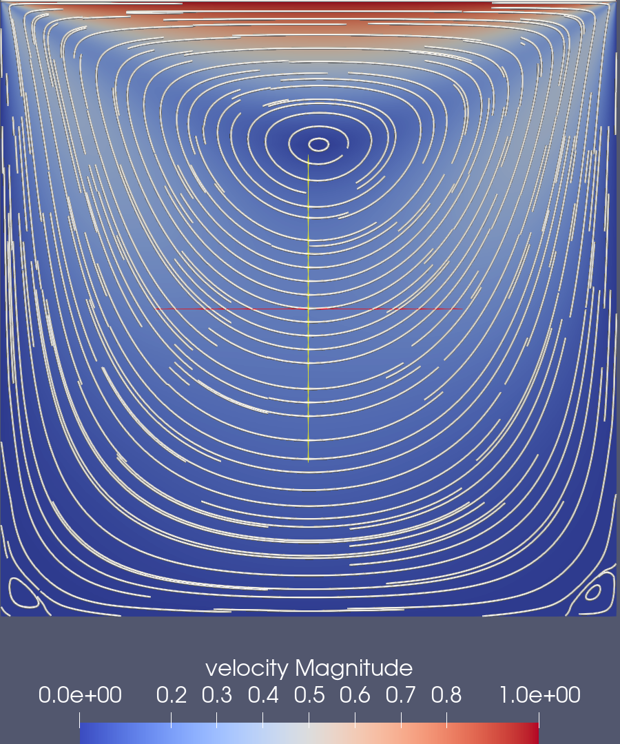
(c) D-B-F Test 2

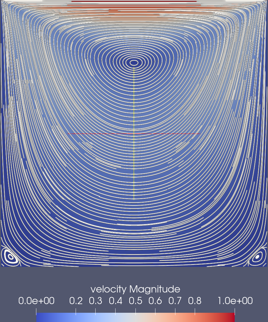
(d) Brinkman Test 8

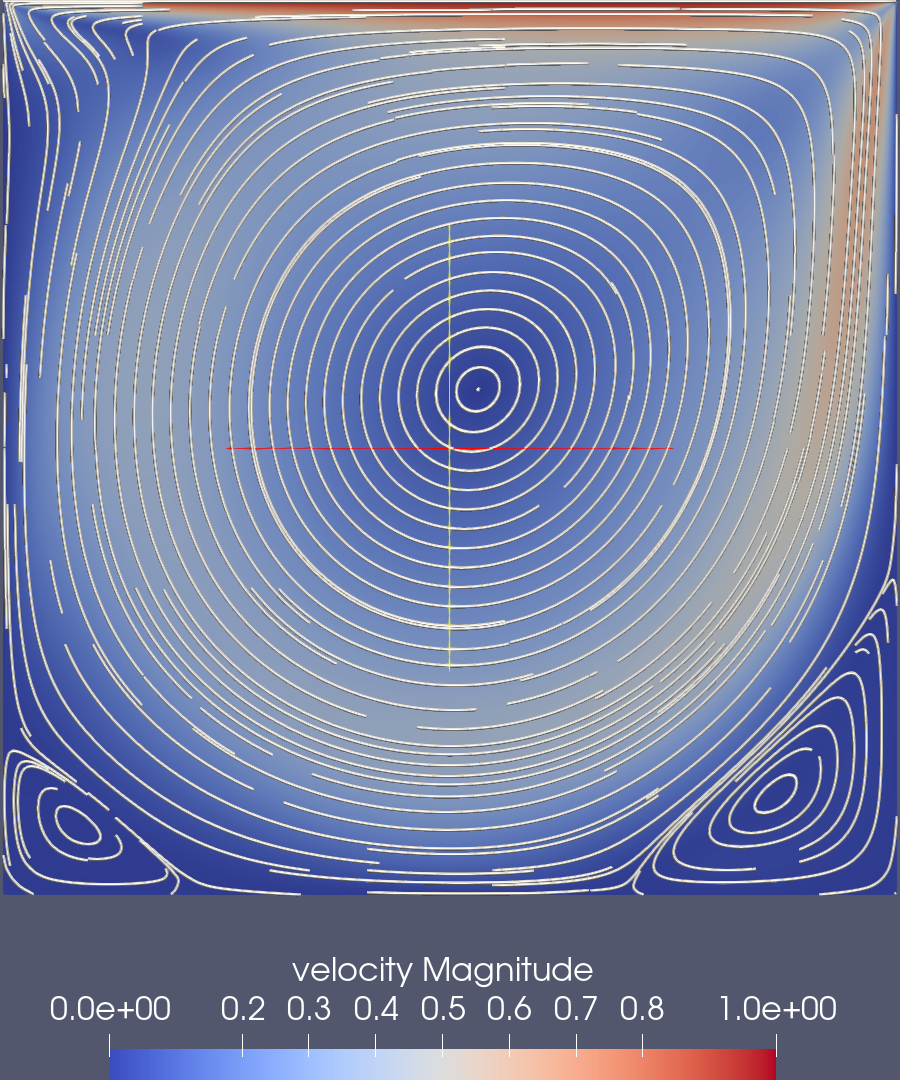
(e) D-B Test 8

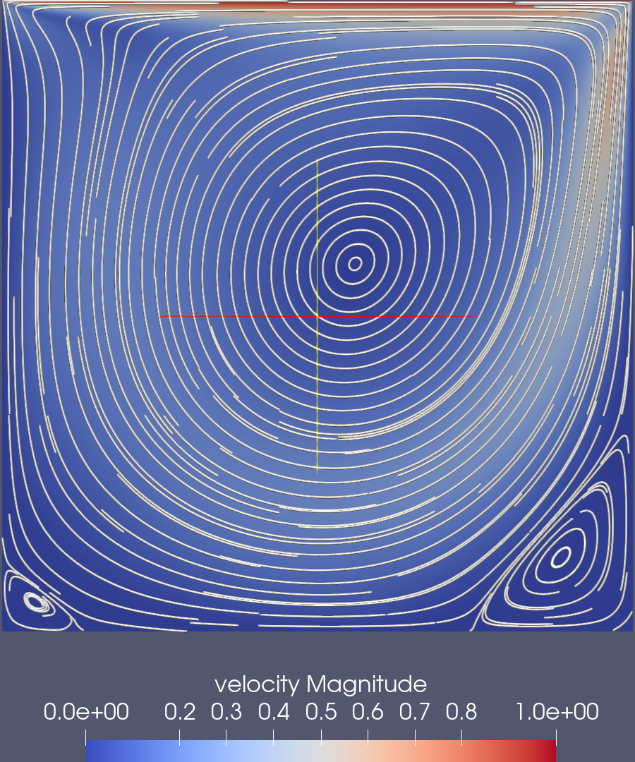
(f) D-B-F Test 8

Figure 11: [GROUP II] Test 2 and 8. Velocity streamline: (left) Brinkman, (center) Darcy-Brinkman, and (right) Darcy-Brinkman-Forchheimer. Test 2 and 8 have dimensionless numbers of 10 and 1000 for $Re$, respectively, and 2.5e+0 for $Da$.

$\bullet$ Test 2 & Test 8:

From Test 2 and Test 8, we identify that $Re$ variation with fixed $Da$ has more effects on the flow than $Da$ variation with fixed $Re$ does (see Figure 11 compared to Figure 10). Much difference in streamlines between examples, i.e., Test 2 and Test 8 within each model, is due to different $Re$ values, resulting in the change of flow regimes; Test 2 is in the laminar, whereas Test 8 is in the turbulence for a typical porous medium. Albeit the same increasing ratio of $100$ applied for $Re$ as for $Da$ in the previous case (see Table 3), we find that $Re$ that has more influence (see (3a)) for this lid-driven cavity problem under the unit velocity (i.e., the maximum velocity), implying that the flow regime change is more abrupt and instantaneous [79].

Note also that when the intensity of vorticity is increased by either $Da$ or $Re$, the growth of vortices is somewhat restricted for the D-B-F model compared to the D-B model, where the only difference is the existence of inertial resistance. As seen in Figure 10 and 11, the size of vortices from the D-B-F is smaller than those from the D-B, which is distinctively shown in the turbulent regime.

$\bullet$ Test 7:

Test 7 is selected to investigate further the effect of the inertial resistance to the flow. Note that the ratio of (c) $\dfrac{c_{F}}{\sqrt{Da}}$ in (3a) compared to $Re$, i.e., the value of $\dfrac{c_{F}}{\sqrt{Da}}$, Test 7 has the largest for all Tests in GROUP I and GROUP II (see Table 3). In addition, the distance from the Navier-Stokes system, i.e., $Da\rightarrow\infty$, in terms of (b) $\dfrac{1}{ReDa}$ and (c) $\dfrac{c_{F}}{\sqrt{Da}}$ in (3a), Test 7 is the farthest among all Tests in GROUP II.

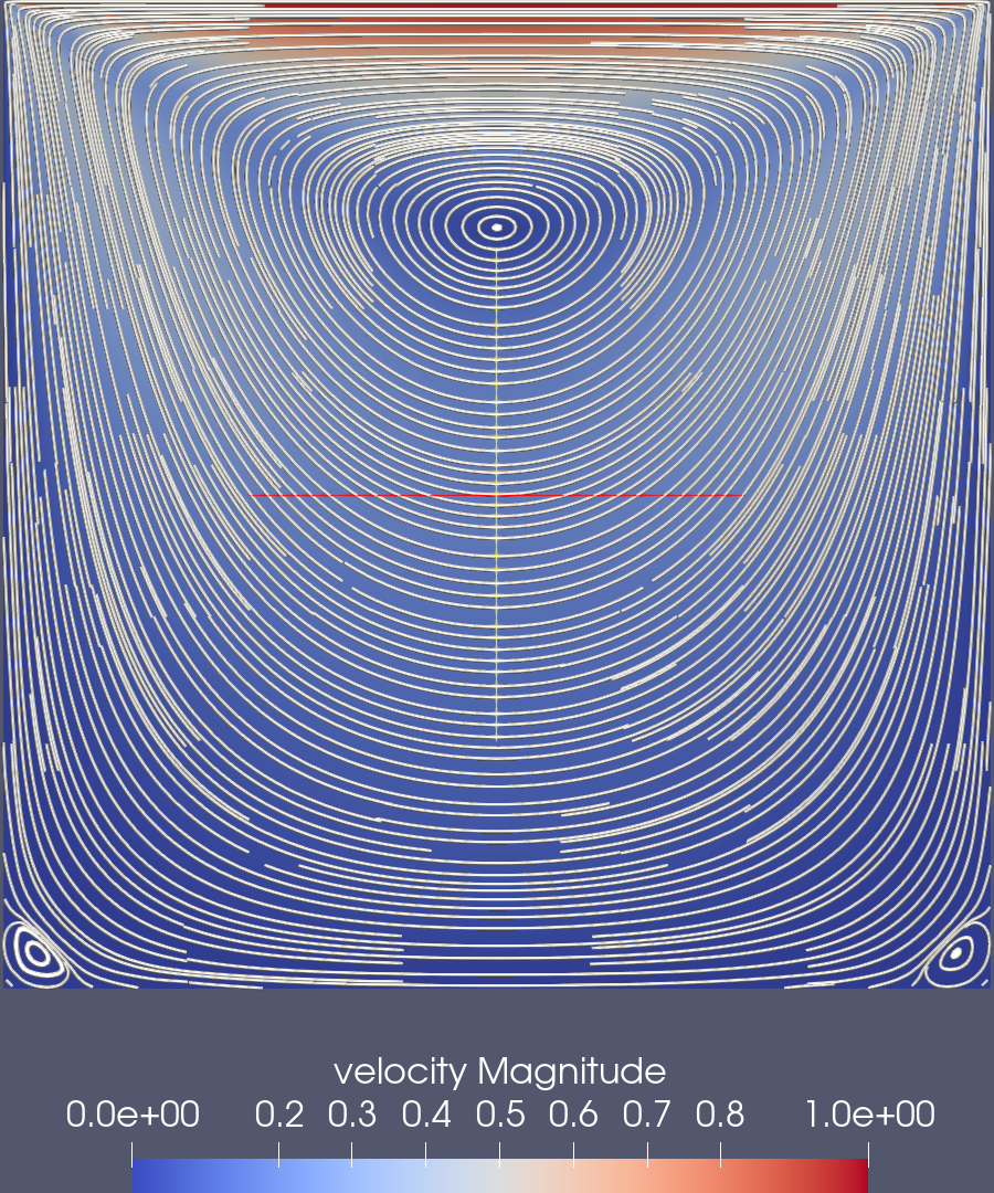
(a) Brinkman Test 7

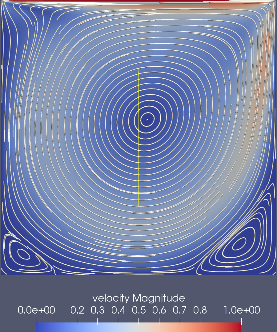
(b) D-B Test 7

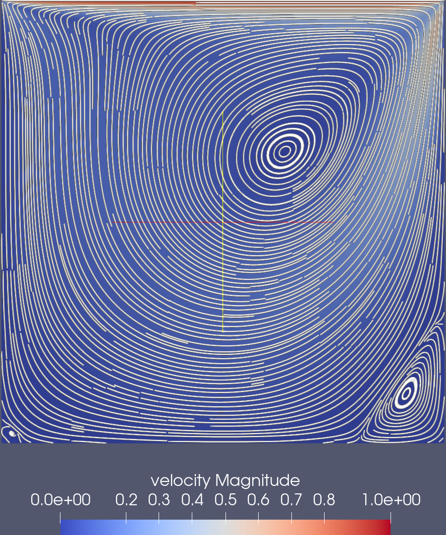
(c) D-B-F Test 7

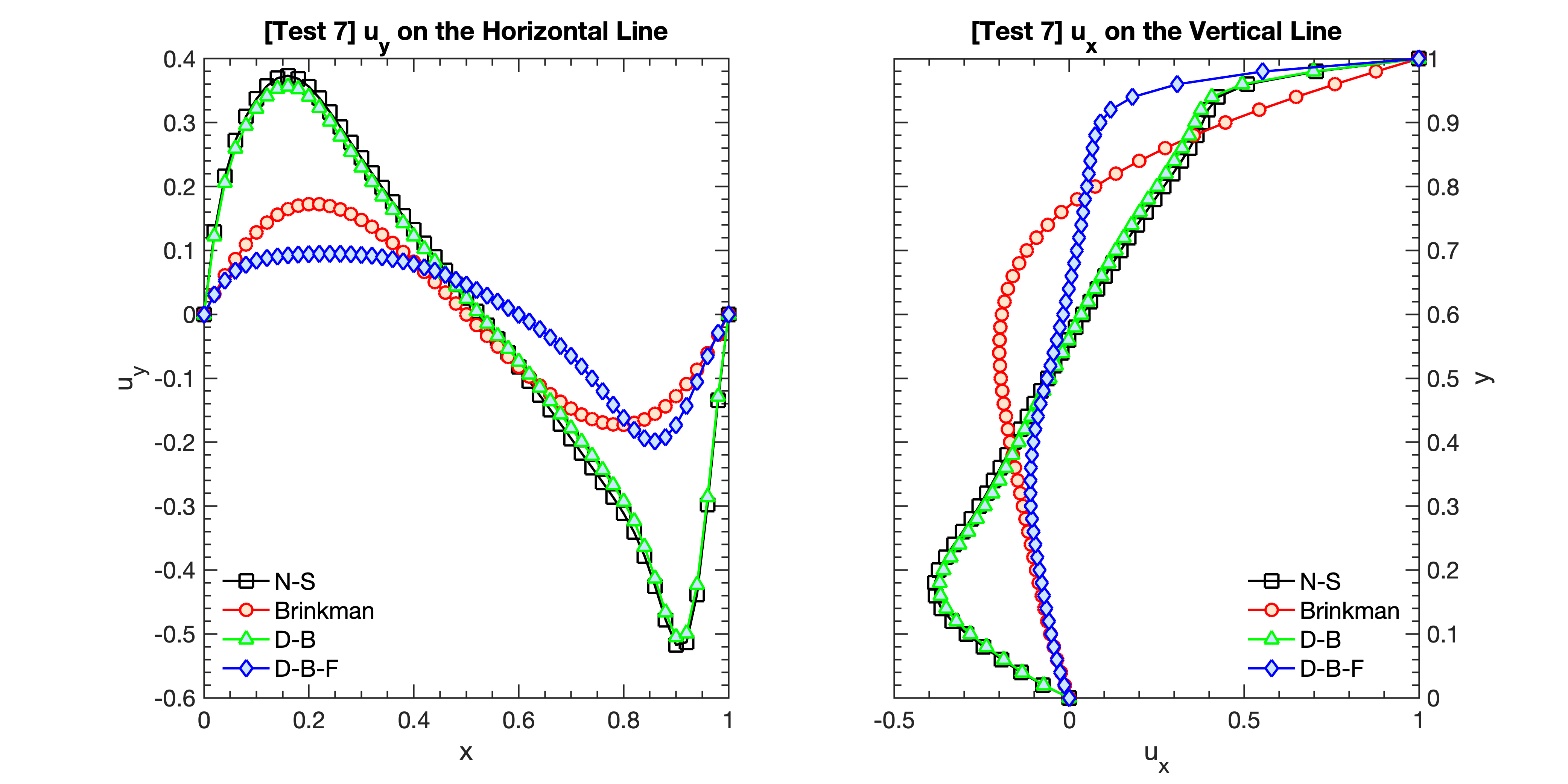
(d) Velocity on the center line

Figure 12: [GROUP II] Test 7. Velocity profiles: (a) Brinkman, (b) Darcy-Brinkman, (c) Darcy-Brinkman-Forchheimer, and (d) velocity on the reference lines using the Brinkman, Darcy-Brinkman, and Darcy-Brinkman-Forchheimer models, compared with the Navier-Stokes model. Test 7 has dimensionless numbers of 1000 for $Re$ and 2.5e-1 for $Da$.

Figure 12 illustrates the distinguishing effect of the inertial resistance. Similarly, as depicted in Figure 8, the deviation of the full nonlinear D-B-F model is even more distinctive than the previous ones. When we compare the D-B with D-B-F with the streamline results and velocities on the reference lines in Test 7 and Test 8, the D-B-F model in Test 8 with the increased $Da$ number illustrates more similar streamlines to the D-B, possessing larger area for the first eddy near the cross (see (e), (f) in Figure 11 and (b), (c) in Figure 12).

$\bullet$ Forchheimer coefficient, $c_{F}=0.4$ vs. $c_{F}=0.6$:

We further test with two different values of $c_{F}$ for the D-B-F model: $c_{F}=0.4$ and $c_{F}=0.6$. Although it is not severe, the effect of the Forchheimer term can be found, using the same $Re$ and $Da$ used in Test 7 and Test 9 in GROUP II. From (a) and (b) in Figure 13, the delay effect resulting from the inertial resistance is also confirmed; The location of the primary eddy center of (b) is higher than that of (a), occupying a smaller area. Note that all the vortices are smaller in (b) and (d) than those of (a) and (c) due to the increased value of $c_{F}=0.6$. From Figure 13, when we compare Test 7 with Test 9 with the same $c_{F}$, i.e., $c_{F}=0.4$ or $c_{F}=0.6$, we also confirm that the inertial resistance compared to $Da$ and $Re$ for Test 7 is relatively larger than that for Test 9.

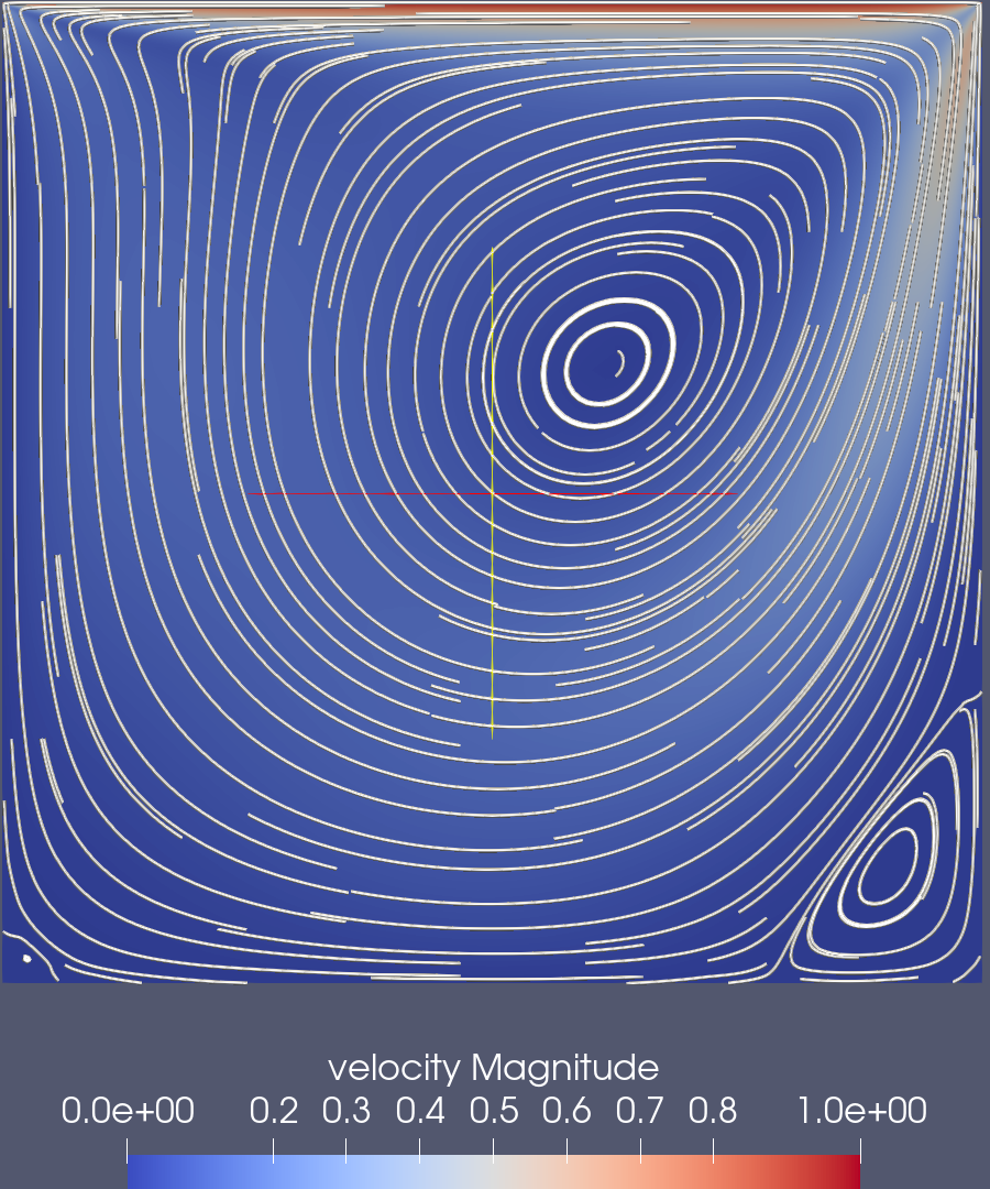
(a) D-B-F Test 7: $c_{F}=0.4$

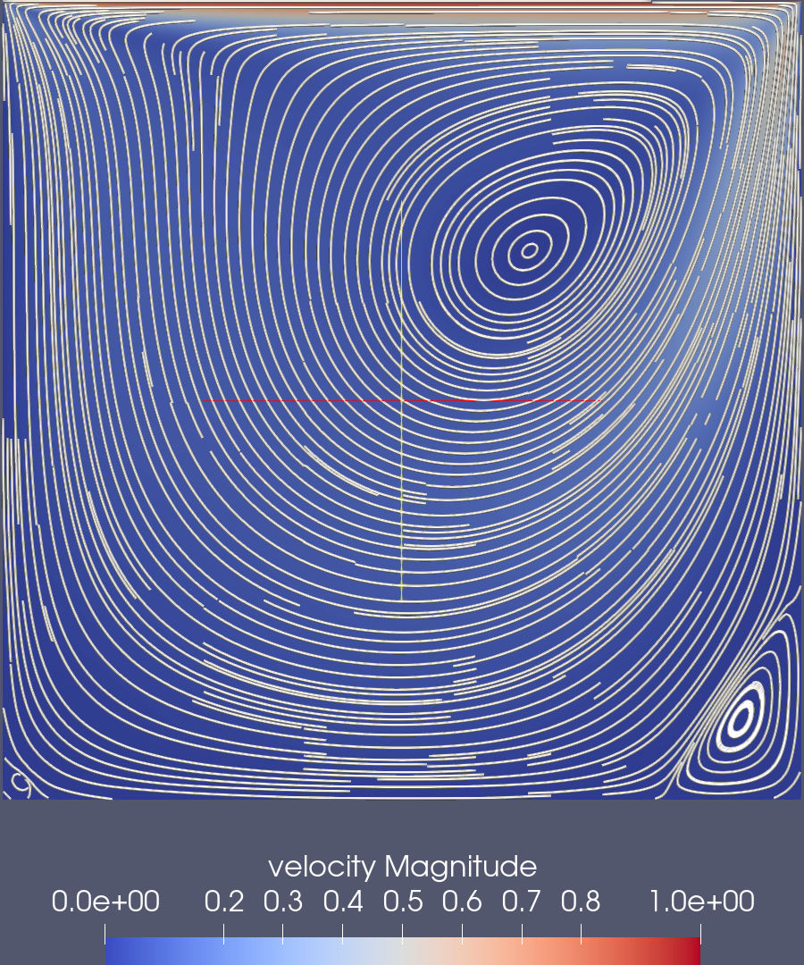
(b) D-B-F Test 7: $c_{F}=0.6$

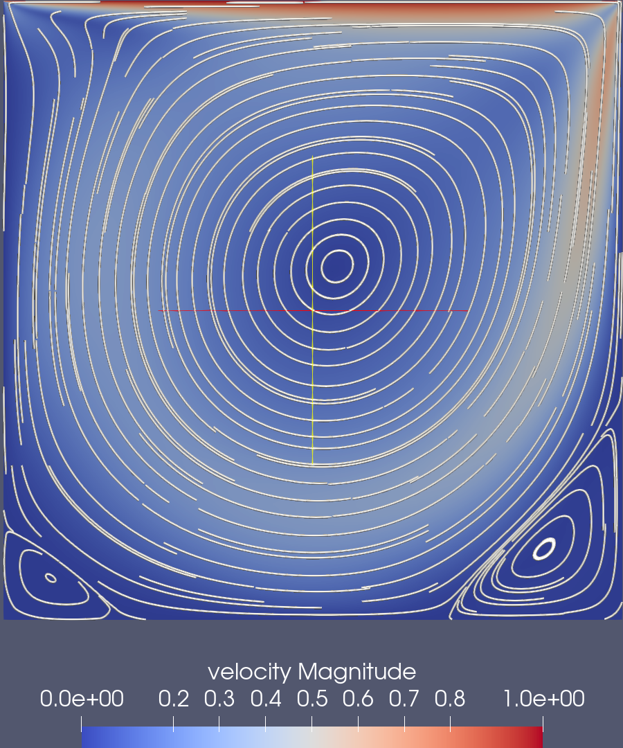
(c) D-B-F Test 9: $c_{F}=0.4$

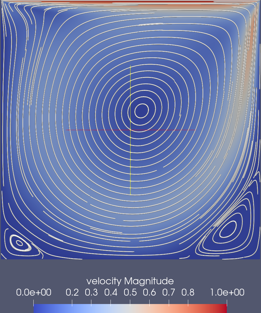
(d) D-B-F Test 9: $c_{F}=0.6$

Figure 13: [GROUP II] Test 7 and 9. Velocity streamlines $c_{F}=0.4$ (left) vs. $c_{F}=0.6$ (right). Test 7 and 9 have dimensionless numbers of 1000 for $Re$ and 2.5e-1 and 2.5e+1 for $Da$, respectively.

4.3.3 Summary on GROUP I and GROUP II results

Depending on the parameters, three models, i.e., the linearized Brinkman, Darcy-Brinkman, and Darcy-Brinkman-Forchheimer, sometimes behave similarly or depart from one another. For example, the Darcy-Brinkman is close to the Brinkman when $Re\times Da<1.0$ (GROUP I), but it is similar to the Navier-Stokes when $Re\times Da>1.0$ (GROUP II). The Brinkman can model correctly within the small $Da$ values (or $Re\times Da<1.0$), but not in the large $Da$ (or $Re\times Da>1.0$). The detailed findings for each group are what follows. For $Re\times Da<1.0$,

• Few distinctions are found in velocity profiles between the three models, i.e., the linearized Brinkman, Darcy-Brinkman, and Darcy-Brinkman-Forchheimer. Within these models, we identify the flow is controlled mainly by the viscous resistance with small $Da$ values.

• The linearized Brinkman and Darcy-Brinkman (without the inertial resistance term) models are closer to each other as little convection exists and they have the viscous resistance only.

• The linearized Brinkman can also be replaced with the Darcy-Brinkman-Forchheimer in GROUP I without much error. Little deviations that can be discerned by the Darcy-Brinkman-Forchheimer model have started, implying the intermediate regime or weak inertial regime [43].

Meanwhile, for $Re\times Da>1.0$,

• The distinctions of each model are clearly shown with its different location and size of primary, secondary, and tertiary vortices. The Forchheimer term reduces the effect and size of the vortices with the inertial resistance coefficient, which is known to depend on hydraulic properties of the porous medium.

• A rather abrupt change in flow patterns for the Darcy-Brinkman model is identified during the flow regime change, i.e., the laminar to turbulent, when $Re$ values are increased. And the Darcy-Brinkman model is the closest to the Navier-Stokes as it is homogenized from it [44].

• Since the Darcy-Brinkman-Forchheimer model has the inertial resistance, the change of flow regime is delayed under the equivalent inertial and viscous forces.

5 Conclusion

This work presents a stabilized finite element discretization of the full nonlinear steady Darcy-Brinkman-Forchheimer model of the porous medium, also highlighting the effect of dimensionless constants and the role of the Forchheimer term in the steady lid-driven cavity flow. We employ a beneficial Grad-Div stabilization technique and implement a Schur complement-based preconditioner for the established linear solver.

The efficient preconditioning strategy results in a few Newton’s iteration number even with the full nonlinear model, yielding the stable and convergent numerical solutions against the spurious oscillations that may occur from the inf-sup and discontinuous boundary conditions for the lid-driven cavity flow with relatively high Reynolds number problem for the porous media. Moreover, local mesh adaptivity works effectively for the large scale sparse problem via efficient and independent procedure. With all these approaches, different viscous and inertial resistances are applied, and we find that the full nonlinear Darcy-Brinkman-Forchheimer model can position itself in between the linearized Brinkman and Darcy-Brinkman/Navier-Stokes in the turbulent flow regime due to the role of Forchheimer term. When the $Da$ or $Re$ is significantly low, the model can replace the Brinkman, but it also can capture a very minute regime change as the $Da$ gets increased.

Meantime, the study still needs to be further investigated relating to (but not limited to) more realistic fluid properties and physics such as porosity/permeability variations and Reynolds number based on the experimental reference values (e.g., the reference distance and discharge), and multi-phase flow regime with fluid pressure and capillarity. Moreover, the relation between the dimensionless Forchheimer coefficient and real phenomena or the physical implication of coefficient is still unknown. In terms of computational performance, the study still lacks the in-depth and comprehensive knowledge on appropriate selection of the Augmented Lagrangian parameter for its full efficiency.

The proposed solver and algorithm for the Darcy-Brinkman-Forchheimer model, with its robustness in the stability and convergence of computation on incompressible turbulent flow, can be expanded and utilized straightforwardly to study other flow states or physics, such as the heat flow in the porous medium. A more challenging problem is to expand the model investigated in this study and develop a coupling model of the nonlinear flow and mechanics of porous media (e.g., the subsurface flow and geomechanics), i.e., the Forchheimer model for the non-Darcy flow and nonlinear mechanics such as the strain-limiting theories of elasticity [80, 81, 82, 83, 84, 85] and stuying flow in porous media containing network of fractures modeled by surface mechanics [86]. Devising a numerical method for these multi-physics models would also be a significant challenge.

References

- [1] K Vafai and SJin Kim. On the limitations of the brinkman-forchheimer-extended darcy equation. International Journal of Heat and Fluid Flow, 16(1):11–15, 1995.
- [2] DA Nield. Non-darcy effects in convection in a saturated porous medium. In Proc. Seminar DSIR and CSIRO Inst. Phys. Sci, pages 129–139, 1984.
- [3] D Munaf, AS Wineman, KR Rajagopal, and DW Lee. A boundary value problem in groundwater motion analysis—comparison of predictions based on darcy’s law and the continuum theory of mixtures. Mathematical Models and Methods in Applied Sciences, 3(02):231–248, 1993.
- [4] K. R. Rajagopal. On a hierarchy of approximate models for flows of incompressible fluids through porous solids. Mathematical Models and Methods in Applied Sciences, 17(02):215–252, 2007.
- [5] Shriram Srinivasan, Andrea Bonito, and Kumbakonam R Rajagopal. Flow of a fluid through a porous solid due to high pressure gradients. Journal of Porous Media, 16(3), 2013.
- [6] D.D. Joseph, D.A. Nield, and G. Papanicolaou. Nonlinear equation governing flow in a saturated porous medium. Water Resources Research, 18(4):1049–1052, 1982.
- [7] H. Brinkman. A calculation of the viscous force exerted by a flowing fluid on a dense swarm of particles. Applied Scientific Research, 1, 1949.
- [8] G. Juncu. Brinkman-Forchheimer-Darcy flow past an impermeable sphere embedded in a porous medium. Analele Stiintifice ale Universitatii Ovidius Constanta, 23(3):97–112, 2015.
- [9] Y. Jin and A.V. Kuznetsov. Turbulence modeling for flows in wall bounded porous media: An analysis based on direct numerical simulations. Physics of Fluids, 29:045102, 2017.
- [10] N. Jouybari, M. Maerefat, and M. Nimvari. A pore scale study on turbulent combustion in porous media. Heat and Mass Transfer, 52(2):269–280, 2016.
- [11] A.A. Avramenko, I.V. Shevchuk, M.M. Kovetskaya, and Y.Y. Kovetska. Darcy–brinkman–forchheimer model for film boiling in porous media. Transport in Porous Media, 134:503–536, 2020.
- [12] J. Kim, G. Luo, and C.-Y. Wang. Modeling two-phase flow in three-dimensional complex flow-fields of proton exchange membrane fuel cells. Journal of Power Sources, 365:419–429, 2017.
- [13] T. B. Gatski. Review of incompressible fluid flow computations using the vorticity-velocity formulation. Applied Numerical Mathematics, 7(3):227–239, 1991.
- [14] P. M. Gresho. Incompressible fluid dynamics: some fundamental formulation issues. Annual review of fluid mechanics, 23(1):413–453, 1991.
- [15] S. Brenner and L.R. Scott. The Mathematical Theory of Finite Element Methods. Springer, 2002.
- [16] D. Boffi, F. Brezzi, and M. Fortin. Mixed Finite Element Methods and Applications. Springer, 2013.
- [17] V. P. Vallalaa, R. Sadr, and J. N. Reddy. Higher order spectral/hp finite element models of the navier–stokes equations. International Journal of Computational Fluid Dynamics, 28(1-2):16–30, 2014.
- [18] N. Kim and J. N. Reddy. A spectral/hp least-squares finite element analysis of the carreau–yasuda fluids. International Journal for Numerical Methods in Fluids, 82(9):541–566, 2016.
- [19] M. O. Deville, P. F. Fischer, and E. H. Mund. High-order methods for incompressible fluid flow, volume 9. Cambridge university press, 2002.
- [20] P. N. Shankar. The eddy structure in stokes flow in a cavity. Journal of Fluid mechanics, 250:371–383, 1993.
- [21] R. Srinivasan. Accurate solutions for steady plane flow in the driven cavity. i. stokes flow. Zeitschrift für angewandte Mathematik und Physik ZAMP, 46(4):524–545, 1995.
- [22] C. Y. Wang. The recirculating flow due to a moving lid on a cavity containing a darcy–brinkman medium. Applied mathematical modelling, 33(4):2054–2061, 2009.
- [23] M. S. Muddamallappa, D. Bhatta, and D. N. Riahi. Numerical investigation on marginal stability and convection with and without magnetic field in a mushy layer. Transport in porous media, 79:301–317, 2009.
- [24] J. Shen. Hopf bifurcation of the unsteady regularized driven cavity flow. Journal of Computational Physics, 95(1):228–245, 1991.
- [25] E. Barragy and G. F. Carey. Stream function-vorticity driven cavity solution using p finite elements. Computers & Fluids, 26(5):453–468, 1997.
- [26] A. N. Brooks and T. J. R. Hughes. Streamline upwind/petrov-galerkin formulations for convection dominated flows with particular emphasis on the incompressible navier-stokes equations. Computer methods in applied mechanics and engineering, 32(1-3):199–259, 1982.
- [27] D-G. Wang and Q.-X. Shui. Supg finite element method based on penalty function for lid-driven cavity flow up to . Acta Mechanica Sinica, 32(1):54–63, 2016.
- [28] T. E. Tezduyar and Y. Osawa. Finite element stabilization parameters computed from element matrices and vectors. Computer Methods in Applied Mechanics and Engineering, 190(3-4):411–430, 2000.
- [29] T. E. Tezduyar and M. Senga. Stabilization and shock-capturing parameters in supg formulation of compressible flows. Computer methods in applied mechanics and engineering, 195(13-16):1621–1632, 2006.
- [30] L. P. Franca and S. L. Frey. Stabilized finite element methods: Ii. the incompressible navier-stokes equations. Computer Methods in Applied Mechanics and Engineering, 99(2-3):209–233, 1992.
- [31] P. Hansbo and A. Szepessy. A velocity-pressure streamline diffusion finite element method for the incompressible navier-stokes equations. Computer Methods in Applied Mechanics and Engineering, 84(2):175–192, 1990.
- [32] O. Botella and R. Peyret. Benchmark spectral results on the lid-driven cavity flow. Computers & Fluids, 27(4):421–433, 1998.
- [33] C. Davies and P. W. Carpenter. A novel velocity–vorticity formulation of the navier–stokes equations with applications to boundary layer disturbance evolution. Journal of computational physics, 172(1):119–165, 2001.
- [34] C. H. Whiting and K. E. Jansen. A stabilized finite element method for the incompressible navier–stokes equations using a hierarchical basis. International Journal for Numerical Methods in Fluids, 35(1):93–116, 2001.
- [35] M. Braack, E. Burman, V. John, and G. Lube. Stabilized finite element methods for the generalized oseen problem. Computer Methods in Applied Mechanics and Engineering, 196(4-6):853–866, 2007.
- [36] M. A. Olshanskii. A low order galerkin finite element method for the navier–stokes equations of steady incompressible flow: a stabilization issue and iterative methods. Computer Methods in Applied Mechanics and Engineering, 191(47-48):5515–5536, 2002.
- [37] L. Zhao and T. Heister. The deal.ii tutorial step-57: The incompressible, stationary navier stokes equations. Zenodo, 2017.
- [38] M. Olshanskii, G. Lube, T. Heister, and J. Löwe. Grad–div stabilization and subgrid pressure models for the incompressible Navier–Stokes equations. Computer Methods in Applied Mechanics and Engineering, 198(49-52):3975–3988, 2009.
- [39] D.W. Kelly, J.P. De S.R. Gago, O.C. Zienkiewicz, and I. Babuska. A posteriori error analysis and adaptive processes in the finite element method: Part i-error analysis. International journal for numerical methods in engineering, 19(11):1593–1619, 1983.
- [40] U. Ghia, K.N. Ghia, and C.T. Shin. High-re solutions for incompressible flow using the Navier-Stokes equations and a multigrid method. Journal of Computational Physics, 48:387–411, 1982.
- [41] M. Firdaouss, J.L. Guermond, and P. Le Quéré. Nonlinear corrections to Darcy’s law at low Reynolds numbers. Journal of Fluid Mechanics, 343:331–350, 1997.
- [42] F. Cimolin and M. Discacciati. Navier-Stokes/Forchheimer models for filtration through porous media. Applied Numerical Mathematics, 72:205–224, 2013.
- [43] R.W. Zimmerman, A. Al-Yaarubi, C.C. Pain, and C.A. Grattoni. Non-linear regimes of fluid flow in rock fractures. International Journal of Rock Mechanics and Mining Sciences, 41:163–169, 2004.
- [44] Z. Chen, S.L. Lyons, and G. Qin. Derivation of the forchheimer law via homogenization. Transport in Porous Media, 44:325–335, 2001.
- [45] I.F. MacDonald, M.S. El-Sayed, K. Mow, and F.A.L. Dullien. Flow through porous media: the ergun equation revisited. Indust. Chem. Fundam., 18:199–208, 1979.
- [46] S. Ergun. Fluid flow through packed columns. Chemical Engineering Progress, 48(2):89–94, 1952.
- [47] D. Yang, Z. Xue, and S.A. Mathias. Analysis of momentum transfer in a lid-driven cavity containing a brinkman–forchheimer medium. Transport in Porous Media, 92:101–118, 2012.
- [48] C. Bruneau and I. Mortazavi. Numerical modeling and passive flow control using porous media. Computers and Fluids, 37:488–498, 2008.
- [49] P. Angot. Analysis of singular perturbation on the Brinkman problem for fictitious domain models of viscous flows. Mathematical Methods in the Applied Sciences, 22:1395–1412, 1999.
- [50] K. Khadra, P. Angot, S. Parneix, and J. Caltagirone. Fictitious domain approach for numerical modeling of Navier-Stokes equations. International Journal for Numerical Methods in Fluids, 34:651–684, 2000.
- [51] R. Gutt and T. Groşan. On the lid-driven problem in a porous cavity. a theoretical and numerical approach. Applied Mathematics and Computation, 266:1070–1082, 2015.
- [52] Sergey Charnyi, Timo Heister, Maxim A Olshanskii, and Leo G Rebholz. Efficient discretizations for the emac formulation of the incompressible Navier–Stokes equations. Applied Numerical Mathematics, 141:220–233, 2019.
- [53] Carl T Kelley. Solving nonlinear equations with Newton’s method. SIAM, 2003.
- [54] James M Ortega and Werner C Rheinboldt. Iterative solution of nonlinear equations in several variables. SIAM, 2000.
- [55] Philippe G Ciarlet. The finite element method for elliptic problems. SIAM, 2002.
- [56] H. C. Yoon and J. Kim. Spatial stability for the monolithic and sequential methods with various space discretizations in poroelasticity. International Journal for Numerical Methods in Engineering, 114(7):684–718, 2018.
- [57] Alexandre Ern and Jean-Luc Guermond. Theory and practice of finite elements, volume 159. Springer Science & Business Media, 2013.
- [58] Vivette Girault and Pierre-Arnaud Raviart. Finite Element Methods for Navier-Stokes Equations: Theory and Algorithms, volume 5. Springer Science & Business Media, 2012.
- [59] Timo Heister and Gerd Rapin. Efficient augmented lagrangian-type preconditioning for the oseen problem using grad-div stabilization. International Journal for Numerical Methods in Fluids, 71(1):118–134, 2013.
- [60] Naveed Ahmed. On the grad-div stabilization for the steady oseen and Navier-Stokes equations. Calcolo, 54(1):471–501, 2017.
- [61] Liang Zhao. A numerical method for the Navier Stokes Equations in a Velocity-Vorticity Form. PhD thesis, Clemson University, 2018.
- [62] M. Benzi and M.A. Olshanskii. An augmented lagrangian-based approach to the oseen problem. SIAM Journal on Scientific Computing, 28(6):2095–2113, 2006.
- [63] E. W. Jenkins, V. John, A. Linke, and L. G. Rebholz. On the parameter choice in grad-div stabilization for the stokes equations. Advances in Computational Mathematics, 40(2):491–516, 2014.
- [64] G. Matthies, N. I. Ionkin, G. Lube, and L. Röhe. Some remarks on residual-based stabilisation of inf-sup stable discretisations of the generalised oseen problem. Computational methods in applied mathematics, 9:368–390, 2009.
- [65] Yousef Saad. Iterative methods for sparse linear systems. SIAM, 2003.
- [66] Timothy A Davis. Direct methods for sparse linear systems. SIAM, 2006.
- [67] Timothy A Davis. Algorithm 832: Umfpack v4. 3—an unsymmetric-pattern multifrontal method. ACM Transactions on Mathematical Software (TOMS), 30(2):196–199, 2004.
- [68] D. Arndt, W. Bangerth, T. C. Clevenger, D. Davydov, M. Fehling, D. Garcia-Sanchez, G. Harper, T. Heister, L. Heltai, M. Kronbichler, R. M. Kynch, M. Maier, J.-P. Pelteret, B. Turcksin, and D. Wells. The deal.II library, version 9.2. Journal of Numerical Mathematics, 2020.
- [69] Youcef Saad. A flexible inner-outer preconditioned gmres algorithm. SIAM Journal on Scientific Computing, 14(2):461–469, 1993.
- [70] Philip M Gresho and Robert L Lee. Don’t suppress the wiggles—they’re telling you something! Computers & Fluids, 9(2):223–253, 1981.
- [71] Rüdiger Verfürth. A posteriori error estimation and adaptive mesh-refinement techniques. Journal of Computational and Applied Mathematics, 50(1-3):67–83, 1994.
- [72] JP De S.R. Gago, DW Kelly, OC Zienkiewicz, and I Babuska. A posteriori error analysis and adaptive processes in the finite element method: Part ii—adaptive mesh refinement. International journal for numerical methods in engineering, 19(11):1621–1656, 1983.
- [73] OC Zienkiewicz and JZ Zhu. Adaptivity and mesh generation. International Journal for Numerical Methods in Engineering, 32(4):783–810, 1991.
- [74] AS Usmani. Solution of steady and transient advection problems using an h-adaptive finite element method. International Journal of Computational Fluid Dynamics, 11(3-4):249–259, 1999.
- [75] Gustavo A Ríos Rodriguez, Mario A Storti, Ezequiel J López, and Sofía S Sarraf. An h-adaptive solution of the spherical blast wave problem. International Journal of Computational Fluid Dynamics, 25(1):31–39, 2011.
- [76] Michael Holst and Sara Pollock. Convergence of goal-oriented adaptive finite element methods for nonsymmetric problems. Numerical Methods for Partial Differential Equations, 32(2):479–509, 2016.
- [77] Wolfgang Bangerth and Rolf Rannacher. Adaptive finite element methods for differential equations. Birkhäuser, 2013.
- [78] Mark Ainsworth and J Tinsley Oden. A posteriori error estimation in finite element analysis, volume 37. John Wiley & Sons, 2011.
- [79] J. Bears. Dynamics of fluids in porous media. New York: American Elsevier Pub. Co., Inc, 1972.
- [80] S. Lee, H. C. Yoon, and S. M. Mallikarjunaiah. Nonlinear strain-limiting elasticity for fracture propagation with phase-field approach. Journal of Computational and Applied Mathematics, 399:113715, 2022.
- [81] Hyun C Yoon, Sanghyun Lee, and SM Mallikarjunaiah. Quasi-static anti-plane shear crack propagation in nonlinear strain-limiting elastic solids using phase-field approach. International Journal of Fracture, 227(2):153–172, 2021.
- [82] H. C. Yoon and S. M. Mallikarjunaiah. A finite-element discretization of some boundary value problems for nonlinear strain-limiting elastic bodies. Mathematics and Mechanics of Solids, 27(2):281–307, 2022.
- [83] H. C. Yoon, S. M. Mallikarjunaiah, and D. Bhatta. Preferential stiffness and the crack-tip fields of an elastic porous solid based on the density-dependent moduli model. arXiv preprint arXiv:2212.08181, 2022.
- [84] H. C. Yoon, K. K. Vasudeva, and S. M. Mallikarjunaiah. Finite element model for a coupled thermo-mechanical system in nonlinear strain-limiting thermoelastic body. Communications in Nonlinear Science and Numerical Simulation, 108:106262, 2022.
- [85] Hyun C Yoon, SM Mallikarjunaiah, and Dambaru Bhatta. Finite element solution of crack-tip fields for an elastic porous solid with density-dependent material moduli and preferential stiffness. Advances in Mechanical Engineering, 16(2):16878132241231792, 2024.
- [86] L. A. Ferguson, M. Muddamallappa, and J. R. Walton. Numerical simulation of mode-iii fracture incorporating interfacial mechanics. International Journal of Fracture, 192:47–56, 2015.