LargeAD: Large-Scale Cross-Sensor Data Pretraining for Autonomous Driving

Abstract

Recent advancements in vision foundation models (VFMs) have revolutionized visual perception in 2D, yet their potential for 3D scene understanding, particularly in autonomous driving applications, remains underexplored. In this paper, we introduce LargeAD, a versatile and scalable framework designed for large-scale 3D pretraining across diverse real-world driving datasets. Our framework leverages VFMs to extract semantically rich superpixels from 2D images, which are aligned with LiDAR point clouds to generate high-quality contrastive samples. This alignment facilitates cross-modal representation learning, enhancing the semantic consistency between 2D and 3D data. We introduce several key innovations: i) VFM-driven superpixel generation for detailed semantic representation, ii) a VFM-assisted contrastive learning strategy to align multimodal features, iii) superpoint temporal consistency to maintain stable representations across time, and iv) multi-source data pretraining to generalize across various LiDAR configurations. Our approach delivers significant performance improvements over state-of-the-art methods in both linear probing and fine-tuning tasks for both LiDAR-based segmentation and object detection. Extensive experiments on eleven large-scale multi-modal datasets highlight our superior performance, demonstrating the adaptability, efficiency, and robustness in real-world autonomous driving scenarios. The project page can be accessible at: https://ldkong.com/LargeAD.

1 Introduction

The emergence of large language models (LLMs) [1, 2, 3, 4, 5] has transformed natural language processing, paving the way for similar breakthroughs in computer vision through vision foundation models (VFMs) such as SAM [6], X-Decoder [7], and SEEM [8]. These models have demonstrated remarkable capabilities in extracting rich pixel-level semantics from 2D images. However, extending these advancements to the 3D domain remains a largely unexplored frontier. As autonomous driving applications increasingly rely on 3D data from LiDAR sensors, there is a growing need to transfer the success of VFMs in 2D vision to 3D scene understanding [9, 10].

Accurate segmentation and detection of LiDAR point clouds are essential for safe autonomous driving and advanced driver-assistance systems [11, 12, 13, 14, 15]. Traditional LiDAR point cloud models often depend on large annotated datasets, which are costly and time-consuming to create [16, 17]. To alleviate this challenge, research has explored semi-supervised [18, 19] and weakly-supervised [17, 20] methods. However, these approaches suffer from limited generalizability, especially when faced with diverse sensor configurations, e.g., different LiDAR beam numbers, camera placements, sampling rates, and potential sensor corruptions [21, 22, 11, 23, 24, 25]. This limitation poses a significant challenge for real-world scalability.

In response, we propose LargeAD, a novel and scalable framework for 3D scene understanding that leverages large-scale data pretraining across diverse sensors. Our approach builds on recent advances in cross-modal representation learning [6, 7, 26], incorporating VFMs into the 3D domain to address several critical objectives: i) utilizing raw point clouds as input to eliminate the need for costly labels, ii) exploiting spatial and temporal cues from driving scenes for robust representation learning, and iii) ensuring generalizability to downstream datasets beyond the pretraining data. By distilling the semantic knowledge encoded in VFMs, our methodology facilitates self-supervised learning on complex 3D point clouds, particularly for autonomous driving.

A core innovation in our framework is the use of VFMs to generate semantically enriched superpixels from camera images, which are then aligned with LiDAR data to construct high-quality contrastive samples (see Fig. 1). These semantic superpixels provide enhanced 2D-3D correspondences that capture object-level coherence, reducing the errors commonly associated with over-segmentation and “self-conflict” in contrastive learning [9]. This alignment significantly improves performance in downstream tasks, including 3D object detection and segmentation.

Furthermore, the proposed framework introduces several additional innovations. First, a VFM-assisted contrastive learning strategy aligns superpixels and superpoints within a unified embedding space, addressing the cross-modal discrepancies between image and LiDAR features. Second, a superpoint temporal consistency mechanism enhances the robustness of point cloud representations across time, mitigating errors from imperfect synchronization between LiDAR and camera sensors. Finally, our multi-source data pretraining strategy leverages diverse LiDAR datasets to build a generalized model capable of adapting to different sensor configurations, further boosting the scalability.

As shown in Fig. 2, compared to state-of-the-art methods such as SLidR [27] and ST-SLidR [28], our framework introduces significant advancements: i) the use of semantically rich superpixels to resolve the “self-conflict” issue in contrastive learning, ii) the creation of high-quality contrastive samples, which lead to faster and more stable convergence, and iii) reduced computational overhead due to the more efficient superpixel generation process.

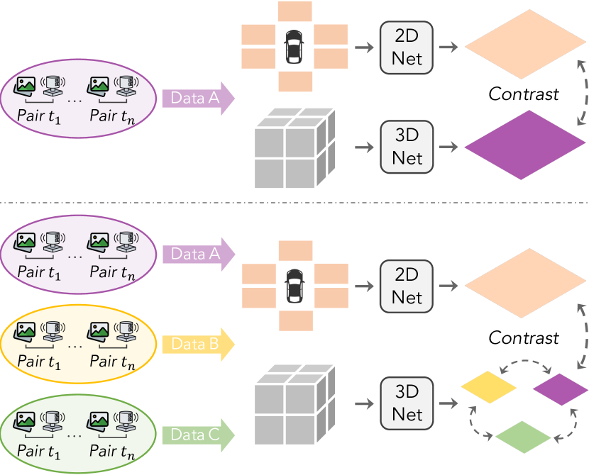
Figure 1: Comparisons between i) the conventional image-to-LiDAR data pretraining frameworks [27, 28, 9] and ii) our proposed large-scale cross-sensor data pretraining (LargeAD). Our approach combines heterogeneous data sources for representation learning, which achieves superior robustness and scalability. Different from previous work, our framework encourages representation learning across different datasets, which largely enhances the generalizability.

In summary, this paper offers the following contributions:

• We introduce LargeAD, a scalable, consistent, and generalizable framework designed for large-scale pretraining on data captured from onboard vehicle sensors, addressing the challenges of diverse LiDAR configurations and improving representation learning capabilities.

• To the best of our knowledge, this is the first comprehensive study to explore pretraining across multiple large-scale driving datasets, leveraging cross-dataset knowledge to enhance the model’s generalizability to different sensor setups and driving environments.

• Our framework incorporates several key innovations: i) VFM-based superpixel generation that enriches semantic representation, ii) VFM-assisted contrastive learning to align 2D-3D features, iii) superpoint temporal consistency to stabilize point cloud representations across time, and iv) multi-source data pretraining that ensures robustness across domains.

• Our approach demonstrates significant performance advantages over state-of-the-art methods, achieving superior results in both linear probing and fine-tuning tasks across $11$ diverse point cloud datasets, showcasing its adaptability and efficiency in real-world applications.

The remainder of this paper is organized as follows. Sec. 2 reviews the relevant literature on autonomous driving data perception and pretraining, as well as multi-dataset utilization. Sec. 3 elaborates on preliminaries of image-to-LiDAR contrastive learning. Sec. 4 presents the technical methodology behind the proposed large-scale cross-sensor pretraining framework. Finally, Sec. 5 presents the experimental validation of our approach, and Sec. 6 concludes the paper with discussions on future directions.

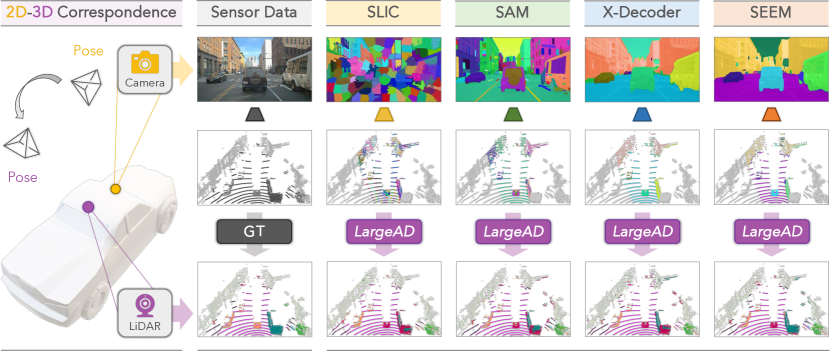
Figure 2: Illustration of image-to-LiDAR data pretraining using i) the heuristic SLIC algorithm [29] and ii) different vision foundation models (VFMs). Images in the first row are the superpixels generated by different methods, where each color represents one distinct segment. The LiDAR point clouds from the second row are the superpoints grouped by projecting superpixels to 3D using camera-LiDAR correspondence. The third row shows the linear probing results after data pretraining.

2 Related Work

In this section, we provide a thorough literature review of relevant works in the areas of LiDAR-based autonomous driving scene understanding (Sec. 2.1), popular vision foundation models (Sec. 2.2), different 3D representation learning techniques (Sec. 2.3), and multi-dataset learning and utilization in the domain of 3D object detection and LiDAR semantic segmentation (Sec. 2.4).

2.1 LiDAR-Based Scene Understanding

For autonomous vehicles, accurate and dense 3D perception is crucial for safe navigation [12, 30]. Researchers have developed various methods for point cloud segmentation, including those based on raw points [31, 32, 33, 34, 35], range views [36, 37, 38, 39, 40, 41, 42], bird’s eye views [43, 44], voxels [45, 46, 47, 48, 49], and multi-view fusion [50, 51, 52, 53, 54, 55]. Despite achieving significant advancements, these models typically rely on extensively annotated datasets, posing scalability issues [21]. To alleviate the annotation burden, recent studies have explored semi-supervised [18, 19, 56], weakly-supervised [17, 57, 58, 59, 20], and active learning [60, 61, 62] methods, as well as domain adaptation techniques [63, 64, 65, 66, 67, 68]. This work utilizes a self-supervised learning strategy, distilling knowledge from VFMs through camera-to-LiDAR associations, thereby eliminating the need for manual annotations during pretraining.

2.2 Vision Foundation Models

The field of computer vision has been transformed by the development of vision foundation models (VFMs) that leverage vast amounts of training data [69, 6] and sophisticated self-supervised learning techniques [70, 71]. Among these, the Segment Anything Model, or SAM [6], has set a new benchmark in general-purpose image segmentation, showcasing impressive zero-shot transfer capabilities across a range of downstream tasks. Other notable VFMs, such as X-Decoder [7], OpenSeeD [26], SegGPT [72], and SEEM [8], have further demonstrated the versatility of these models in handling diverse image-related tasks. This work extends the utilization of VFMs to the domain of point cloud learning, capitalizing on their semantic understanding to enhance spatial and temporal cues in 3D representation learning.

2.3 Representation Learning in 3D

3D self-supervised learning has its roots in image-based techniques and typically focuses on object-centric point clouds [73, 74, 75, 76, 77] or indoor scenes [78, 79, 80, 81, 82] using pretext tasks [83, 84, 85, 86, 87], contrastive learning [88, 89, 90, 91, 92, 93, 94], or mask modeling [95, 96, 97, 98]. These methods often lack the necessary scale and diversity for outdoor driving scenes [99, 100, 101]. Efforts such as PointContrast [102], DepthContrast [103], and SegContrast [104] have pioneered contrastive objectives for small-scale point clouds. Recently, Sautier et al. [27] introduced SLidR, the first method for image-to-LiDAR representation distillation in cross-modal self-supervised learning on large-scale point clouds. Mahmoud et al. [28] further refined this approach with semantically tolerant contrastive constraints and a class-balancing loss. SuperFlow [105] introduced a spatiotemporal consistency framework to efficiently capture dynamic cues across multiple timesteps. Our framework builds upon SLidR [27] by leveraging VFMs [6, 7, 8] to create a more effective cross-modal contrastive objective. We also introduce a superpoint temporal consistency regularization to enhance feature learning and robustness in diverse and dynamic real-world driving scenarios.

2.4 Multi-Dataset Utilization

Leveraging multiple datasets has emerged as a promising approach for improving the generalization of LiDAR-based models in autonomous driving [106]. Recent works like MDT3D [107] and MS3D++ [108] explored multi-source training for 3D object detection, while addressing challenges such as label space conflicts. Similarly, methods like COLA [109] and M3Net [110] utilized unified label spaces for semantic segmentation, demonstrating the advantages of multi-dataset learning. In this work, we extend these efforts by proposing a multi-source pretraining strategy that incorporates data from diverse LiDAR datasets, each with unique sensor setups and conditions [111, 112, 113]. By aligning 2D and 3D features across different sources, our approach improves cross-modal consistency and robustness. To the best of our knowledge, this is the first comprehensive study on multi-source pretraining for image-to-LiDAR representation learning, allowing our framework to generalize more effectively across varied driving environments and sensor configurations.

3 Image-to-LiDAR Data Pretraining

In this section, we elaborate on the technical details of the image-to-LiDAR pretraining. We first present the preliminaries (Sec. 3.1), followed by the introduction of superpixel-driven contrastive learning (Sec. 3.2), and conclude with the description of the contrastive learning objective (Sec. 3.3).

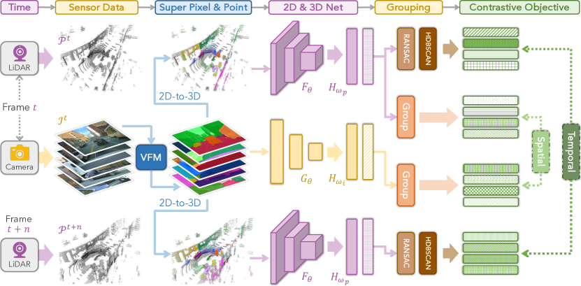
Figure 3: Overview of the VFM-driven image-to-LiDAR contrastive learning framework. Given a pair of LiDAR point cloud $\mathcal{P}^{t}$ and camera image $\mathcal{I}^{t}$ captured at timestamp $t$, along with another LiDAR point cloud $\mathcal{P}^{t+n}$ captured at timestamp $t+n$, we generate semantic superpixels using vision foundation models (VFMs). The corresponding superpoints are obtained by projecting image pixels onto the point cloud. Two key objectives are established: i) spatial contrastive learning between paired LiDAR and camera features, and ii) temporal consistency regularization between point segments from $\mathcal{P}^{t}$ and $\mathcal{P}^{t+n}$.

3.1 Problem Formulation

Let us define a point cloud $\mathcal{P}=\{\mathbf{p}_{i},\mathbf{e}_{i}\mid i=1,\ldots,N\}$ consisting of $N$ points collected by a LiDAR sensor. Each point $\mathbf{p}_{i}\in\mathbb{R}^{3}$ denotes the 3D coordinates, while $\mathbf{e}_{i}\in\mathbb{R}^{L}$ represents its feature embedding, such as intensity, elongation, etc. This work aims to transfer knowledge from a set of surround-view images $\mathcal{I}=\{\mathbf{I}_{i}\mid i=1,\ldots,V\}$, captured by a total of $V$ synchronized RGB cameras, to the point cloud $\mathcal{P}$. Each image $\mathbf{I}\in\mathbb{R}^{3\times H\times W}$ has a spatial resolution defined by height $H$ and width $W$.

Given that the LiDAR and camera sensors are assumed to be well-calibrated, each LiDAR point $\mathbf{p}_{i}=(x_{i},y_{i},z_{i})$ can be projected onto the image plane as a pixel $\hat{\mathbf{p}}_{i}=(u_{i},v_{i})$ using the following coordinate transformation:

$$[u_{i},v_{i},1]^{\text{T}}=\frac{1}{z_{i}}\times\Gamma_{K}\times\Gamma_{c\leftarrow l}\times[x_{i},y_{i},z_{i}]^{\text{T}}~,$$ (1)

where $\Gamma_{K}$ denotes the camera intrinsic matrix, and $\Gamma_{c\leftarrow l}$ is the transformation matrix from the LiDAR to the camera coordinate system.

Previous studies[27, 28] employ the unsupervised SLIC algorithm [29] to aggregate image regions with similar RGB attributes into a set of superpixels, denoted as $\Phi_{\mathcal{S}}=\{\mathbf{s}_{m}\mid m=1,\ldots,M\}$. Subsequently, the corresponding superpoint set $\Phi_{\mathcal{O}}=\{\mathbf{o}_{m}\mid m=1,\ldots,M\}$ is derived using Eq. 1. To facilitate the knowledge transfer from images to the LiDAR domain, these methods [27, 28] usually conduct cross-modal contrastive learning between the representations of superpixels and superpoints.

3.2 Superpixel-Driven Contrastive Learning

Earlier methods like PPKT [114] align image pixels with corresponding LiDAR points through contrastive learning. However, PPKT [114] tends to struggle with several limitations when applied to sparse point cloud data, such as misalignment due to viewpoint differences, inadequate local semantic modeling, imbalanced weighting of dense and sparse regions, and poor handling of false negatives. While it performs well in dense regions (e.g., near vehicles), its effectiveness drops significantly in sparse areas, limiting its overall generalization.

To overcome these issues, SLidR [27] introduces a superpixel-driven distillation approach using the SLIC algorithm [29] to group similar pixels into coherent superpixels. By employing contrastive learning between superpixels in images and superpoints in LiDAR data, SLidR reduces alignment errors from sensor viewpoints and enhances local semantic consistency. Aggregating features at the superpixel and superpoint levels resolves the weighting imbalance present in PPKT [114], ensuring better treatment of both dense and sparse regions. Moreover, contrastive learning over larger regions helps reduce false negatives, leading to more robust image-to-LiDAR knowledge transfer.

3.3 Contrastive Learning Objective

Let $F_{\theta_{p}}:\mathbb{R}^{N\times(3+L)}\to\mathbb{R}^{N\times C}$ represent a LiDAR point cloud encoder with trainable parameters $\theta_{p}$, which processes a point cloud $\mathcal{P}$ and outputs a $C$–dimensional feature for each point. Additionally, let $G_{\theta_{i}}:\mathbb{R}^{H\times W\times 3}\to\mathbb{R}^{\frac{H}{s}\times\frac{W}{s}\times E}$ be an image encoder with parameters $\theta_{i}$, initialized from 2D self-supervised pretrained models. To compute the superpixel-driven contrastive loss, we construct trainable projection heads $H_{\omega_{p}}$ and $H_{\omega_{i}}$ which map the 3D point features and 2D image features into the same $D$-dimensional embedding space. The point projection head $H_{\omega_{p}}:\mathbb{R}^{N\times C}\to\mathbb{R}^{N\times D}$ is a linear layer followed by $\ell_{2}$-normalization. The image projection head $H_{\omega_{i}}:\mathbb{R}^{\frac{H}{s}\times\frac{W}{s}\times E}\to\mathbb{R}^{H\times W\times D}$ consists of a convolution layer with a $1\times 1$ kernel, followed by a fixed bi-linear interpolation layer in the spatial dimension, and outputs with $\ell_{2}$-normalization.

The goal is to distill the 2D network’s knowledge into the 3D network, ensuring that each semantic superpoint feature closely correlates with its corresponding semantic superpixel feature. Specifically, the superpixels $\Phi_{\mathcal{S}}$ and superpoints $\Phi_{\mathcal{O}}$ are used to group pixel and point embedding features, respectively. An average pooling operation is applied to the grouped pixel and point embeddings to obtain superpixel embedding features $\mathbf{Q}\in\mathbb{R}^{M\times D}$ and superpoint embedding features $\mathbf{K}\in\mathbb{R}^{M\times D}$. The contrastive loss $\mathcal{L}^{\text{slic}}=\mathcal{L}\left(\mathbf{Q},\mathbf{K}\right)$ is then defined as follows:

$$-\frac{1}{M}{\sum_{i=1}^{M}\log\left[\frac{e^{\left(\left<\mathbf{q}_{i},\mathbf{k}_{i}\right>/\tau\right)}}{\sum_{j\neq i}e^{\left(\left<\mathbf{q}_{i},\mathbf{k}_{j}\right>/\tau\right)}+e^{\left(\left<\mathbf{q}_{i},\mathbf{k}_{i}\right>/\tau\right)}}\right]},$$ (2)

where $\left<\mathbf{q}_{i},\mathbf{k}_{j}\right>$ represents the scalar product between superpoint and superpixel embedding features, measuring their similarity. $\tau$ is a temperature parameter used to scale the similarity scores.

4 LargeAD: A Scalable, Versatile, and Generalizable Framework

In this section, we present the technical details of the proposed framework. We begin by introducing our VFM-based superpixel generation approach (Sec. 4.1), followed by the explanation of semantic spatial consistency learning (Sec. 4.2). Next, we discuss the instance superpoint temporal consistency (Sec. 4.3), and conclude with the description of multi-source data pretraining (Sec. 4.4), culminating with a summary of the overall framework (Sec. 4.5).

4.1 Superpixel Generation from Foundation Models

Previous works have utilized SLIC [29] to group visually similar image regions into superpixels. However, SLIC often over-segments semantically coherent areas (see Fig.2), which poses challenges for contrastive learning, particularly due to the “self-conflict” phenomenon. This occurs when semantically similar superpixels are incorrectly treated as negative samples[115]. While [28] introduced a semantically tolerant loss to address this issue, the lack of high-level semantic understanding in SLIC exacerbates the difficulties in contrastive learning. To overcome these challenges, we generate semantic superpixels using vision foundation models (VFMs), which provide semantically rich superpixels and significantly improve the representation learning for both near and far points in the LiDAR point cloud (see Fig. 5).

Instead of relying on low-level RGB features, our approach enhances superpixel generation by leveraging VFMs derived from large-scale pretrained image encoders [6, 8, 26, 7]. Unlike SLIC, VFMs capture high-level semantic information (as shown in Fig. 2), allowing us to create more semantically meaningful superpixel sets, denoted as $\widehat{\Phi}_{\mathcal{S}}=\left\{\left\{\mathbf{s}_{m_{v}}\mid m_{v}=1,\ldots,M_{v}\right\}\mid M_{v}\ll M\right\}$. The generation process begins with the creation of semantic masks via prompts. By incorporating more abstract features, VFMs effectively address the “self-conflict” issue by grouping semantically similar regions more coherently, reducing the risk of misclassification during contrastive learning. As a result, the generated superpixels more accurately represent object semantics rather than just visual similarities. The corresponding superpoint set, $\widehat{\Phi}_{\mathcal{O}}=\left\{\left\{\mathbf{o}_{m_{v}}\mid m_{v}=1,\ldots,M_{v}\right\}\mid M_{v}\ll M\right\}$, is established using Eq. 1, ensuring proper alignment between the 2D image features and the 3D LiDAR point features.

Our VFM-assisted superpixels serve two primary purposes: first, they enhance the semantic richness of the generated superpixels, and second, they improve the alignment between 2D image features and the 3D LiDAR point cloud. By leveraging the high-level semantic features provided by VFMs, our approach effectively addresses issues like misalignment and feature inconsistency that often arise in traditional methods based on low-level RGB features. This enhanced semantic coherence between superpixels and superpoints reduces the occurrence of false negatives in contrastive learning. As a result, the improved feature alignment ensures that both superpixels and their corresponding superpoints more accurately reflect the underlying object semantics, ultimately leading to better performance in tasks such as 3D object detection and segmentation.

4.2 Semantic Spatial Consistency Learning

Building upon the semantic superpixels generated by VFMs, as discussed in Sec. 4.1, we introduce a VFM-assisted contrastive learning framework that leverages these high-level visual features. The primary goal is to align superpixels with superpoints in a unified semantic space, ensuring that corresponding regions across different modalities are treated as positive pairs during training. By incorporating VFMs, this framework improves semantic consistency between images and LiDAR point clouds, addressing the alignment challenges often encountered in earlier methods. This approach enhances feature correspondence while reducing issues related to viewpoint variation and cross-modal discrepancies.

To implement this framework, we use the same trainable LiDAR point cloud encoder $F_{\theta_{p}}$ and frozen image encoder $G_{\theta_{i}}$ as described earlier, extracting features from the LiDAR point cloud and 2D images, respectively. For the contrastive loss, we employ the projection heads $H_{\omega_{p}}$ and $H_{\omega_{i}}$ from Sec. 3.2, projecting both point and image features into a shared $D$–dimensional embedding space. Unlike the low-level cues generated by SLIC, the superpixels produced by VFMs are enriched with semantic information, leading to more coherent and meaningful representations.

To compute the VFM-assisted contrastive loss, we apply average pooling to the pixel and point embeddings grouped by the superpixel set $\widehat{\Phi}_{\mathcal{S}}$ and the corresponding superpoint set $\widehat{\Phi}_{\mathcal{O}}$. This process yields superpixel embeddings $\widehat{\mathbf{Q}}\in\mathbb{R}^{M_{v}\times D}$ and superpoint embeddings $\widehat{\mathbf{K}}\in\mathbb{R}^{M_{v}\times D}$. The VFM-assisted contrastive loss $\mathcal{L}^{\text{vfm}}=\mathcal{L}\left(\widehat{\mathbf{Q}},\widehat{\mathbf{K}}\right)$ is formulated as follows:

$$-\frac{1}{M_{v}}{\sum_{i=1}^{M_{v}}\log\left[\frac{e^{\left(\left<\hat{\mathbf{q}}_{i},\hat{\mathbf{k}}_{i}\right>/\tau\right)}}{\sum_{j\neq i}e^{\left(\left<\hat{\mathbf{q}}_{i},\hat{\mathbf{k}}_{j}\right>/\tau\right)}+e^{\left(\left<\hat{\mathbf{q}}_{i},\hat{\mathbf{k}}_{i}\right>/\tau\right)}}\right]}.$$ (3)

The contrastive learning framework benefits from the rich semantic information provided by VFMs in several ways. First, these semantically enhanced superpixels help mitigate the “self-conflict” problem prevalent in existing approaches. Second, the high-quality contrastive samples generated by VFMs form a more coherent optimization landscape, leading to faster convergence compared to unsupervised superpixel generation methods. Finally, the use of superpixels from VFMs reduces the embedding length from hundreds (SLIC) to dozens, improving computational efficiency and accelerating the overall training process.

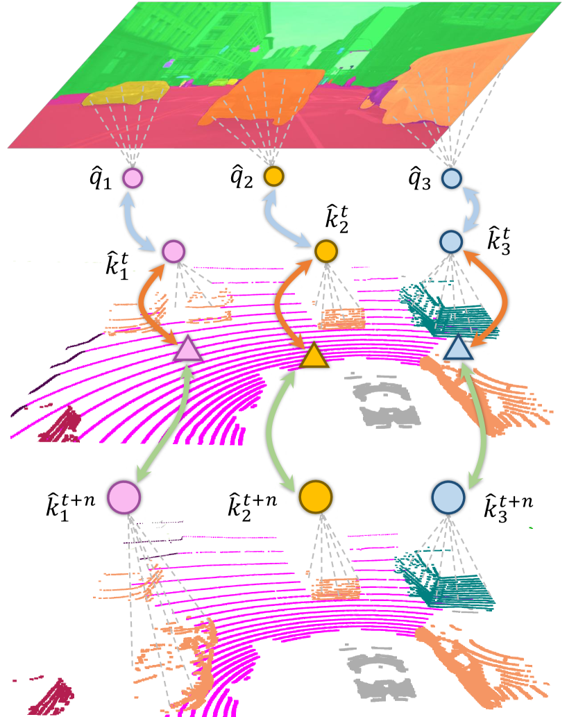
Figure 4: The positive feature correspondences of the contrastive objective in our proposed VFM-driven contrastive learning framework. The circles and triangles represent the instance-level and the point-level features, respectively.

4.3 Instance Superpoint Temporal Consistency

In real-world deployments, perfectly synchronized LiDAR and camera data are often impractical, limiting scalability. To address this, we rely on accurate geometric information from point clouds to mitigate synchronization constraints.

Implicit Geometric Clustering. We first remove the ground plane points and select the non-ground points $\mathcal{G}^{t}$ from the LiDAR point cloud $\mathcal{P}^{t}$ at timestamp $t$ using the RANSAC algorithm [116]. We then group $\mathcal{G}^{t}$ into $M_{k}$ segments, $\mathcal{K}^{t}=\{\mathcal{K}_{1}^{t},...,\mathcal{K}_{M_{k}}^{t}\}$, with the help of the HDBSCAN algorithm [117]. To map the segment views across different timestamps, we transform the LiDAR frames into a global coordinate frame, and then aggregate them. This gives the aggregated point cloud $\widetilde{\mathcal{P}}=\{\widetilde{\mathcal{P}}^{t},...,\widetilde{\mathcal{P}}^{t+n}\}$. Similarly, we generate non-ground plane $\widetilde{\mathcal{G}}=\{\widetilde{\mathcal{G}}^{t},...,\widetilde{\mathcal{G}}^{t+n}\}$ from $\widetilde{\mathcal{P}}$ using RANSAC [116]. In the same manner as the single scan, we group $\widetilde{\mathcal{G}}$ to obtain $M_{k}$ segments $\widetilde{\mathcal{K}}=\{\widetilde{\mathcal{K}}_{1},...,\widetilde{\mathcal{K}}_{M_{k}}\}$. To generate the segment masks for all $n+1$ scans at $n$ consecutive timestamps, i.e., $\widetilde{\mathcal{K}}=\{\widetilde{\mathcal{K}}^{t},...,\widetilde{\mathcal{K}}^{t+n}\}$, we maintain the point index mapping from the aggregated point cloud $\widetilde{\mathcal{P}}$ to the $n+1$ individual scans.

Superpoint Temporal Consistency. We leverage the clustered segments to compute the temporal consistency loss among related semantic superpoints. Specifically, given a sampled temporal pair $\widetilde{\mathcal{P}}^{t}$ and $\widetilde{\mathcal{P}}^{t+1}$ and their corresponding segments $\widetilde{\mathcal{K}}^{t}$ and $\widetilde{\mathcal{K}}^{t+1}$, we compute the point-wise features $\widehat{\mathcal{F}}^{t}\in\mathbb{R}^{N\times D}$ and $\widehat{\mathcal{F}}^{t+1}\in\mathbb{R}^{N\times D}$ from the point projection head $H_{\omega_{p}}$. As for the target embedding, we split the point features $\widehat{\mathcal{F}}^{t}$ and $\widehat{\mathcal{F}}^{t+1}$ into $M_{k}$ groups by segments $\widetilde{\mathcal{K}}^{t}$ and $\widetilde{\mathcal{K}}^{t+1}$. Then, we apply an average pooling operation on $\widehat{\mathcal{F}}^{t+1}$ to get $M_{k}$ target mean feature vectors $\widehat{\mathcal{F}}^{t+1}=\{\widehat{\mathcal{F}}^{t+1}_{1},\widehat{\mathcal{F}}^{t+1}_{2},...,\widehat{\mathcal{F}}^{t+1}_{M_{k}}\}$, where $\widehat{\mathcal{F}}^{t+1}_{M_{k}}\in\mathbb{R}^{1\times D}$. Let the split point feature $\widehat{\mathcal{F}}^{t}$ be $\widehat{\mathcal{F}}^{t}=\{\widehat{\mathcal{F}}^{t}_{1},\widehat{\mathcal{F}}^{t}_{2},...,\widehat{\mathcal{F}}^{t}_{M_{k}}\}$, where $\widehat{\mathcal{F}}^{t}_{M_{k}}\in\mathbb{R}^{k\times D}$ and $k$ is the number of points in the corresponding segment. We compute the temporal consistency loss ${\mathcal{L}}^{t\to{t+1}}$ to minimize the differences between the point features in the current frame (timestamp $t$) and the corresponding segment mean features from the next frame (timestamp $t+1$) as ${\mathcal{L}}^{t\to{t+1}}$ as follows:

$$-\frac{1}{M_{k}}{\sum_{i=1}^{M_{k}}\log\left[\frac{e^{\left(\left<{\widehat{\mathbf{f}}}^{t}_{i},{\widehat{\mathbf{f}}}^{t+1}_{i}\right>/\tau\right)}}{\sum_{j\neq i}e^{\left(\left<{\widehat{\mathbf{f}}}^{t}_{i},{\widehat{\mathbf{f}}}^{t+1}_{j}\right>/\tau\right)}+e^{\left(\left<{\widehat{\mathbf{f}}}^{t}_{i},{\widehat{\mathbf{f}}}^{t+1}_{i}\right>/\tau\right)}}\right]}.$$ (4)

Since the target embedding for all points within a segment in the current frame serves as the mean segment representation from the next frame, this loss will force points from a segment to converge to a mean representation while separating from other segments, implicitly clustering together points from the same instance. Fig. 4 provides the positive feature correspondence in our contrastive learning framework. Furthermore, we swap $\widehat{\mathcal{F}}^{t}$ when generating the target mean embedding features to form a symmetric representation. In this way, the correspondence is encouraged from both $t\to{t+1}$ and ${t+1}\to t$, which leads to the following optimization objective: ${\mathcal{L}}^{\text{tmp}}={\mathcal{L}}^{t\to{t+1}}+{\mathcal{L}}^{{t+1}\to t}$.

Point to Segment Regularization. To pull close the LiDAR points belonging to the same instance at timestamp $t$, we minimize the distance between the point feature $\widehat{\mathcal{F}}^{t}$ and the corresponding mean cluster feature $\mathcal{C}^{t}$. To implement this, we leverage a max-pooling function to pool $\widehat{\mathcal{F}}^{t}$ according to the segments to obtain $\mathcal{C}^{t}=\{\mathcal{C}^{t}_{1},\mathcal{C}^{t}_{2},...,\mathcal{C}^{t}_{M_{k}}\}$, where $\mathcal{C}^{t}_{M_{k}}\in\mathbb{R}^{1\times D}$. The point-to-segment regularization is thus achieved via the ${\mathcal{L}}^{\text{p2s}}$ loss function as follows:

$$-\frac{1}{M_{k}N_{k}}{\sum_{i=1}^{M_{k}}\sum_{a=1}^{N_{k}}\log\left[\frac{e^{\left(\left<{\mathbf{c}}^{t}_{i},{\widehat{\mathbf{f}}}^{t}_{i,a}\right>/\tau\right)}}{\sum_{j\neq i}e^{\left(\left<{\mathbf{c}}^{t}_{i},{\widehat{\mathbf{f}}}^{t}_{j,a}\right>/\tau\right)}+e^{\left(\left<{\mathbf{c}}^{t}_{i},{\widehat{\mathbf{f}}}^{t}_{i,a}\right>/\tau\right)}}\right]},$$ (5)

where $N_{k}$ represents the number of points within the corresponding segment. The final optimization objective is to minimize the aforementioned semantic spatial consistency loss $\mathcal{L}^{\text{vfm}}$, temporal consistency loss $\mathcal{L}^{\text{tmp}}$, and the point-to-segment regularization loss $\mathcal{L}^{\text{p2s}}$.

Our semantic superpoint temporal consistency leverages accurate geometric information from point clouds, ensuring consistent representations across timestamps. This approach remains robust when 2D-3D correspondence between LiDAR and cameras is unreliable, mitigating errors from calibration or synchronization issues. The point-to-segment regularization further improves spatial aggregation, enhancing the model’s ability to distinguish instances, e.g., “car” and “truck”. Our experimental results confirm that these regularization strategies not only improve representation learning but also maintain effectiveness under sensor perturbations.

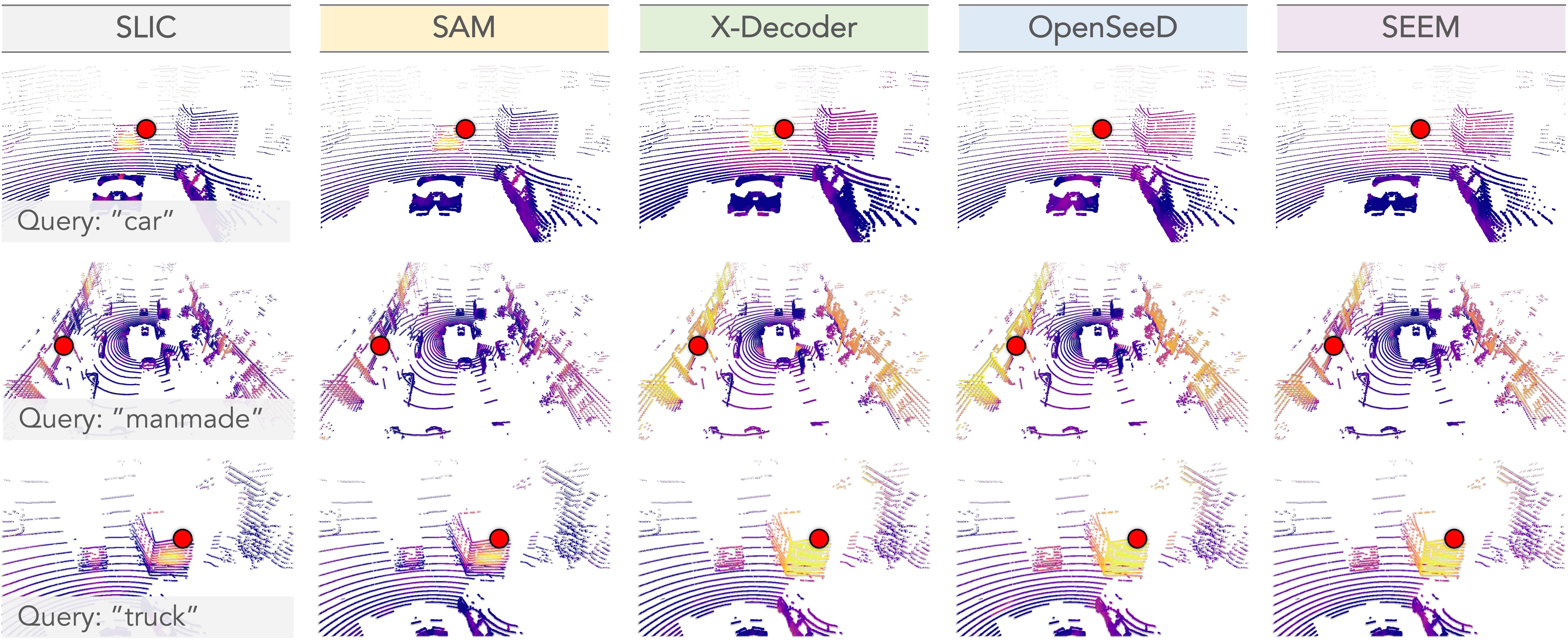
Figure 5: The cosine similarity between a query point (denoted as the red dot) and the feature learned with SLIC [29] and different VFMs [6, 7, 26, 8]. The queried semantic classes from top to bottom examples are: “car”, “manmade”, and “truck”. The color goes from violet to yellow denoting low and high similarity scores, respectively. Best viewed in colors.

4.4 Multi-Source Data Pretraining

Previous works [27, 28] predominantly focus on pretraining models with single-source LiDAR datasets. This approach limits their generalization capability when applied to out-of-source tasks, as different LiDAR datasets often exhibit diverse characteristics, such as varying sparsity, intensity ranges, and other sensor-specific attributes. To overcome these limitations, we propose a multi-source data pretraining strategy that integrates diverse datasets, improving the robustness of feature representations. This strategy enhances the model’s adaptability to different LiDAR sensors and boosts its generalization performance across domains.

Multi-Source Contrastive Learning. Consider multiple LiDAR datasets $\{\{\mathcal{P}^{(i)};\mathcal{I}^{(i)}\}\mid i=1,\ldots,S\}$ from $S$ distinct sources. Our LiDAR point cloud network $F_{\theta_{p}}$ is designed to perform consistently across all sensors. However, significant discrepancies exist in the feature distributions of these datasets. For instance, intensity values in nuScenes [111], range from $0$ to $255$; whereas the intensity values in SemanticKITTI  [112] range from $0$ to $1$. These differences complicate the learning process when using shared model weights across datasets.

To address these domain-specific variations, we first normalize the feature embeddings for each data source. For each dataset, we compute the mean $\epsilon^{(i)}$ and variance $\sigma^{(i)}$ of the feature distributions, then normalize the feature embeddings as follows:

$$\hat{e}^{(i)}_{j}=\frac{e^{(i)}_{j}-\epsilon^{(i)}}{\sigma^{(i)}}.$$ (6)

This normalization ensures consistent feature representation across datasets, minimizing the impact of differing distribution characteristics. After normalization, the feature embeddings are fed into the network $F_{\theta_{p}}$, which generates point features that are grouped into superpoint embeddings, $\{\mathbf{K}^{(i)}\mid i=1,\dots,S\}$, for each domain.

To improve the model’s generalizability across datasets, we employ a cross-dataset pretraining contrastive loss $\mathcal{L}^{\text{cdp}}$, which encourages the model to learn shared representations across data sources while preserving the unique characteristics of each domain. This loss is defined as follows:

$$-\frac{1}{M}{\sum_{i=1}^{M}\log\left[\frac{e^{\left(\left<\mathbf{k}^{(m)}_{i},\mathbf{k}^{(n)}_{i}\right>/\tau\right)}}{\sum_{j\neq i}e^{\left(\left<\mathbf{k}^{(m)}_{i},\mathbf{k}^{(n)}_{j}\right>/\tau\right)}+e^{\left(\left<\mathbf{k}^{(m)}_{i},\mathbf{k}^{(n)}_{i}\right>/\tau\right)}}\right]}~.$$ (7)

Here, this loss ensures that superpoint embeddings from the same source are more similar, while simultaneously maintaining sufficient separation between superpoints from different sources. This contrastive objective strengthens the model’s ability to handle data from multiple domains and encourages the development of shared, yet adaptable, feature representations.

The multi-source data pretraining leverages a variety of data sources to create a more resilient and flexible model. By addressing the substantial distributional differences between domains, feature normalization ensures consistency across diverse datasets, facilitating a more unified representation space. The cross-source contrastive loss further enhances adaptability, enabling it to transfer knowledge across multiple domains while maintaining domain-specific distinctions. As we will show in Sec. 5, this strategy results in improved generalization across different LiDAR sensors, leading to stronger performance on out-of-source downstream tasks.

TABLE I: Benchmark study of data pretraining methods that are pretrained on nuScenes [118] and fine-tuned on nuScenes [111], SemanticKITTI [112], and Waymo Open [113]. The evaluations are conducted on the official validation split of each dataset. Group (a): random initialization. Group (b): single-modality data pretraining. Group (c): image-to-LiDAR data pretraining by distilling ResNet [119]. Groups (d), (e), and (f): image-to-LiDAR data pretraining by distilling ViT [120] (Small, Medium, Large) from DINOv2 [71]. LP denotes linear probing with frozen backbones. All mIoU scores are given in percentage (%). The best and second best scores under each group are highlighted in bold and underline.

#	Method	Venue	Backbone	Backbone	nuScenes						KITTI	Waymo
			(2D)	(3D)	LP	1%	5%	10%	25%	Full	1%	1%
(a)	Random	-	-	MinkU-34	8.10	30.30	47.84	56.15	65.48	74.66	39.50	39.41
(b)	PointContrast [102]	ECCV’20	-	MinkU-34	21.90	32.50	-	-	-	-	41.10	-
	DepthContrast [103]	ICCV’21	-	MinkU-34	22.10	31.70	-	-	-	-	41.50	-
	ALSO [100]	CVPR’23	-	MinkU-34	-	37.70	-	59.40	-	72.00	-	-
	BEVContrast [101]	3DV’24	-	MinkU-34	-	38.30	-	59.60	-	72.30	-	-
(c)	PPKT [114]	arXiv’21	ResNet-50	MinkU-34	35.90	37.80	53.74	60.25	67.14	74.52	44.00	47.60
	SLidR [27]	CVPR’22	ResNet-50	MinkU-34	38.80	38.30	52.49	59.84	66.91	74.79	44.60	47.12
	ST-SLidR [28]	CVPR’23	ResNet-50	MinkU-34	40.48	40.75	54.69	60.75	67.70	75.14	44.72	44.93
	TriCC [121]	CVPR’23	ResNet-50	MinkU-34	38.00	41.20	54.10	60.40	67.60	75.60	45.90	-
	Seal [9]	NeurIPS’23	ResNet-50	MinkU-34	44.95	45.84	55.64	62.97	68.41	75.60	46.63	49.34
	CSC [122]	CVPR’24	ResNet-50	MinkU-34	46.00	47.00	57.00	63.30	68.60	75.70	47.20	-
	HVDistill [123]	IJCV’24	ResNet-50	MinkU-34	39.50	42.70	56.60	62.90	69.30	76.60	49.70	-
	LargeAD	Ours	ResNet-50	MinkU-34	46.13	47.08	56.90	63.74	69.34	76.03	49.55	50.29
(d)	PPKT [114]	arXiv’21	ViT-S	MinkU-34	38.60	40.60	52.06	59.99	65.76	73.97	43.25	47.44
	SLidR [27]	CVPR’22	ViT-S	MinkU-34	44.70	41.16	53.65	61.47	66.71	74.20	44.67	47.57
	Seal [9]	NeurIPS’23	ViT-S	MinkU-34	45.16	44.27	55.13	62.46	67.64	75.58	46.51	48.67
	ScaLR [124]	CVPR’24	ViT-S	MinkU-34	42.40	40.50	-	-	-	-	-	-
	LargeAD	Ours	ViT-S	MinkU-34	46.58	46.78	57.33	63.85	68.66	75.75	50.07	50.83
(e)	PPKT [114]	arXiv’21	ViT-B	MinkU-34	39.95	40.91	53.21	60.87	66.22	74.07	44.09	47.57
	SLidR [27]	CVPR’22	ViT-B	MinkU-34	45.35	41.64	55.83	62.68	67.61	74.98	45.50	48.32
	Seal [9]	NeurIPS’23	ViT-B	MinkU-34	46.59	45.98	57.15	62.79	68.18	75.41	47.24	48.91
	LargeAD	Ours	ViT-B	MinkU-34	47.84	48.37	59.36	64.11	69.02	75.91	50.68	51.52
(f)	PPKT [114]	arXiv’21	ViT-L	MinkU-34	41.57	42.05	55.75	61.26	66.88	74.33	45.87	47.82
	SLidR [27]	CVPR’22	ViT-L	MinkU-34	45.70	42.77	57.45	63.20	68.13	75.51	47.01	48.60
	Seal [9]	NeurIPS’23	ViT-L	MinkU-34	46.81	46.27	58.14	63.27	68.67	75.66	47.55	50.02
	LargeAD	Ours	ViT-L	MinkU-34	48.71	49.21	60.37	64.82	69.85	75.94	51.68	52.68

4.5 Overall Framework

Our framework integrates several innovative components to achieve scalable and robust 3D scene understanding. A key element is the use of VFMs to generate semantically enriched superpixels, addressing issues like over-segmentation and self-conflict in traditional methods. This enables better alignment between 2D image features and 3D LiDAR data, enhancing overall representation learning.

Our method incorporates the VFM-assisted contrastive loss $\mathcal{L}^{\text{vfm}}$, ensuring semantic coherence between superpixels and superpoints, while the temporal consistency loss $\mathcal{L}^{\text{tmp}}$ maintains stable point representations across frames. The point-to-segment regularization loss $\mathcal{L}^{\text{p2s}}$ further improves spatial coherence within segments. Finally, the cross-dataset pretraining loss $\mathcal{L}^{\text{cdp}}$ addresses domain-specific variations, enhancing the model’s ability to generalize across different LiDAR sensors. Together, these objectives create a robust and versatile framework, ensuring superior performance across various tasks and domains while maintaining scalability and adaptability in real-world applications.

5 Experiments

In this section, we conduct extensive experiments to validate the effectiveness of the proposed LargeAD framework. We first introduce the datasets (Sec. 5.1) and describe the implementation details (Sec. 5.2). Next, we present a comparative study, demonstrating the superior performance of our framework compared to state-of-the-art methods across multiple tasks and datasets (Sec. 5.3). Finally, we provide an in-depth ablation study to analyze the impact of different components and data sources on the performance (Sec. 5.4).

5.1 Datasets

We evaluate the effectiveness of our approach using eleven diverse datasets. The first group includes large-scale real-world LiDAR datasets: ¹nuScenes [111, 118], ²SemanticKITTI [112], and ³Waymo Open [113]. These datasets capture urban driving scenes, with nuScenes utilizing a Velodyne HDL32E sensor, while SemanticKITTI and Waymo Open use 64-beam LiDARs. We also include ⁴ScribbleKITTI [17], which shares data with SemanticKITTI but offers weak annotations in the form of line scribbles. For off-road scenarios, we consider ⁵RELLIS-3D [125], which contains multimodal data from a campus environment, and ⁶SemanticPOSS [126], a smaller dataset with a focus on dynamic objects. Additionally, we incorporate ⁷SemanticSTF [127], which provides LiDAR scans collected in adverse weather conditions. Three synthetic datasets are also utilized: ⁸SynLiDAR [128], ⁹Synth4D [67], and ¹⁰DAPS-3D [129], all generated using simulators to provide diverse driving environments and scenarios. Finally, we assess robustness on ¹¹nuScenes-C [130], a benchmark from the Robo3D challenge featuring eight out-of-distribution corruptions common in real-world driving. For further details, we refer readers to the respective publications associated with each dataset.

TABLE II: Benchmark study of data pretraining methods that are: (a) random initialized, (b) pretrained on SemanticKITTI [112], (c) pretrained on Waymo Open [113], and (d) pretrained based on the proposed large-scale cross-sensor data pretraining pipeline. After pretraining, all methods are fine-tuned on SemanticKITTI [112], nuScenes [111], and Waymo Open [113], respectively, and evaluated on the official validation split of each dataset. LP denotes linear probing with frozen backbones. All mIoU scores are given in percentage (%). The best and second best scores are highlighted in bold and underline.

#	Method	Venue	Distill	SemanticKITTI				nuScenes				Waymo
				LP	1%	10%	Full	LP	1%	10%	Full	LP	1%	10%	Full
(a)	Random	-	-	7.45	39.50	55.11	57.39	8.10	30.30	56.15	74.66	6.45	39.41	59.71	64.22
(b)	SLidR [27]	CVPR’22	ViT-B	32.83	45.20	56.18	56.60	16.54	35.21	56.77	74.47	27.82	44.35	60.55	64.33
	Seal [9]	NeurIPS’23	ViT-B	33.46	47.52	57.68	58.64	18.18	38.86	58.05	74.53	29.36	45.96	61.59	64.81
(c)	SLidR [27]	CVPR’22	ViT-B	32.29	44.75	55.66	57.49	23.97	39.16	58.47	73.96	32.21	47.96	61.33	64.43
	Seal [9]	NeurIPS’23	ViT-B	33.21	47.46	57.61	58.72	25.74	42.69	60.59	74.38	34.65	49.30	62.37	65.79
(d)	LargeAD	Ours	ViT-B	35.77	50.68	60.18	60.98	47.84	48.37	64.11	75.91	36.12	51.52	63.92	66.10

TABLE III: Comparisons of different data pretraining methods that are: (a) random initialized, (b) pretrained on nuScenes [118], (c) pretrained on SemanticKITTI [112], (d) pretrained on Waymo Open [113], and (e) pretrained based on the proposed large-scale cross-sensor data pretraining pipeline. After pretraining, all methods are fine-tuned on different downstream datasets [17, 125, 126, 127, 128, 129, 67], respectively, and evaluated on the official validation split of each dataset. All mIoU scores are given in percentage (%). The best and second best scores are highlighted in bold and underline.

#	Method	ScribbleKITTI		RELLIS-3D		SemanticPOSS		SemanticSTF		SynLiDAR		DAPS-3D		Synth4D
		1%	10%	1%	10%	Half	Full	Half	Full	1%	10%	Half	Full	1%	10%
(a)	Random	23.81	47.60	38.46	53.60	46.26	54.12	48.03	48.15	19.89	44.74	74.32	79.38	20.22	66.87
(b)	PPKT [114]	36.50	51.67	49.71	54.33	50.18	56.00	50.92	54.69	37.57	46.48	78.90	84.00	61.10	62.41
	SLidR [27]	39.60	50.45	49.75	54.57	51.56	55.36	52.01	54.35	42.05	47.84	81.00	85.40	63.10	62.67
	Seal [9]	40.64	52.77	51.09	55.03	53.26	56.89	53.46	55.36	43.58	49.26	81.88	85.90	64.50	66.96
(c)	SLidR [27]	40.27	51.92	47.65	54.03	49.97	54.83	51.39	53.83	40.11	43.90	74.93	80.31	57.24	61.25
	Seal [9]	41.97	53.25	49.23	54.93	52.31	55.47	53.26	55.49	41.48	45.52	76.31	81.24	59.25	64.21
(d)	SLidR [27]	38.24	48.96	47.31	53.20	50.93	55.04	50.93	54.35	43.91	49.32	79.02	84.34	61.98	62.15
	Seal [9]	39.13	50.53	50.55	54.68	52.90	55.27	52.20	55.24	44.78	50.98	79.68	84.68	63.74	65.39
(e)	LargeAD	43.45	54.62	53.31	56.62	54.47	57.11	55.14	56.89	47.12	52.82	83.31	86.21	65.33	67.12

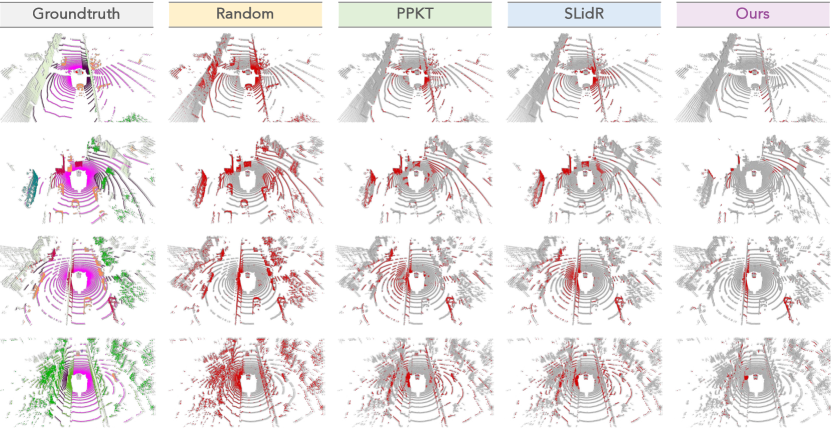
Figure 6: The qualitative results of random initialization and different image-to-LiDAR data pretraining approaches [114, 27] pretrained and fine-tuned (with $1\%$ labeled data) on nuScenes [118]. To highlight the differences, the correct / incorrect predictions are painted in gray / red, respectively. Best viewed in colors and zoomed-in for additional details.

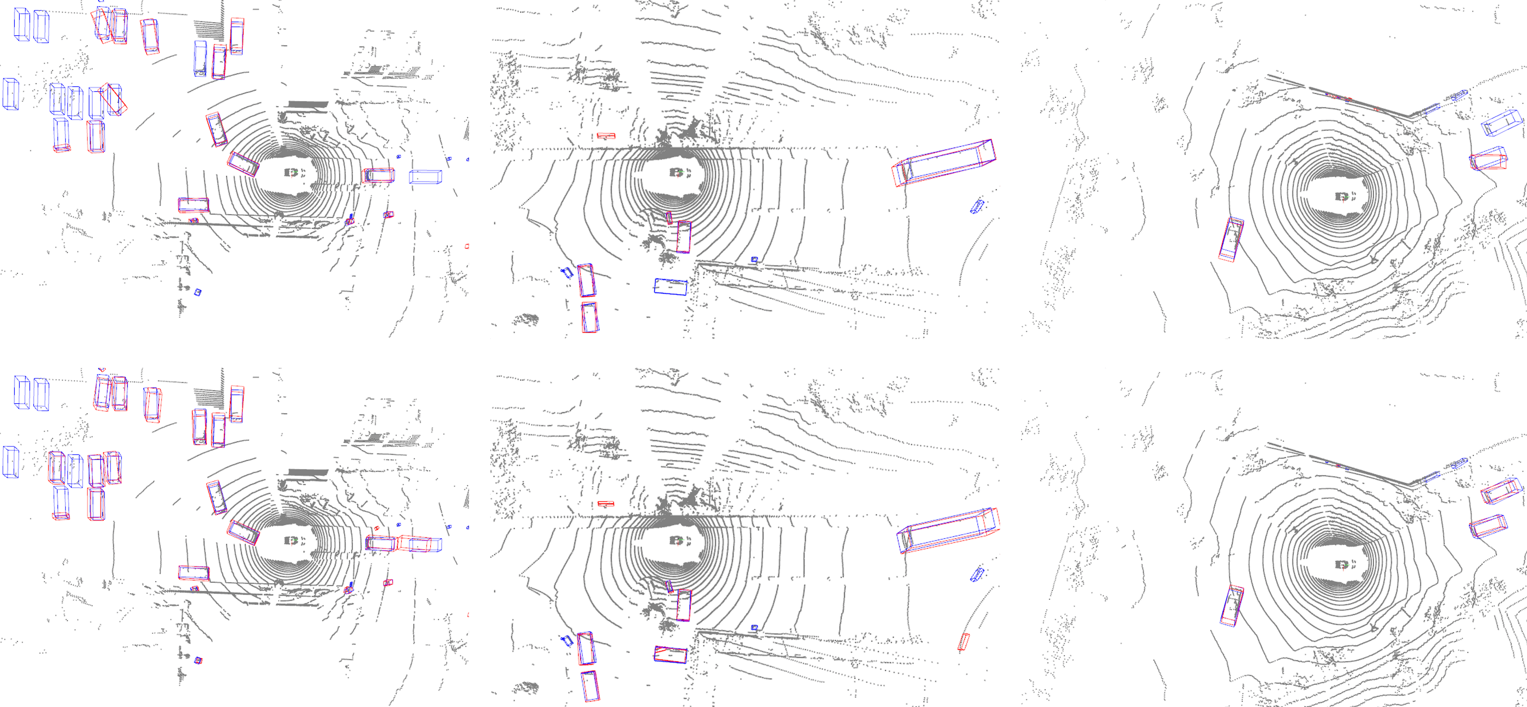
Figure 7: The qualitative results of object detection trained with $5\%$ labeled data. The first row shows the model trained with random initialization, while the second row displays results from our proposed framework. The groundtruth / predicted results are highlighted with blue / red boxes, respectively. Best viewed in colors and zoomed-in for additional details.

TABLE IV: Robustness probing of data pretraining methods under eight out-of-distribution corruptions in the nuScenes-C dataset from the Robo3D benchmark [130]. The mCE score is the lower the better while mRR and mIoU scores are the higher the better. All mCE, mRR, and mIoU scores are given in percentage (%). Avg denotes the average mIoU scores of methods across all eight corruptions. The best and second best scores are highlighted in bold and underline.

#	Initial	Backbone	mCE	mRR	Fog	Wet	Snow	Move	Beam	Cross	Echo	Sensor	Avg
LP	PPKT [114]	MinkU-34	183.44	78.15	30.65	35.42	28.12	29.21	32.82	19.52	28.01	20.71	28.06
	SLidR [27]	MinkU-34	179.38	77.18	34.88	38.09	32.64	26.44	33.73	20.81	31.54	21.44	29.95
	Seal [9]	MinkU-34	166.18	75.38	37.33	42.77	29.93	37.73	40.32	20.31	37.73	24.94	33.88
	LargeAD	MinkU-34	160.28	77.29	40.54	43.26	37.92	38.27	40.27	25.67	39.26	30.62	36.98
Full	Random	PolarNet	115.09	76.34	58.23	69.91	64.82	44.60	61.91	40.77	53.64	42.01	54.49
	Random	CENet	112.79	76.04	67.01	69.87	61.64	58.31	49.97	60.89	53.31	24.78	55.72
	Random	WaffleIron	106.73	72.78	56.07	73.93	49.59	59.46	65.19	33.12	61.51	44.01	55.36
	Random	Cylinder3D	105.56	78.08	61.42	71.02	58.40	56.02	64.15	45.36	59.97	43.03	57.42
	Random	SPVCNN-34	106.65	74.70	59.01	72.46	41.08	58.36	65.36	36.83	62.29	49.21	55.58
	Random	MinkU-34	112.20	72.57	62.96	70.65	55.48	51.71	62.01	31.56	59.64	39.41	54.18
	PPKT [114]	MinkU-34	105.64	76.06	64.01	72.18	59.08	57.17	63.88	36.34	60.59	39.57	56.60
	SLidR [27]	MinkU-34	106.08	75.99	65.41	72.31	56.01	56.07	62.87	41.94	61.16	38.90	56.83
	Seal [9]	MinkU-34	92.63	83.08	72.66	74.31	66.22	66.14	65.96	57.44	59.87	39.85	62.81
	LargeAD	MinkU-34	91.75	83.61	71.95	72.47	67.28	65.29	67.49	59.42	61.38	42.46	63.47

TABLE V: Comparisons of state-of-the-art pretraining methods pretrained and fine-tuned on nuScenes [111] using the specified data proportions. All methods employ CenterPoint [131] or SECOND [132] as the 3D object detection backbones. All sores are given in percentage (%). The best and second best scores are highlighted in bold and underline.

Method	nuScenes
	5%		10%		20%
	mAP	NDS	mAP	NDS	mAP	NDS
Backbone: VoxelNet + CenterPoint
Random	38.0	44.3	46.9	55.5	50.2	59.7
PointContrast [102]	39.8	45.1	47.7	56.0	-	-
GCC-3D [133]	41.1	46.8	48.4	56.7	-	-
SLidR [27]	43.3	52.4	47.5	56.8	50.4	59.9
TriCC [121]	44.6	54.4	48.9	58.1	50.9	60.3
Seal [9]	44.7	54.0	49.0	58.1	51.4	60.7
CSC [122]	45.3	54.2	49.3	58.3	51.9	61.3
LargeAD	45.8	54.6	49.7	58.8	52.1	61.4
Backbone: VoxelNet + SECOND
Random	35.8	45.9	39.0	51.2	43.1	55.7
SLidR [27]	36.6	48.1	39.8	52.1	44.2	56.3
TriCC [121]	37.8	50.0	41.4	53.5	45.5	57.7
Seal [9]	37.9	49.4	41.9	54.0	44.9	57.4
CSC [122]	38.2	49.4	42.5	54.8	45.6	58.1
LargeAD	38.3	49.9	43.0	55.0	45.7	58.7

TABLE VI: Ablation study on the knowledge transfer effects from the classic SLIC [29] algorithm and different vision foundation models [6, 7, 26, 8]. Both SLidR [27] and our framework are pretrained on nuScenes [118] and fine-tuned on nuScenes [111], SemanticKITTI [112], Waymo Open [113], SemanticPOSS [126], SemanticSTF [134], and Synth4D [67], respectively, and evaluated on the official validation split of each dataset. LP denotes linear probing with frozen backbones. All mIoU scores are given in percentage (%). The best and second best scores are highlighted in bold and underline.

Method	Superpixel	nuScenes						KITTI	Waymo	POSS	STF	Syn4D
		LP	1%	5%	10%	25%	Full	1%	1%	Half	Half	1%
Random	-	8.10	30.30	47.84	56.15	65.48	74.66	39.50	39.41	46.26	48.03	20.22
SLidR	SLIC [29]	38.80	38.30	52.49	59.84	66.91	74.79	44.60	47.12	51.56	52.01	63.10
	SAM [6]	41.49	43.67	55.97	61.74	68.85	75.40	43.35	48.64	51.37	52.12	63.15
	X-Decoder [7]	41.71	43.02	54.24	61.32	67.35	75.11	45.70	48.73	51.50	52.28	63.21
	OpenSeeD [26]	42.61	43.82	54.17	61.03	67.30	74.85	45.88	48.64	52.09	52.37	63.31
	SEEM [8]	43.00	44.02	53.03	60.84	67.38	75.21	45.72	48.75	52.00	52.36	63.13
Ours	SLIC [29]	40.89	39.77	53.33	61.58	67.78	75.32	45.75	47.74	52.77	52.91	63.37
	SAM [6]	43.94	45.09	56.95	62.35	69.08	75.92	46.53	49.00	53.21	53.37	63.76
	X-Decoder [7]	42.64	44.31	55.18	62.03	68.24	75.56	46.02	49.11	53.17	53.40	64.21
	OpenSeeD [26]	44.67	44.74	55.13	62.36	69.00	75.64	46.13	48.98	53.01	53.27	64.29
	SEEM [8]	44.95	45.84	55.64	62.97	68.41	75.60	46.63	49.34	53.26	53.46	64.50

TABLE VII: Ablation study of each component in our framework. All variants are pretrained on nuScenes [118] and fine-tuned on nuScenes [118], SemanticKITTI [112], and Waymo Open [113], respectively. The knowledge is distilled from the ResNet-50. C2L: Camera-to-LiDAR distillation. VFM: Vision foundation models. STC: Superpoint temporal consistency. P2S: Point-to-segment regularization. CDP: Cross-dataset pretraining. LP denotes linear probing with frozen backbones. All mIoU scores are given in percentage (%). The best and second best scores are highlighted in bold and underline.

#	C2L	VFM	STC	P2S	CDP	nuScenes						KITTI	Waymo
						LP	1%	5%	10%	25%	Full	1%	1%
(a)	✓					38.80	38.30	52.49	59.84	66.91	74.79	44.60	47.12
(b)	✓		✓			40.45	41.62	54.67	60.48	67.61	75.30	45.38	48.08
(c)	✓	✓				43.00	44.02	53.03	60.84	67.38	75.21	45.72	48.75
(d)	✓	✓	✓			44.01	44.78	55.36	61.99	67.70	75.00	46.49	49.15
(e)	✓	✓		✓		43.35	44.25	53.69	61.11	67.42	75.44	46.07	48.82
(f)	✓	✓	✓	✓		44.95	45.84	55.64	62.97	68.41	75.60	46.63	49.34
(g)	✓	✓	✓	✓	✓	46.13	47.08	56.90	63.74	69.34	76.03	49.55	50.29

TABLE VIII: Ablation study on the utilization of multiple data sources during pretraining. The knowledge is distilled from the ViT-B. N, K, and W denote pretraining on nuScenes [118], SemanticKITTI [112], and Waymo Open [113], respectively. LP denotes linear probing with frozen backbones. All mIoU scores are given in percentage (%). The best and second best scores are highlighted in bold and underline.

N	K	W	nuScenes		KITTI		Waymo
			LP	1%	LP	1%	LP	1%
			8.10	30.30	7.45	39.50	6.45	39.41
✓			46.59	45.98	29.25	47.24	32.42	48.91
	✓		18.18	38.86	33.46	47.52	29.36	45.96
		✓	25.74	42.69	33.21	47.46	34.65	49.30
✓	✓		47.19	47.80	34.09	49.12	31.34	50.00
✓		✓	47.42	47.94	33.16	48.61	35.84	50.81
	✓	✓	31.08	44.77	34.67	50.16	35.49	50.96
✓	✓	✓	47.84	48.37	35.77	50.68	36.12	51.52

5.2 Implementation Details

We utilize MinkUNet [45] as our 3D backbone, processing cylindrical voxels with a resolution of $0.10$m. For the 2D backbone, we adopt models from ResNet-50 [119] and the ViT family [120], pretrained using the DINOv2 framework [71], as proposed in [124]. The pretraining of our LiDAR point cloud encoder spans 50 epochs, using eight GPUs with a batch size of 32. We employ AdamW for optimization, coupled with a OneCycle learning rate scheduler. During fine-tuning, we strictly adhere to the data splits, augmentation strategies, and evaluation protocols from SLidR [27] for the nuScenes and SemanticKITTI datasets, extending similar procedures to other datasets. The training objective combines cross-entropy loss and Lovász-Softmax loss [135] to optimize the model. For multi-source data pretraining, we combine data from three major datasets: nuScenes, SemanticKITTI, and Waymo Open. We also study the impact of pretraining with each of and the combination of these three dataset. Image-LiDAR pairs from these datasets are randomly sampled to form the training batches. We report results of prior works based on their official publications [27, 28]. Additionally, for methods like PPKT [114] and SLidR [27], which were only evaluated on nuScenes and SemanticKITTI, we reproduce their performance on the other nine datasets using publicly available code.

Evaluation Metrics. For linear probing and downstream tasks on LiDAR semantic segmentation, we report the Intersection-over-Union (IoU) for each semantic class and the mean IoU (mIoU) across all classes. For 3D object detection, we report the mean Average Precision (mAP) and nuScenes Detection Score (NDS). For robustness evaluation, we follow the Robo3D protocol [130] and report the mean Corruption Error (mCE) and mean Resilience Rate (mRR) scores. The baseline model used for these evaluations is the MinkUNet implementation by Tang et al. [51].

5.3 Comparative Study

Comparisons to State-of-the-Arts. We compare the proposed LargeAD against random initialization and a total of eleven state-of-the-art pretraining techniques using both linear probing (LP) and few-shot fine-tuning protocols on nuScenes [118], as presented in Tab. I. The results demonstrate the significant impact of pretraining on downstream task performance, particularly in low-data regimes such as $1\%$, $5\%$, and $10\%$ fine-tuning budgets. When distilling the knowledge from ResNet, ViT-S, ViT-B, and ViT-L, our framework achieves mIoU scores of $46.13\%$, $46.58\%$, $47.84\%$, and $48.71\%$ under the LP setting, outperforming the previous best models [28, 9, 122, 124] by large margins. Moreover, our framework consistently delivers the highest performance across almost all fine-tuning tasks on nuScenes, highlighting the effectiveness of VFM-assisted contrastive learning, the incorporation of spatial-temporal consistency regularization, and the combination of multi-source data pretraining.

Downstream Generalization. To thoroughly evaluate the generalization capability of LargeAD, we perform experiments across a total of nine autonomous driving datasets, with the results summarized in Tab. I (for SemanticKITTI and Waymo Open) and Tab. III (for the other seven datasets). Each dataset presents distinct challenges, including variations in sensor types, acquisition environments, scale, and data fidelity, making this a rigorous assessment of model generalization. Our framework achieves $51.68\%$ and $52.68\%$ mIoU scores on SemanticKITTI and Waymo Open when distilling from ViT-L, setting new states for these benchmarks. We also surpass SLidR [27] and Seal [9] on the other seven datasets, as shown in Tab. III. The results consistently show that the proposed method outperforms existing state-of-the-art approaches on all evaluated datasets. These outcomes underline the robustness and adaptability of our proposed approach to a wide range of real-world automotive perception tasks.

Robustness Probing. Assessing the robustness of learned representations on out-of-distribution data is crucial, particularly for real-world applications where environments are unpredictable. We utilize the nuScenes-C dataset from the Robo3D benchmark [130] to evaluate robustness under various corruptions. As shown in Tab. IV, self-supervised learning methods like PPKT [114] and SLidR [27] generally demonstrate better resilience compared to traditional baselines (with the random initialization) such as MinkUNet [45]. Our approach, LargeAD, achieves superior robustness across nearly all corruption types, outperforming other recent segmentation backbones that rely on different LiDAR representations, including range view [40], bird’s eye view (BEV) [43], raw point-based methods [35], and multi-view fusion [51]. These results underscore the adaptability and resilience of our pretraining framework under diverse real-world autonomous driving conditions.

Enhancements for 3D Object Detection. In addition to LiDAR semantic segmentation, we extend our framework to 3D object detection tasks on the nuScenes dataset [111] and compare it with state-of-the-art pretraining methods. The results, shown in Tab. V, indicate that LargeAD consistently outperforms competing approaches across various data proportions ($5\%$, $10\%$, and $20\%$) for both the CenterPoint [131] and SECOND [132] backbones. In particular, our method achieves the highest mAP and NDS at all fine-tuning levels, surpassing recent techniques such as CSC [122] and TriCC [121]. Notably, our framework maintains superior performance with limited fine-tuning data, demonstrating its robustness and effectiveness for 3D object detection. These results further validate the generalizability of our framework across multiple challenging tasks in autonomous driving, from semantic segmentation to object detection.

Qualitative Assessment. To further assess the performance of our framework, we visualize the segmentation predictions on nuScenes [118] in Fig. 6. The pretraining methods clearly enhance segmentation quality compared to models trained from random initialization. Among the compared approaches, LargeAD demonstrates the most consistent and accurate results, particularly in complex driving environments. This improvement can be attributed to the robust spatial and temporal consistency learning embedded in our pretraining strategy. Additionally, we perform qualitative comparisons of our framework with the random initialization on the 3D object detection. Qualitative results from Fig. 7 further highlight our superiority. Our framework generates significantly more accurate predictions, closely matching ground truth boxes and outperforming models trained from random initialization, which exhibit greater inaccuracies. The strong performance across both tasks underscores the generalizability and robustness of our pretraining approach.

5.4 Ablation Study

Comparing Different Foundation Models. This study serves as the first attempt of adapting VFMs for large-scale point cloud representation learning. We conduct a comprehensive ablation study on four popular VFMs, i.e., SAM [6], X-Decoder [7], OpenSeeD [26], and SEEM [8], and show the results in Tab. VI. Our experiments reveal that different VFMs have varying levels of impact on contrastive learning objectives. All VFMs consistently outperform traditional SLIC [29] when integrated into both frameworks. SEEM [8] emerges as the top performer, providing the most consistent improvements. Interestingly, SAM [6] generates more fine-grained superpixels, which enhances performance when fine-tuning with larger labeled datasets. We hypothesize that SAM [6] offers more diverse negative samples, which may benefit the superpixel-driven contrastive learning. Across all configurations, LargeAD surpasses SLidR [27] by a significant margin, affirming the effectiveness of our proposed large-scale cross-sensor data pretraining framework.

Cosine Similarity. We visualize feature similarities across various VFMs in Fig. 5, providing insights into the distinction in representations even before fine-tuning. Semantically enriched models like X-Decoder [7], OpenSeeD [26], and SEEM [8] exhibit clear feature distinctions between objects and backgrounds. In contrast, unsupervised or overly fine-grained methods such as SLIC [29] and SAM [6] show weaker semantic awareness. These qualitative observations are mirrored in the performance results from both linear probing and fine-tuning tasks (see Tab. VI), where SEEM demonstrates stronger consistency regularization during cross-sensor representation learning, leading to improved downstream task performance.

Component Analysis. The ablation results of the core components of LargeAD are provided in Tab. VII. Integrating VFMs alone (row c) delivers a $4.20\%$ mIoU improvement in linear probing, while adding temporal consistency learning (row b) yields an additional $1.65\%$ mIoU gain. Combining these two components (row d) results in a total of $5.21\%$ mIoU boost. The point-to-segment regularization (row e) also contributes a significant improvement of $4.55\%$ mIoU on its own. When all components are integrated (row g), the final model achieves a total $6.33\%$ mIoU gain over SLidR [27], outperforming all state-of-the-art methods on both in-distribution and out-of-distribution benchmarks.

Scaling with Data Sources. We conduct an ablation study to examine the impact of using different datasets during pretraining, as summarized in Tab. VIII. The results demonstrate that pretraining on a single dataset, i.e., nuScenes (N) [118], SemanticKITTI (K) [112], or Waymo Open (W) [113], provides notable improvements over random initialization, especially in the linear probing (LP) and $1\%$ fine-tuning evaluations. However, as more datasets are combined during pretraining, the performance continues to improve consistently across both in-domain (the pretrained dataset) and out-of-domain datasets. For example, pretraining on all three datasets (N + K + W) results in the best performance, achieving a significant boost across all scenarios. Interestingly, the benefits of multi-dataset pretraining are most evident in the out-of-domain results, where combining two or three datasets leads to substantial gains over single-dataset pretraining. For instance, the inclusion of both nuScenes and Waymo Open (N + W) leads to a $47.42\%$ mIoU in LP on nuScenes, outperforming the single-dataset pretraining setups. Similarly, using all three datasets outperforms two-dataset combinations in both LP and fine-tuning, particularly in out-of-domain scenarios like Waymo Open, where it achieves a remarkable $51.52\%$ mIoU in $1\%$ fine-tuning. These results highlight the importance of multi-source pretraining, which not only improves generalization within in-domain datasets but also significantly enhances out-of-domain performance, showcasing the robustness and scalability of our proposed framework.

6 Conclusion

In this paper, we introduced LargeAD, a scalable and generalizable framework designed for large-scale pretraining across diverse LiDAR datasets. Our approach leverages vision foundation models (VFMs) to generate semantically enriched superpixels, aligning 2D image features with LiDAR point clouds for improved representation learning. By integrating VFM-assisted contrastive learning, superpoint temporal consistency, and multi-source data pretraining, our framework achieves state-of-the-art performance on multiple 3D scene understanding tasks, including LiDAR-based semantic segmentation and 3D object detection. Extensive experiments conducted on eleven diverse datasets highlight the effectiveness of our framework in both in-domain and out-of-domain scenarios. Our framework not only excels in downstream generalization but also demonstrates superior robustness under out-of-distribution conditions. The ablation study further validates the importance of our design choices, showcasing the significant impact of incorporating multiple datasets during pretraining and the benefits of each individual component of our framework. The results underline the potential of LargeAD to advance real-world autonomous driving applications by providing a more versatile and resilient model capable of adapting to various sensor configurations and driving environments. In future work, we aim to extend our approach to incorporate additional sensor modalities, such as radar and thermal imaging, further broadening the scope of cross-modal pretraining for autonomous systems.

Acknowledgments. This work is supported by the Ministry of Education, Singapore, under its MOE AcRF Tier 2 (MOET2EP20221- 0012), NTU NAP, and under the RIE2020 Industry Alignment Fund – Industry Collaboration Projects (IAF-ICP) Funding Initiative, as well as cash and in-kind contribution from the industry partner(s).

References

- [1] M. Shoeybi, M. Patwary, R. Puri, P. LeGresley, J. Casper, and B. Catanzaro, “Megatron-lm: Training multi-billion parameter language models using model parallelism,” arXiv preprint arXiv:1909.08053, 2019.
- [2] J. Hoffmann, S. Borgeaud, A. Mensch, E. Buchatskaya, and et al., “Training compute-optimal large language models,” in Adv. Neural Inf. Process. Syst., vol. 35, 2022, pp. 30 016–30 030.
- [3] S. Zhang, S. Roller, N. Goyal, M. Artetxe, and et al., “Opt: Open pre-trained transformer language models,” arXiv preprint arXiv:2205.01068, 2022.
- [4] OpenAI, “Gpt-4 technical report,” arXiv preprint arXiv:2303.08774, 2023.
- [5] A. Chowdhery, S. Narang, J. Devlin, M. Bosma, G. Mishra, A. Roberts, P. Barham, and et al., “Palm: Scaling language modeling with pathways,” J. Mach. Learn. Research, vol. 24, no. 240, pp. 1–113, 2023.
- [6] A. Kirillov, E. Mintun, N. Ravi, H. Mao, C. Rolland, L. Gustafson, T. Xiao, S. Whitehead, A. C. Berg, W.-Y. Lo, P. Dollár, and R. Girshick, “Segment anything,” in IEEE/CVF Int. Conf. Comput. Vis., 2023, pp. 4015–4026.
- [7] X. Zou, Z.-Y. Dou, J. Yang, Z. Gan, and et al., “Generalized decoding for pixel, image, and language,” in IEEE/CVF Conf. Comput. Vis. Pattern Recog., 2023, pp. 15 116–15 127.
- [8] X. Zou, J. Yang, H. Zhang, F. Li, L. Li, J. Gao, and Y. J. Lee, “Segment everything everywhere all at once,” in Adv. Neural Inf. Process. Syst., vol. 36, 2023, pp. 19 769–19 782.
- [9] Y. Liu, L. Kong, J. Cen, R. Chen, W. Zhang, L. Pan, K. Chen, and Z. Liu, “Segment any point cloud sequences by distilling vision foundation models,” in Adv. Neural Inf. Process. Syst., vol. 36, 2023, pp. 37 193–37 229.
- [10] R. Li, S. Li, L. Kong, X. Yang, and J. Liang, “Seeground: See and ground for zero-shot open-vocabulary 3d visual grounding,” arXiv preprint arXiv:2412.04383, 2024.
- [11] L. T. Triess, M. Dreissig, C. B. Rist, and J. M. Zöllner, “A survey on deep domain adaptation for lidar perception,” in IEEE Intell. Veh. Symp. Worksh., 2021, pp. 350–357.
- [12] M. Uecker, T. Fleck, M. Pflugfelder, and J. M. Zöllner, “Analyzing deep learning representations of point clouds for real-time in-vehicle lidar perception,” arXiv preprint arXiv:2210.14612, 2022.
- [13] G. Rizzoli, F. Barbato, and P. Zanuttigh, “Multimodal semantic segmentation in autonomous driving: A review of current approaches and future perspectives,” Technologies, vol. 10, no. 4, 2022.
- [14] Y. Li, L. Kong, H. Hu, X. Xu, and X. Huang, “Is your lidar placement optimized for 3d scene understanding?” in Adv. Neural Inf. Process. Syst., vol. 37, 2024.
- [15] L. Kong, X. Xu, J. Cen, W. Zhang, L. Pan, K. Chen, and Z. Liu, “Calib3d: Calibrating model preferences for reliable 3d scene understanding,” in IEEE/CVF Winter Conf. Appl. Comput. Vis., 2025.
- [16] J. Behley, M. Garbade, A. Milioto, J. Quenzel, S. Behnke, J. Gall, and C. Stachniss, “Towards 3d lidar-based semantic scene understanding of 3d point cloud sequences: The semantickitti dataset,” Int. J. Robot. Research, vol. 40, pp. 959–96, 2021.
- [17] O. Unal, D. Dai, and L. V. Gool, “Scribble-supervised lidar semantic segmentation,” in IEEE/CVF Conf. Comput. Vis. Pattern Recog., 2022, pp. 2697–2707.
- [18] L. Kong, J. Ren, L. Pan, and Z. Liu, “Lasermix for semi-supervised lidar semantic segmentation,” in IEEE/CVF Conf. Comput. Vis. Pattern Recog., 2023, pp. 21 705–21 715.
- [19] L. Li, H. P. Shum, and T. P. Breckon, “Less is more: Reducing task and model complexity for 3d point cloud semantic segmentation,” in IEEE/CVF Conf. Comput. Vis. Pattern Recog., 2023, pp. 9361–9371.
- [20] R. Li, R. de Charette, and C. A. O. Anh-Quan, “Coarse3d: Class-prototypes for contrastive learning in weakly-supervised 3d point cloud segmentation,” in Brit. Mach. Vis. Conf., 2022.
- [21] B. Gao, Y. Pan, C. Li, S. Geng, and H. Zhao, “Are we hungry for 3d lidar data for semantic segmentation? a survey of datasets and methods,” IEEE Trans. Intell. Transport. Syst., vol. 23, no. 7, pp. 6063–6081, 2021.
- [22] A. Xiao, J. Huang, D. Guan, X. Zhang, S. Lu, and L. Shao, “Unsupervised point cloud representation learning with deep neural networks: A survey,” IEEE Trans. Pattern Anal. Mach. Intell., vol. 45, no. 9, pp. 11 321–11 339, 2023.
- [23] S. Xie, L. Kong, W. Zhang, J. Ren, L. Pan, K. Chen, and Z. Liu, “Benchmarking and improving bird’s eye view perception robustness in autonomous driving,” arXiv preprint arXiv:2405.17426, 2024.
- [24] L. Kong, S. Xie, H. Hu, L. X. Ng, B. R. Cottereau, and W. T. Ooi, “Robodepth: Robust out-of-distribution depth estimation under corruptions,” in Advances in Neural Information Processing Systems, vol. 36, 2023, pp. 21 298–21 342.
- [25] X. Hao, M. Wei, Y. Yang, H. Zhao, H. Zhang, Y. Zhou, Q. Wang, W. Li, L. Kong, and J. Zhang, “Is your hd map constructor reliable under sensor corruptions?” in Adv. Neural Inf. Process. Syst., vol. 37, 2024.
- [26] H. Zhang, F. Li, X. Zou, S. Liu, C. Li, J. Gao, J. Yang, and L. Zhang, “A simple framework for open-vocabulary segmentation and detection,” in IEEE/CVF Int. Conf. Comput. Vis., 2023, pp. 1020–1031.
- [27] C. Sautier, G. Puy, S. Gidaris, A. Boulch, A. Bursuc, and R. Marlet, “Image-to-lidar self-supervised distillation for autonomous driving data,” in IEEE/CVF Conf. Comput. Vis. Pattern Recog., 2022, pp. 9891–9901.
- [28] A. Mahmoud, J. S. Hu, T. Kuai, A. Harakeh, L. Paull, and S. L. Waslander, “Self-supervised image-to-point distillation via semantically tolerant contrastive loss,” in IEEE/CVF Conf. Comput. Vis. Pattern Recog., 2023, pp. 7102–7110.
- [29] R. Achanta, A. Shaji, K. Smith, A. Lucchi, P. Fua, and S. Süsstrunk, “Slic superpixels compared to state-of-the-art superpixel methods,” IEEE Trans. Pattern Anal. Mach. Intell., vol. 34, no. 11, pp. 2274–2282, 2012.
- [30] Q. Hu, B. Yang, S. Khalid, W. Xiao, N. Trigoni, and A. Markham, “Towards semantic segmentation of urban-scale 3d point clouds: A dataset, benchmarks and challenges,” in IEEE/CVF Conf. Comput. Vis. Pattern Recog., 2021, pp. 4977–4987.
- [31] Q. Hu, B. Yang, L. Xie, S. Rosa, Y. Guo, Z. Wang, N. Trigoni, and A. Markham, “Randla-net: Efficient semantic segmentation of large-scale point clouds,” in IEEE/CVF Conf. Comput. Vis. Pattern Recog., 2020, pp. 11 108–11 117.
- [32] H. Thomas, C. R. Qi, J.-E. Deschaud, B. Marcotegui, F. Goulette, and L. J. Guibas, “Kpconv: Flexible and deformable convolution for point clouds,” in IEEE/CVF Int. Conf. Comput. Vis., 2019, pp. 6411–6420.
- [33] Q. Hu, B. Yang, L. Xie, S. Rosa, Y. Guo, Z. Wang, N. Trigoni, and A. Markham, “Learning semantic segmentation of large-scale point clouds with random sampling,” IEEE Trans. Pattern Anal. Mach. Intell., vol. 44, no. 11, pp. 8338–8354, 2022.
- [34] T. Zhang, M. Ma, F. Yan, H. Li, and Y. Chen, “Pids: Joint point interaction-dimension search for 3d point cloud,” in IEEE/CVF Winter Conf. Appl. Comput. Vis., 2023, pp. 1298–1307.
- [35] G. Puy, A. Boulch, and R. Marlet, “Using a waffle iron for automotive point cloud semantic segmentation,” in IEEE/CVF Int. Conf. Comput. Vis., 2023, pp. 3379–3389.
- [36] A. Milioto, I. Vizzo, J. Behley, and C. Stachniss, “Rangenet++: Fast and accurate lidar semantic segmentation,” in IEEE/RSJ Int. Conf. Intell. Robots Syst., 2019, pp. 4213–4220.
- [37] C. Xu, B. Wu, Z. Wang, W. Zhan, P. Vajda, K. Keutzer, and M. Tomizuka, “Squeezesegv3: Spatially-adaptive convolution for efficient point-cloud segmentation,” in Eur. Conf. Comput. Vis., 2020, pp. 1–19.
- [38] L. T. Triess, D. Peter, C. B. Rist, and J. M. Zöllner, “Scan-based semantic segmentation of lidar point clouds: An experimental study,” in IEEE Intell. Veh. Symp., 2020, pp. 1116–1121.
- [39] Y. Zhao, L. Bai, and X. Huang, “Fidnet: Lidar point cloud semantic segmentation with fully interpolation decoding,” in IEEE/RSJ Int. Conf. Intell. Robots Syst., 2021, pp. 4453–4458.
- [40] H. Cheng, X. Han, and G. Xiao, “Cenet: Toward concise and efficient lidar semantic segmentation for autonomous driving,” in IEEE Int. Conf. Multimedia and Expo, 2022, pp. 1–6.
- [41] L. Kong, Y. Liu, R. Chen, Y. Ma, X. Zhu, Y. Li, Y. Hou, Y. Qiao, and Z. Liu, “Rethinking range view representation for lidar segmentation,” in IEEE/CVF Int. Conf. Comput. Vis., 2023, pp. 228–240.
- [42] X. Xu, L. Kong, H. Shuai, and Q. Liu, “Frnet: Frustum-range networks for scalable lidar segmentation,” arXiv preprint arXiv:2312.04484, 2023.
- [43] Y. Zhang, Z. Zhou, P. David, X. Yue, Z. Xi, B. Gong, and H. Foroosh, “Polarnet: An improved grid representation for online lidar point clouds semantic segmentation,” in IEEE/CVF Conf. Comput. Vis. Pattern Recog., 2020, pp. 9601–9610.
- [44] Z. Zhou, Y. Zhang, and H. Foroosh, “Panoptic-polarnet: Proposal-free lidar point cloud panoptic segmentation,” in IEEE/CVF Conf. Comput. Vis. Pattern Recog., 2021, pp. 13 194–13 203.
- [45] C. Choy, J. Gwak, and S. Savarese, “4d spatio-temporal convnets: Minkowski convolutional neural networks,” in IEEE/CVF Conf. Comput. Vis. Pattern Recog., 2019, pp. 3075–3084.
- [46] X. Zhu, H. Zhou, T. Wang, F. Hong, Y. Ma, W. Li, H. Li, and D. Lin, “Cylindrical and asymmetrical 3d convolution networks for lidar segmentation,” in IEEE/CVF Conf. Comput. Vis. Pattern Recog., 2021, pp. 9939–9948.
- [47] F. Hong, H. Zhou, X. Zhu, H. Li, and Z. Liu, “Lidar-based panoptic segmentation via dynamic shifting network,” in IEEE/CVF Conf. Comput. Vis. Pattern Recog., 2021, pp. 13 090–13 099.
- [48] F. Hong, L. Kong, H. Zhou, X. Zhu, H. Li, and Z. Liu, “Unified 3d and 4d panoptic segmentation via dynamic shifting networks,” IEEE Trans. Pattern Anal. Mach. Intell., vol. 46, no. 5, pp. 3480–3495, 2024.
- [49] H. Bian, L. Kong, H. Xie, L. Pan, Y. Qiao, and Z. Liu, “Dynamiccity: Large-scale lidar generation from dynamic scenes,” arXiv preprint arXiv:2410.18084, 2024.
- [50] V. E. Liong, T. N. T. Nguyen, S. Widjaja, D. Sharma, and Z. J. Chong, “Amvnet: Assertion-based multi-view fusion network for lidar semantic segmentation,” arXiv preprint arXiv:2012.04934, 2020.
- [51] H. Tang, Z. Liu, S. Zhao, Y. Lin, J. Lin, H. Wang, and S. Han, “Searching efficient 3d architectures with sparse point-voxel convolution,” in Eur. Conf. Comput. Vis., 2020, pp. 685–702.
- [52] J. Xu, R. Zhang, J. Dou, Y. Zhu, J. Sun, and S. Pu, “Rpvnet: A deep and efficient range-point-voxel fusion network for lidar point cloud segmentation,” in IEEE/CVF Int. Conf. Comput. Vis., 2021, pp. 16 024–16 033.
- [53] Z. Zhuang, R. Li, K. Jia, Q. Wang, Y. Li, and M. Tan, “Perception-aware multi-sensor fusion for 3d lidar semantic segmentation,” in IEEE/CVF Int. Conf. Comput. Vis., 2021, pp. 16 280–16 290.
- [54] R. Cheng, R. Razani, E. Taghavi, E. Li, and B. Liu, “Af2-s3net: Attentive feature fusion with adaptive feature selection for sparse semantic segmentation network,” in IEEE/CVF Conf. Comput. Vis. Pattern Recog., 2021, pp. 12 547–12 556.
- [55] H. Qiu, B. Yu, and D. Tao, “Gfnet: Geometric flow network for 3d point cloud semantic segmentation,” Trans. Mach. Learn. Research, 2022.
- [56] L. Kong, X. Xu, J. Ren, W. Zhang, L. Pan, K. Chen, W. T. Ooi, and Z. Liu, “Multi-modal data-efficient 3d scene understanding for autonomous driving,” arXiv preprint arXiv:2405.05258, 2024.
- [57] Q. Hu, B. Yang, G. Fang, Y. Guo, A. Leonardis, N. Trigoni, and A. Markham, “Sqn: Weakly-supervised semantic segmentation of large-scale 3d point clouds,” in Eur. Conf. Comput. Vis., 2022, pp. 600–619.
- [58] H. Shi, J. Wei, R. Li, F. Liu, and G. Lin, “Weakly supervised segmentation on outdoor 4d point clouds with temporal matching and spatial graph propagation,” in IEEE/CVF Conf. Comput. Vis. Pattern Recog., 2022, pp. 11 840–11 849.
- [59] K. Liu, Y. Zhao, Q. Nie, Z. Gao, and B. M. Chen, “Weakly supervised 3d scene segmentation with region-level boundary awareness and instance discrimination,” in Eur. Conf. Comput. Vis., 2022, pp. 37–55.
- [60] M. Liu, Y. Zhou, C. R. Qi, B. Gong, H. Su, and D. Anguelov, “Less: Label-efficient semantic segmentation for lidar point clouds,” in Eur. Conf. Comput. Vis., 2022, pp. 70–89.
- [61] Z. Hu, X. Bai, R. Zhang, X. Wang, G. Sun, H. Fu, and C.-L. Tai, “Lidal: Inter-frame uncertainty based active learning for 3d lidar semantic segmentation,” in Eur. Conf. Comput. Vis., 2022, pp. 248–265.
- [62] J. Zhao, W. Huang, H. Wu, C. Wen, B. Yang, Y. Guo, and C. Wang, “Semanticflow: Semantic segmentation of sequential lidar point clouds from sparse frame annotations,” IEEE Trans. Geosci. Remote Sensing, vol. 61, pp. 1–11, 2023.
- [63] M. Jaritz, T.-H. Vu, R. de Charette, E. Wirbel, and P. Pérez, “xmuda: Cross-modal unsupervised domain adaptation for 3d semantic segmentation,” in IEEE/CVF Conf. Comput. Vis. Pattern Recog., 2020, pp. 12 605–12 614.
- [64] M. Jaritz, T.-H. Vu, R. D. Charette, Émilie Wirbel, and P. Pérez, “Cross-modal learning for domain adaptation in 3d semantic segmentation,” IEEE Trans. Pattern Anal. Mach. Intell., vol. 45, no. 2, pp. 1533–1544, 2023.
- [65] L. Kong, N. Quader, and V. E. Liong, “Conda: Unsupervised domain adaptation for lidar segmentation via regularized domain concatenation,” in IEEE Int. Conf. Robot. Autom., 2023, pp. 9338–9345.
- [66] D. Peng, Y. Lei, W. Li, P. Zhang, and Y. Guo, “Sparse-to-dense feature matching: Intra and inter domain cross-modal learning in domain adaptation for 3d semantic segmentation,” in IEEE/CVF Int. Conf. Comput. Vis., 2021, pp. 7108–7117.
- [67] C. Saltori, E. Krivosheev, S. Lathuiliére, N. Sebe, F. Galasso, G. Fiameni, E. Ricci, and F. Poiesi, “Gipso: Geometrically informed propagation for online adaptation in 3d lidar segmentation,” in Eur. Conf. Comput. Vis., 2022, pp. 567–585.
- [68] B. Michele, A. Boulch, G. Puy, T.-H. Vu, R. Marlet, and N. Courty, “Saluda: Surface-based automotive lidar unsupervised domain adaptation,” in Int. Conf. 3D Vis., 2024, pp. 421–431.
- [69] A. Radford, J. W. Kim, C. Hallacy, A. Ramesh, and et al., “Learning transferable visual models from natural language supervision,” in Int. Conf. Mach. Learn., 2021, pp. 8748–8763.
- [70] M. Caron, H. Touvron, I. Misra, H. Jégou, J. Mairal, P. Bojanowski, and A. Joulin, “Emerging properties in self-supervised vision transformers,” in IEEE/CVF Int. Conf. Comput. Vis., 2021, pp. 9650–9660.
- [71] M. Oquab, T. Darcet, T. Moutakanni, H. Vo, M. Szafraniec, and et al., “Dinov2: Learning robust visual features without supervision,” arXiv preprint arXiv:2304.07193, 2023.
- [72] X. Wang, X. Zhang, Y. Cao, W. Wang, C. Shen, and T. Huang, “Seggpt: Towards segmenting everything in context,” in IEEE/CVF Int. Conf. Comput. Vis., 2023, pp. 1130–1140.
- [73] J. Sauder and B. Sievers, “Self-supervised deep learning on point clouds by reconstructing space,” in Adv. Neural Inf. Process. Syst., vol. 32, 2019, pp. 12 962–12 972.
- [74] O. Poursaeed, T. Jiang, H. Qiao, N. Xu, and V. G. Kim, “Self-supervised learning of point clouds via orientation estimation,” in IEEE Int. Conf. 3D Vis., 2020, pp. 1018–1028.
- [75] A. Sanghi, “Info3d: Representation learning on 3d objects using mutual information maximization and contrastive learning,” in Eur. Conf. Comput. Vis., 2020, pp. 626–642.
- [76] S. Garg and M. Chaudhary, “Serp: Self-supervised representation learning using perturbed point clouds,” arXiv preprint arXiv:2209.06067, 2022.
- [77] B. Tran, B.-S. Hua, A. T. Tran, and M. Hoai, “Self-supervised learning with multi-view rendering for 3d point cloud analysis,” in Asian Conference on Computer Vision, 2022, pp. 3086–3103.
- [78] Y. Chen, M. Nießner, and A. Dai, “4dcontrast: Contrastive learning with dynamic correspondences for 3d scene understanding,” in Eur. Conf. Comput. Vis., 2022, pp. 543–560.
- [79] R. Chen, Y. Liu, L. Kong, X. Zhu, Y. Ma, Y. Li, Y. Hou, Y. Qiao, and W. Wang, “Clip2scene: Towards label-efficient 3d scene understanding by clip,” in IEEE/CVF Conf. Comput. Vis. Pattern Recog., 2023, pp. 7020–7030.
- [80] S. Lal, M. Prabhudesai, I. Mediratta, A. W. Harley, and K. Fragkiadaki, “Coconets: Continuous contrastive 3d scene representations,” in IEEE/CVF Conf. Comput. Vis. Pattern Recog., 2021, pp. 12 487–12 496.
- [81] L. Li and M. Heizmann, “A closer look at invariances in self-supervised pre-training for 3d vision,” in Eur. Conf. Comput. Vis., 2022, pp. 656–673.
- [82] R. Yamada, H. Kataoka, N. Chiba, Y. Domae, and T. Ogata, “Point cloud pre-training with natural 3d structures,” in IEEE/CVF Conf. Comput. Vis. Pattern Recog., 2022, pp. 21 283–21 293.
- [83] C. Doersch, A. Gupta, and A. A. Efros, “Unsupervised visual representation learning by context prediction,” in IEEE/CVF Int. Conf. Comput. Vis., 2015, pp. 1422–1430.
- [84] I. Misra, C. L. Zitnick, and M. Hebert, “Shuffle and learn: Unsupervised learning using temporal order verification,” in Eur. Conf. Comput. Vis., 2016, pp. 527–544.
- [85] M. Noroozi and P. Favaro, “Unsupervised learning of visual representations by solving jigsaw puzzles,” in Eur. Conf. Comput. Vis., 2016, pp. 69–84.
- [86] R. Zhang, P. Isola, and A. A. Efros, “Colorful image colorization,” in Eur. Conf. Comput. Vis., 2016, pp. 649–666.
- [87] S. Gidaris, P. Singh, and N. Komodakis, “Unsupervised representation learning by predicting image rotations,” in Int. Conf. Learn. Represent., 2018.
- [88] T. Chen, S. Kornblith, M. Norouzi, and G. Hinton, “A simple framework for contrastive learning of visual representations,” in Int. Conf. Mach. Learn., 2020, pp. 1597–1607.
- [89] K. He, H. Fan, Y. Wu, S. Xie, and R. Girshick, “Momentum contrast for unsupervised visual representation learning,” in IEEE/CVF Conf. Comput. Vis. Pattern Recog., 2020, pp. 9729–9738.
- [90] X. Chen, H. Fan, R. Girshick, and K. He, “Improved baselines with momentum contrastive learning,” arXiv preprint arXiv:2003.04297, 2020.
- [91] O. Henaff, “Data-efficient image recognition with contrastive predictive coding,” in Int. Conf. Mach. Learn., 2020, pp. 4182–4192.
- [92] W. V. Gansbeke, S. Vandenhende, S. Georgoulis, and L. V. Gool, “Unsupervised semantic segmentation by contrasting object mask proposals,” in IEEE/CVF Int. Conf. Comput. Vis., 2021, pp. 10 052–10 062.
- [93] X. Chen, S. Xie, and K. He, “An empirical study of training self-supervised vision transformers,” in IEEE/CVF Int. Conf. Comput. Vis., 2021, pp. 9640–9649.
- [94] O. J. Hénaff, S. Koppula, J.-B. Alayrac, A. V. den Oord, O. Vinyals, and J. Carreira, “Efficient visual pretraining with contrastive detection,” in IEEE/CVF Int. Conf. Comput. Vis., 2021, pp. 10 086–10 096.
- [95] Z. Xie, Z. Zhang, Y. Cao, Y. Lin, J. Bao, Z. Yao, Q. Dai, and H. Hu, “Simmim: A simple framework for masked image modeling,” in IEEE/CVF Conf. Comput. Vis. Pattern Recog., 2022, pp. 9653–9663.
- [96] K. He, X. Chen, S. Xie, Y. Li, P. Dollár, and R. Girshick, “Masked autoencoders are scalable vision learners,” in IEEE/CVF Conf. Comput. Vis. Pattern Recog., 2022, pp. 16 000–16 009.
- [97] C. Feichtenhofer, Y. Li, and K. He, “Masked autoencoders as spatiotemporal learners,” in Adv. Neural Inf. Process. Syst., vol. 35, 2022, pp. 35 946–35 958.
- [98] Y. Li, H. Fan, R. Hu, C. Feichtenhofer, and K. He, “Scaling language-image pre-training via masking,” in IEEE/CVF Conf. Comput. Vis. Pattern Recog., 2023, pp. 23 390–23 400.
- [99] B. Michele, A. Boulch, G. Puy, M. Bucher, and R. Marlet, “Generative zero-shot learning for semantic segmentation of 3d point clouds,” in Int. Conf. 3D Vision, 2021, pp. 992–1002.
- [100] A. Boulch, C. Sautier, B. Michele, G. Puy, and R. Marlet, “Also: Automotive lidar self-supervision by occupancy estimation,” in IEEE/CVF Conf. Comput. Vis. Pattern Recog., 2023, pp. 13 455–13 465.
- [101] C. Sautier, G. Puy, A. Boulch, R. Marlet, and V. Lepetit, “Bevcontrast: Self-supervision in bev space for automotive lidar point clouds,” in Int. Conf. 3D Comput. Vis., 2024, pp. 559–568.
- [102] S. Xie, J. Gu, D. Guo, C. R. Qi, L. Guibas, and O. Litany, “Pointcontrast: Unsupervised pre-training for 3d point cloud understanding,” in Eur. Conf. Comput. Vis., 2020, pp. 574–591.
- [103] Z. Zhang, R. Girdhar, A. Joulin, and I. Misra, “Self-supervised pretraining of 3d features on any point-cloud,” in IEEE/CVF Int. Conf. Comput. Vis., 2021, pp. 10 252–10 263.
- [104] L. Nunes, R. Marcuzzi, X. Chen, J. Behley, and C. Stachniss, “Segcontrast: 3d point cloud feature representation learning through self-supervised segment discrimination,” IEEE Robot. Autom. Lett., vol. 7, pp. 2116–2123, 2022.
- [105] X. Xu, L. Kong, H. Shuai, W. Zhang, L. Pan, K. Chen, Z. Liu, and Q. Liu, “4d contrastive superflows are dense 3d representation learners,” in Eur. Conf. Comput. Vis., 2024, pp. 58–80.
- [106] T. Kalluri, G. Varma, M. Chandraker, and C. V. Jawahar, “Universal semi-supervised semantic segmentation,” in IEEE/CVF Int. Conf. Comput. Vis., 2019, pp. 5259–5270.
- [107] L. Soum-Fontez, J.-E. Deschaud, and F. Goulette, “Mdt3d: Multi-dataset training for lidar 3d object detection generalization,” in IEEE/RSJ Int. Conf. Intell. Robots Syst., 2023, pp. 5765–5772.
- [108] D. Tsai, J. S. Berrio, M. Shan, E. Nebot, and S. Worrall, “Ms3d: Leveraging multiple detectors for unsupervised domain adaptation in 3d object detection,” in IEEE Int. Conf. Intell. Transport. Syst., 2023, pp. 140–147.
- [109] J. Sanchez, J.-E. Deschaud, and F. Goulette, “Cola: Coarse-label multi-source lidar semantic segmentation for autonomous driving,” arXiv preprint arXiv:2311.03017, 2023.
- [110] Y. Liu, L. Kong, X. Wu, R. Chen, X. Li, L. Pan, Z. Liu, and Y. Ma, “Multi-space alignments towards universal lidar segmentation,” in IEEE/CVF Conf. Comput. Vis. Pattern Recog., 2024, pp. 14 648–14 661.
- [111] H. Caesar, V. Bankiti, A. H. Lang, S. Vora, V. E. Liong, Q. Xu, A. Krishnan, Y. Pan, G. Baldan, and O. Beijbom, “nuscenes: A multimodal dataset for autonomous driving,” in IEEE/CVF Conf. Comput. Vis. Pattern Recog., 2020, pp. 11 621–11 631.
- [112] J. Behley, M. Garbade, A. Milioto, J. Quenzel, S. Behnke, C. Stachniss, and J. Gall, “Semantickitti: A dataset for semantic scene understanding of lidar sequences,” in IEEE/CVF Int. Conf. Comput. Vis., 2019, pp. 9297–9307.
- [113] P. Sun, H. Kretzschmar, X. Dotiwalla, A. Chouard, and et al., “Scalability in perception for autonomous driving: Waymo open dataset,” in IEEE/CVF Conf. Comput. Vis. Pattern Recog., 2020, pp. 2446–2454.
- [114] Y.-C. Liu, Y.-K. Huang, H.-Y. Chiang, H.-T. Su, Z.-Y. Liu, C.-T. Chen, C.-Y. Tseng, and W. H. Hsu, “Learning from 2d: Contrastive pixel-to-point knowledge transfer for 3d pretraining,” arXiv preprint arXiv:2104.0468, 2021.
- [115] F. Wang and H. Liu, “Understanding the behaviour of contrastive loss,” in IEEE/CVF Conf. Comput. Vis. Pattern Recog., 2021, pp. 2495–2504.
- [116] M. A. Fischler and R. C. Bolles, “Random sample consensus: A paradigm for model fitting with applications to image analysis and automated cartography,” Communications of the ACM, vol. 24, no. 6, pp. 381–395, 1981.
- [117] M. Ester, H.-P. Kriegel, J. Sander, and X. Xu, “A density-based algorithm for discovering clusters in large spatial databases with noise,” in ACM SIGKDD Conf. Knowl. Discov. Data Mining, 1996, pp. 226–231.
- [118] W. K. Fong, R. Mohan, J. V. Hurtado, L. Zhou, H. Caesar, O. Beijbom, and A. Valada, “Panoptic nuscenes: A large-scale benchmark for lidar panoptic segmentation and tracking,” IEEE Robot. Autom. Lett., vol. 7, pp. 3795–3802, 2022.
- [119] K. He, X. Zhang, S. Ren, and J. Sun, “Deep residual learning for image recognition,” in IEEE/CVF Conf. Comput. Vis. Pattern Recog., 2016, pp. 770–778.
- [120] A. Dosovitskiy, L. Beyer, A. Kolesnikov, D. Weissenborn, X. Zhai, T. Unterthiner, M. Dehghani, M. Minderer, G. Heigold, S. Gelly, J. Uszkoreit, and N. Houlsby, “An image is worth 16x16 words: Transformers for image recognition at scale,” in Int. Conf. Learn. Represent., 2020.
- [121] B. Pang, H. Xia, and C. Lu, “Unsupervised 3d point cloud representation learning by triangle constrained contrast for autonomous driving,” in IEEE/CVF Conf. Comput. Vis. Pattern Recog., 2023, pp. 5229–5239.
- [122] H. Chen, Z. Zhang, Y. Qu, R. Zhang, X. Tan, and Y. Xie, “Building a strong pre-training baseline for universal 3d large-scale perception,” in IEEE/CVF Conf. Comput. Vis. Pattern Recog., 2024, pp. 19 925–19 935.
- [123] S. Zhang, J. Deng, L. Bai, H. Li, W. Ouyang, and Y. Zhang, “Hvdistill: Transferring knowledge from images to point clouds via unsupervised hybrid-view distillation,” Int. J. Comput. Vis., pp. 1–15, 2024.
- [124] G. Puy, S. Gidaris, A. Boulch, O. Siméoni, C. Sautier, P. Pérez, A. Bursuc, and R. Marlet, “Three pillars improving vision foundation model distillation for lidar,” in IEEE/CVF Conf. Comput. Vis. Pattern Recog., 2024, pp. 21 519–21 529.
- [125] P. Jiang, P. Osteen, M. Wigness, and S. Saripallig, “Rellis-3d dataset: Data, benchmarks and analysis,” in IEEE Int. Conf. Robot. Autom., 2021, pp. 1110–1116.
- [126] Y. Pan, B. Gao, J. Mei, S. Geng, C. Li, and H. Zhao, “Semanticposs: A point cloud dataset with large quantity of dynamic instances,” in IEEE Intell. Veh. Symp., 2020, pp. 687–693.
- [127] A. Xiao, J. Huang, W. Xuan, R. Ren, K. Liu, D. Guan, A. E. Saddik, S. Lu, and E. Xing, “3d semantic segmentation in the wild: Learning generalized models for adverse-condition point clouds,” in IEEE/CVF Conf. Comput. Vis. Pattern Recog., 2023, pp. 9382–9392.
- [128] A. Xiao, J. Huang, D. Guan, F. Zhan, and S. Lu, “Transfer learning from synthetic to real lidar point cloud for semantic segmentation,” in AAAI Conf. Artifi. Intell., 2022, pp. 2795–2803.
- [129] A. Klokov, D. U. Pak, A. Khorin, D. Yudin, L. Kochiev, V. Luchinskiy, and V. Bezuglyj, “Daps3d: Domain adaptive projective segmentation of 3d lidar point clouds,” IEEE Access, vol. 11, pp. 79 341–79 356, 2023.
- [130] L. Kong, Y. Liu, X. Li, R. Chen, W. Zhang, J. Ren, L. Pan, K. Chen, and Z. Liu, “Robo3d: Towards robust and reliable 3d perception against corruptions,” in IEEE/CVF Int. Conf. Comput. Vis., 2023, pp. 19 994–20 006.
- [131] T. Yin, X. Zhou, and P. Krahenbuhl, “Center-based 3d object detection and tracking,” in IEEE/CVF Conf. Comput. Vis. Pattern Recog., 2021, pp. 11 784–11 793.
- [132] Y. Yan, Y. Mao, and B. Li, “Second: Sparsely embedded convolutional detection,” Sensors, vol. 18, no. 10, p. 3337, 2018.
- [133] H. Liang, C. Jiang, D. Feng, X. Chen, H. Xu, X. Liang, W. Zhang, Z. Li, and L. Van Gool, “Exploring geometry-aware contrast and clustering harmonization for self-supervised 3d object detection,” in IEEE/CVF Int. Conf. Comput. Vis., 2021, pp. 3293–3302.
- [134] M. Bijelic, T. Gruber, F. Mannan, F. Kraus, W. Ritter, K. Dietmayer, and F. Heide, “Seeing through fog without seeing fog: Deep multimodal sensor fusion in unseen adverse weather,” in IEEE/CVF Conf. Comput. Vis. Pattern Recog., 2020, pp. 11 682–11 692.
- [135] M. Berman, A. R. Triki, and M. B. Blaschko, “The lovász-softmax loss: a tractable surrogate for the optimization of the intersection-over-union measure in neural networks,” in IEEE/CVF Conf. Comput. Vis. Pattern Recog., 2018, pp. 4413–4421.