LiMoE: Mixture of LiDAR Representation Learners from Automotive Scenes

Abstract

LiDAR data pretraining offers a promising approach to leveraging large-scale, readily available datasets for enhanced data utilization. However, existing methods predominantly focus on sparse voxel representation, overlooking the complementary attributes provided by other LiDAR representations. In this work, we propose LiMoE, a framework that integrates the Mixture of Experts (MoE) paradigm into LiDAR data representation learning to synergistically combine multiple representations, such as range images, sparse voxels, and raw points. Our approach consists of three stages: i) Image-to-LiDAR Pretraining, which transfers prior knowledge from images to point clouds across different representations; ii) Contrastive Mixture Learning (CML), which uses MoE to adaptively activate relevant attributes from each representation and distills these mixed features into a unified 3D network; iii) Semantic Mixture Supervision (SMS), which combines semantic logits from multiple representations to boost downstream segmentation performance. Extensive experiments across 11 large-scale LiDAR datasets demonstrate our effectiveness and superiority. The code and model checkpoints have been made publicly accessible.

1 Introduction

LiDAR perception is a cornerstone of modern autonomous driving systems, offering precise 3D spatial understanding crucial for navigation and safety [60, 55, 41, 26]. However, developing accurate and scalable 3D perception models typically relies on large-scale, human-annotated datasets – a process that is both costly and labor-intensive [24, 10, 78]. This reliance presents a significant bottleneck in scaling autonomous systems, especially given the vast amount of sensor data generated in real-world driving environments [51].

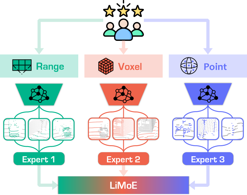
Figure 1: Illustration of the proposed mixture of LiDAR representation learning (LiMoE) design. We observe unique patterns of each LiDAR representation (range, voxel, and point) in image-to-LiDAR data pretraining. Our framework aims to integrate distinct attributes from different LiDAR representations into a unified feature space, enabling enhanced 3D scene understanding.

Recently, data representation learning has emerged as a promising solution to this challenge. By leveraging large-scale, easily accessible datasets, representation learning enables the extraction of meaningful data attributes without heavy reliance on manual annotations [3, 86]. One line of this research [80, 90] augments point clouds into different views and employs contrastive learning across these views for feature consistency. The other line [49, 66, 47, 84] transfers knowledge from the image [27, 19] to LiDAR space [15], facilitating cross-modal learning for large-scale LiDAR scene understanding. However, these methods rely solely on sparse voxels [15], failing to fully explore the complementary information existing in the LiDAR scene.

LiDAR data can be converted into various representations, i.e., range view, sparse voxels, and raw points, each offering unique advantages. Range images provide a compact 2D representation that excels at capturing dynamic elements and medium-range objects [54, 83, 38]. Raw points preserve fine geometric details, enabling precise modeling of intricate structures [32, 85]. Sparse voxels efficiently represent static objects and sparse regions, making them ideal for large-scale environments [94, 15, 30]. Harnessing the complementary strengths of these representations holds the key to robust and comprehensive LiDAR-based perception.

In this work, we present LiMoE, a novel framework that synergistically integrates three LiDAR representations into a unified representation for feature learning. The framework operates in three stages: Image-to-LiDAR pretraining, where knowledge from pretrained image backbone is transferred to LiDAR points for each representation [66, 84], initializing diverse representation-specific features; Contrastive mixture learning (CML), which fuses pretrained features across representations into a unified representation, leveraging their complementary strengths; and Semantic mixture supervision (SMS), which enhances downstream performance by combining multiple semantic logits.

We observe that pretrained models with different LiDAR representations capture distinct data attributes (see Fig. 1). Range images primarily focus on middle laser beams and distances, sparse voxels emphasize upper beams and longer distances, while points capture lower beams and near distances. To effectively integrate these complementary attributes into a unified representation, CML employs a Mixture of Experts (MoE) layer that dynamically activates the relevant data attributes during pretraining. By distilling the combined features into a single representation feature, CML encourages the pretrained network to comprise comprehensive attributes derived from various representations.

In the downstream stage, we observe that different representation models capture distinct object attributes. Range images primarily focus on dynamic objects, sparse voxels emphasize static background structures, while points preserve fine-grained details. To further improve downstream performance, we extend the MoE layer into SMS, which dynamically activates relevant semantic features from various representations. With the supervision of semantic labels, SMS establishes a robust and scalable framework that enhances 3D scene understanding by leveraging complementary semantic features from each LiDAR representation.

To summarize, this work makes contributions as follows:

• We propose LiMoE, a novel framework that integrates multiple LiDAR representations dynamically through the MoE paradigm. To our knowledge, this is the first work to explore MoE for LiDAR representation learning.

• We introduce a three-stage pipeline for enhanced LiDAR scene understanding, comprising knowledge transfer from images to LiDAR, the mixture of data attributes for single-representation pretraining, and integration of semantic attributes for downstream tasks, which offers a robust solution for LiDAR representation learning.

• Extensive experiments verify the effectiveness of our approach, achieving large gains over the state-of-the-art method on $11$ datasets, paving the way for developing scalable, robust, and generalizable automotive systems.

2 Related Work

LiDAR Data Representations. LiDAR point clouds, being irregular and unstructured, pose significant challenges for scene understanding [24, 51, 31]. Recent approaches have sought to address this by transforming point clouds into structured representations. Point-based methods [32, 69, 85] process point clouds directly, preserving their full structure and enabling the capture of fine-grained details. Range view-based methods [54, 38, 83, 81, 18] and bird’s eye view-based methods [89, 92, 11] convert point clouds into 2D representations, leveraging image-processing techniques for efficient identification of dynamic or significant objects. Voxel-based methods [15, 94, 30] discretize point clouds into regular voxel grids and use sparse convolutions [73, 74, 17] to efficiently process sparse regions within the data, making them suitable for large-scale environments.

Multi-Representation LiDAR Segmentation. To capture comprehensive information from various LiDAR representations, recent works have combined multiple representations to explore their complementary strengths [48, 61]. AMVNet [45] and RPVNet [82] employ late-fusion strategies, where features from each representation are processed independently and fused at the final stage. GFNet [62] introduces a more advanced fusion method by combining features from multiple views at different stages. UniSeg [46] uses hierarchical fusion to integrate low-level features with high-level semantic information. In contrast, our approach leverages the Mixture of Experts (MoE) framework, which dynamically activates the most relevant features from multiple representations based on task context.

Image-to-LiDAR Data Pretraining. Inspired by the success of self-supervised learning in the image domain [12, 28, 29], recent work has explored 3D data representation learning [80, 90, 6, 67], which are limited to single-modality learning for small-scale scenes. The SLidR framework [66] introduced multi-modal self-supervised learning by transferring 2D image knowledge to 3D LiDAR models using contrastive learning. Subsequent works expanded this framework with class balancing [52], hybrid-view distillation [88], VFM-assisted superpixels [47], spatiotemporal cues [84], etc. Our work builds upon this by extending image-to-LiDAR pretraining to multiple LiDAR representations, capturing comprehensive LiDAR attributes.

Mixture of Experts. The Mixture of Experts (MoE) framework consists of multiple sub-models that collectively enhance the model’s capacity [53, 8, 21]. MoE dynamically selects a subset of experts to activate based on input, which increases scalability and flexibility for handling diverse tasks. This approach has been widely successful in Large Language Models (LLMs) [20, 22, 44, 91, 93]. Recently, MoE has been applied to vision tasks, including image classification [14, 68, 64], object detection [76, 13, 33], and segmentation [59, 35]. However, MoE remains underexplored in 3D perception. In this work, we extend MoE to 3D data representation, enabling dynamic fusion of multiple LiDAR representations for improved scene understanding.

3 Methodology

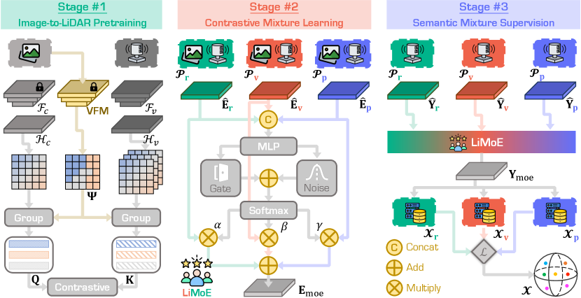
Figure 2: Overview of the LiMoE framework. Our design consists of three stages: (#1) The image-to-LiDAR pretraining transfers knowledge from images to various LiDAR representations (cf. Sec. 3.2); (#2) The contrastive mixture learning (CML) integrates the MoE framework to mix data attributes into a unified representation for pretraining (cf. Sec. 3.3); and (#3) The semantic mixture supervision (SMS) fuses semantic logits from multiple representations to further enhance performance across different downstream tasks (cf. Sec. 3.4).

This work addresses LiDAR-based perception by leveraging multiple data representations to capture complementary information and enhance 3D scene understanding. We first describe the three common LiDAR representations and analyze their strengths (Sec. 3.1). Then, we detail the components of the LiMoE framework, as illustrated in Fig. 2. This comprises three stages: cross-sensor knowledge transfer from images to LiDAR data (Sec. 3.2); mixture of LiDAR data attributes for pretraining (Sec. 3.3); mixture of semantic attributes, supervised by human-annotated labels, for downstream segmentation tasks (Sec. 3.4).

3.1 LiDAR Representation

Let $\mathcal{P}=\{\mathbf{p}_{i}\mid i=1,\ldots,N\}$ denote a LiDAR point cloud consisting of $N$ points, where each point $\mathbf{p}_{i}\in\mathbb{R}^{3+L}$ includes 3D coordinates $(x_{i},y_{i},z_{i})$ and $L$-dimensional features (e.g., intensity, elongation). To harness the unstructured and irregular points, various methods convert point clouds into intermediate representations, including range images $\mathcal{P}_{{\color[rgb]{0,0.70703125,0.546875}\mathbf{r}}}$, sparse voxels $\mathcal{P}_{{\color[rgb]{0.9375,0.38671875,0.29296875}\mathbf{v}}}$, and raw points $\mathcal{P}_{{\color[rgb]{0.38671875,0.44140625,0.98046875}\mathbf{p}}}$.

Range View. The range image methods project the point cloud $\mathcal{P}$ onto 2D grids in spherical coordinates. Each point $\mathbf{p}_{i}$ is mapped to a 2D grid $(u_{i}^{r},v_{i}^{r})$ in the range image as:

$$\binom{u_{i}^{r}}{v_{i}^{r}}=\binom{\frac{1}{2}\left[1-\arctan(y_{i},x_{i})\pi^{-1}\right]W_{r}}{\left[1-(\arcsin(z_{i}d_{i}^{-1})+\phi_{\text{down}})\phi^{-1}H_{r}\right]}~,$$ (1)

where $d_{i}$ represents the depth of the point; $\phi$ denotes the vertical field-of-view of the sensor; $\phi_{\text{down}}$ is the inclination angles in the downward directions; $H_{r}$ and $W_{r}$ are the height and width of the range image. This projection results in a range image $\mathcal{P}_{{\color[rgb]{0,0.70703125,0.546875}\mathbf{r}}}\in\mathbb{R}^{H_{r}\times W_{r}\times(3+L)}$, allowing for efficient processing with image-based techniques. Range images offer a compact 2D representation of the 3D scene, capturing both geometric and intensity-based features [54, 38]. They are particularly effective in tackling dynamic or significant objects in the scene [83, 43].

Sparse Voxels. The voxel-based methods discretize the point cloud $\mathcal{P}$ into regular voxel grids $\mathcal{P}_{{\color[rgb]{0.9375,0.38671875,0.29296875}\mathbf{v}}}$, where each voxel represents a small region of 3D space. For each point $\mathbf{p}_{i}$, its position is mapped to the corresponding voxel grid index as $[v_{i}^{x},v_{i}^{y},v_{i}^{z}]=[\lfloor x_{i}/s_{x}\rfloor,\lfloor y_{i}/s_{y}\rfloor,\lfloor z_{i}/s_{z}\rfloor]$, where $(s_{x},s_{y},s_{z})$ are the voxel sizes along the $x$, $y$ and $z$ dimensions. This discretization results in sparse voxel grids $\mathcal{P}_{{\color[rgb]{0.9375,0.38671875,0.29296875}\mathbf{v}}}\in\mathbb{R}^{M\times C}$, where $M<N$ is the number of non-empty voxels. To effectively process sparse voxels, sparse convolutions [15, 73, 74, 17] are employed, significantly reducing the computational complexity compared to regular voxel grids. Sparse voxels are particularly well-suited for representing large, sparsely populated areas, but can lose detail in dense regions due to quantization effects [15, 94].

Raw Points. The point-based methods process the point cloud (i.e., $\mathcal{P}_{{\color[rgb]{0.38671875,0.44140625,0.98046875}\mathbf{p}}}=\mathcal{P}$) without converting to other representations. These methods typically involve three key steps: 1) Sampling a set of central points (centroids) from the point cloud; 2) Neighbor search, where points in the vicinity of each centroid are identified based on spatial proximity; 3) Feature aggregation, where MLPs are used to combine the features of neighboring points and propagate them to the centroids. While raw points preserve the fine-grained structure of the scene, they are computationally expensive due to the need for point-wise operations [32, 85].

3.2 Image-to-LiDAR Pretraining

Image-to-LiDAR pretraining aims to transfer knowledge from images to LiDAR data, facilitating the learning of effective 3D representations even in the absence of extensive LiDAR labels. Previous works [66, 52, 47, 84] have largely focused on sparse voxel representations for this task, as they offer efficient processing for large-scale LiDAR data.

Given a set of $V$ synchronized images $\mathcal{I}=\{\mathbf{I}_{i}\mid i=1,\ldots,V\}$ and their corresponding LiDAR point clouds $\mathcal{P}$, where each image $\mathbf{I}\in\mathbb{R}^{H\times W\times 3}$ has a spatial resolution with height $H$ and width $W$. Each LiDAR point $\mathbf{p}_{i}$ can be projected onto the corresponding image plane $(u_{i},v_{i})$ as:

$$[u_{i},v_{i}]^{\text{T}}=(1/{z_{i}})\times\Gamma_{K}\times\Gamma_{l\to c}\times[x_{i},y_{i},z_{i}]^{\text{T}}~,$$ (2)

where $\Gamma_{l\to c}$ is the transformation matrix from the LiDAR to the camera coordinate system, and $\Gamma_{K}$ is the camera intrinsic matrix. This pretraining process involves two key steps, as shown on the left side (Phase #1) of Fig. 2.

Superpixel & Superpoint Generation. To establish correlations between images and the point cloud, prior works use the unsupervised SLIC algorithm [1] or vision foundation models (VFMs) [36, 96, 95, 87] to generate a set of $S$ superpixels for each image, denoted as $\mathbf{\Psi}=\{\mathbf{\psi}_{i}\mid i=1,\ldots,S\}$. The corresponding superpoint set $\mathbf{\Omega}=\{\mathbf{\omega}_{i}\mid i=1,\ldots,S\}$ is then derived by projecting these superpixels onto the point cloud using the transformation in Eq. 2.

Contrastive Objective. To transfer the knowledge from images to LiDAR, both image and sparse voxel data are passed through their respective backbones: the 2D pretrained backbone $\mathcal{F}_{c}$ for images and the 3D voxel backbone $\mathcal{F}_{{\color[rgb]{0.9375,0.38671875,0.29296875}\mathbf{v}}}$ for sparse voxels. This generates the respective image and voxel features. These features are then processed by linear projection heads $\mathcal{H}_{c}$ and $\mathcal{H}_{{\color[rgb]{0.9375,0.38671875,0.29296875}\mathbf{v}}}$, which align the feature spaces and produce $D$-dimensional feature embeddings. The image and voxel features are then grouped based on superpixels $\mathbf{\Psi}$ and superpoints $\mathbf{\Omega}$, resulting in superpixel embeddings $\mathbf{Q}\in\mathbb{R}^{S\times D}$ and superpoint embeddings $\mathbf{K}\in\mathbb{R}^{S\times D}$. Finally, a contrastive loss is applied to ensure that each superpoint embedding is closely correlated with its corresponding superpixel embedding:

$$\mathcal{L}_{\text{con}}=\frac{1}{S}\sum_{i=1}^{S}\log\frac{e^{\langle\mathbf{k}_{i},\mathbf{q}_{i}\rangle/\tau}}{\sum_{j\neq i}e^{\langle\mathbf{k}_{i},\mathbf{q}_{j}\rangle/\tau}}~,$$ (3)

where $\langle\cdot,\cdot\rangle$ denotes the dot product between the superpixel and superpoint embeddings, and $\tau>0$ is a temperature.

However, sparse voxel-based pretraining is limited in its ability to fully exploit the detailed geometry and appearance characteristics of 3D scenes. In fact, LiDAR point clouds can be represented in various forms, each emphasizing different attributes, such as laser beams, distance, and static/dynamic objects, within the scene [82]. To this end, we propose a novel pretraining paradigm that integrates multiple representations of LiDAR point clouds. This approach enables a more comprehensive understanding of the scenes by capturing both geometric and detailed information across diverse representations, ultimately constructing a richer, more detailed representation of 3D environments.

3.3 CML: Contrastive Mixture Learning

We extend the image-to-LiDAR pretraining method by independently training three separate 3D networks for each representation: range images, sparse voxels, and raw points. These networks serve as the foundation for our CML approach. As shown in the middle of Fig. 2, each network processes the point cloud in its respective representation form:

$$\mathbf{E}_{{\color[rgb]{0,0.70703125,0.546875}\mathbf{r}}} =\mathcal{H}_{{\color[rgb]{0,0.70703125,0.546875}\mathbf{r}}}(\mathcal{F}_{{\color[rgb]{0,0.70703125,0.546875}\mathbf{r}}}(\mathcal{P}_{{\color[rgb]{0,0.70703125,0.546875}\mathbf{r}}}))\in\mathbb{R}^{H_{r}\times W_{r}\times D}~,$$

$$\mathbf{E}_{{\color[rgb]{0.9375,0.38671875,0.29296875}\mathbf{v}}} =\mathcal{H}_{{\color[rgb]{0.9375,0.38671875,0.29296875}\mathbf{v}}}(\mathcal{F}_{{\color[rgb]{0.9375,0.38671875,0.29296875}\mathbf{v}}}(\mathcal{P}_{{\color[rgb]{0.9375,0.38671875,0.29296875}\mathbf{v}}}))\in\mathbb{R}^{M\times D}~,$$ (4)

$$\mathbf{E}_{{\color[rgb]{0.38671875,0.44140625,0.98046875}\mathbf{p}}} =\mathcal{H}_{{\color[rgb]{0.38671875,0.44140625,0.98046875}\mathbf{p}}}(\mathcal{F}_{{\color[rgb]{0.38671875,0.44140625,0.98046875}\mathbf{p}}}(\mathcal{P}_{{\color[rgb]{0.38671875,0.44140625,0.98046875}\mathbf{p}}}))\in\mathbb{R}^{N\times D}~.$$

Following the success of the Mixture of Experts (MoE) approach [91, 44], we introduce an MoE layer that dynamically selects and combines relevant features from different representations for each point.

(a) Expert Activation Paths (Beam Number)

(b) Expert Activation Paths (Distances to Ego)

Figure 3: Visual interpretations of the expert activation paths in CML. The experts are #1 range view, #2 voxel, and #3 point, respectively.

Feature Alignment. The features generated from each representation, as in Sec. 3.3, vary significantly due to the different representation attributes. To align these features, we project the range image and sparse voxel features into the point cloud space. This results in aligned feature sets $\widehat{\mathbf{E}}_{{\color[rgb]{0,0.70703125,0.546875}\mathbf{r}}}$, $\widehat{\mathbf{E}}_{{\color[rgb]{0.9375,0.38671875,0.29296875}\mathbf{v}}}$, and $\widehat{\mathbf{E}}_{{\color[rgb]{0.38671875,0.44140625,0.98046875}\mathbf{p}}}$, all with the form $\mathbb{R}^{N\times D}$, ensuring consistent feature space across these three representations.

MoE Layer. This layer takes $\widehat{\mathbf{E}}_{{\color[rgb]{0,0.70703125,0.546875}\mathbf{r}}}$, $\widehat{\mathbf{E}}_{{\color[rgb]{0.9375,0.38671875,0.29296875}\mathbf{v}}}$, and $\widehat{\mathbf{E}}_{{\color[rgb]{0.38671875,0.44140625,0.98046875}\mathbf{p}}}$ as the input. To combine the features from these three representations, we first concatenate them and then apply an MLP layer to reduce the channel dimension. The MoE layer consists of two key components: a gate module, which dynamically selects the activated representation for each point, and a noise module, which introduces perturbations to prevent overfitting. This process can be formulated as follows:

$$\mathbf{G} =\mathbf{E}\cdot\mathbf{Z}_{g}+\chi\cdot\sigma(\mathbf{E}\cdot\mathbf{Z}_{n})~,$$ (5)

$$\mathbf{E} =\text{MLP}([\widehat{\mathbf{E}}_{{\color[rgb]{0,0.70703125,0.546875}\mathbf{r}}},\widehat{\mathbf{E}}_{{\color[rgb]{0.9375,0.38671875,0.29296875}\mathbf{v}}},\widehat{\mathbf{E}}_{{\color[rgb]{0.38671875,0.44140625,0.98046875}\mathbf{p}}}])~.$$ (6)

Here, $\mathbf{Z}_{g}\in\mathbb{R}^{D\times 3}$ and $\mathbf{Z}_{n}\in\mathbb{R}^{D\times 3}$ are trainable weights for the gate and noise modules, respectively. The variable $\chi$ represents a random noise distribution, which is applied in the noise module to introduce variability into the feature selection process. The function $\sigma$ denotes the Softplus activation, ensuring that the perturbations remain positive and smooth. The operation $[\cdot,\cdot]$ denotes feature concatenation. A softmax function is then applied to the gate values $\mathbf{G}$, yielding selection scores $\widehat{\mathbf{G}}\in\mathbb{R}^{N\times 3}$. These scores are then split into $\alpha$, $\beta$, and $\gamma$ for each representation, respectively, indicating the importance of each representation for each point. The final output features are obtained by weighting and summing the features from each representation: $\mathbf{E}_{\text{moe}}=\alpha\widehat{\mathbf{E}}_{{\color[rgb]{0,0.70703125,0.546875}\mathbf{r}}}+\beta\widehat{\mathbf{E}}_{{\color[rgb]{0.9375,0.38671875,0.29296875}\mathbf{v}}}+\gamma\widehat{\mathbf{E}}_{{\color[rgb]{0.38671875,0.44140625,0.98046875}\mathbf{p}}}$. These features capture the dynamic contributions of each representation, enabling the model to adaptively prioritize the most relevant features for each point in the LiDAR point cloud. This selective feature fusion enables the network to leverage the strengths of each representation dependent on the context, thereby improving its ability to capture detailed scene attributes.

Training Objective. In this stage, the goal is to distill the MoE features from multiple representations into a single LiDAR representation (range, voxel, or point). To accomplish this, we use a 3D student network to extract corresponding student features $\mathbf{E}_{l}^{s}=\mathcal{H}_{l}^{s}(\mathcal{F}_{l}^{s}(\mathcal{P}_{l}))$ ($l\in\{{\color[rgb]{0,0.70703125,0.546875}\mathbf{r}},{\color[rgb]{0.9375,0.38671875,0.29296875}\mathbf{v}},{\color[rgb]{0.38671875,0.44140625,0.98046875}\mathbf{p}}\}$). Then, the MoE features and student features are grouped based on superpoints to generate the superpoint embeddings $\mathbf{K}^{\text{moe}}$ and $\mathbf{K}^{l}$. A contrastive loss is then applied between them as:

$$\mathcal{L}_{\text{CML}}=\frac{1}{S}\sum_{i=1}^{S}\log\frac{e^{\langle\mathbf{k}_{i}^{l},\mathbf{k}_{i}^{\text{moe}}\rangle/\tau}}{\sum_{j\neq i}e^{\langle\mathbf{k}_{i}^{l},\mathbf{k}_{j}^{\text{moe}}\rangle/\tau}}~.$$ (7)

The contrastive loss encourages the student features to align with the MoE features, allowing the single 3D student network to effectively capture informative structures from all the different representations. As depicted in Fig. 3, CML encourages the MoE framework to focus on data attributes from laser beams and distances.

3.4 SMS: Semantic Mixture Supervision

To further improve downstream semantic segmentation performance, we extend the MoE layer into the downstream tasks, as shown in the right side of Fig. 2. This integration enables the model to dynamically select and prioritize the most relevant object attributes from each representation, tailoring feature fusion to the specific context of the task. Building upon the pretrained representations in Sec. 3.3, each backbone independently processes the point cloud to generate semantic logits for each representation:

$$\mathbf{Y}_{{\color[rgb]{0,0.70703125,0.546875}\mathbf{r}}} =\widetilde{\mathcal{H}}_{{\color[rgb]{0,0.70703125,0.546875}\mathbf{r}}}^{s}(\mathcal{F}_{{\color[rgb]{0,0.70703125,0.546875}\mathbf{r}}}^{s}(\mathcal{P}_{{\color[rgb]{0,0.70703125,0.546875}\mathbf{r}}}))\in\mathbb{R}^{H_{r}\times W_{r}\times C}~,$$

$$\mathbf{Y}_{{\color[rgb]{0.9375,0.38671875,0.29296875}\mathbf{v}}} =\widetilde{\mathcal{H}}_{{\color[rgb]{0.9375,0.38671875,0.29296875}\mathbf{v}}}^{s}(\mathcal{F}_{{\color[rgb]{0.9375,0.38671875,0.29296875}\mathbf{v}}}^{s}(\mathcal{P}_{{\color[rgb]{0.9375,0.38671875,0.29296875}\mathbf{v}}}))\in\mathbb{R}^{M\times C}~,$$ (8)

$$\mathbf{Y}_{{\color[rgb]{0.38671875,0.44140625,0.98046875}\mathbf{p}}} =\widetilde{\mathcal{H}}_{{\color[rgb]{0.38671875,0.44140625,0.98046875}\mathbf{p}}}^{s}(\mathcal{F}_{{\color[rgb]{0.38671875,0.44140625,0.98046875}\mathbf{p}}}^{s}(\mathcal{P}_{{\color[rgb]{0.38671875,0.44140625,0.98046875}\mathbf{p}}}))\in\mathbb{R}^{N\times C}~,$$

where $C$ is the number of semantic classes. $\widetilde{\mathcal{H}}_{{\color[rgb]{0,0.70703125,0.546875}\mathbf{r}}}^{s}$, $\widetilde{\mathcal{H}}_{{\color[rgb]{0.9375,0.38671875,0.29296875}\mathbf{v}}}^{s}$, and $\widetilde{\mathcal{H}}_{{\color[rgb]{0.38671875,0.44140625,0.98046875}\mathbf{p}}}^{s}$ are linear heads that project backbone features into semantic logits for each representation. To align logits across representations, we project them into the point cloud space, yielding $\widehat{\mathbf{Y}}_{{\color[rgb]{0,0.70703125,0.546875}\mathbf{r}}}$, $\widehat{\mathbf{Y}}_{{\color[rgb]{0.9375,0.38671875,0.29296875}\mathbf{v}}}$, and $\widehat{\mathbf{Y}}_{{\color[rgb]{0.38671875,0.44140625,0.98046875}\mathbf{p}}}$, each with a form of $\mathbb{R}^{N\times C}$.

The MoE layer consists of a gating module that dynamically selects the activated representations for each point, and a noise module that introduces perturbations to the features during training to mitigate overfitting. Different from Eq. 5, the noise gate is only active during training. The whole process can be formulated as:

$$\mathbf{G}_{d}=\mathbf{Y}\cdot\mathbf{Z}_{g}+\zeta\cdot\chi\cdot\sigma(\mathbf{Y}\cdot\mathbf{Z}_{n})~,$$ (9)

where $\zeta=1$ for training and $\zeta=0$ for inference, and $\mathbf{Y}=\text{MLP}([\widehat{\mathbf{Y}}_{{\color[rgb]{0,0.70703125,0.546875}\mathbf{r}}},\widehat{\mathbf{Y}}_{{\color[rgb]{0.9375,0.38671875,0.29296875}\mathbf{v}}},\widehat{\mathbf{Y}}_{{\color[rgb]{0.38671875,0.44140625,0.98046875}\mathbf{p}}}])$. After applying the softmax function to the gate value $\mathbf{G}_{d}$, we obtain the coefficients $\alpha_{d}$, $\beta_{d}$, and $\gamma_{d}$, which indicate the relative importance of each representation for every point. The final semantic logits are obtained by a weighted sum of the logits from each representation: $\mathbf{Y}_{\text{moe}}=\alpha_{d}\widehat{\mathbf{Y}}_{{\color[rgb]{0,0.70703125,0.546875}\mathbf{r}}}+\beta_{d}\widehat{\mathbf{Y}}_{{\color[rgb]{0.9375,0.38671875,0.29296875}\mathbf{v}}}+\gamma_{d}\widehat{\mathbf{Y}}_{{\color[rgb]{0.38671875,0.44140625,0.98046875}\mathbf{p}}}$.

Table 1: Comparisons of state-of-the-art LiDAR pretraining methods pretrained on nuScenes [7] and fine-tuned on nuScenes [23], SemanticKITTI [2], and Waymo Open [71] datasets, respectively, with specified data portions. LP denotes linear probing with frozen backbones. All scores are given in percentage (%). The best and 2nd best scores under each group are highlighted in bold and underline.

Method	Venue	Backbone	Backbone	Expert	nuScenes						KITTI	Waymo
		(2D)	(3D)		LP	1%	5%	10%	25%	Full	1%	1%
Random	-	-	-	-	$8.10$	$30.30$	$47.84$	$56.15$	$65.48$	$74.66$	$39.50$	$39.41$
SLidR [66]	CVPR’22	ResNet-50 [27]	MinkUNet-34 [15]	Single $\circ$	$38.80$	$38.30$	$52.49$	$59.84$	$66.91$	$74.79$	$44.60$	$47.12$
TriCC [58]	CVPR’23			Single $\circ$	$38.00$	$41.20$	$54.10$	$60.40$	$67.60$	$75.60$	$45.90$	$-$
Seal [47]	NeurIPS’23			Single $\circ$	$44.95$	$45.84$	$55.64$	$62.97$	$68.41$	$75.60$	$46.63$	$\mathbf{49.34}$
CSC [9]	CVPR’24			Single $\circ$	$\mathbf{46.00}$	$\mathbf{47.00}$	$\mathbf{57.00}$	$\mathbf{63.30}$	$68.60$	$75.70$	$47.20$	$-$
HVDistill [88]	IJCV’24			Single $\circ$	$39.50$	$42.70$	$56.60$	$62.90$	$\mathbf{69.30}$	$\mathbf{76.60}$	$\mathbf{49.70}$	$-$
SLidR [66]	CVPR’22	ViT-S [56]	MinkUNet-34 [15]	Single $\circ$	$44.70$	$41.16$	$53.65$	$61.47$	$66.71$	$74.20$	$44.67$	$47.57$
+ LiMoE	Ours			Multi $\bullet$	$45.80$	$46.82$	$57.54$	$63.85$	$68.61$	$75.64$	$46.81$	$48.81$
Seal [47]	NeurIPS’23			Single $\circ$	$45.16$	$44.27$	$55.13$	$62.46$	$67.64$	$75.58$	$46.51$	$48.67$
SuperFlow [84]	ECCV’24			Single $\circ$	$46.44$	$47.81$	$59.44$	$64.47$	$69.20$	$76.54$	$47.97$	$49.94$
+ LiMoE	Ours			Multi $\bullet$	$\mathbf{48.20}$	$\mathbf{49.60}$	$\mathbf{60.54}$	$\mathbf{65.65}$	$\mathbf{71.39}$	$\mathbf{77.27}$	$\mathbf{49.53}$	$\mathbf{51.42}$
SLidR [66]	CVPR’22	ViT-B [56]	MinkUNet-34 [15]	Single $\circ$	$45.35$	$41.64$	$55.83$	$62.68$	$67.61$	$74.98$	$45.50$	$48.32$
+ LiMoE	Ours			Multi $\bullet$	$46.56$	$46.89$	$58.09$	$63.87$	$69.02$	$75.87$	$47.96$	$49.50$
Seal [47]	NeurIPS’23			Single $\circ$	$46.59$	$45.98$	$57.15$	$62.79$	$68.18$	$75.41$	$47.24$	$48.91$
SuperFlow [84]	ECCV’24			Single $\circ$	$47.66$	$48.09$	$59.66$	$64.52$	$69.79$	$76.57$	$48.40$	$50.20$
+ LiMoE	Ours			Multi $\bullet$	$\mathbf{49.07}$	$\mathbf{50.23}$	$\mathbf{61.51}$	$\mathbf{66.17}$	$\mathbf{71.56}$	$\mathbf{77.81}$	$\mathbf{50.30}$	$\mathbf{51.77}$
SLidR [66]	CVPR’22	ViT-L [56]	MinkUNet-34 [15]	Single $\circ$	$45.70$	$42.77$	$57.45$	$63.20$	$68.13$	$75.51$	$47.01$	$48.60$
+ LiMoE	Ours			Multi $\bullet$	$47.43$	$46.92$	$58.41$	$64.54$	$69.69$	$76.32$	$48.25$	$50.23$
Seal [47]	NeurIPS’23			Single $\circ$	$46.81$	$46.27$	$58.14$	$63.27$	$68.67$	$75.66$	$47.55$	$50.02$
SuperFlow [84]	ECCV’24			Single $\circ$	$48.01$	$49.95$	$60.72$	$65.09$	$70.01$	$77.19$	$49.07$	$50.67$
+ LiMoE	Ours			Multi $\bullet$	$\mathbf{49.35}$	$\mathbf{51.41}$	$\mathbf{62.07}$	$\mathbf{66.64}$	$\mathbf{71.59}$	$\mathbf{77.85}$	$\mathbf{50.69}$	$\mathbf{51.93}$

Table 2: Domain generalization study of different LiDAR pretraining methods pretrained on the nuScenes [7] dataset and fine-tuned on a collection of seven different LiDAR semantic segmentation datasets [75, 34, 57, 79, 77, 37, 65], respectively, with specific data portions. All scores are given in percentage (%). The best and 2nd best scores from each metric are highlighted in bold and underline.

Method	Venue	ScriKITTI		Rellis-3D		SemPOSS		SemSTF		SynLiDAR		DAPS-3D		Synth4D
		1%	10%	1%	10%	Half	Full	Half	Full	1%	10%	Half	Full	1%	10%
Random	-	$23.81$	$47.60$	$38.46$	$53.60$	$46.26$	$54.12$	$48.03$	$48.15$	$19.89$	$44.74$	$74.32$	$79.38$	$20.22$	$66.87$
PPKT [49]	arXiv’21	$36.50$	$51.67$	$49.71$	$54.33$	$50.18$	$56.00$	$50.92$	$54.69$	$37.57$	$46.48$	$78.90$	$84.00$	$61.10$	$62.41$
SLidR [66]	CVPR’22	$39.60$	$50.45$	$49.75$	$54.57$	$51.56$	$55.36$	$52.01$	$54.35$	$42.05$	$47.84$	$81.00$	$85.40$	$63.10$	$62.67$
+ LiMoE	Ours	$41.48$	$53.41$	$51.28$	$55.21$	$53.14$	$56.42$	$53.16$	$55.51$	$43.72$	$49.57$	$81.70$	$85.76$	$64.69$	$66.79$
Seal [47]	NeurIPS’23	$40.64$	$52.77$	$51.09$	$55.03$	$53.26$	$56.89$	$53.46$	$55.36$	$43.58$	$49.26$	$81.88$	$85.90$	$64.50$	$66.96$
SuperFlow [84]	ECCV’24	$42.70$	$54.00$	$52.83$	$55.71$	$54.41$	$57.33$	$54.72$	$56.57$	$44.85$	$51.38$	$82.43$	$86.21$	$65.31$	$69.43$
+ LiMoE	Ours	$\mathbf{43.95}$	$\mathbf{55.96}$	$\mathbf{53.74}$	$\mathbf{56.67}$	$\mathbf{55.42}$	$\mathbf{57.83}$	$\mathbf{55.60}$	$\mathbf{57.31}$	$\mathbf{45.79}$	$\mathbf{52.27}$	$\mathbf{83.24}$	$\mathbf{86.68}$	$\mathbf{66.54}$	$\mathbf{71.07}$

Training Objective. Let $\mathcal{X}\in\mathbb{R}^{N}$ denote the semantic labels for the point cloud $\mathcal{P}$. For each representation, these labels can be projected as follows: $\mathcal{X}_{{\color[rgb]{0,0.70703125,0.546875}\mathbf{r}}}\in\mathbb{R}^{H_{r}\times W_{r}}$ for the range image, $\mathcal{X}_{{\color[rgb]{0.9375,0.38671875,0.29296875}\mathbf{v}}}\in\mathbb{R}^{M}$ for the sparse voxels, and $\mathcal{X}_{{\color[rgb]{0.38671875,0.44140625,0.98046875}\mathbf{p}}}\in\mathbb{R}^{N}$ for raw points. Each representation is fine-tuned independently with a supervised loss that aligns the predicted logits with the corresponding projected semantic labels. In addition, we apply an MoE-based supervised loss at the output to further refine the model by selecting the most relevant features from each representation. The overall loss is:

$$\mathcal{L}_{\text{SMS}}=\mathcal{L}_{\text{d}}(\mathcal{X},\mathbf{Y}_{\text{moe}})~~+\sum_{l\in\{{\color[rgb]{0,0.70703125,0.546875}\mathbf{r}},{\color[rgb]{0.9375,0.38671875,0.29296875}\mathbf{v}},{\color[rgb]{0.38671875,0.44140625,0.98046875}\mathbf{p}}\}}\mathcal{L}_{l}(\mathcal{X}_{l},\mathbf{Y}_{l})~,$$ (10)

where each $\mathcal{L}_{l}$ (for $l\in\{d,{\color[rgb]{0,0.70703125,0.546875}\mathbf{r}},{\color[rgb]{0.9375,0.38671875,0.29296875}\mathbf{v}},{\color[rgb]{0.38671875,0.44140625,0.98046875}\mathbf{p}}\}$) is a weighted combination of Cross-Entropy, Lovasz-Softmax [4], and Boundary loss [63], contributing to a comprehensive optimization of the segmentation performance across all representations.

4 Experiments

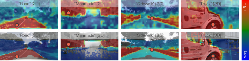
Figure 4: Cosine similarity between learned features of a query point (denoted as the red dot) and: (1) the features of the image of the same scene (the first row); and (2) the features of the LiDAR points projected onto the image (the second row). Best viewed in colors.

Table 3: Out-of-distribution robustness assessment of LiDAR pretraining methods under corruptions and sensor failures in the nuScenes-C dataset from the Robo3D benchmark [39]. Full denotes fine-tuning with full labels. LP denotes linear probing with frozen backbones. All mCE, mRR, and mIoU scores are given in percentage (%). The best and 2nd best scores are highlighted in bold and underline.

#	Method	Venue	mCE$\downarrow$	mRR$\uparrow$	Fog$\uparrow$	Rain$\uparrow$	Snow$\uparrow$	Blur$\uparrow$	Beam$\uparrow$	Cross$\uparrow$	Echo$\uparrow$	Sensor$\uparrow$	Average$\uparrow$
Full	Random	-	$112.20$	$72.57$	$62.96$	$70.65$	$55.48$	$51.71$	$62.01$	$31.56$	$59.64$	$39.41$	$54.18$
Full	PPKT [49]	arXiv’21	$105.64$	$75.87$	$64.01$	$72.18$	$59.08$	$57.17$	$63.88$	$36.34$	$60.59$	$39.57$	$56.60$
	SLidR [66]	CVPR’22	$106.08$	$75.99$	$65.41$	$72.31$	$56.01$	$56.07$	$62.87$	$41.94$	$61.16$	$38.90$	$56.83$
	+ LiMoE	Ours	$101.74$	$77.77$	$67.92$	$73.25$	$57.02$	$56.30$	$64.72$	$44.81$	$61.23$	$45.37$	$58.83$
	Seal [47]	NeurIPS’23	$92.63$	$83.08$	$\mathbf{72.66}$	$74.31$	$\mathbf{66.22}$	$\mathbf{66.14}$	$65.96$	$57.44$	$59.87$	$39.85$	$62.81$
	SuperFlow [84]	ECCV’24	$91.67$	$83.17$	$70.32$	$75.77$	$65.41$	$61.05$	$68.09$	$60.02$	$58.36$	$50.41$	$63.68$
	+ LiMoE	Ours	$\mathbf{88.43}$	$\mathbf{83.28}$	$71.10$	$\mathbf{75.92}$	$65.66$	$63.86$	$\mathbf{68.52}$	$\mathbf{60.78}$	$\mathbf{61.91}$	$\mathbf{50.66}$	$\mathbf{64.80}$
LP	PPKT [49]	arXiv’21	$183.44$	$78.15$	$30.65$	$35.42$	$28.12$	$29.21$	$32.82$	$19.52$	$28.01$	$20.71$	$28.06$
	SLidR [66]	CVPR’22	$179.38$	$77.18$	$34.88$	$38.09$	$32.64$	$26.44$	$33.73$	$20.81$	$31.54$	$21.44$	$29.95$
	+ LiMoE	Ours	$163.75$	$75.49$	$37.29$	$43.41$	$36.04$	$38.33$	$40.66$	$22.46$	$37.61$	$25.38$	$35.15$
	Seal [47]	NeurIPS’23	$166.18$	$75.38$	$37.33$	$42.77$	$29.93$	$37.73$	$40.32$	$20.31$	$37.73$	$24.94$	$33.88$
	SuperFlow [84]	ECCV’24	$161.78$	$75.52$	$37.59$	$43.42$	$37.60$	$39.57$	$41.40$	$23.64$	$38.03$	$26.69$	$35.99$
	+ LiMoE	Ours	$\mathbf{155.77}$	$\mathbf{78.23}$	$\mathbf{40.35}$	$\mathbf{45.28}$	$\mathbf{39.14}$	$\mathbf{42.10}$	$\mathbf{44.21}$	$\mathbf{27.33}$	$\mathbf{39.20}$	$\mathbf{29.49}$	$\mathbf{38.39}$

4.1 Configurations

Datasets. Following the practical settings [47, 84], we use the nuScenes [7] for pretraining and evaluate it across 11 LiDAR semantic segmentation datasets, including nuScenes [23], SemanticKITTI [2], Waymo Open [71], ScribbleKITTI [75], RELLIS-3D [34], SemanticPOSS [57], SemanticSTF [79], SynLiDAR [77], DAPS-3D [37], Synth4D [65], and Robo3D [39]. More details are in the Appendix.

Implementation Details. All experiments are conducted using the MMDetection3D [16] codebase. For each LiDAR representation, we select FRNet [83] (range), MinkUNet [15] (voxel), and SPVCNN [72] (point) as the backbones. For image-to-LiDAR pretraining, we adopt the SLidR [66] and SuperFlow [84] paradigms. The learning rate for pretraining is set to 0.01, while the learning rate for the second CML stage is 0.001. In the third stage, we use a separate learning rate scheme: 0.001 for the backbone and 0.01 for other parts. We use the AdamW optimizer [50] and a OneCycle scheduler [70] for all stages. In line with standard protocol, we report the mean Intersection-over-Union (mIoU) for segmentation, as well as mean Corruption Error (mCE) and mean Resilience Rate (mRR) for robustness.

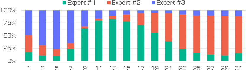
(a) Expert Loadings (Beam Number)

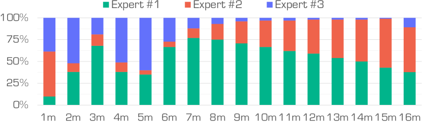
(b) Expert Loadings (Distances to Ego)

Figure 5: Ablation study on distributions of expert loadings in CML. The distributions are based on (a) LiDAR beam numbers and (b) distances. The three experts are #1 range view, #2 voxel, and #3 point, respectively.

4.2 Comparative Study

Comparisons to State of the Arts. In Tab. 1, we compare LiMoE with state-of-the-art pretraining methods using both Linear Probing (LP) and fine-tuning on various portions of the nuScenes [23] dataset. In the LP setting, where the backbone is frozen and only the task-specific head is trained, our approach outperforms single-representation methods [66, 84], achieving mIoU gains from $1.10\%$ to $1.76\%$. In the fine-tuning setting, where both the backbone and task head are updated, we observe even greater improvements, with mIoU gains ranging from $0.66\%$ to $5.66\%$. These results highlight the advantages of combining multiple representations, leading to enhanced performance.

Cross-Dataset Knowledge Transfer. To evaluate the scalability of LiMoE, we conduct a comprehensive study across nine diverse 3D semantic segmentation datasets. Notably, except for the SemanticKITTI [2] and ScribbleKITTI [75] datasets, the remaining seven datasets cannot be effectively converted into range images due to the unknown FoV parameters of their LiDAR sensors. As a result, for these datasets, we combine only voxel and point representations in the SMS stage, since range image representations are not feasible. As shown in Tab. 1 and Tab. 2, our method consistently outperforms single-representation methods across all datasets, demonstrating superior adaptability and robustness for a wide range of 3D segmentation tasks.

Robustness Assessments. The robustness of a 3D perception model against unprecedented conditions is crucial for its development in real-world applications. In Tab. 3, we compare LiMoE with previous pretraining methods using the nuScenes-C dataset from the Robo3D benchmark [39]. The results show that our method excels in handling various types of corruption, demonstrating its robustness and resilience under challenging real-world conditions.

Qualitative Results. Fig. 4 illustrates the similarity between a query point and the pretrained 2D image backbone, as well as other LiDAR points during the CML stage. The visual results confirm that combining multiple representations enhances the semantic features during pretraining, resulting in more effective feature learning.

Table 4: Ablation study on experts in CML. Only sparse voxel representation is employed for the downstream task. All scores are given in percentage (%). The best scores are highlighted in bold.

Pretrain	Experts			nuScenes		KITTI
	Voxel	Point	Range	LP	1%	1%
Random	✓	✗	✗	$8.10$	$30.30$	$39.50$
SLidR [66]	✓	✗	✗	$45.35$	$41.64$	$45.50$
LiMoE	✓	✓	✗	$45.73$	$43.28$	$46.54$
	✓	✗	✓	$45.89$	$43.81$	$46.60$
	✗	✓	✓	$45.56$	$42.56$	$46.21$
	✓	✓	✓	$\mathbf{46.02}$	$\mathbf{44.85}$	$\mathbf{46.92}$

Table 5: Ablation study on experts in SMS. All scores are given in percentage (%). The best scores are highlighted in bold.

Pretrain	Experts			nuScenes		KITTI
	Voxel	Point	Range	LP	1%	1%
	✓	✗	✗	$8.10$	$30.30$	$39.50$
Random	✗	✓	✗	$8.80$	$34.79$	$38.74$
	✗	✗	✓	$11.85$	$29.56$	$39.20$
LiMoE	✓	✗	✗	$46.02$	$44.85$	$46.92$
	✗	✓	✗	$45.97$	$44.79$	$47.06$
	✗	✗	✓	$45.09$	$40.88$	$44.34$
	✓	✓	✗	$46.37$	$45.74$	$47.51$
	✓	✗	✓	$46.28$	$45.70$	$47.35$
	✗	✓	✓	$46.09$	$45.32$	$47.49$
	✓	✓	✓	$\mathbf{46.56}$	$\mathbf{46.89}$	$\mathbf{47.96}$

4.3 Ablation Study

Route Activations. In Fig. 5, we present the distributions of beam numbers and distances loaded by each representation during the CML stage. Range images predominantly capture middle beams and distances, sparse voxels focus on upper beams and longer distances, while points concentrate on lower beams and near distances. This distribution highlights the complementary nature of these representations, which provide a more comprehensive representation of the LiDAR data when combined in the MoE layer. In Fig. 6, we show the distributions of semantic classes loaded by each representation during the SMS stage. Range images are more sensitive to dynamic objects, sparse voxels highlight background objects, and raw points capture more detailed objects with complex structures. These results demonstrate how each representation contributes to the feature fusion.

Scaling LiDAR Representations. In this ablation study, we explore the effect of combining multiple representations in both the CML and SMS stages. First, we test different combinations of representations for pretraining in the CML stage, using a sparse voxel-based network for the downstream task. The results shown in Tab. 4 demonstrate that combining multiple representations consistently outperforms single-representation pretraining. Next, we explore various combinations in the SMS stage, where each representation is pretrained using the CML stage. As presented in Tab. 5, incorporating multiple representations in the SMS stage further boosts performance, validating the advantages of multi-representation fusion in both pretraining and downstream tasks.

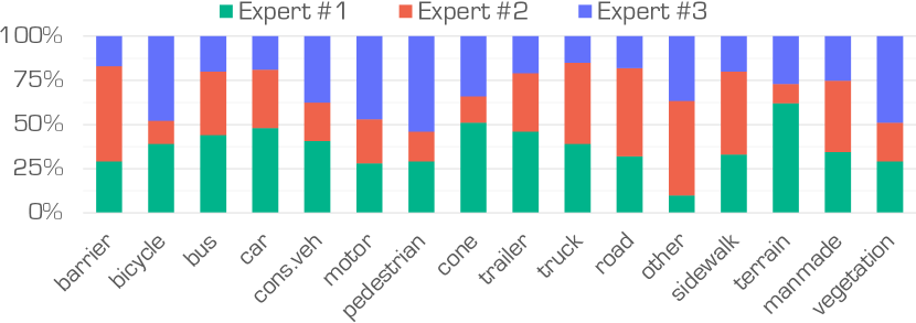
Figure 6: Class-wise expert loadings in SMS. The three experts are #1 range view, #2 voxel, and #3 point, respectively.

Different LiDAR Backbones. In this ablation study, we evaluate the downstream performance of FRNet [83] and SPVCNN [72] across various pretraining strategies. In the LP setting, the networks achieve mIoU scores of $11.85$ and $8.80$ with random initialization. When pretrained with SLidR [66], the mIoU scores improve to $44.01$ and $44.85$, respectively. Pretrained with LiMoE further boosts performance, yielding mIoU scores of $45.09$ and $45.97$. In the fine-tuning setting using $1\%$ annotated data from the nuScenes [23] dataset, the networks achieve mIoU scores of $29.56$ and $34.79$ with random initialization. After pretraining with SLidR [66], the mIoU scores rise to $37.82$ and $41.59$. Notably, pretraining with LiMoE leads to further gains, reaching $40.88$ and $44.79$, respectively. These results underscore the effectiveness and scalability of multi-representation fusion for pretraining.

Downstream Efficiency. Finally, we analyze the impact of LiMoE on downstream efficiency. CML integrates multiple LiDAR representations into a unified network for pretraining, with no impact on downstream efficiency. In contrast, SMS combines multiple representations for downstream tasks, which introduces additional computational costs.

5 Conclusion

In this work, we introduced LiMoE, a novel framework designed to leverage multiple LiDAR representations for enhanced feature learning in LiDAR scenes. By combining range images, sparse voxels, and raw points through a Mixture of Experts framework, our approach captures complementary information from different representations, enabling more robust scene understanding. We proposed a three-stage feature learning process, consisting of Image-to-LiDAR Pretraining, Contrastive Mixture Learning (CML), and Semantic Mixture Supervision (SMS). Extensive experiments demonstrate that our design outperforms existing approaches across multiple benchmarks. We hope this work paves the way for more scalable and robust LiDAR-based perception systems for real-world applications.

Appendix

[appendices] [appendices]l1

6 Additional Implementation Details

In this section, we provide additional details to facilitate the implementation and reproducibility of the methods within the proposed LiMoE framework.

6.1 Datasets

In this work, we conduct extensive experiments across a diverse set of LiDAR semantic segmentation datasets to validate the effectiveness of the proposed LiMoE framework.

• nuScenes [7, 23] is a large-scale, multimodal dataset designed for autonomous driving, featuring six cameras, five radars, one LiDAR, along with IMU and GPS sensors. The dataset comprises $1,000$ driving scenes collected in Boston and Singapore. For the point cloud semantic segmentation task, it provides $1.4$ billion annotated points across $40,000$ point clouds, with each LiDAR point labeled into one of $32$ semantic categories. The point clouds are captured using a Velodyne HDL-32E LiDAR sensor. In this work, a mini-train split is created from the full training set for model pretraining during the Image-to-LiDAR and CML stages, adhering to the SLidR protocol [66]. For the SMS stage, the training set is further split to generate subsets containing $1\%$, $5\%$, $10\%$, $25\%$, and $100\%$ of annotated scans for fine-tuning. More details about this dataset can be found at https://nuscenes.org/nuscenes.

• SemanticKITTI [2] is a large-scale benchmark dataset tailored for semantic scene understanding in autonomous driving. The dataset was collected using a Velodyne HDL-64E LiDAR sensor, capturing diverse real-world scenarios such as urban traffic in city centers, residential neighborhoods, highways, and rural countryside roads around Karlsruhe, Germany. The dataset consists of $22$ densely labeled point cloud sequences derived from the KITTI Odometry benchmark [25], with each point annotated into one of $28$ semantic categories. In this work, the training set is uniformly split to create a subset with $1\%$ of the scans for fine-tuning. More details about this dataset can be found at https://semantic-kitti.org.

• Waymo Open [71] is a large-scale, high-quality, and diverse dataset designed to advance perception in autonomous driving. The dataset features multimodal data collected using five high-resolution cameras and five LiDAR sensors. It includes $1,150$ driving scenes recorded across a variety of suburban and urban areas, captured at different times of the day to ensure diversity in lighting, weather, and traffic conditions. For the LiDAR semantic segmentation task, each point in the dataset is annotated into one of $23$ semantic categories. In this work, the training set is uniformly split to create a subset with $1\%$ of the scans for fine-tuning. More details about this dataset can be found at https://waymo.com/open.

• ScribbleKITTI [75] is a weakly supervised variant of the SemanticKITTI [2] dataset, designed to advance research in semantic scene understanding with minimal annotation effort. Unlike SemanticKITTI, which provides dense, point-wise annotations for every LiDAR point, ScribbleKITTI employs sparse line scribble annotations as a cost-effective alternative. This approach drastically reduces annotation requirements, with the dataset containing approximately $189$ million labeled points – around $8.06\%$ of the fully supervised dataset – resulting in a $90\%$ reduction in annotation time. In this work, the training set is uniformly split to create subsets with $1\%$ and $10\%$ of the scans for fine-tuning. More details about this dataset can be found at https://github.com/ouenal/scribblekitti.

• RELLIS-3D [34] is a multimodal dataset curated for semantic scene understanding in complex off-road environments. It consists of five traversal sequences collected along three unpaved trails on the RELLIS Campus of Texas A&M University. For the LiDAR semantic segmentation task, point-wise annotation was generated by projecting image-based semantic labels onto the point cloud using precise camera-LiDAR calibration. Each LiDAR point is categorized into one of $20$ semantic categories. In this work, the training set is uniformly split to create subsets with $1\%$ and $10\%$ of the scans for fine-tuning. More details about this dataset can be found at http://www.unmannedlab.org/research/RELLIS-3D.

• SemanticPOSS [57] is a small-scale benchmark dataset designed for semantic segmentation, with a particular focus on dynamic instances in real-world off-road environments. The dataset was captured using a Hesai Pandora LiDAR sensor, a forward-facing color camera, and four wide-angle mono cameras. The data was collected on the campus of Peking University. SemanticKITTI comprises $7$ sequences, with each point annotated into one of $14$ semantic categories. In this work, we adopt sequences $00$ and $01$ as half of the annotated training scans and sequences $00$ to $05$ (excluding $02$ for validation) to create the full set of annotated scans for fine-tuning. More details about this dataset can be found at https://www.poss.pku.edu.cn/semanticposs.html.

• SemanticSTF [79] is a LiDAR point cloud dataset specifically designed to enable robust perception under adverse weather conditions, which is derived from the STF benchmark [5]. The dataset was collected using a Velodyne HDL-64 S3D LiDAR sensor and includes a diverse set of $2,076$ scans captured across various weather conditions: $694$ snowy, $637$ dense-foggy, $631$ light-foggy, and $114$ rainy scans. Each point in the dataset is labeled with one of $21$ semantic categories. In this work, the training set is uniformly split to create subsets with $50\%$ and $100\%$ of the scans for fine-tuning. More details about this dataset can be found at https://github.com/xiaoaoran/SemanticSTF.

• SynLiDAR [77] is a synthetic LiDAR dataset generated from various virtual environments. The dataset was created using the Unreal Engine 4 platform, capturing diverse outdoor scenarios such as urban cities, towns, harbors, etc. It consists of $13$ LiDAR sequences with a total of $198,396$ scans, with each point labeled into one of $32$ semantic categories. In this work, the training set is uniformly split to create subsets with $1\%$ and $10\%$ of the scans for fine-tuning. More details about this dataset can be found at https://github.com/xiaoaoran/SynLiDAR.

• DAPS-3D [37] consists of two subsets: DAPS-1 and DAPS-2, both captured by a Ouster OS0 LiDAR sensor. DAPS-1 is semi-synthetic, generated to simulate various real-world cleaning tasks, while DAPS-2 was captured during a real field trip of a cleaning robot operating in the VDNH Park in Moscow. In this work, the training set from the DAPS-1 subset is uniformly split to create subsets with $50\%$ and $100\%$ of the scans for fine-tuning. More details about this dataset can be found at https://github.com/subake/DAPS3D.

• Synth4D [65] is a synthetic dataset captured using a simulated HDL LiDAR sensor within the CARLA simulator. The dataset consists of two subsets, collected from a vehicle navigating through four distinct scenarios: town, highway, rural area, and city. In this work, the training set from the Synth4D-nuScenes subset is uniformly split to create subsets with $1\%$ and $10\%$ of the scans for fine-tuning. More details about this dataset can be found at https://github.com/saltoricristiano/gipso-sfouda.

• nuScenes-C [39] is a dataset within the Robo3D benchmark, specifically designed to evaluate the robustness of 3D detectors and segmentors under out-of-distribution scenarios and natural corruptions commonly encountered in real-world environments. The dataset incorporates eight types of corruptions: “fog”, “wet ground”, “snow”, “motion blur”, “beam missing”, “crosstalk”, “incomplete echo”, and “cross-sensor” scenarios. Each corruption type is simulated following physical principles or engineering guidelines and includes three severity levels: light, moderate, and heavy. More details about this dataset can be found at https://github.com/ldkong1205/Robo3D.

6.2 Training Configuration

In this subsection, we present the implementation details of the LiMoE framework, which is organized into three stages.

• Image-to-LiDAR Pretraining focuses on transferring knowledge from image representations to LiDAR point clouds. This stage builds on the methodologies of SLidR [66] and SuperFlow [84]. We employ the ViT [19] architecture as the image backbone, pretrained using DINOv2 [56], with three variants: Small, Base, and Large. Input images are resized to $224\times 448$ and augmented with random horizontal flipping. For the LiDAR-based backbone, we select FRNet [83], MinkUNet-34 [15], and SPVCNN [72], corresponding to the range, voxel, and point representations, respectively. Point cloud augmentations include random flipping along horizontal and vertical axes (with a $50\%$ probability), rotation along the $z$-axis within the range of $-180^{\circ}$ to $180^{\circ}$, and scaling with a factor sampled uniformly from $[0.95,1.05]$. The LiDAR-based networks are pretrained using eight GPUs for $50$ epochs with a batch size of $4$ per GPU. We initialize the learning rate to $0.01$ and employ the AdamW optimizer [50] with a OneCycle scheduler [70].

• Contrastive Mixture Learning (CML) promotes the integration of diverse LiDAR representations into a unified feature space. In this stage, the pretrained range, voxel, and point networks are mixed through a Mixture of Experts (MoE) layer, leveraging their complementary strengths to form a cohesive single-representation network. To enhance representation diversity, LiDAR point clouds are augmented with varied parameters, generating multiple respective views for each representation. The network is pretrained on eight GPUs for $50$ epochs, with a batch size of $4$ per GPU. The initial learning rate is set to $0.001$, and training utilizes the AdamW optimizer [50] with a OneCycle scheduler [70]. The pseudo-code for CML is detailed in Algorithm 1.

• Semantic Mixture Supervision (SMS) aims to improve downstream segmentation performance by fusing semantic logits from multiple representations under semantic label supervision. For individual representation supervision, the range network is optimized using Cross-Entropy loss, Lovasz-Softmax loss [4], and Boundary loss [63] with weights of $1.0$, $2.0$, and $1.0$, respectively. The voxel network employs Cross-Entropy loss, Lovasz-Softmax loss [4], weighted at $1.0$ and $2.0$, while the point network relies solely on Cross-Entropy loss. The MoE-fused logits are supervised exclusively with Cross-Entropy loss. The training is conducted on four GPUs for $100$ epochs, with a batch size of $4$ per GPU. The initial learning rate for each representation’s backbone is set to $0.001$, and $0.01$ for all other parameters. The AdamW optimizer [50] and a OneCycle scheduler [70] are used for optimization. The pseudo-code for SMS is detailed in Algorithm 2.

6.3 Evaluation Configuration

To evaluate the semantic segmentation performance across various semantic classes, we employ the widely used Intersection-over-Union (IoU) metric. The IoU score for a specific class is computed as follows:

$$\text{IoU}=\frac{TP}{TP+FP+FN}~,$$ (11)

where $TP$ (True Positive) denotes the number of points correctly classified as belonging to the class, $FP$ (False Positive) denotes the number of points incorrectly classified as belonging to the class, and $FN$ (False Negative) denotes the number of points belonging to the class but misclassified as another class. To assess overall segmentation performance, we report the mean IoU (mIoU), calculated as the average IoU across all semantic classes.

To evaluate robustness, we adopt the Corruption Error (CE) and Resilience Rate (RR) metrics, following the setup established in Robo3D [39]. The CE and RR for a specific corruption type are computed as follows:

$$\text{CE}=\frac{\sum_{i=1}^{3}(1-\text{IoU}_{i})}{\sum_{i=1}^{3}(1-\text{IoU}_{i}^{\text{base}})}~,\quad\text{RR}=\frac{\sum_{i=1}^{3}\text{IoU}_{i}}{3\times\text{IoU}_{\text{clean}}}~,$$ (12)

where $\text{IoU}_{i}^{\text{base}}$ denotes the IoU score of the baseline model for the corresponding corruption severity, and $\text{IoU}_{\text{clean}}$ indices the IoU score on the “clean” evaluation set. To measure overall robustness, we report the mean CE (mCE) and mean RR (mRR), which are calculated as the average CE and RR values across all corruption types.

Algorithm 1 CML, PyTorch-stype

⬇

# Point2Range: convert point cloud to range image

# Point2Voxel: convert point cloud to sparse voxel

# Range2Point: project range image to point cloud

# Voxel2Point: project sparse voxel to point cloud

# Group: Group features according to superpoint

# P: point cloud with shape (N, L)

# SP: superpoint

# B_R, B_V, B_P: Range-view, sparse voxel, and point network

# B_S: Student network for distilling

# D: output channel for each representation network

# Cont: contrastive learning function

class MoE(nn.Module):

def __init__(self, channels):

super(MoE, self).__init__()

self.fusion = nn.Linear(channels*3, channels)

self.w_gate = nn.Parameter(

torch.zeros(channels, 3),

requires_grad=True)

self.w_noise = nn.Parameter(

torch.zeros(channels, 3),

requires_grad=True)

self.softplus = nn.Softplus()

self.softmax = nn.Softmax(1)

def forward(self, range_feats, voxel_feats, point_feats):

# feature alignment

range_feats = Range2Point(range_feats)

voxel_feats = Voxel2Point(voxel_feats)

fusion_feats = torch.cat(

[range_feats, voxel_feats, point_feats],

dim=-1)

fusion_feats = self.fusion(fusion_feats)

clean_logits = feats @ self.w_gate

raw_noise_stddev = feats @ self.w_noise

noise_stddev = self.softplus(raw_noise_stddev)

noise_logits = torch.randn_like(clean_logits) * noise_stddev

logits = clean_logits + noise_logits

gates = self.softmax(logits) # (N, 3)

alpha, beta, gamma = gates[:, 0:1], gates[:, 1:2], gates[2:3]

return alpha * range_feats + beta * voxel_feats + gamma * point_feats

moe_layer = MoE(D)

R = Point2Range(P) # (H, W, L)

V = Point2Voxel(P) # (M, L)

F_R, F_V, F_P = B_R(R), B_V(V), B_P(P)

moe_feats = moe_layer(F_R, F_V, F_P)

student_feats = B_S(P)

# generate superpoint embedding

K = Group(moe_feats, SP)

Q = Group(student_feats, SP)

# loss function

loss = Cont(K, Q)

Algorithm 2 SMS, PyTorch-stype

⬇

# Point2Range: convert point cloud to range image

# Point2Voxel: convert point cloud to sparse voxel

# Range2Point: project range image to point cloud

# Voxel2Point: project sparse voxel to point cloud

# P: point cloud with shape (N, L)

# Y: point cloud semantic label with shape (N)

# B_R, B_V, B_P: Range-view, sparse voxel, and point network

# C: number of classes

# CE: loss function between gt and predict logits

class MoE(nn.Module):

def __init__(self, channels):

super(MoE, self).__init__()

self.fusion = nn.Linear(channels*3, channels)

self.w_gate = nn.Parameter(

torch.zeros(channels, 3),

requires_grad=True)

self.w_noise = nn.Parameter(

torch.zeros(channels, 3),

requires_grad=True)

self.softplus = nn.Softplus()

self.softmax = nn.Softmax(1)

def forward(self, range_feats, voxel_feats, point_feats):

# feature alignment

range_feats = Range2Point(range_feats)

voxel_feats = Voxel2Point(voxel_feats)

fusion_feats = torch.cat(

[range_feats, voxel_feats, point_feats],

dim=-1)

fusion_feats = self.fusion(fusion_feats)

if self.training:

clean_logits = feats @ self.w_gate

raw_noise_stddev = feats @ self.w_noise

noise_stddev = self.softplus(raw_noise_stddev)

noise_logits = torch.randn_like(clean_logits) * noise_stddev

logits = clean_logits + noise_logits

else:

logits = clean_logits

gates = self.softmax(logits) # (N, 3)

alpha, beta, gamma = gates[:, 0:1], gates[:, 1:2], gates[2:3]

return alpha * range_feats + beta * voxel_feats + gamma * point_feats

moe_layer = MoE(C)

R, Y_R = Point2Range(P), Point2Range(Y) # (H, W, L)

V, Y_V = Point2Voxel(P), Point2Voxel(Y) # (M, L)

L_R, L_V, L_P = B_R(R), B_V(V), B_P(P)

moe_logits = moe_layer(F_R, F_V, F_P)

# loss function

loss = CE(L_R, Y_R) + CE(L_V, Y_V) + CE(L_P, Y) + CE(moe_logits, Y)

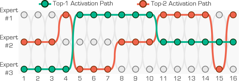
(a) Expert Activation Paths (Beam Number)

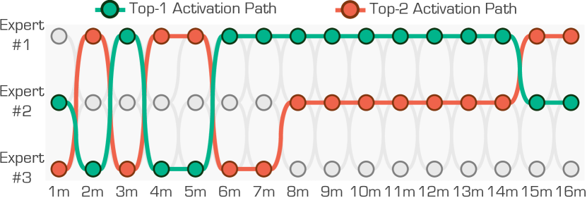
(b) Expert Activation Paths (Distances to Ego)

Figure 7: Visual interpretations of the expert activation paths in CML. The experts are #1 range view, #2 voxel, and #3 point, respectively.

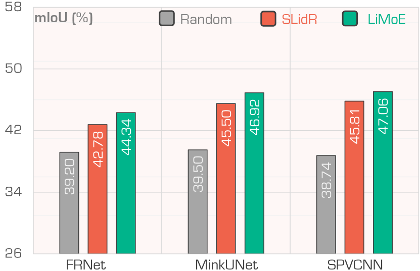
(a) SemanticKITTI

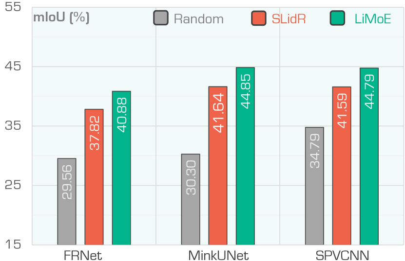
(b) nuScenes

Figure 8: Ablation study on different backbones for downstream tasks. The backbones are initialized with random weights, SLidR [66], and LiMoE, respectively, and fine-tuned on the SemanticKITTI [2] and nuScenes [23] datasets using $1\%$ annotations.

7 Additional Quantitative Results

In this section, we present class-wise LiDAR semantic segmentation results to reinforce the findings and conclusions presented in the main body of the paper.

7.1 Class-Wise Linear Probing Results

Tab. 6 showcases class-wise LiDAR semantic segmentation results on the nuScenes [7, 23] dataset, achieved through pretraining followed by linear probing. The evaluation covers all 16 semantic classes, offering a detailed performance comparison across diverse object categories. LiMoE consistently surpasses single-representation baselines for every class, including challenging categories like “pedestrian”, “bicycle”, and “traffic cone”. These results emphasize the advantage of our approach in utilizing complementary features from range images, sparse voxels, and raw points during the CML stage to capture high-level semantic correlations effectively.

7.2 Class-Wise Fine-Tuning Results

Tab. 7 presents class-wise LiDAR semantic segmentation results on the nuScenes [7, 23] dataset, derived from pretraining followed by fine-tuning with only $1\%$ of the available annotations. The results highlight that LiMoE consistently outperforms single-representation baselines across all classes, with particularly notable gains for dynamic objects such as “pedestrian”, “bicycle”, and “motorcycle”, which often exhibit complex structures. These improvements stem from the SMS stage, where the integration of multiple representations enables the model to capture complementary object attributes, enhancing segmentation performance.

7.3 Extend to Different Backbones

We evaluate the downstream performance of FRNet [83], MinKUNet [15], and SPVCNN [72] across various pretraining strategies, including random initialization, SLidR [66], and LiMoE. Importantly, the downstream fine-tuning does not employ the MoE strategy to combine multiple LiDAR representations, ensuring a fair comparison among the methods. Fine-tuning is conducted on two widely-used datasets, SemanticKITTI [2] and nuScenes [23], with only $1\%$ of the annotations available. As shown in Fig. 8, LiMoE pretraining consistently improves the performance of single-representation methods. This demonstrates the scalability and generalizable feature representations learned during the LiMoE pretraining stage, making it effective for enhancing downstream tasks.

8 Additional Qualitative Results

In this section, we provide additional qualitative examples to visually compare different approaches presented in the main body of the paper.

8.1 Route Activations from CML

LiDAR sensors inherently operate with a fixed number of beams, resulting in a structured arrangement of data points within the captured point clouds. This beam-based configuration provides a natural attribution for the LiDAR point clouds, with each beam contributing a distinct set of points that collectively form a comprehensive 3D representation of the environment. Furthermore, the distance of points from the ego vehicle often correlates with the orientation and elevation of the laser beams. Upper beams are typically designed to detect objects at longer distances, capturing information about the far-field surroundings. In contrast, middle beams are optimized for medium-range detections, while lower beams primarily focus on capturing close-proximity objects [40, 42].

To understand how each LiDAR representation contributes to the fused features within the MoE layer, we conduct a detailed statistical analysis of export selection patterns during the CML stage. Specifically, we examined the activation frequency of each representation – range view, voxel, and point – across varying laser beams and distances from the ego vehicle, measuring their respective contributions to the fused outputs. As depicted in Fig. 7, distinct focus areas emerge for each LiDAR representation, aligning with their inherent strengths. The range view representation shows a higher activation frequency in middle-range regions. The voxel representation demonstrates a significant focus on upper laser beams and far-field regions. The point representation dominates in close-range regions. This analysis underscores the complementary nature of the three representations. The MoE layer dynamically selects the most suitable representation based on the spatial and distance characteristics of the input, enabling a more robust and comprehensive understanding of 3D environments.

8.2 Point-Wise Activation from SMS

SMS supervises the feature learning process by integrating the semantic logits from multiple LiDAR representations with guidance from semantic labels. To illustrate which object attributes each representation focuses on within the LiDAR point clouds, we analyze the contribution of each representation to the semantic logits during the SMS stage.

Specifically, the MoE layer computes a gating score that indicates the relative importance of each representation for individual points. We highlight the most relevant attributes contributed by each representation and project them onto the corresponding point clouds. As shown in Fig. 9, Fig. 10, Fig. 11, and Fig. 12, the range view representation predominantly emphasizes dynamic objects, such as “car”, “truck”, as well as objects in medium-range regions. The voxel representation excels in capturing static background elements, such as “road” and far-field objects within sparse regions. The point representation specializes in intricate details, such as object edges and close-range features, which are crucial for accurate boundary delineation.

This visualization demonstrates the complementary nature of these representations and underscores the effectiveness of SMS in dynamically leveraging their unique strengths. By aligning these diverse features, SMS ensures comprehensive feature learning, leading to improved segmentation performance across varied object types and environmental conditions.

8.3 LiDAR Segmentation Results

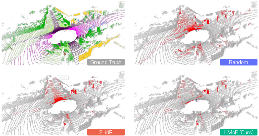
Figure 14: Qualitative assessments of state-of-the-art pretraining methods, pretrained on nuScenes [7] and fine-tuned on SemanticKITTI [2] with $1\%$ annotations. The error maps depict correct and incorrect predictions in gray and red, respectively. Best viewed in colors.

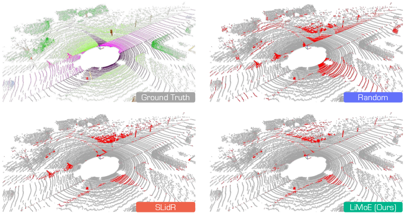
Figure 15: Qualitative assessments of state-of-the-art pretraining methods, pretrained on nuScenes [7] and fine-tuned on SemanticKITTI [2] with $1\%$ annotations. The error maps depict correct and incorrect predictions in gray and red, respectively. Best viewed in colors.

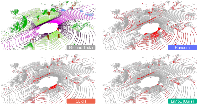
Figure 16: Qualitative assessments of state-of-the-art pretraining methods, pretrained on nuScenes [7] and fine-tuned on SemanticKITTI [2] with $1\%$ annotations. The error maps depict correct and incorrect predictions in gray and red, respectively. Best viewed in colors.

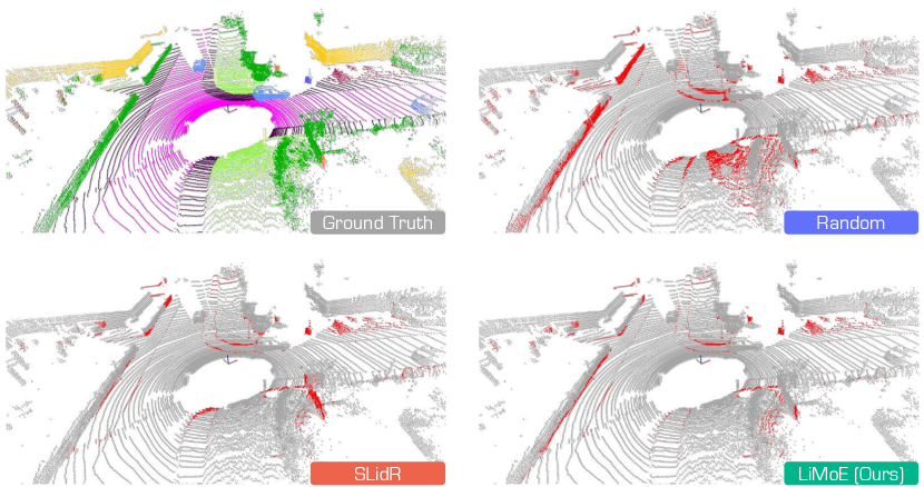
Figure 17: Qualitative assessments of state-of-the-art pretraining methods, pretrained on nuScenes [7] and fine-tuned on SemanticKITTI [2] with $1\%$ annotations. The error maps depict correct and incorrect predictions in gray and red, respectively. Best viewed in colors.

In Fig. 14, Fig. 15, Fig. 16, and Fig. 17, we present qualitative LiDAR segmentation results, highlighting the performance of models pretrained on the nuScenes [92] dataset using various methods and fine-tuned on the SemanticKITTI dataset with $1\%$ of the available annotations. As depicted, LiMoE consistently outperforms single-representation approaches by capturing intricate scene details and achieving a significant reduction in segmentation errors across challenging semantic classes. Notably, it excels in handling dynamic objects such as “pedestrian”, where other methods often struggle. These results highlight the ability of our multi-representation fusion framework to integrate complementary features, leading to more robust and accurate segmentation.

8.4 Cosine Similarity Results

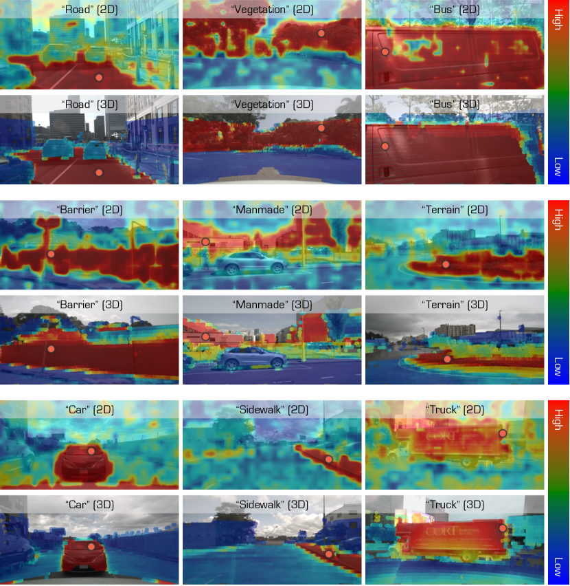
Figure 13: Cosine similarity between the learned features of a query point (denoted as the red dot) and: (1) the features of the image of the same scene (the 1st, 3rd, and 5th rows); and (2) the features of the LiDAR points of the same scene that are projected onto the image (the 2nd, 4th, and 6th rows). Best viewed in colors.

In Fig. 13, we provide additional cosine similarity maps generated during the CML stage. These maps demonstrate the ability of LiMoE to align features from different LiDAR representations, showcasing high semantic correlations across diverse regions of the scene during pretraining. This alignment reflects the effectiveness of our framework in fusing information from range images, sparse voxels, and raw points to capture complementary semantic cues. By fostering strong inter-representation consistency, our method establishes a solid foundation for downstream tasks, improving the performance and reliability of LiDAR-based segmentation systems in real-world scenarios.

9 Public Resources Used

In this section, we acknowledge the use of public resources, during the course of this work.

9.1 Public Codebase Used

We acknowledge the use of the following public codebase, during the course of this work.

• MMEngine Apache License 2.0

• MMCV Apache License 2.0

• MMPretrain Apache License 2.0

• MMDetection Apache License 2.0

• MMDetection3d Apache License 2.0

9.2 Public Datasets Used

We acknowledge the use of the following public datasets, during the course of this work.

• nuScenes CC BY-NC-SA 4.0

• SemanticKITTI CC BY-NC-SA 4.0

• WaymoOpenDataset Waymo Dataset License

• ScribbleKITTI Unknown

• RELLIS-3D CC BY-NC-SA 3.0

• SemanticPOSS CC BY-NC-SA 3.0

• SemanticSTF CC BY-NC-SA 4.0

• SynLiDAR MiT License

• DAPS-3D MiT License

• Synth4D GPL-3.0 License

• Robo3D CC BY-NC-SA 4.0

9.3 Public Implementations Used

We acknowledge the use of the following public implementations, during the course of this work.

• nuscenes-devkit Apache License 2.0

• semantic-kitti-api MIT License

• waymo-open-dataset Apache License 2.0

• SLidR Apache License 2.0

• SuperFlow Apache License 2.0

• FRNet Apache License 2.0

• DINOv2 Apache License 2.0

• torchsparse MIT License

• Conv-LoRA Apache License 2.0

• MoE-LLaVA Apache License 2.0

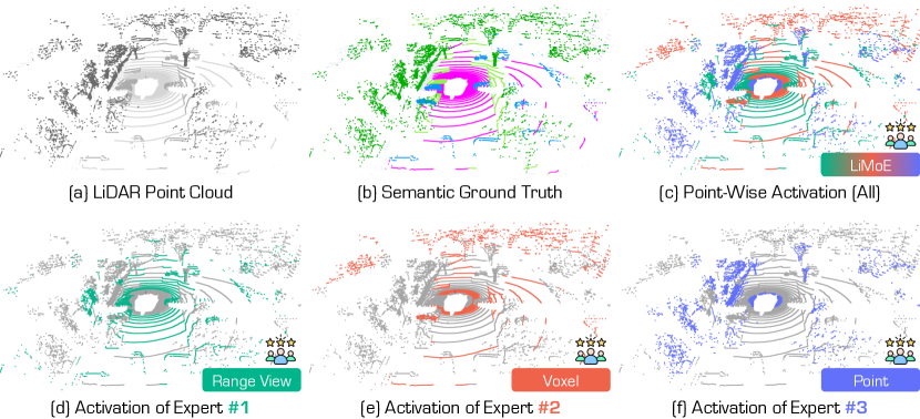
Figure 9: Point-wise top-1 activation path in the SMS stage. It highlights the most activated representation for each point during the SMS stage, illustrating how different representations contribute to semantic segmentation based on spatial and object-specific characteristics. Best viewed in colors.

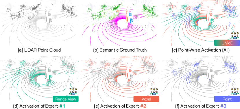
Figure 10: Point-wise top-1 activation path in the SMS stage. It highlights the most activated representation for each point during the SMS stage, illustrating how different representations contribute to semantic segmentation based on spatial and object-specific characteristics. Best viewed in colors.

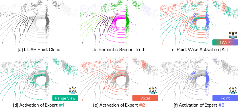
Figure 11: Point-wise top-1 activation path in the SMS stage. It highlights the most activated representation for each point during the SMS stage, illustrating how different representations contribute to semantic segmentation based on spatial and object-specific characteristics. Best viewed in colors.

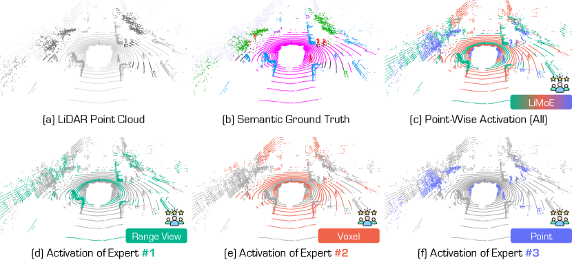
Figure 12: Point-wise top-1 activation path in the SMS stage. It highlights the most activated representation for each point during the SMS stage, illustrating how different representations contribute to semantic segmentation based on spatial and object-specific characteristics. Best viewed in colors.

Table 6: The per-class IoU scores of state-of-the-art pretraining methods pretrained and linear-probed on the nuScenes [7, 23] dataset. All scores are given in percentage (%). The best and 2nd best scores under each group are highlighted in bold and underline.

Method	mIoU	$\blacksquare$ barrier	$\blacksquare$ bicycle	$\blacksquare$ bus	$\blacksquare$ car	$\blacksquare$ construction vehicle	$\blacksquare$ motorcycle	$\blacksquare$ pedestrian	$\blacksquare$ traffic cone	$\blacksquare$ trailer	$\blacksquare$ truck	$\blacksquare$ driveable surface	$\blacksquare$ other flat	$\blacksquare$ sidewalk	$\blacksquare$ terrain	$\blacksquare$ manmade	$\blacksquare$ vegetation
Random	$8.1$	$0.5$	$0.0$	$0.0$	$3.9$	$0.0$	$0.0$	$0.0$	$6.4$	$0.0$	$3.9$	$59.6$	$0.0$	$0.1$	$16.2$	$30.6$	$12.0$
Distill: None
PointContrast [80]	$21.9$	-	-	-	-	-	-	-	-	-	-	-	-	-	-	-	-
DepthContrast [90]	$\mathbf{22.1}$	-	-	-	-	-	-	-	-	-	-	-	-	-	-	-	-
ALSO [6]	-	-	-	-	-	-	-	-	-	-	-	-	-	-	-	-	-
BEVContrast [67]	-	-	-	-	-	-	-	-	-	-	-	-	-	-	-	-	-
Distill: ResNet-50
PPKT [49]	$35.9$	-	-	-	-	-	-	-	-	-	-	-	-	-	-	-	-
SLidR [66]	$39.2$	$44.2$	$0.0$	$\mathbf{30.8}$	$60.2$	$15.1$	$22.4$	$47.2$	$27.7$	$16.3$	$34.3$	$80.6$	$21.8$	$35.2$	$48.1$	$71.0$	$71.9$
ST-SLidR [52]	$40.5$	-	-	-	-	-	-	-	-	-	-	-	-	-	-	-	-
TriCC [58]	$38.0$	-	-	-	-	-	-	-	-	-	-	-	-	-	-	-	-
Seal [47]	$45.0$	$\mathbf{54.7}$	$\mathbf{5.9}$	$30.6$	$\mathbf{61.7}$	$\mathbf{18.9}$	$\mathbf{28.8}$	$\mathbf{48.1}$	$\mathbf{31.0}$	$\mathbf{22.1}$	$\mathbf{39.5}$	$\mathbf{83.8}$	$\mathbf{35.4}$	$\mathbf{46.7}$	$\mathbf{56.9}$	$\mathbf{74.7}$	$\mathbf{74.7}$
CSC [9]	$\mathbf{46.0}$	-	-	-	-	-	-	-	-	-	-	-	-	-	-	-	-
HVDistill [88]	$39.5$	-	-	-	-	-	-	-	-	-	-	-	-	-	-	-	-
Distill: ViT-S
PPKT [49]	$38.6$	$43.8$	$0.0$	$31.2$	$53.1$	$15.2$	$0.0$	$42.2$	$16.5$	$18.3$	$33.7$	$79.1$	$37.2$	$45.2$	$52.7$	$75.6$	$74.3$
SLidR [66]	$44.7$	$45.0$	$8.2$	$34.8$	$58.6$	$23.4$	$40.2$	$43.8$	$19.0$	$22.9$	$40.9$	$82.7$	$38.3$	$47.6$	$53.9$	$77.8$	$77.9$
+ LiMoE	$45.8$	$46.2$	$\mathbf{8.5}$	$36.2$	$59.4$	$\mathbf{23.6}$	$\mathbf{41.7}$	$47.2$	$20.7$	$24.1$	$43.2$	$83.9$	$38.7$	$\mathbf{48.1}$	$55.3$	$\mathbf{78.0}$	$78.6$
Seal [47]	$45.2$	$48.9$	$8.4$	$30.7$	$\mathbf{68.1}$	$17.5$	$37.7$	$57.7$	$17.9$	$20.9$	$40.4$	$83.8$	$36.6$	$44.2$	$54.5$	$76.2$	$\mathbf{79.3}$
SuperFlow [84]	$46.4$	$49.8$	$6.8$	$45.9$	$63.4$	$18.5$	$31.0$	$60.3$	$28.1$	$25.4$	$47.4$	$86.2$	$38.4$	$47.4$	$56.7$	$74.9$	$77.8$
+ LiMoE	$\mathbf{48.2}$	$\mathbf{50.4}$	$7.9$	$\mathbf{46.7}$	$65.1$	$19.2$	$32.1$	$\mathbf{61.5}$	$\mathbf{29.5}$	$\mathbf{26.7}$	$\mathbf{48.3}$	$\mathbf{86.5}$	$\mathbf{39.1}$	$48.0$	$\mathbf{57.4}$	$75.1$	$78.4$
Distill: ViT-B
PPKT [49]	$40.0$	$29.6$	$0.0$	$30.7$	$55.8$	$6.3$	$22.4$	$56.7$	$18.1$	$24.3$	$42.7$	$82.3$	$33.2$	$45.1$	$53.4$	$71.3$	$75.7$
SLidR [66]	$45.4$	$46.7$	$7.8$	$46.5$	$58.7$	$23.9$	$34.0$	$47.8$	$17.1$	$23.7$	$41.7$	$83.4$	$39.4$	$47.0$	$54.6$	$76.6$	$77.8$
+ LiMoE	$46.6$	$48.2$	$8.6$	$47.1$	$61.1$	$\mathbf{25.0}$	$35.3$	$48.6$	$18.4$	$\mathbf{24.4}$	$43.4$	$84.6$	$\mathbf{39.9}$	$47.4$	$56.9$	$\mathbf{77.4}$	$78.9$
Seal [47]	$46.6$	$\mathbf{49.3}$	$8.2$	$35.1$	$\mathbf{70.8}$	$22.1$	$41.7$	$57.4$	$15.2$	$21.6$	$42.6$	$84.5$	$38.1$	$46.8$	$55.4$	$77.2$	$\mathbf{79.5}$
SuperFlow [84]	$47.7$	$45.8$	$12.4$	$52.6$	$67.9$	$17.2$	$40.8$	$59.5$	$25.4$	$21.0$	$47.6$	$85.8$	$37.2$	$48.4$	$56.6$	$76.2$	$78.2$
+ LiMoE	$\mathbf{49.1}$	$46.8$	$\mathbf{13.1}$	$\mathbf{53.9}$	$68.4$	$19.2$	$\mathbf{42.2}$	$\mathbf{59.9}$	$\mathbf{27.5}$	$21.7$	$\mathbf{48.3}$	$\mathbf{85.9}$	$38.2$	$\mathbf{49.0}$	$\mathbf{57.1}$	$76.3$	$78.8$
Distill: ViT-L
PPKT [49]	$41.6$	$30.5$	$0.0$	$32.0$	$57.3$	$8.7$	$24.0$	$58.1$	$19.5$	$\mathbf{24.9}$	$44.1$	$83.1$	$34.5$	$45.9$	$55.4$	$72.5$	$76.4$
SLidR [66]	$45.7$	$46.9$	$6.9$	$44.9$	$60.8$	$22.7$	$40.6$	$44.7$	$17.4$	$23.0$	$40.4$	$83.6$	$39.9$	$47.8$	$55.2$	$78.1$	$78.3$
+ LiMoE	$47.4$	$48.7$	$9.2$	$46.7$	$62.7$	$\mathbf{24.2}$	$42.1$	$46.2$	$19.7$	$24.4$	$43.2$	$\mathbf{85.3}$	$\mathbf{41.6}$	$\mathbf{49.5}$	$57.4$	$\mathbf{78.7}$	$79.3$
Seal [47]	$46.8$	$53.1$	$6.9$	$35.0$	$65.0$	$22.0$	$46.1$	$\mathbf{59.2}$	$16.2$	$23.0$	$41.8$	$84.7$	$35.8$	$46.6$	$55.5$	$78.4$	$\mathbf{79.8}$
SuperFlow [84]	$48.0$	$52.3$	$12.7$	$46.5$	$64.7$	$21.4$	$44.9$	$56.2$	$26.7$	$19.9$	$43.2$	$84.2$	$38.1$	$47.4$	$56.9$	$76.0$	$79.2$
+ LiMoE	$\mathbf{49.4}$	$\mathbf{54.4}$	$\mathbf{14.4}$	$\mathbf{47.9}$	$\mathbf{66.1}$	$23.9$	$\mathbf{46.7}$	$57.2$	$\mathbf{27.9}$	$20.8$	$\mathbf{44.8}$	$85.0$	$39.6$	$48.1$	$\mathbf{58.2}$	$76.5$	$79.6$

Table 7: The per-class IoU scores of state-of-the-art pretraining methods pretrained and fine-tuned on the nuScenes [7, 23] dataset with $1\%$ annotations. All scores are given in percentage (%). The best and 2nd best scores under each group are highlighted in bold and underline.

Method	mIoU	$\blacksquare$ barrier	$\blacksquare$ bicycle	$\blacksquare$ bus	$\blacksquare$ car	$\blacksquare$ construction vehicle	$\blacksquare$ motorcycle	$\blacksquare$ pedestrian	$\blacksquare$ traffic cone	$\blacksquare$ trailer	$\blacksquare$ truck	$\blacksquare$ driveable surface	$\blacksquare$ other flat	$\blacksquare$ sidewalk	$\blacksquare$ terrain	$\blacksquare$ manmade	$\blacksquare$ vegetation
Random	$30.3$	$0.0$	$0.0$	$8.1$	$65.0$	$0.1$	$6.6$	$21.0$	$9.0$	$9.3$	$25.8$	$89.5$	$14.8$	$41.7$	$48.7$	$72.4$	$73.3$
Distill: None
PointContrast [80]	$32.5$	$0.0$	$1.0$	$5.6$	$67.4$	$0.0$	$3.3$	$31.6$	$5.6$	$12.1$	$30.8$	$\mathbf{91.7}$	$21.9$	$\mathbf{48.4}$	$50.8$	$75.0$	$74.6$
DepthContrast [90]	$31.7$	$0.0$	$0.6$	$6.5$	$64.7$	$0.2$	$\mathbf{5.1}$	$29.0$	$\mathbf{9.5}$	$12.1$	$29.9$	$90.3$	$17.8$	$44.4$	$49.5$	$73.5$	$74.0$
ALSO [6]	$37.7$	-	-	-	-	-	-	-	-	-	-	-	-	-	-	-	-
BEVContrast [67]	$\mathbf{37.9}$	$0.0$	$\mathbf{1.3}$	$\mathbf{32.6}$	$\mathbf{74.3}$	$\mathbf{1.1}$	$0.9$	$\mathbf{41.3}$	$8.1$	$\mathbf{24.1}$	$\mathbf{40.9}$	$89.8$	$\mathbf{36.2}$	$44.0$	$\mathbf{52.1}$	$\mathbf{79.9}$	$\mathbf{79.7}$
Distill: ResNet-50
PPKT [49]	$37.8$	$0.0$	$2.2$	$20.7$	$75.4$	$1.2$	$13.2$	$45.6$	$8.5$	$17.5$	$38.4$	$92.5$	$19.2$	$52.3$	$56.8$	$80.1$	$80.9$
SLidR [66]	$38.8$	$0.0$	$1.8$	$15.4$	$73.1$	$1.9$	$19.9$	$47.2$	$17.1$	$14.5$	$34.5$	$92.0$	$27.1$	$53.6$	$61.0$	$79.8$	$82.3$
ST-SLidR [52]	$40.8$	-	-	-	-	-	-	-	-	-	-	-	-	-	-	-	-
TriCC [58]	$41.2$	-	-	-	-	-	-	-	-	-	-	-	-	-	-	-	-
Seal [47]	$45.8$	$0.0$	$\mathbf{9.4}$	$32.6$	$\mathbf{77.5}$	$\mathbf{10.4}$	$28.0$	$53.0$	$25.0$	$\mathbf{30.9}$	$\mathbf{49.7}$	$\mathbf{94.0}$	$\mathbf{33.7}$	$\mathbf{60.1}$	$59.6$	$\mathbf{83.9}$	$83.4$
CSC [9]	$\mathbf{47.0}$	$0.0$	$0.0$	$\mathbf{58.7}$	$74.0$	$0.1$	$\mathbf{40.9}$	$\mathbf{58.9}$	$\mathbf{31.8}$	$23.7$	$45.1$	$92.5$	$33.0$	$56.4$	$\mathbf{62.4}$	$81.6$	$\mathbf{84.2}$
HVDistill [88]	$42.7$	-	-	-	-	-	-	-	-	-	-	-	-	-	-	-	-
Distill: ViT-S
PPKT [49]	$40.6$	$0.0$	$0.0$	$25.2$	$73.5$	$9.1$	$6.9$	$51.4$	$8.6$	$11.3$	$31.1$	$93.2$	$\mathbf{41.7}$	$58.3$	$64.0$	$82.0$	$82.6$
SLidR [66]	$41.2$	$0.0$	$0.0$	$26.6$	$72.0$	$12.4$	$15.8$	$51.4$	$22.9$	$11.7$	$35.3$	$92.9$	$36.3$	$58.7$	$63.6$	$81.2$	$82.3$
+ LiMoE	$46.8$	$20.6$	$4.2$	$\mathbf{29.7}$	$74.7$	$16.9$	$24.6$	$55.7$	$28.3$	$19.5$	$41.5$	$93.8$	$41.0$	$\mathbf{62.4}$	$\mathbf{67.3}$	$82.6$	$\mathbf{85.2}$
Seal [47]	$44.3$	$20.0$	$0.0$	$19.4$	$74.7$	$10.6$	$\mathbf{45.7}$	$60.3$	$\mathbf{29.2}$	$17.4$	$38.1$	$93.2$	$26.0$	$58.8$	$64.5$	$81.9$	$81.9$
SuperFlow [84]	$47.8$	$38.2$	$1.8$	$25.8$	$79.0$	$15.3$	$43.6$	$60.3$	$0.0$	$28.4$	$55.4$	$93.7$	$28.8$	$59.1$	$59.9$	$83.5$	$83.1$
+ LiMoE	$\mathbf{49.6}$	$\mathbf{39.9}$	$\mathbf{4.6}$	$27.3$	$\mathbf{80.2}$	$\mathbf{17.1}$	$45.4$	$\mathbf{61.2}$	$6.2$	$\mathbf{29.5}$	$\mathbf{58.4}$	$\mathbf{94.0}$	$34.2$	$62.3$	$64.6$	$\mathbf{84.1}$	$84.5$
Distill: ViT-B
PPKT [49]	$40.9$	$0.0$	$0.0$	$24.5$	$73.5$	$12.2$	$7.0$	$51.0$	$13.5$	$15.4$	$36.3$	$93.1$	$40.4$	$59.2$	$63.5$	$81.7$	$82.2$
SLidR [66]	$41.6$	$0.0$	$0.0$	$26.7$	$73.4$	$10.3$	$16.9$	$51.3$	$23.3$	$12.7$	$38.1$	$93.0$	$37.7$	$58.8$	$63.4$	$81.6$	$82.7$
+ LiMoE	$46.9$	$22.7$	$2.6$	$28.3$	$75.4$	$\mathbf{13.5}$	$27.8$	$55.0$	$\mathbf{28.5}$	$22.2$	$40.6$	$93.7$	$\mathbf{42.3}$	$61.9$	$\mathbf{66.8}$	$83.1$	$\mathbf{85.4}$
Seal [47]	$46.0$	$\mathbf{43.0}$	$0.0$	$26.7$	$81.3$	$9.9$	$41.3$	$56.2$	$0.0$	$21.7$	$51.6$	$93.6$	$\mathbf{42.3}$	$62.8$	$64.7$	$82.6$	$82.7$
SuperFlow [84]	$48.1$	$39.1$	$0.9$	$30.0$	$80.7$	$10.3$	$47.1$	$59.5$	$5.1$	$27.6$	$55.4$	$93.7$	$29.1$	$61.1$	$63.5$	$82.7$	$83.6$
+ LiMoE	$\mathbf{50.2}$	$41.5$	$\mathbf{3.8}$	$\mathbf{32.2}$	$\mathbf{81.7}$	$12.9$	$\mathbf{49.3}$	$\mathbf{61.1}$	$7.3$	$\mathbf{29.3}$	$\mathbf{57.8}$	$\mathbf{94.2}$	$35.1$	$\mathbf{62.9}$	$65.4$	$\mathbf{84.0}$	$84.8$
Distill: ViT-L
PPKT [49]	$42.1$	$0.0$	$0.0$	$24.4$	$78.8$	$15.1$	$9.2$	$54.2$	$14.3$	$12.9$	$39.1$	$92.9$	$37.8$	$59.8$	$64.9$	$82.3$	$83.6$
SLidR [66]	$42.8$	$0.0$	$0.0$	$23.9$	$78.8$	$15.2$	$20.9$	$55.0$	$28.0$	$17.4$	$41.4$	$92.2$	$41.2$	$58.0$	$64.0$	$81.8$	$82.7$
+ LiMoE	$46.9$	$21.6$	$1.6$	$25.2$	$80.1$	$17.3$	$28.0$	$56.4$	$\mathbf{28.3}$	$18.6$	$43.1$	$92.7$	$\mathbf{41.7}$	$60.9$	$\mathbf{65.5}$	$83.8$	$\mathbf{85.6}$
Seal [47]	$46.3$	$41.8$	$0.0$	$23.8$	$81.4$	$17.7$	$46.3$	$58.6$	$0.0$	$23.4$	$54.7$	$93.8$	$41.4$	$62.5$	$65.0$	$\underline{83.9}$	$83.8$
SuperFlow [84]	$50.0$	$44.5$	$0.9$	$22.4$	$80.8$	$17.1$	$50.2$	$60.9$	$21.0$	$25.1$	$55.1$	$93.9$	$35.8$	$61.5$	$62.6$	$83.7$	$83.7$
+ LiMoE	$\mathbf{51.4}$	$\mathbf{45.3}$	$\mathbf{4.1}$	$\mathbf{25.3}$	$\mathbf{82.2}$	$\mathbf{18.4}$	$\mathbf{52.5}$	$\mathbf{61.8}$	$22.3$	$\mathbf{26.4}$	$\mathbf{56.2}$	$\mathbf{94.3}$	$37.6$	$\mathbf{63.3}$	$63.9$	$\mathbf{84.4}$	$85.0$

References

- Achanta et al. [2012] Radhakrishna Achanta, Appu Shaji, Kevin Smith, Aurelien Lucchi, Pascal Fua, and Sabine Süsstrunk. Slic superpixels compared to state-of-the-art superpixel methods. IEEE Transactions on Pattern Analysis and Machine Intelligence, 34(11):2274–2282, 2012.
- Behley et al. [2019] Jens Behley, Martin Garbade, Andres Milioto, Jan Quenzel, Sven Behnke, Cyrill Stachniss, and Jurgen Gall. Semantickitti: A dataset for semantic scene understanding of lidar sequences. In IEEE/CVF International Conference on Computer Vision, pages 9297–9307, 2019.
- Bengio et al. [2013] Yoshua Bengio, Aaron Courville, and Pascal Vincent. Representation learning: A review and new perspectives. IEEE Transactions on Pattern Analysis and Machine Intelligence, 35(8):1798–1828, 2013.
- Berman et al. [2018] Maxim Berman, Amal Rannen Triki, and Matthew B Blaschko. The lovász-softmax loss: A tractable surrogate for the optimization of the intersection-over-union measure in neural networks. In IEEE/CVF Conference on Computer Vision and Pattern Recognition, pages 4413–4421, 2018.
- Bijelic et al. [2020] Mario Bijelic, Tobias Gruber, Fahim Mannan, Florian Kraus, Werner Ritter, Klaus Dietmayer, and Felix Heide. Seeing through fog without seeing fog: Deep multimodal sensor fusion in unseen adverse weather. In Proceedings of the IEEE/CVF Conference on Computer Vision and Pattern Recognition, pages 11682–11692, 2020.
- Boulch et al. [2023] Alexandre Boulch, Corentin Sautier, Björn Michele, Gilles Puy, and Renaud Marlet. Also: Automotive lidar self-supervision by occupancy estimation. In IEEE/CVF Conference on Computer Vision and Pattern Recognition, pages 13455–13465, 2023.
- Caesar et al. [2020] Holger Caesar, Varun Bankiti, Alex H Lang, Sourabh Vora, Venice Erin Liong, Qiang Xu, Anush Krishnan, Yu Pan, Giancarlo Baldan, and Oscar Beijbom. nuscenes: A multimodal dataset for autonomous driving. In IEEE/CVF Conference on Computer Vision and Pattern Recognition, pages 11621–11631, 2020.
- Cai et al. [2024] Weilin Cai, Juyong Jiang, Fan Wang, Jing Tang, Sunghun Kim, and Jiayi Huang. A survey on mixture of experts. arXiv preprint arXiv:2407.06204, 2024.
- Chen et al. [2024a] Haoming Chen, Zhizhong Zhang, Yanyun Qu, Ruixin Zhang, Xin Tan, and Yuan Xie. Building a strong pre-training baseline for universal 3d large-scale perception. In IEEE/CVF Conference on Computer Vision and Pattern Recognition, pages 19925–19935, 2024a.
- Chen et al. [2024b] Li Chen, Penghao Wu, Kashyap Chitta, Bernhard Jaeger, Andreas Geiger, and Hongyang Li. End-to-end autonomous driving: Challenges and frontiers. IEEE Transactions on Pattern Analysis and Machine Intelligence, 2024b.
- Chen et al. [2021] Qi Chen, Sourabh Vora, and Oscar Beijbom. Polarstream: Streaming lidar object detection and segmentation with polar pillars. In Advances in Neural Information Processing Systems, 2021.
- Chen et al. [2020] Ting Chen, Simon Kornblith, Mohammad Norouzi, and Geoffrey Hinton. A simple framework for contrastive learning of visual representations. In International conference on machine learning, pages 1597–1607, 2020.
- Chen et al. [2023] Tianlong Chen, Xuxi Chen, Xianzhi Du, Abdullah Rashwan, Fan Yang, Huizhong Chen, Zhangyang Wang, and Yeqing Li. Adamv-moe: Adaptive multi-task vision mixture-of-experts. In IEEE/CVF International Conference on Computer Vision, pages 17346–17357, 2023.
- Chowdhury et al. [2023] Mohammed Nowaz Rabbani Chowdhury, Shuai Zhang, Meng Wang, Sijia Liu, and Pin-Yu Chen. Patch-level routing in mixture-of-experts is provably sample-efficient for convolutional neural networks. In International Conference on Machine Learning, pages 6074–6114, 2023.
- Choy et al. [2019] Christopher Choy, JunYoung Gwak, and Silvio Savarese. 4d spatio-temporal convnets: Minkowski convolutional neural networks. In IEEE/CVF Conference on Computer Vision and Pattern Recognition, pages 3075–3084, 2019.
- Contributors [2020] MMDetection3D Contributors. MMDetection3D: OpenMMLab next-generation platform for general 3D object detection. https://github.com/open-mmlab/mmdetection3d, 2020.
- Contributors [2022] Spconv Contributors. Spconv: Spatially sparse convolution library. https://github.com/traveller59/spconv, 2022.
- Cortinhal et al. [2020] Tiago Cortinhal, George Tzelepis, and Eren Erdal Aksoy. Salsanext: Fast, uncertainty-aware semantic segmentation of lidar point clouds. In International Symposium on Visual Computing, pages 207–222, 2020.
- Dosovitskiy et al. [2021] Alexey Dosovitskiy, Lucas Beyer, Alexander Kolesnikov, Dirk Weissenborn, Xiaohua Zhai, Thomas Unterthiner, Mostafa Dehghani, Matthias Minderer, Georg Heigold, Sylvain Gelly, et al. An image is worth 16x16 words: Transformers for image recognition at scale. In International Conference on Learning Representations, 2021.
- Du et al. [2022] Nan Du, Yanping Huang, Andrew M Dai, Simon Tong, Dmitry Lepikhin, Yuanzhong Xu, Maxim Krikun, Yanqi Zhou, Adams Wei Yu, Orhan Firat, et al. Glam: Efficient scaling of language models with mixture-of-experts. In International Conference on Machine Learning, pages 5547–5569, 2022.
- Fedus et al. [2022a] William Fedus, Jeff Dean, and Barret Zoph. A review of sparse expert models in deep learning. arXiv preprint arXiv:2209.01667, 2022a.
- Fedus et al. [2022b] William Fedus, Barret Zoph, and Noam Shazeer. Switch transformers: Scaling to trillion parameter models with simple and efficient sparsity. Journal of Machine Learning Research, 23(120):1–39, 2022b.
- Fong et al. [2022] Whye Kit Fong, Rohit Mohan, Juana Valeria Hurtado, Lubing Zhou, Holger Caesar, Oscar Beijbom, and Abhinav Valada. Panoptic nuscenes: A large-scale benchmark for lidar panoptic segmentation and tracking. IEEE Robotics and Automation Letters, 7:3795–3802, 2022.
- Gao et al. [2021] Biao Gao, Yancheng Pan, Chengkun Li, Sibo Geng, and Huijing Zhao. Are we hungry for 3d lidar data for semantic segmentation? a survey of datasets and methods. IEEE Transactions on Intelligent Transportation Systems, 23(7):6063–6081, 2021.
- Geiger et al. [2012] Andreas Geiger, Philip Lenz, and Raquel Urtasun. Are we ready for autonomous driving? the kitti vision benchmark suite. In IEEE/CVF Conference on Computer Vision and Pattern Recognition, pages 3354–3361, 2012.
- Hao et al. [2024] Xiaoshuai Hao, Mengchuan Wei, Yifan Yang, Haimei Zhao, Hui Zhang, Yi Zhou, Qiang Wang, Weiming Li, Lingdong Kong, and Jing Zhang. Is your hd map constructor reliable under sensor corruptions? In Advances in Neural Information Processing Systems, 2024.
- He et al. [2016] Kaiming He, Xiangyu Zhang, Shaoqing Ren, and Jian Sun. Deep residual learning for image recognition. In IEEE/CVF Conference on Computer Vision and Pattern Recognition, pages 770–778, 2016.
- He et al. [2020] Kaiming He, Haoqi Fan, Yuxin Wu, Saining Xie, and Ross Girshick. Momentum contrast for unsupervised visual representation learning. In IEEE/CVF Conference on Computer Vision and Pattern Recognition, pages 9729–9738, 2020.
- He et al. [2022] Kaiming He, Xinlei Chen, Saining Xie, Yanghao Li, Piotr Dollár, and Ross Girshick. Masked autoencoders are scalable vision learners. In IEEE/CVF Conference on Computer Vision and Pattern Recognition, pages 16000–16009, 2022.
- Hong et al. [2021] Fangzhou Hong, Hui Zhou, Xinge Zhu, Hongsheng Li, and Ziwei Liu. Lidar-based panoptic segmentation via dynamic shifting network. In IEEE/CVF Conference on Computer Vision and Pattern Recognition, pages 13090–13099, 2021.
- Hong et al. [2024] Fangzhou Hong, Lingdong Kong, Hui Zhou, Xinge Zhu, Hongsheng Li, and Ziwei Liu. Unified 3d and 4d panoptic segmentation via dynamic shifting networks. IEEE Transactions on Pattern Analysis and Machine Intelligence, 46(5):3480–3495, 2024.
- Hu et al. [2020] Qingyong Hu, Bo Yang, Linhai Xie, Stefano Rosa, Yulan Guo, Zhihua Wang, Niki Trigoni, and Andrew Markham. Randla-net: Efficient semantic segmentation of large-scale point clouds. In IEEE/CVF Conference on Computer Vision and Pattern Recognition, pages 11108–11117, 2020.
- Hwang et al. [2023] Changho Hwang, Wei Cui, Yifan Xiong, Ziyue Yang, Ze Liu, Han Hu, Zilong Wang, Rafael Salas, Jithin Jose, Prabhat Ram, et al. Tutel: Adaptive mixture-of-experts at scale. Proceedings of Machine Learning and Systems, 5:269–287, 2023.
- Jiang et al. [2021] Peng Jiang, Philip Osteen, Maggie Wigness, and Srikanth Saripalli. Rellis-3d dataset: Data, benchmarks and analysis. In IEEE International Conference on Robotics and Automation, pages 1110–1116, 2021.
- Jiang and Shen [2024] Yufeng Jiang and Yiqing Shen. M4oe: A foundation model for medical multimodal image segmentation with mixture of experts. In International Conference on Medical Image Computing and Computer-Assisted Intervention, pages 621–631, 2024.
- Kirillov et al. [2023] Alexander Kirillov, Eric Mintun, Nikhila Ravi, Hanzi Mao, Chloe Rolland, Laura Gustafson, Tete Xiao, Spencer Whitehead, Alexander C Berg, Wan-Yen Lo, et al. Segment anything. In IEEE/CVF International Conference on Computer Vision, pages 4015–4026, 2023.
- Klokov et al. [2023] Alexey A Klokov, Di Un Pak, Aleksandr Khorin, Dmitry A Yudin, Leon Kochiev, Vladimir D Luchinskiy, and Vitaly D Bezuglyj. Daps3d: Domain adaptive projective segmentation of 3d lidar point clouds. IEEE Access, 11:79341–79356, 2023.
- Kong et al. [2023a] Lingdong Kong, Youquan Liu, Runnan Chen, Yuexin Ma, Xinge Zhu, Yikang Li, Yuenan Hou, Yu Qiao, and Ziwei Liu. Rethinking range view representation for lidar segmentation. In IEEE/CVF International Conference on Computer Vision, pages 228–240, 2023a.
- Kong et al. [2023b] Lingdong Kong, Youquan Liu, Xin Li, Runnan Chen, Wenwei Zhang, Jiawei Ren, Liang Pan, Kai Chen, and Ziwei Liu. Robo3d: Towards robust and reliable 3d perception against corruptions. In IEEE/CVF International Conference on Computer Vision, pages 19994–20006, 2023b.
- Kong et al. [2023c] Lingdong Kong, Jiawei Ren, Liang Pan, and Ziwei Liu. Lasermix for semi-supervised lidar semantic segmentation. In IEEE/CVF Conference on Computer Vision and Pattern Recognition, pages 21705–21715, 2023c.
- Kong et al. [2024a] Lingdong Kong, Shaoyuan Xie, Hanjiang Hu, Yaru Niu, Wei Tsang Ooi, Benoit R. Cottereau, Lai Xing Ng, Yuexin Ma, Wenwei Zhang, Liang Pan, Kai Chen, Ziwei Liu, Weichao Qiu, Wei Zhang, Xu Cao, Hao Lu, Ying-Cong Chen, Caixin Kang, Xinning Zhou, Chengyang Ying, Wentao Shang, Xingxing Wei, Yinpeng Dong, Bo Yang, Shengyin Jiang, Zeliang Ma, Dengyi Ji, Haiwen Li, Xingliang Huang, Yu Tian, Genghua Kou, Fan Jia, Yingfei Liu, Tiancai Wang, Ying Li, Xiaoshuai Hao, Yifan Yang, Hui Zhang, Mengchuan Wei, Yi Zhou, Haimei Zhao, Jing Zhang, Jinke Li, Xiao He, Xiaoqiang Cheng, Bingyang Zhang, Lirong Zhao, Dianlei Ding, Fangsheng Liu, Yixiang Yan, Hongming Wang, Nanfei Ye, Lun Luo, Yubo Tian, Yiwei Zuo, Zhe Cao, Yi Ren, Yunfan Li, Wenjie Liu, Xun Wu, Yifan Mao, Ming Li, Jian Liu, Jiayang Liu, Zihan Qin, Cunxi Chu, Jialei Xu, Wenbo Zhao, Junjun Jiang, Xianming Liu, Ziyan Wang, Chiwei Li, Shilong Li, Chendong Yuan, Songyue Yang, Wentao Liu, Peng Chen, Bin Zhou, Yubo Wang, Chi Zhang, Jianhang Sun, Hai Chen, Xiao Yang, Lizhong Wang, Dongyi Fu, Yongchun Lin, Huitong Yang, Haoang Li, Yadan Luo, Xianjing Cheng, and Yong Xu. The robodrive challenge: Drive anytime anywhere in any condition. arXiv preprint arXiv:2405.08816, 2024a.
- Kong et al. [2024b] Lingdong Kong, Xiang Xu, Jiawei Ren, Wenwei Zhang, Liang Pan, Kai Chen, Wei Tsang Ooi, and Ziwei Liu. Multi-modal data-efficient 3d scene understanding for autonomous driving. arXiv preprint arXiv:2405.05258, 2024b.
- Li et al. [2024] Li Li, Hubert PH Shum, and Toby P Breckon. Rapid-seg: Range-aware pointwise distance distribution networks for 3d lidar segmentation. In European Conference on Computer Vision, pages 222–241, 2024.
- Lin et al. [2024] Bin Lin, Zhenyu Tang, Yang Ye, Jiaxi Cui, Bin Zhu, Peng Jin, Jinfa Huang, Junwu Zhang, Yatian Pang, Munan Ning, et al. Moe-llava: Mixture of experts for large vision-language models. arXiv preprint arXiv:2401.15947, 2024.
- Liong et al. [2020] Venice Erin Liong, Thi Ngoc Tho Nguyen, Sergi Widjaja, Dhananjai Sharma, and Zhuang Jie Chong. Amvnet: Assertion-based multi-view fusion network for lidar semantic segmentation. arXiv preprint arXiv:2012.04934, 2020.
- Liu et al. [2023a] Youquan Liu, Runnan Chen, Xin Li, Lingdong Kong, Yuchen Yang, Zhaoyang Xia, Yeqi Bai, Xinge Zhu, Yuexin Ma, Yikang Li, et al. Uniseg: A unified multi-modal lidar segmentation network and the openpcseg codebase. In IEEE/CVF International Conference on Computer Vision, pages 21662–21673, 2023a.
- Liu et al. [2023b] Youquan Liu, Lingdong Kong, Jun Cen, Runnan Chen, Wenwei Zhang, Liang Pan, Kai Chen, and Ziwei Liu. Segment any point cloud sequences by distilling vision foundation models. In Advances in Neural Information Processing Systems, pages 37193–37229, 2023b.
- Liu et al. [2024] Youquan Liu, Lingdong Kong, Xiaoyang Wu, Runnan Chen, Xin Li, Liang Pan, Ziwei Liu, and Yuexin Ma. Multi-space alignments towards universal lidar segmentation. In IEEE/CVF Conference on Computer Vision and Pattern Recognition, pages 14648–14661, 2024.
- Liu et al. [2021] Yueh-Cheng Liu, Yu-Kai Huang, Hung-Yueh Chiang, Hung-Ting Su, Zhe-Yu Liu, Chin-Tang Chen, Ching-Yu Tseng, and Winston H Hsu. Learning from 2d: Contrastive pixel-to-point knowledge transfer for 3d pretraining. arXiv preprint arXiv:2104.0468, 2021.
- Loshchilov and Hutter [2018] Ilya Loshchilov and Frank Hutter. Decoupled weight decay regularization. In International Conference on Learning Representations, 2018.
- Ma et al. [2024] Yuexin Ma, Tai Wang, Xuyang Bai, Huitong Yang, Yuenan Hou, Yaming Wang, Yu Qiao, Ruigang Yang, Dinesh Manocha, and Xinge Zhu. Vision-centric bev perception: A survey. IEEE Transactions on Pattern Analysis and Machine Intelligence, 2024.
- Mahmoud et al. [2023] Anas Mahmoud, Jordan SK Hu, Tianshu Kuai, Ali Harakeh, Liam Paull, and Steven L Waslander. Self-supervised image-to-point distillation via semantically tolerant contrastive loss. In IEEE/CVF Conference on Computer Vision and Pattern Recognition, pages 7102–7110, 2023.
- Masoudnia and Ebrahimpour [2014] Saeed Masoudnia and Reza Ebrahimpour. Mixture of experts: a literature survey. Artificial Intelligence Review, 42:275–293, 2014.
- Milioto et al. [2019] Andres Milioto, Ignacio Vizzo, Jens Behley, and Cyrill Stachniss. Rangenet++: Fast and accurate lidar semantic segmentation. In IEEE/RSJ International Conference on Intelligent Robots and Systems, pages 4213–4220, 2019.
- Muhammad et al. [2020] Khan Muhammad, Amin Ullah, Jaime Lloret, Javier Del Ser, and Victor Hugo C de Albuquerque. Deep learning for safe autonomous driving: Current challenges and future directions. IEEE Transactions on Intelligent Transportation Systems, 22(7):4316–4336, 2020.
- Oquab et al. [2023] Maxime Oquab, Timothée Darcet, Théo Moutakanni, Huy Vo, Marc Szafraniec, Vasil Khalidov, Pierre Fernandez, Daniel Haziza, Francisco Massa, Alaaeldin El-Nouby, et al. Dinov2: Learning robust visual features without supervision. arXiv preprint arXiv:2304.07193, 2023.
- Pan et al. [2020] Yancheng Pan, Biao Gao, Jilin Mei, Sibo Geng, Chengkun Li, and Huijing Zhao. Semanticposs: A point cloud dataset with large quantity of dynamic instances. In IEEE Intelligent Vehicles Symposium, pages 687–693, 2020.
- Pang et al. [2023] Bo Pang, Hongchi Xia, and Cewu Lu. Unsupervised 3d point cloud representation learning by triangle constrained contrast for autonomous driving. In IEEE/CVF Conference on Computer Vision and Pattern Recognition, pages 5229–5239, 2023.
- Pavlitskaya et al. [2020] Svetlana Pavlitskaya, Christian Hubschneider, Michael Weber, Ruby Moritz, Fabian Huger, Peter Schlicht, and Marius Zollner. Using mixture of expert models to gain insights into semantic segmentation. In IEEE/CVF Conference on Computer Vision and Pattern Recognition Workshops, pages 342–343, 2020.
- Pendleton et al. [2017] Scott Drew Pendleton, Hans Andersen, Xinxin Du, Xiaotong Shen, Malika Meghjani, You Hong Eng, Daniela Rus, and Marcelo H Ang. Perception, planning, control, and coordination for autonomous vehicles. Machines, 5(1):6, 2017.
- Puy et al. [2023] Gilles Puy, Alexandre Boulch, and Renaud Marlet. Using a waffle iron for automotive point cloud semantic segmentation. In IEEE/CVF International Conference on Computer Vision, pages 3379–3389, 2023.
- Qiu et al. [2022] Haibo Qiu, Baosheng Yu, and Dacheng Tao. Gfnet: Geometric flow network for 3d point cloud semantic segmentation. Transactions on Machine Learning Research, 2022.
- Razani et al. [2021] Ryan Razani, Ran Cheng, Ehsan Taghavi, and Liu Bingbing. Lite-hdseg: Lidar semantic segmentation using lite harmonic dense convolutions. In IEEE International Conference on Robotics and Automation, pages 9550–9556, 2021.
- Riquelme et al. [2021] Carlos Riquelme, Joan Puigcerver, Basil Mustafa, Maxim Neumann, Rodolphe Jenatton, André Susano Pinto, Daniel Keysers, and Neil Houlsby. Scaling vision with sparse mixture of experts. In Advances in Neural Information Processing Systems, pages 8583–8595, 2021.
- Saltori et al. [2022] Cristiano Saltori, Evgeny Krivosheev, Stéphane Lathuiliére, Nicu Sebe, Fabio Galasso, Giuseppe Fiameni, Elisa Ricci, and Fabio Poiesi. Gipso: Geometrically informed propagation for online adaptation in 3d lidar segmentation. In European Conference on Computer Vision, pages 567–585, 2022.
- Sautier et al. [2022] Corentin Sautier, Gilles Puy, Spyros Gidaris, Alexandre Boulch, Andrei Bursuc, and Renaud Marlet. Image-to-lidar self-supervised distillation for autonomous driving data. In IEEE/CVF Conference on Computer Vision and Pattern Recognition, pages 9891–9901, 2022.
- Sautier et al. [2024] Corentin Sautier, Gilles Puy, Alexandre Boulch, Renaud Marlet, and Vincent Lepetit. Bevcontrast: Self-supervision in bev space for automotive lidar point clouds. In International Conference on 3D Vision, pages 559–568, 2024.
- Shazeer et al. [2017] Noam Shazeer, Azalia Mirhoseini, Krzysztof Maziarz, Andy Davis, Quoc Le, Geoffrey Hinton, and Jeff Dean. Outrageously large neural networks: The sparsely-gated mixture-of-experts layer. arXiv preprint arXiv:1701.06538, 2017.
- Shuai et al. [2021] Hui Shuai, Xiang Xu, and Qingshan Liu. Backward attentive fusing network with local aggregation classifier for 3d point cloud semantic segmentation. IEEE Transactions on Image Processing, 30:4973–4984, 2021.
- Smith and Topin [2017] Leslie N. Smith and Nicholay Topin. Super-convergence: Very fast training of neural networks using large learning rates. arXiv preprint arXiv:1708.07120, 2017.
- Sun et al. [2020] Pei Sun, Henrik Kretzschmar, Xerxes Dotiwalla, Aurelien Chouard, Vijaysai Patnaik, Paul Tsui, James Guo, Yin Zhou, Yuning Chai, Benjamin Caine, et al. Scalability in perception for autonomous driving: Waymo open dataset. In IEEE/CVF Conference on Computer Vision and Pattern Recognition, pages 2446–2454, 2020.
- Tang et al. [2020] Haotian Tang, Zhijian Liu, Shengyu Zhao, Yujun Lin, Ji Lin, Hanrui Wang, and Song Han. Searching efficient 3d architectures with sparse point-voxel convolution. In European Conference on Computer Vision, pages 685–702, 2020.
- Tang et al. [2022] Haotian Tang, Zhijian Liu, Xiuyu Li, Yujun Lin, and Song Han. Torchsparse: Efficient point cloud inference engine. In Conference on Machine Learning and Systems, 2022.
- Tang et al. [2023] Haotian Tang, Shang Yang, Zhijian Liu, Ke Hong, Zhongming Yu, Xiuyu Li, Guohao Dai, Yu Wang, and Song Han. Torchsparse++: Efficient training and inference framework for sparse convolution on gpus. In IEEE/ACM International Symposium on Microarchitecture, 2023.
- Unal et al. [2022] Ozan Unal, Dengxin Dai, and Luc Van Gool. Scribble-supervised lidar semantic segmentation. In IEEE/CVF Conference on Computer Vision and Pattern Recognition, pages 2697–2707, 2022.
- Wu et al. [2022] Lemeng Wu, Mengchen Liu, Yinpeng Chen, Dongdong Chen, Xiyang Dai, and Lu Yuan. Residual mixture of experts. arXiv preprint arXiv:2204.09636, 2022.
- Xiao et al. [2022] Aoran Xiao, Jiaxing Huang, Dayan Guan, Fangneng Zhan, and Shijian Lu. Transfer learning from synthetic to real lidar point cloud for semantic segmentation. In AAAI Conference on Artificial Intelligence, pages 2795–2803, 2022.
- Xiao et al. [2023a] Aoran Xiao, Jiaxing Huang, Dayan Guan, Xiaoqin Zhang, Shijian Lu, and Ling Shao. Unsupervised point cloud representation learning with deep neural networks: A survey. IEEE Transactions on Pattern Analysis and Machine Intelligence, 45(9):11321–11339, 2023a.
- Xiao et al. [2023b] Aoran Xiao, Jiaxing Huang, Weihao Xuan, Ruijie Ren, Kangcheng Liu, Dayan Guan, Abdulmotaleb El Saddik, Shijian Lu, and Eric P Xing. 3d semantic segmentation in the wild: Learning generalized models for adverse-condition point clouds. In IEEE/CVF Conference on Computer Vision and Pattern Recognition, pages 9382–9392, 2023b.
- Xie et al. [2020] Saining Xie, Jiatao Gu, Demi Guo, Charles R Qi, Leonidas Guibas, and Or Litany. Pointcontrast: Unsupervised pre-training for 3d point cloud understanding. In European Conference on Computer Vision, pages 574–591, 2020.
- Xu et al. [2020] Chenfeng Xu, Bichen Wu, Zining Wang, Wei Zhan, Peter Vajda, Kurt Keutzer, and Masayoshi Tomizuka. Squeezesegv3: Spatially-adaptive convolution for efficient point-cloud segmentation. In European Conference on Computer Vision, pages 1–19, 2020.
- Xu et al. [2021] Jianyun Xu, Ruixiang Zhang, Jian Dou, Yushi Zhu, Jie Sun, and Shiliang Pu. Rpvnet: A deep and efficient range-point-voxel fusion network for lidar point cloud segmentation. In IEEE/CVF International Conference on Computer Vision, pages 16024–16033, 2021.
- Xu et al. [2023] Xiang Xu, Lingdong Kong, Hui Shuai, and Qingshan Liu. Frnet: Frustum-range networks for scalable lidar segmentation. arXiv preprint arXiv:2312.04484, 2023.
- Xu et al. [2024] Xiang Xu, Lingdong Kong, Hui Shuai, Wenwei Zhang, Liang Pan, Kai Chen, Ziwei Liu, and Qingshan Liu. 4d contrastive superflows are dense 3d representation learners. In European Conference on Computer Vision, pages 58–80, 2024.
- Yan et al. [2020] Xu Yan, Chaoda Zheng, Zhen Li, Sheng Wang, and Shuguang Cui. Pointasnl: Robust point clouds processing using nonlocal neural networks with adaptive sampling. In IEEE/CVF Conference on Computer Vision and Pattern Recognition, pages 5589–5598, 2020.
- Zeng et al. [2024] Changyu Zeng, Wei Wang, Anh Nguyen, Jimin Xiao, and Yutao Yue. Self-supervised learning for point cloud data: A survey. Expert Systems with Applications, 237:121354, 2024.
- Zhang et al. [2023] Hao Zhang, Feng Li, Xueyan Zou, Shilong Liu, Chunyuan Li, Jianwei Yang, and Lei Zhang. A simple framework for open-vocabulary segmentation and detection. In IEEE/CVF International Conference on Computer Vision, pages 1020–1031, 2023.
- Zhang et al. [2024] Sha Zhang, Jiajun Deng, Lei Bai, Houqiang Li, Wanli Ouyang, and Yanyong Zhang. Hvdistill: Transferring knowledge from images to point clouds via unsupervised hybrid-view distillation. International Journal of Computer Vision, 132:2585–2599, 2024.
- Zhang et al. [2020] Yang Zhang, Zixiang Zhou, Philip David, Xiangyu Yue, Zerong Xi, Boqing Gong, and Hassan Foroosh. Polarnet: An improved grid representation for online lidar point clouds semantic segmentation. In IEEE/CVF Conference on Computer Vision and Pattern Recognition, pages 9601–9610, 2020.
- Zhang et al. [2021] Zaiwei Zhang, Rohit Girdhar, Armand Joulin, and Ishan Misra. Self-supervised pretraining of 3d features on any point-cloud. In IEEE/CVF International Conference on Computer Vision, pages 10252–10263, 2021.
- Zhong et al. [2024] Zihan Zhong, Zhiqiang Tang, Tong He, Haoyang Fang, and Chun Yuan. Convolution meets lora: Parameter efficient finetuning for segment anything model. arXiv preprint arXiv:2401.17868, 2024.
- Zhou et al. [2021] Zixiang Zhou, Yang Zhang, and Hassan Foroosh. Panoptic-polarnet: Proposal-free lidar point cloud panoptic segmentation. In IEEE/CVF Conference on Computer Vision and Pattern Recognition, pages 13194–13203, 2021.
- Zhu et al. [2024] Tong Zhu, Xiaoye Qu, Daize Dong, Jiacheng Ruan, Jingqi Tong, Conghui He, and Yu Cheng. Llama-moe: Building mixture-of-experts from llama with continual pre-training. arXiv preprint arXiv:2406.16554, 2024.
- Zhu et al. [2021] Xinge Zhu, Hui Zhou, Tai Wang, Fangzhou Hong, Yuexin Ma, Wei Li, Hongsheng Li, and Dahua Lin. Cylindrical and asymmetrical 3d convolution networks for lidar segmentation. In IEEE/CVF Conference on Computer Vision and Pattern Recognition, pages 9939–9948, 2021.
- Zou et al. [2023a] Xueyan Zou, Zi-Yi Dou, Jianwei Yang, Zhe Gan, Linjie Li, Chunyuan Li, Xiyang Dai, Harkirat Behl, Jianfeng Wang, Lu Yuan, et al. Generalized decoding for pixel, image, and language. In IEEE/CVF Conference on Computer Vision and Pattern Recognition, pages 15116–15127, 2023a.
- Zou et al. [2023b] Xueyan Zou, Jianwei Yang, Hao Zhang, Feng Li, Linjie Li, Jianfeng Wang, Lijuan Wang, Jianfeng Gao, and Yong Jae Lee. Segment everything everywhere all at once. In Advances in Neural Information Processing Systems, pages 19769–19782, 2023b.