Exploring membership and variability in NGC 7419: An open cluster rich in super giants and Be type stars

Abstract

NGC 7419 is a young open cluster notable for hosting five Red Supergiants and a much higher abundance of Classical Be stars (CBe) than typical open clusters. We perform a membership analysis using GAIA DR3 data and machine learning techniques like Gaussian Mixture Models (GMM) and Random Forest (RF) and determine the cluster’s mean distance to be 3.6 ± 0.7 kpc. We identify 499 GAIA-based members with a mass above $\sim$ 1.5 M$\odot$, and estimate the cluster’s age to be $21.1^{+1.6}_{-0.6}$ Myr. Using our revised $H\alpha$ excess-based analysis, we find 42 CBe stars containing many known CBe stars, bringing the total number of CBe stars in NGC 7419 to 49 and the fraction of CBe to (B+CBe) members to 12.2%. We investigate the variability of the candidate members from ZTF and NEOWISE data using standard deviation, median absolute deviation, and Stetson Index (J), and their periodicity using the Generalized Lomb Scargle Periodogram variability. We find that 66% of CBe stars are variable: 23% show periodic signals from pulsation or rotation, 41% exhibit variability from disk dynamics or binarity, and 14% have long-term variations due to disk dissipation/formation. We also find that all pulsating CBe stars are early-type, while 50% of stars with long-term variations are early-type, and the other 50% are mid-type. Our results agree with previous findings in the literature and confirm that CBe stars display variability through multiple mechanisms across different timescales.

1 Introduction

Classical Be (CBe) stars are a special class of B type stars in main sequence. Collins (1987) gave the definition of a Be star as "a non-supergiant B star whose spectrum has, or had at some time, one or more Balmer lines in emission". The first Classical Be star was $\gamma$ Cassiopeiae, observed in 1866 by Angelo Secchi, the first star ever observed with emission lines. In general, CBe stars are found to have high rotational velocity resulting in mass loss. This loss of mass paired with rapid rotations results in a decretion disk (opposite to accretion to signify the direction of mass transport) in these stars. This is thought to be the mechanism for the presence of circumstellar material in these stars, which manifests as emission lines, mostly Balmer lines and some Fe lines, in their optical spectra. The viscous decretion disk model (Lee et al. 1991; Carciofi 2011) is considered to be the best description for the circumstellar disk of a Be star, where the disk around Be stars are sustained by the discrete events of mass ejection from the stellar surface, known as ’outburst’ (Kroll & Hanuschik 1997; Kee et al. 2015; Rivinius et al. 1998; Grundstrom et al. 2011; Labadie-Bartz et al. 2018).

CBe stars often show variability in different timescales (Rivinius et al. 2013; Porter & Rivinius 2003a) and references therein). These periodic signals may arrive from different mechanisms: a) Variations in brightness on timescales of weeks to decades due to disk formation or loss episodes (Rímulo et al., 2018), b) quasi-cyclic variations due to wavy motions in the disc on timescales of months to years (Hayasaki & Okazaki, 2006; Carciofi et al., 2009), c) Variations arising from binarity in the timescales of days to weeks (Panoglou et al., 2016, 2018) and d) short term periodic or stochastic variations due to stellar pulsation and/or rotation on timescales of 0.2 to 3 days (Porter & Rivinius, 2003b). Labadie-Bartz et al. (2022a) is a comprehensive analysis of the various types of variability observed in CBe stars, also confirming the presence of grouped multi-periodicity that was previously believed to be present in these stars.

Although it is known that disk evolution in CBe stars is driven primarily by viscosity, the mechanism of the formation of such disks still remains a mystery. Recent results show that the formation of such disks due to mass ejection is linked to viscosity (Carciofi, 2011). For a long time, near-IR excess compared to normal B-type stars has been detected in CBe stars, the first being in Johnson (1967). This excess was attributed to free–free and bound-free processes in the circumstellar material (gaseous disks) around these Be stars (Dougherty et al., 1994). In this context, Vieira et al. (2015, 2017) comprehensively studied the dynamical evolution of disks by developing the concept of pseudo-photosphere. Granada et al. (2018) shows that the trends for a Be star’s disk activity, spectral type, and variability can be obtained from its color excess in a color-color diagram. Jian et al. (2024) found their results to be in accordance with this work. This can help bridge the gap in understanding the evolution of disks in CBe stars. It is well documented in previous literature, like Rivinius et al. (2013) and references within, that CBe stars are mostly early B-type stars.

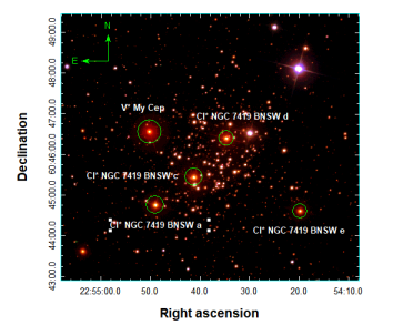
Figure 1: RGB color image of NGC 7419 using observations by filters $g$, $r$ and $i$ of the SDSS telescope for an area of 7 arcmin x 6 arcmin. The 5 Red Supergiants of this cluster are marked with green circles.

In this paper, we focus on the young cluster, NGC 7419 (fig. 1), located at a distance of $\sim$ 2.9 – 4 kpc (Marco & Negueruela 2013; Subramaniam et al. 2006; Beauchamp et al. 1994) with previously reported ages ranging from 14-15 Myr (Marco & Negueruela 2013; Beauchamp et al. 1994) to 22-25 Myr (Subramaniam et al. 2006; Joshi et al. 2008). These studies also show that NGC 7419 is rich in CBe stars. Marco & Negueruela (2013) shows that NGC7419 has a very high fraction ($\sim$ 40 $\%$) of Be stars among the early B type stars, whereas very few Be type stars at later spectral class. They also report strong variability in the emission characteristics of Be-type stars in the cluster. The abundance of CBe stars in the cluster suggests that there should be some mechanism at work by which a large fraction of the early B-type stars possess high rotational velocity (Subramaniam et al., 2006). NGC 7419 also has 5 notable Red Supergiants, with no blue supergiants, the highest in any cluster till the end of the 20th century. The Red Supergiants in the cluster are i) Cl* NGC 7419 BNSW d, ii) V* MY Cep, iii)Cl* NGC 7419 BNSW c, iv) Cl* NGC 7419 BNSW a, v) Cl* NGC 7419 BNSW e, with V* My Cep being the most luminous Red Supergiant.

Though NGC 7419 has a large number of CBe stars and 5 Red Supergiants, a detailed membership analysis of the cluster and the characterization of its CBe stars are still missing. In this paper, we perform the membership analysis of cluster NGC 7419 using GAIA DR3 data and also perform a variability analysis of the bright members of the cluster in optical and IR wavelengths. One of the goals of this work is to analyze the properties of the CBe-type stars, search for variability, and possibly classify them into periodic and non-periodic variables. Also, Red Supergiants often show slow, irregular variability with no detectable periodicity (Kiss et al., 2006), and in this paper, we analyze the variability of Red Supergiants of the cluster given their lightcurves satisfy certain quality criteria.

The paper is organized as follows. Section 2 deals with various data sets used for the analysis, Section 3 describes the membership analysis, and Section 4 is on finding possible CBe candidates based on sources that show $H\alpha$ excess. Sections 5 and 6 the variability analysis of the candidate members in the cluster using optical and infrared time series data. Section 7 discusses the correlation between WISE CMDs and global trends in Be star’s disk activity, spectral type, and variability, and the observation of different time scales of variability due to different mechanisms seen in CBe stars. Finally, section 8 concludes the results.

2 Data Sets Used

Various archival data sets from the following surveys are used for Membership analysis as well as to search for variable stars within the cluster NGC 7419. Details of individual data set are given below.

2.1 Gaia DR3

Gaia, a European Space Agency observatory launched in 2013, was set to operate until around 2022. It measures star positions, distances, and motions with high precision. The third data release (Gaia DR3) offers five-parameter astrometry and three-band photometry for about 1.5 billion stars, significantly improving upon Gaia DR2 (Gaia Collaboration et al., 2018a) with a 30% increase in parallax precision, double the accuracy for proper motions and reduced systematic errors. The photometry also features increased precision but, above all, much better homogeneity across color, magnitude, and celestial position. A single passband for G, BP, and RP is valid over the entire magnitude and color range, with no systematics above the 1 percent level (Gaia Collaboration et al. 2016, 2023). Vizier (Ochsenbein et al., 2000) was used to obtain the necessary Gaia DR3 data. We obtain Gaia DR3 data to perform the membership analysis and obtain the fundamental parameters of NGC 7419. Given the tidal radius of the cluster reported to be around 5 arcmin (Caron et al., 2003a), we extracted the Gaia DR3 data, which is centered around the coordinates resolved by SIMBAD, i.e., RA = 22:54:18.96; Dec = +60:48:50.4 for a conservative area within 12 arcmin radius along with the following constraints: $0.1mas<\pi<0.8mas$ and non-null values for PMRA (proper motion in right ascension), PMDEC (proper motion in declination), ra (right ascension), dec (declination), Gmag (green), BPmag (blue) and RPmag (red). We consider sources with renormalized unit weight error (RUWE < 1.4, Lindegren et al. 2021) to avoid blended objects. The above parallax range was chosen, which includes the majority of the known members of the cluster (see details below), including the supergiants, as well as to exclude the field contaminants with extreme parallax values. A total of 2913 sources are retrieved within these criteria.

2.2 ZTF (Zwicky Transient Facility) DR18

The Zwicky Transient Facility is a wide-field sky astronomical survey using a new camera attached to the Samuel Oschin Telescope at the Palomar Observatory in California, United States (Masci et al., 2018). It was commissioned in 2018 and is named after the astronomer Fritz Zwicky. With time series observations in $r$, $g$ and $i$ bands, the Zwicky Transient Facility is designed to detect transient objects that rapidly change in brightness, for example supernovae, gamma ray bursts, and collision between two neutron stars, and moving objects like comets and asteroids (Bellm et al., 2018).

For candidate members of NGC 7419, we use the ZTF Data Release 18, released on July, 2023. This release adds two months of observations to the DR17 data release, up to 7 May 2023, for the public portion of the survey and private survey time before 4 Jan 2022. We use the ZTF $r$-band data in the footprint 1837 and 831 within a 12’ radius of NGC7419 as it had the highest number of cross-matches with the candidate members identified from Gaia DR3 (see section 3). The other two bands, $g$ and $i$, had very low average number of observations per lightcurve and hence we do not consider them. We considered the $r$-band data for only those sources which had more than 50 good quality observations (catflags < 32768). Data within 100 days in each lightcurve was considered as one epoch, and only magnitudes in each epoch that fall within the range of median value $\pm$ 2 standard deviations of that epoch were considered. The median cadence for all crossmatched lightcurves was $\approx$ 1 day.

2.3 Wide-field Infrared Survey Explorer (WISE) and NEOWISE Reactivation Database (2023)

We used the mid-IR photometric data obtained by the Wide-field Infrared Survey Explorer (WISE; Wright et al. 2010). WISE was launched in 2009 and performed its cryogenic all-sky survey for about a year in four bands: W1 (3.4 $\mu$m), W2 (4.6 $\mu$m), W3 (12 $\mu$m), and W4 (22 $\mu$m). We use data in the W1 and W2 filters, which have saturation limits of W1 = 8 mag and W2 = 7 mag (Cutri et al., 2012).

NEOWISE utilizes the space telescope Wide-Field Infrared Survey Explorer (WISE). The WISE spacecraft was brought out of hibernation in September 2013 and renamed as NEOWISE with a mission to detect and characterize asteroids and comets, and to learn more about the population of near-Earth objects that could pose an impact which could be hazardous to the Earth. The NEOWISE 2023 Data Release includes the single-exposure images and photometry in 3.4 and 4.6 $\mu m$ (W1 and W2) bands that were acquired between December 13, 2020 and December 13, 2021 UTC, along with data gathered from the previous 8 years (Mainzer et al. 2011, 2014) in multiple epochs. An epoch in NEOWISE data typically spans 180 days, with each epoch containing anywhere from 4-30 observations with a near uniform cadence of 0.066 days.

We considered unsaturated sources with SNR (Signal to Noise Ratio) greater than 3 and having at least 30 good-quality observations. The low value of SNR was opted to obtain multi-epoch photometry for a maximum number of targets as possible.

2.4 The INT Photometric $H\alpha$ Survey of the Northern Galactic Plane (IPHAS)

The INT Photometric $H\alpha$ Survey of the Northern Galactic Plane (IPHAS) is a 1800 square degrees CCD survey of the northern Milky Way spanning the latitude range -5^∘ < b < +5^∘ (Drew et al., 2005). The data in this survey consists of observations in the $H\alpha$ narrow-band along with Sloan r^′ and i^′ broad-band filters. Any source with SNR>5 is included here. This survey has the saturation limits at 13, 12, and 12.5 magnitudes in r^′ , i^′ , and $H\alpha$ bands, respectively (Barentsen et al., 2014).

3 Membership analysis of NGC 7419 using Gaia DR3 and machine learning techniques

The groundbreaking studies by Sanders (1971) and Vasilevskis et al. (1958) utilized proper motion measurements of stars to verify their membership. They employed a bivariate Gaussian mixture model (GMM) to represent the distribution of stars in the vector point diagram (VPD). Subsequently, Kozhurina-Platais et al. (1995) enhanced the membership probability assessments by incorporating the celestial coordinates of the stars along with their proper motions. Then, in recent history, photometric and astrometric measurements, celestial coordinates were used together for unsupervised and supervised algorithms in the works of Sarro et al. 2014; Galli et al. 2020; Breiman 2001; Pedregosa et al. 2018; Das et al. 2023; Gupta et al. 2024, to name a few. We use a combination of an unsupervised learning algorithm, Gaussian mixture model (GMM), and a supervised learning algorithm, Random Forest (RF), in order to identify the membership of the sources within 12’ radius of the cluster using Gaia DR3 data (see Das et al. 2023; Gupta et al. 2024 for details). The steps for the analysis are detailed below.

3.1 Membership using Gaussian Mixture Model

A Gaussian mixture model (GMM) is a probabilistic model that assumes all the data points are generated from a mixture of a finite number of Gaussian distributions with unknown parameters. This algorithm is based on unsupervised learning and is a soft probabilistic clustering, and it gives probabilities of cluster membership instead of just membership. The main difficulty in learning Gaussian mixture models from unlabeled data is that it usually does not know which points came from which cluster (component) (Bishop, 2006). To solve this problem, an iterative statistical model known as expectation maximization is used, which assumes random Gaussians for the data points to get a preliminary clustering and then uses the obtained clustering to form a new Gaussian. This process is repeated iteratively until convergence criteria like "no further change in cluster assignments" are reached (Murphy, 2012).

Caron et al. (2003a) reports a tidal radius of 5 arcmin for NGC 7419. Thus, we used a reasonable set of 1031 sources within a 5 arcmin radius for GMM. Choosing a small radius like this will ensure that the astrometric and photometric properties of the stars in this region should represent the whole complex, and also, at the same time, the field-star contamination would be as minimal as possible. After running GMM analysis, of the 1031 sources, 525 high probability members with the probability being greater than 0.9. This is reasonable as previous works along these lines use probability of 0.8 as their membership cutoff (Das et al. 2023; Gupta et al. 2024). The various features used for this training set were PMRA, PMDEC, parallax, ra and dec.

The Gaussian Mixture Model classified 4 of the 5 supergiants as members. The remaining supergiant (Cl* NGC 7419 BNSW a) was left out probably because it had an anomalously higher PMRA value compared to the other supergiants. We now have a training set consisting of high probability members and non members that can be used in the Random Forest classifier.

3.2 Membership using Random Forest (RF) analysis

Compared to GMM, Random Forest (Breiman, 2001) is a form of Supervised Learning that requires a prior training set (see Das et al. 2023 and Gupta et al. 2024 for details). It uses an ensemble of uncorrelated decision trees for prediction. Since the tree models are not correlated, an ensemble of such uncorrelated tree models will be less biased than a single such model. Each individual tree in the random forest gives a class prediction and the class with the most votes becomes our model’s prediction. These decision trees are trained using the training set and to decrease correlation between trees, random sampling with replacement on the training set is performed. This sampling is performed on data points themselves as well as features for classification.

We use the output from the GMM analysis to create a training set for the RF algorithm. We consider the 2913 sources within a 12 arcmin radius of the cluster as a test set for the RF algorithm and the 5 arcmin data obtained from GMM analysis consisting of high probability members and non-members as the training set.

After running the RF algorithm, 562 sources are classified as members, which satisfies the probability criteria greater than 90%. The algorithm classifies 3 out of the five supergiants in the cluster as members, whereas the remaining two supergiants are manually included in the member list as they are already well-known cluster members from previous studies (Marco & Negueruela 2013; Beauchamp et al. 1994) and had a probability of being cluster members of 0.86 and 0.87 respectively. This takes the number of probable members within a 12 arcmin radius to 564.

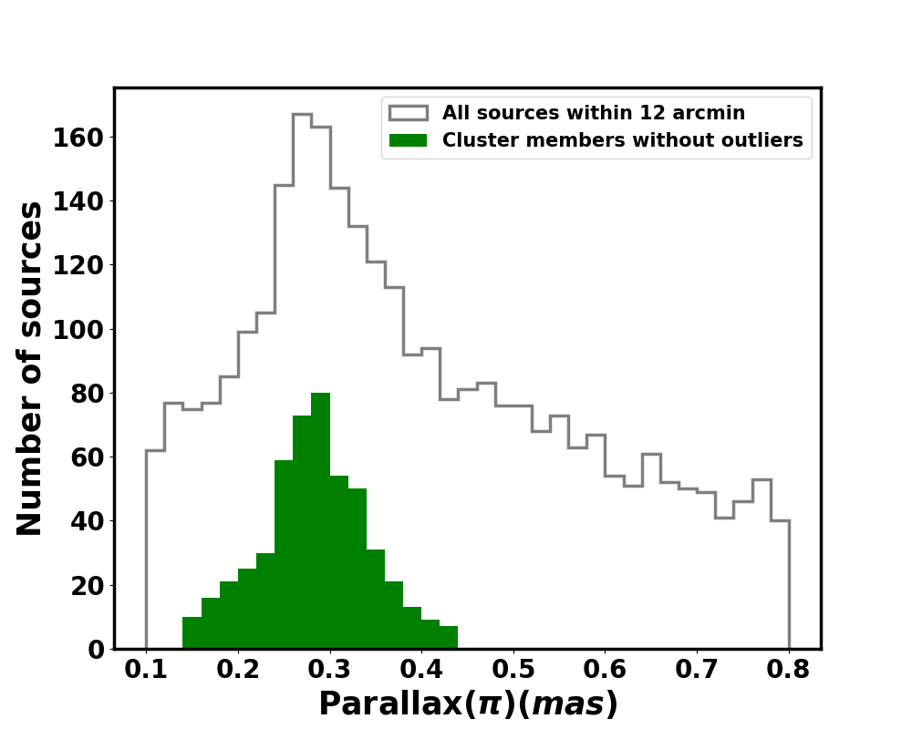
Figure 2: Histogram distribution of parallax of all the sources (grey) within 12 arcmin radius of the cluster NGC 7419 along with the candidate members (green) selected based on the Random Forest classification. See text for details.

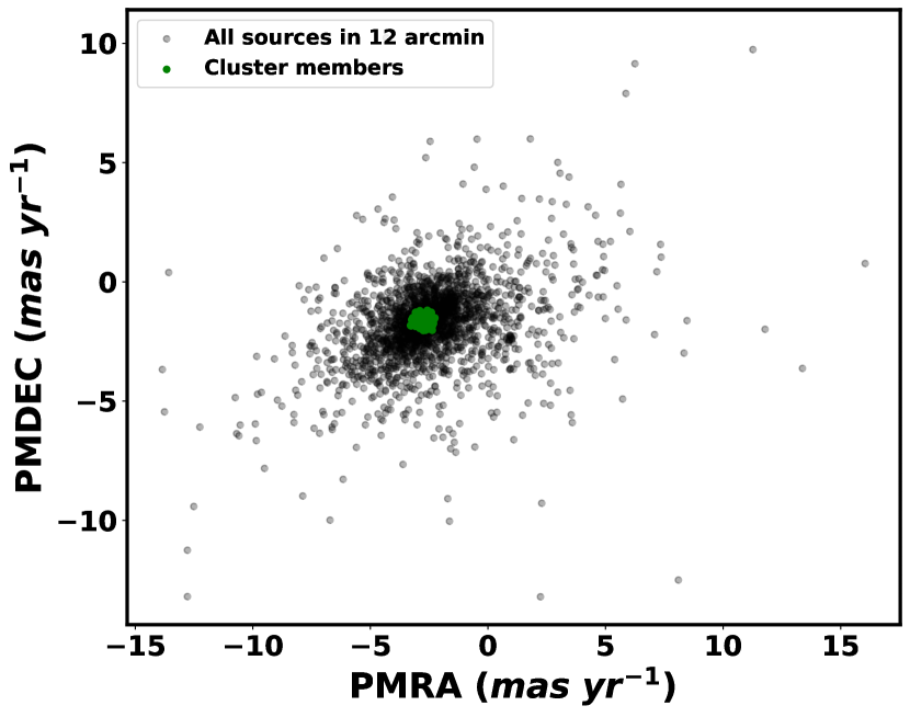
Figure 3: PMRA vs. PMDEC distribution of all the sources within 12 arcmin radius of the cluster (grey dots) along with the probable candidate members selected based on the Random forest classification (green dots).

From RF analysis, the candidate members we identify have a parallax distribution of 0.11 to 0.52 $mas$, which corresponds to a huge range in the distance, from 2000 to 9000 pc), with the majority of them peaking around 3400 pc. In order to further filter out the possible field contaminants, we perform a box-plot analysis and the outliers are removed by considering only sources within 1.5 times the inter-quartile range (IQR) of the median parallax value. The resultant sources has parallaxes within 0.14 - 0.43 $mas$ with a mean value of 0.283 $mas$. After removing the outliers, 499 candidate members remained. Among these members, 70% were present within 5 arcmin of the center (coordinates in section 2.1), and 90% were present within 10 arcmin from the center. The candidate members with their parallax, proper motion, and magnitude information are given in Table 5. They have mean proper motions of -2.73 $\pm$ 0.15 $mas\ yr^{-1}$ and -1.60 $\pm$ 0.15 $mas\ yr^{-1}$ in RA and DEC, respectively.

Figure 2 represents the parallax ($\pi$) distribution of all the sources within 12 arcmin radius of the cluster, along with parallax for the candidate members highlighted in green.

Figure 3 represents the PMRA vs. PMDEC plot for the RF selected candidate members against all the sources within 12 arcmin of the cluster. Both Figures 2 and 3 show that the above algorithms efficiently identify the candidate members of the cluster from a large pool of field stars, which otherwise would have been difficult.

We compare the candidate members identified in the above analysis with the spectroscopically identified membership of the cluster by Marco & Negueruela (2013). They had 141 spectroscopically confirmed B-type members between 5 and 14 $M_{\odot}$. Cross-matching our candidate members with their sample within a match radius of 1 arcsec, we found 127 common sources in both catalogs. Thus, our membership includes 90% of cluster members found in Marco & Negueruela (2013). Figure 4 is a BP-RP vs. G color-magnitude diagram (CMD) of all the Gaia DR3 sources within 12 arcmin radius of the cluster along with the 499 candidate members highlighted in green and the 127 common sources found in Marco & Negueruela (2013) in red. Lastly the supergiants are not present in the 127 common sources since the spectroscopy study had identified only B-type stars. From the CMD in fig. 4, the newly identified cluster members overlap well with previously known sources, and the current analysis is detecting candidate members 2 mag deeper than the previous spectroscopic analysis.

3.3 Distance and age of the cluster

The mean and standard deviation of the parallax of the 499 candidate members identified in section 3 is 0.28 $\pm$ 0.06 $mas$ which corresponds to the mean distance to the cluster as 3.6 $\pm$ 0.7 $kpc$.

Although Gaia provides high-quality photometric data, including parallax, simply inverting the parallax to get the distance leads to biases that tend to get larger for larger parallax uncertainties as well as distant objects (Bailer-Jones et al., 2021b). Hence, a proper statistical treatment is needed to avoid this biasing, the results of which are compiled in the Bailer-Jones Catalogue (Bailer-Jones et al., 2021a). Geometric distances are computed using direction-dependent priors while, photogeometric distances are computed using colors and apparent magnitude. We also estimate the distance to the cluster using this catalog to compare it with the above-estimated distance. In the Bailer-Jones Catalogue, we prefer photogeometric distance over geometric distance as NGC 7419 is quite a distant cluster, which implies higher uncertainties associated with parallax data as described in Bailer-Jones et al. (2021a). After removing the outliers, we estimate the distance to the cluster using this catalog to be 3.3 $\pm$ 0.6 $kpc$, which agrees with the above measurement, within uncertainty.

Subramaniam et al. (2006) and Marco & Negueruela (2013) estimated average distances of 2.9 $kpc$ and 4 $kpc$, respectively for the cluster. Both these studies used zero-age main sequence fit to the CMD to get the distance after accounting for the reddening towards the cluster. Since the distance estimated from the mean parallax method is in agreement with the Bailer-Jones et al. (2021a) catalog, hereafter we consider our calculated distance to the cluster as the cluster distance which is 3.6 $\pm$ 0.7 $kpc$.

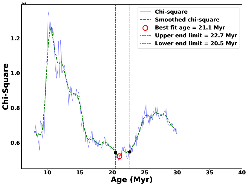
Figure 15: Chi-square values for isochrones of ages in the range of 8-30 Myr for NGC 7419. The red open circle indicates the lowest chi-square value (best fit) corresponding to the 21.1 Myr isochrone. The green dashed vertical lines indicate the upper and lower limits within 5% of this age.

In order to obtain the average age of the cluster, we obtain isochrones of several ages from 8 to 30 Myr (based on previous literature) from PARSEC models (Bressan et al., 2012) and correct them for the cluster distance of 3.6 $kpc$ and extinction, $A_{V}$. We take the extinction, $A_{v}$ towards the cluster to be 5.2 mag from previous literature (Bhatt et al., 1993; Subramaniam et al., 2006; Marco & Negueruela, 2013) and correct each isochrone using equation 1 and the extinction coefficients provided in Gaia Collaboration et al. (2018b). We interpolate the data points in the isochrone. We then did a chi-square calculation (see fig. 15 in Appendix) using the interpolated magnitudes and observed magnitudes in the following way:

$$\chi^{2}=\sum_{i=1}^{N}\frac{(O_{i}-E_{i})^{2}}{\sigma_{i}}\,,$$ (1)

where $O_{i}$’s are the observed magnitudes and $E_{i}$’s are the interpolated isochrone magnitudes, and $\sigma_{i}$’s are the corresponding uncertainties in the observed magnitudes.

We find the best average age of the cluster, which comes out to be around $21.1^{+1.6}_{-0.6}$ Myr, corresponding to the minimum chi-square value. We determine the uncertainty by taking the upper and lower bounds within 5% of the best-fit age. The isochrone of 21.1 Myr fits well with the five supergiants lying towards the upper right of the CMD as well as the main sequence distribution of the members, which is evident in Fig 4. Since Gaia G band magnitudes have a lower limit of around 20 mags (Gaia Collaboration et al. 2023; Marton et al. 2023), we can find members with masses above $\sim$1.2 M$\odot$ (for an age of 21.1 Myr, $A_{V}$ of 5.2 mags, a distance of 3.6 kpcs, PARSEC models). Our estimated age is comparable to those reported in previous literature (Joshi et al. 2008; Subramaniam et al. 2006). Using the stellar mass information from the best fit PARSEC isochrone and comparing it with the modified table from Pecaut & Mamajek (2013) to estimate the mass and spectral type of the main sequence stars in this cluster which do not have previous spectral classification. Combining our estimates with previously known spectral types of members (Caron et al. 2003b; Subramaniam et al. 2006; Mathew & Subramaniam 2011; Marco & Negueruela 2013), we find that 75% of these stars are B type with masses ranging from $1.2\ \mathrm{to}\ 12.6\ M\odot$. Since the cluster is relatively evolved and distant, and because of the limited sensitivity of the GAIA data, we do not trace most of the pre-main sequence branches in the CMD.

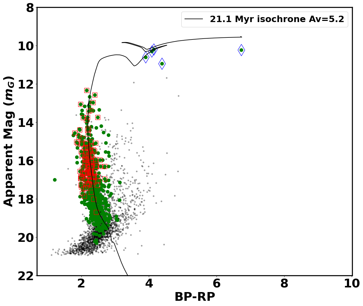
Figure 4: BP-RP versus G-band Color-magnitude diagram for all the sources within 12^′ radius of the cluster NGC 7419 (grey dots). Green dots represent the candidate members selected based on the GMM and RF analysis after removing the outliers. Open red squares are the common sources between this analysis and the spectroscopic member list from Marco & Negueruela (2013). Open blue diamonds indicate Red Supergiants within the cluster. The solid curve represents the 21.1 Myr isochrone from PARSEC models (Bressan et al., 2012) after correcting for the distance and extinction $A_{V}$ = 5.2 mag.

4 Search for $H\alpha$ emission line sources

We use the IPHAS photometry in r^′, i^′, and $H\alpha$ bands to identify the candidate emission line sources within NGC 7419 (Barentsen et al. 2011; Dutta et al. 2015). Of the 499 candidate cluster members, 490 common sources are obtained in the IPHAS catalog. We follow the method described in Barentsen et al. (2011) to identify the $H\alpha$ sources. Fig. 5 shows the r^′-i^′ vs. r^′-$H\alpha$ color-color diagram for candidate members of NGC 7419. The synthetic main sequence tracks given in Drew et al. (2005) for E(B-V)=0, corrected for the cluster reddening $A_{V}$= 5.2 mag using the extinction relations given in Barentsen et al. (2011), are shown as a dotted curve in fig. 5. Those sources lying above 5 sigma threshold from the main sequence are considered to be $H\alpha$ excess or emission line sources where $\sigma$ was determined from the photometric uncertainty in the following way (Barentsen et al. (2011)):

$$(r^{\prime}-H\alpha)_{star}-(r^{\prime}-H\alpha)_{threshold}>5\sigma\,,$$ (2)

where,

$$\sigma=\sqrt{\sigma^{2}_{(r^{\prime}-H\alpha)}+m^{2}\sigma^{2}_{(r^{\prime}-i^{\prime})}}\,,$$ (3)

and $m$ is the local slope of the threshold. We find a total of 42 sources to satisfy this criterion, of which 30 are already known CBe stars from previous spectroscopic studies (Caron et al. 2003b; Subramaniam et al. 2006; Mathew & Subramaniam 2011; Marco & Negueruela 2013). Hereafter, we update the list of candidate CBe members of NGC 7419 with these 42 sources and the previously known CBe members from the literature. We also see that using a method similar to Navarete et al. (2024) for identifying sources showing $H\alpha$ excess results in nearly identical numbers. This brings the total number of unique candidate CBe members in NGC 7419 up to 49 out of which we classify 46 as members in section 3. We use these 49 CBe stars in the later sections as the list of CBe stars in the cluster. Given the cluster’s age ($\sim$ 21 Myr), these stars cannot be Herbig AeBe types, which typically are of age $\sim$ 1-2 Myr (Manoj et al., 2006). From previous studies (Caron et al. 2003b; Subramaniam et al. 2006; Mathew & Subramaniam 2011; Marco & Negueruela 2013) and our earlier spectral type estimation in section 3.3, we find 85% of CBe stars to be early-type (B0.5V-B3V), 9% (B4V-B6V) to be mid-type, and 6% (B7V-B9V) to be late-type. The fraction of CBe to (B+CBe) members comes out to be 46/376 or 12.2%.

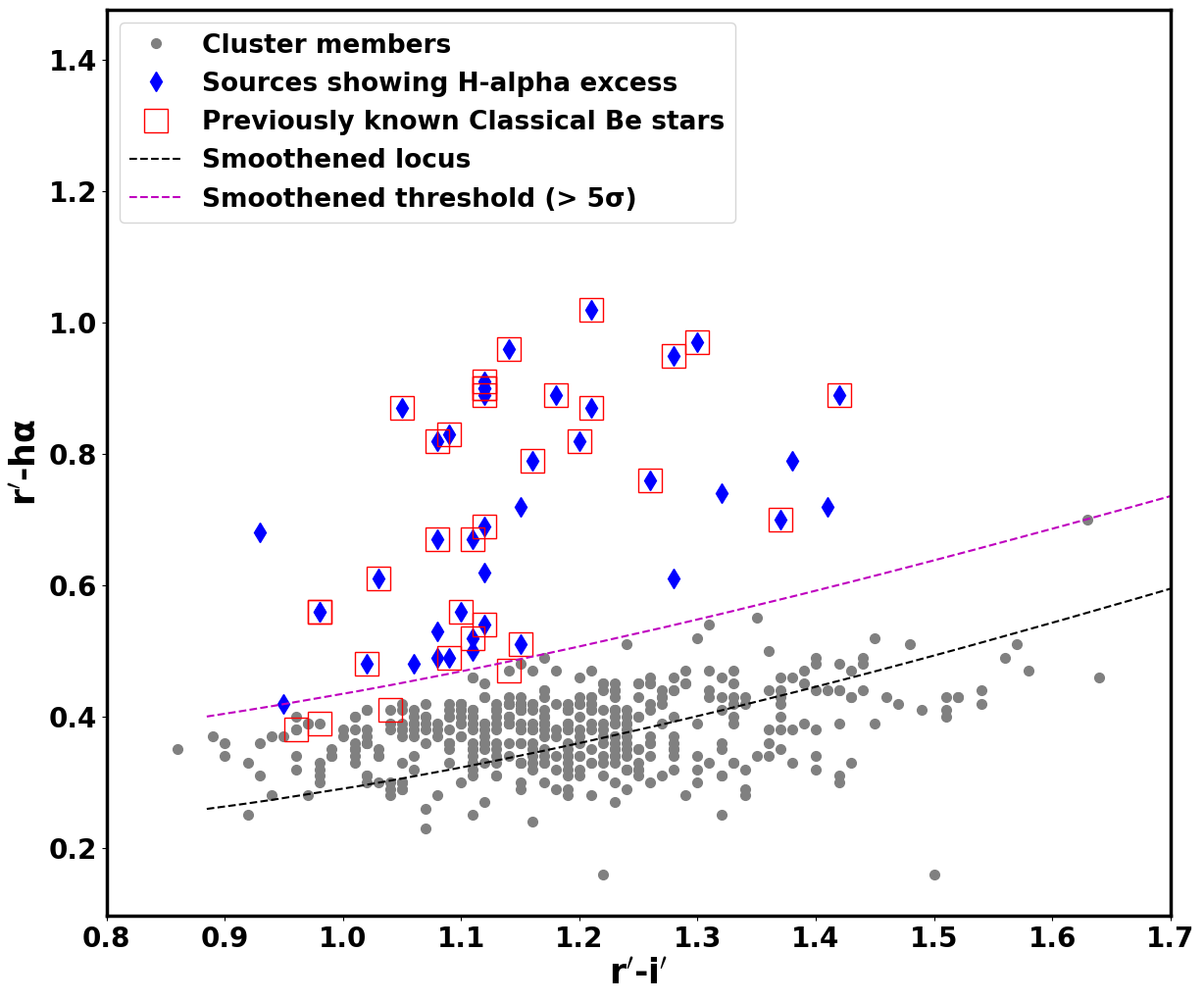
Figure 5: IPHAS color-color diagram with main sequence locus (black curve) and 5 sigma threshold (purple curve) showing sources (blue diamonds) with $H\alpha$ excess. The previously known CBe stars are marked in red boxes.

5 Identification of variable sources using ZTF data

We obtain 476 crossmatches out of 499 from the ZTF survey in the $r$ band in the field with footprints 1837 and 831. We did not use any other bands as sufficient data points are not available. For the $r$-band, only sources with 50 or more good-quality observations are considered. Among these 476 crossmatches, duplicate lightcurves for the same source position are present, and hence we choose the field with the greatest number of observations. Fig. 6 shows the distribution of mean uncertainty in ZTF lightcurves as a function of mean magnitude for all the above sources. It is clear that photometric uncertainty becomes exponentially high ($>$ 0.04 mag) for sources fainter than 18 mag in the $r$-band. The magnitude here is the average magnitude through all available epochs. Hence only those sources with less than 18 mag are considered further for the variability analysis. All of this combined reduced the number of sources for variability analysis using ZTF data to 288. We filter the individual lightcurves to include only data within 2 standard deviations of the median in each epoch group (100 days for ZTF). This choice of 100 days is motivated by the fact that we primarily want to investigate the periodicity of CBe star variability in the short term (from stellar pulsation on timescales of a few hours to days or disk formation or dissipation and wave motions in the decretion disk on timescales of a few months). This evidently excludes very long-period periodicity, which is also observed in CBe stars due to disk growth or dissipation (Rivinius et al., 2013) and will be investigated in a future paper. We find 44 CBe counterparts after crossmatching these 288 sources with the updated CBe star list.

Following this, we use three different methods for our variability analysis: Standard Deviation, Median Absolute Deviation, and Stetson Index (Stetson (1996)).

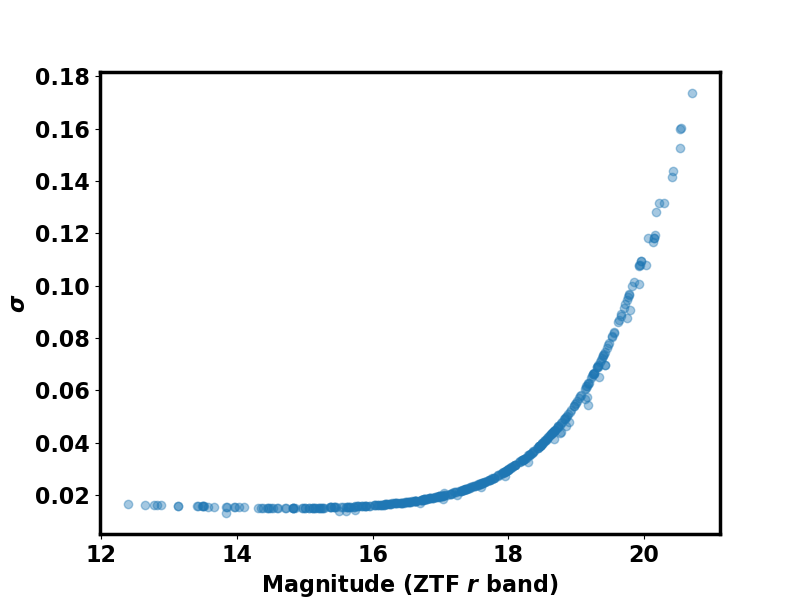
Figure 6: Mean Magnitude vs. Mean error($\sigma$) in magnitude for sources retrieved from ZTF $r$-band observations.

5.1 Variability from Standard Deviation and Median Absolute Deviation

Standard deviation and Median absolute deviation(MAD) are fairly common methods for identifying variability (Sokolovsky et al., 2016a). Standard Deviation and Median absolute deviation are defined below, respectively:

$$Standard\ Deviation(\sigma)=\sqrt{\frac{\sum_{i=1}^{n}(m_{i}-\overline{m})^{2}}{n-1}}\,,$$ (4)

$$MAD=median(abs(m_{i}-median(m))\,,$$ (5)

where $m_{i}$ is the i^th magnitude of a given lightcurve.

The Standard Deviations (Std) and Median absolute deviations (MAD) are plotted against the respective Mean Magnitudes of the 288 ZTF counterparts in fig. 7. A main locus has been traced using a least squares fit, which uses the median ($\sigma$) Std and MAD values of the sources instead of the mean so as not to be affected by outliers. The 3$\sigma$ threshold is shown in Fig. 7. Any source lying above the 3$\sigma$ line has been considered as a variable. Thus 113 probable variables are obtained from the standard deviation method, and 105 probable variables are obtained from the MAD method, with 99 crossmatches between the two methods.

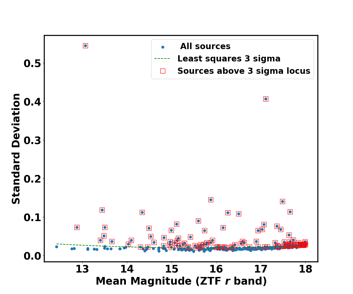
(a) Standard Deviation

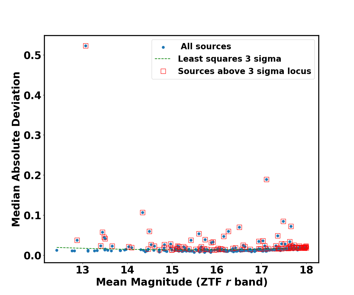
(b) MAD

Figure 7: Standard Deviation and MAD of sources in ZTF data as a function of $r$ band magnitude, along with 3$\sigma$ locus.

5.2 Variability from Stetson Index

The robust version of the Stetson Index (Stetson 1996; Cody et al. 2014) has been computed for the sources with ZTF $r$-band data. It uses quasi-simultaneous 2-band data to determine the correlation between them. The expression for Stetson Index (J) is given by

$$\textrm{J}=\sum_{i=1}^{n}\mathrm{sgn}(P_{i})\sqrt{|P_{i}|}\,,$$ (6)

where,

$$P_{i}={\frac{n}{n-1}}(\delta b_{i}\cdot\delta v_{i})\,,$$ (7)

where $n$ is the number of observations in the lightcurve, sgn is the signum function that gives the sign for the corresponding values of $P_{i}$, $b_{i}$ and, $v_{i}$ are the two band magnitudes at a given epoch and $\sigma_{b_{i}}$ and $\sigma_{v_{i}}$ are the defined as the respective uncertainties.

$$\delta b_{i}=\frac{b_{i}-\overline{b}}{\sigma_{b_{i}}}\,,\delta v_{i}=\frac{v_{i}-\overline{v}}{\sigma_{v_{i}}}\,,$$ (8)

Here, $\delta_{b}$ and $\delta_{v}$ are called the residuals. For a nonvariable star, the photometric errors, $\sigma_{b}$ and, $\sigma_{v}$ are random, and hence the residuals, $\delta_{b}$ and $\delta_{v}$ are uncorrelated, and for large $n$, their Stetson Index tends to zero.

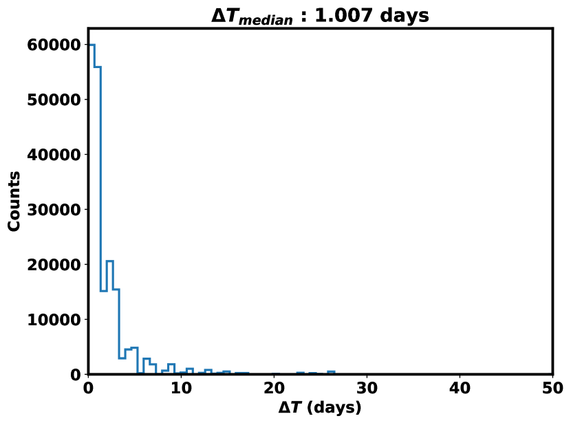
Figure 16: Histogram of $\Delta$T values for ZTF lightcurves. $\Delta$T is the time difference between two consecutive observations in a lightcurve.

For variables, the residuals, $\delta_{b}$ and $\delta_{v}$ are correlated since the phenomenon that governs the variation will change the brightness in the same direction for both the bands, and so the Stetson Index for variables will be some positive constant. This method is useful only for cases where the time between successive observations is small compared to the variation period (Welch & Stetson, 1993). The ZTF data we consider here is only for a single band, whereas the computation of the Stetson Index requires two-band data. To overcome this, a method similar to that described in Sokolovsky et al. (2016b) is adopted. We chose a $\Delta T_{max}$=1 day between corresponding observations of the odd and even lightcurves (see Sokolovsky et al. 2016b for details) for deciding which data points will be considered for Stetson Index computation. This cutoff is chosen after analyzing a histogram of $\Delta T$ (see fig. 16 in Appendix) for all ZTF lightcurves for our cluster. The single-band data is split into two by taking the odd indexed data points as one band and the even indexed data points as the second. A heuristic cutoff is chosen based on the median value ($\sigma$) of the index and accepting any source with J value greater than 3$\sigma$ to be a candidate variable.

From the computation of the Stetson Index for 288 sources, those with the Stetson Index greater than 3 times the median value (J > 146) for all sources are considered as variables. We choose the median value instead of the mean so as not to let our analysis be affected by outliers. Using this method, 34 sources are classified as variables. Based on the Stetson Index value, we subdivide the 34 variables into 3 categories: Strong, Moderate and Low with the corresponding cutoffs being J > 5$\sigma$, J $\in$ (4$\sigma$, 5$\sigma$] and J $\in$ (3$\sigma$, 4$\sigma$] respectively, where $\sigma$ refers to the median Stetson Index value. In fig. 8, the distribution of the Stetson Index as a function of r-band magnitude is shown, where most sources have a J value around 0 corresponding to non-variables. We identify 34 variable sources which have Stetson Index values in the range of 149.7 to 3261 and are marked in different colors.

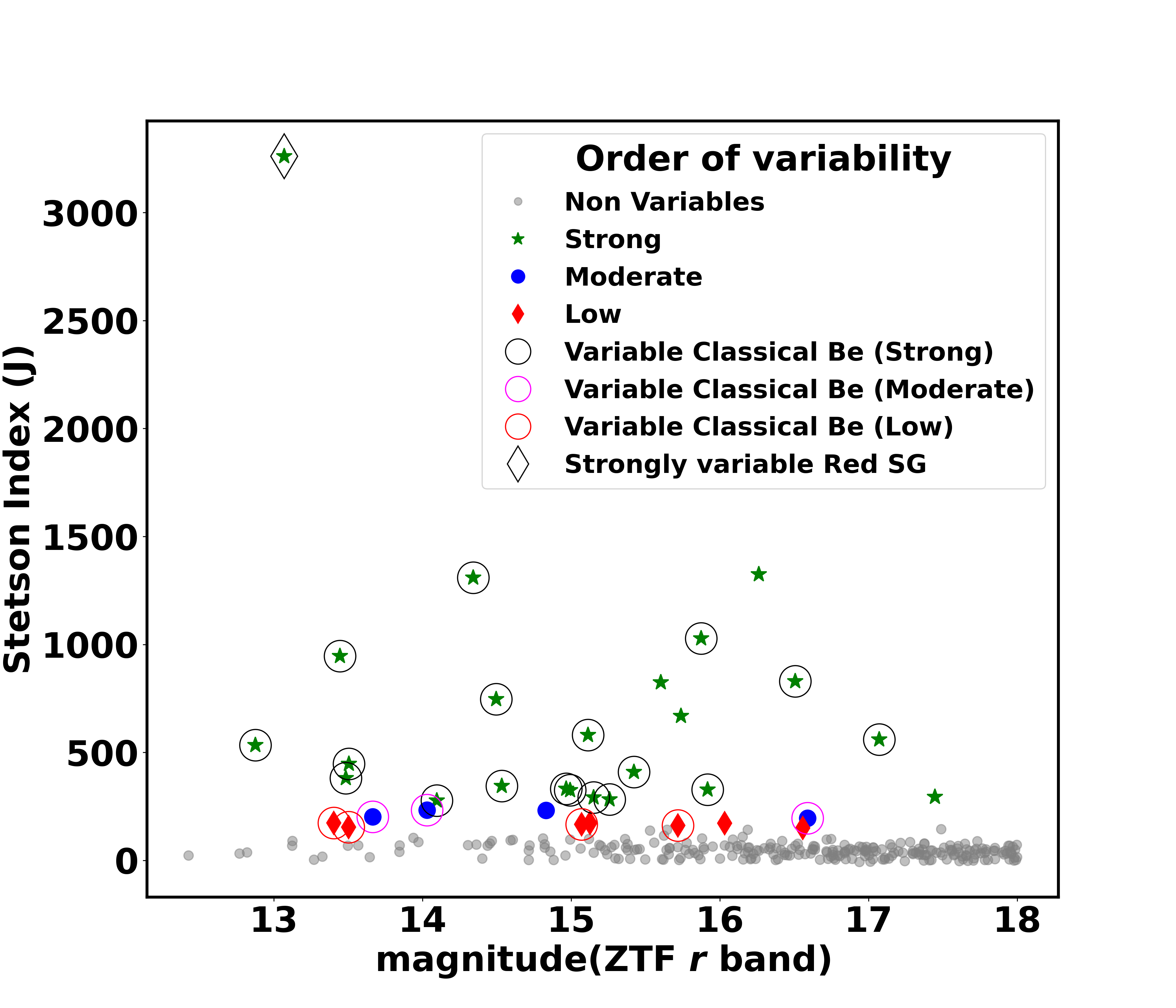
Figure 8: Distribution of Stetson Index (J) as a function of Magnitude (ZTF $r$ band). J represents the order/strength of variability as a function of $r$-band magnitude for the ZTF data. Stars with J greater than 3 times the median Stetson Index value are classified as variables. Different colors represent the order of their variability, which are listed as legends.

A total of 33 sources are variable across all three methods. Hence, from here onwards, we have these 33 sources as the final list of candidate variables in optical, which forms the most reliable list of variables based on 3 different methods.

Cross-matching the 33 variables we identify from ZTF data with the 49 CBe stars in the region, we find 24 CBe stars to be common. Thus almost 50$\%$ of the CBe type stars in NGC 7419 are showing variability in optical wavelength. One out of the five Red Supergiants (V* My Cep) in the cluster is also been present in the list of these variables with a Stetson Index (J) value of 3261 and is highlighted in fig. 8.

5.3 Periodicity Analysis of ZTF light curves using Lomb Scargle Periodograms

We further perform periodic and non-periodic classification using the Generalised Lomb Scargle Peridogram (GLSP), which is a robust version of the original (Scargle 1982; Lomb 1976; Scargle 1982; VanderPlas 2018; Zechmeister & Kürster 2009) on the 288 ZTF sources. The periodogram obtained for each source often contains aliased signals whose frequencies depend on the cadence of the window function (VanderPlas, 2018). The window function is just the resulting power spectrum from running the Lomb Scargle periodogram for a series of measurements that are all equal to unity over the entire duration of the observing window. Using a masking method similar to that described in Kramer et al. (2023) and Ansdell et al. (2017a), we compute periodograms, phase lightcurves and best period of the sources for a period range of 0.025 to 150 days. The lower bound for this period range is taken from Chen et al. (2020) since ZTF lightcurves are unevenly sampled (fig. 16), and thus, using the Nyquist frequency limit (which may or may not exist for an unevenly sampled data) is not feasible (VanderPlas, 2018). The upper bound is chosen due to computational constraints. However, it still incorporates the typical timescales of the variability of CBe stars, which are objects of primary focus for our work due to pulsation/rotation, alternating disk growth and decay, binarity, and wave motions in the disk, leaving out very long-term variations caused by the formation and dissipation of disks (Rivinius et al., 2013) which we discuss in section 7.1. This type of variation is often visible in the raw lightcurve as bursts or drops (Rivinius et al., 2013). For the frequency grid step width, we choose a reasonable value of $n=10$ (VanderPlas, 2018). The overall algorithm is summarized below:

1. Compute window and observed power spectrum from cleaned lightcurves.

2. To get Window peaks, those peaks with Lomb Scargle power above 5$\sigma$ ($\sigma$ = Standard Deviation) of the baseline are considered, which is zero.

3. In order to get observed power spectrum (OPS) peaks, we use argrelmax function from scipy (Virtanen et al., 2020) to get local maxima (significant peaks) with the order parameter set to 1000. We choose the minimum height of each such peak to be greater than or equal to 15% of the maximum peak in the OPS.

4. Using the window function, we remove significant window peaks within 5% of the peaks in the OPS.

5. We then ensure that the remaining peaks are above the False alarm probability threshold of 0.005. False alarm probability denotes peaks that are caused purely by the coincidental alignment of random errors (VanderPlas 2018; Baluev 2008).

6. Finally, we classify a source as periodic if the least squares sinusoid fit has an amplitude higher than the Standard Deviation of the magnitude of that source. Any source that fails to satisfy these criteria is classified as a Non-Periodic or Uncertain.

It should be noted that masking the window aliases may also cause true peaks to get masked if they happen to lie within 5% of the aliases. However, it is still better than naively taking the highest peak as the correct one, as emphasized in VanderPlas (2018) and Kramer et al. (2023). The latter also confirms that only 1-2% of objects are affected by this issue. An example of the result using the above algorithm is shown in fig. 9. It clearly shows that the highest peak is not always the correct one. The highest peak is at around 1 day, but it and its higher frequency aliases are clearly an imprint of the window function on the observed power spectrum and are hence masked out.

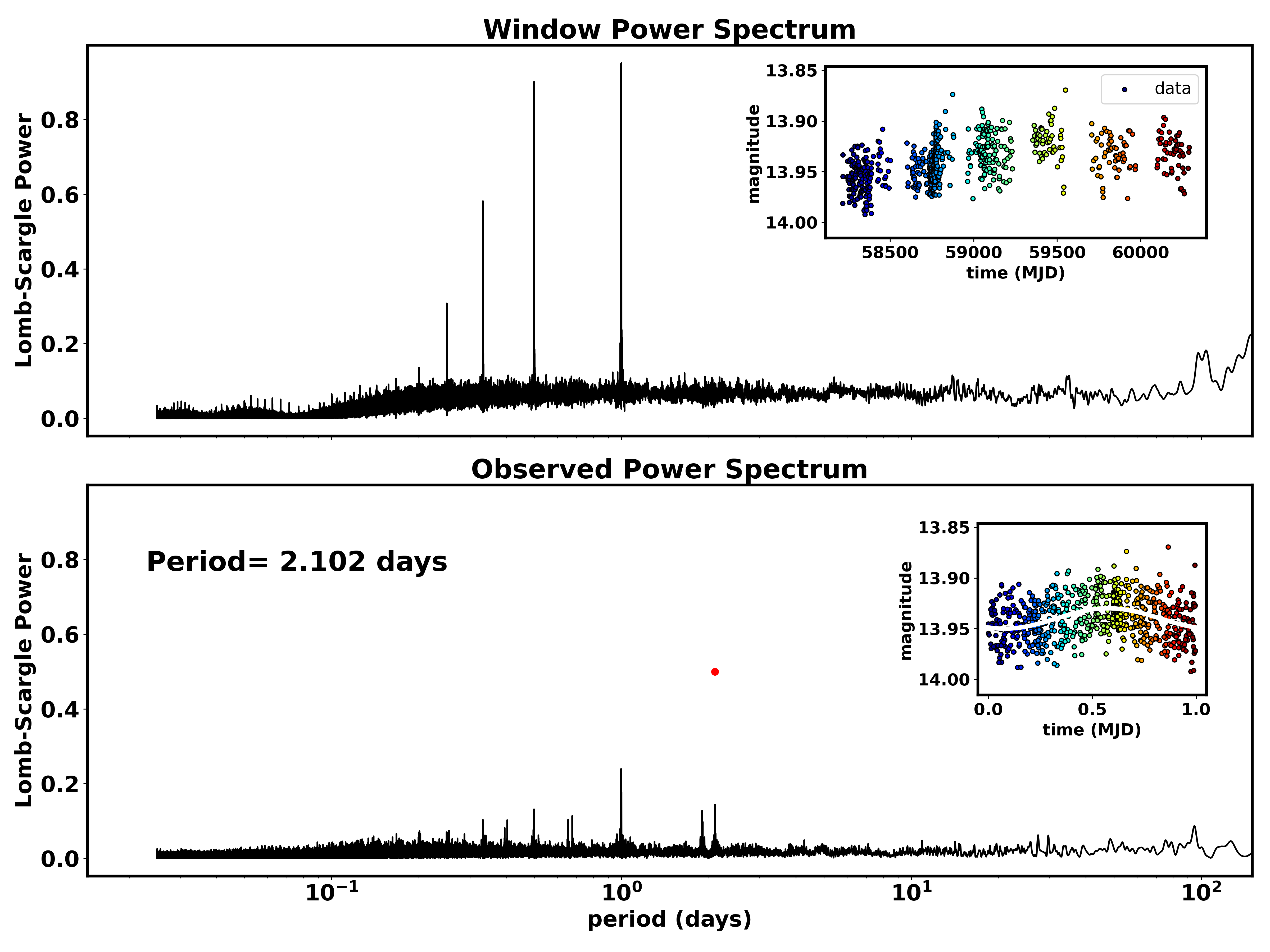
Figure 9: An example output for a periodic star from ZTF data for NGC 7419. The top panel denotes the window power spectrum and the bottom panel denotes the observed power spectrum. Inset plots show the data and the phased lightcurve with the best-fit sinusoid, respectively. The red dot indicates the peak corresponding to the best period.

After removing the window aliases and performing a visual inspection to check for good fitting to the lightcurves, out of 288 ZTF sources, 27 show periodic signals. Out of the 33 variables in optical bands we identify within NGC 7419 (see section 5), we find 12 to be periodic. More than 50% of the periodic sources are non-variables in our work. Looking into it further shows that 14 out of these 15 sources have a positive Stetson Index value, and 6 have a Stetson Index value greater than the median Stetson Index value of all ZTF sources. A positive Stetson Index indicates some correlation in the variation of magnitudes between the two pseudo bands (see section 5.2), which suggests these sources are low amplitude variables that were not identified previously based on our stringent cutoff for high confidence variables. Hence, we define these stars as sub-threshold periodic stars. Out of 44 CBe sources in ZTF data, 10 are classified as periodic. 9 out of these 10 sources are also included in the list of variables. A deeper look into the multiple periodicity, which is common in CBe stars, is discussed in section 7.1. The relative ratio of periodic sources with respect to their total counterparts is shown in fig. 10.

Table 2 represents a summary of the variability analysis using ZTF data. A detailed table for all the ZTF sources showing the results of variability and Periodicity analysis can be found in the Appendix (Table 6).

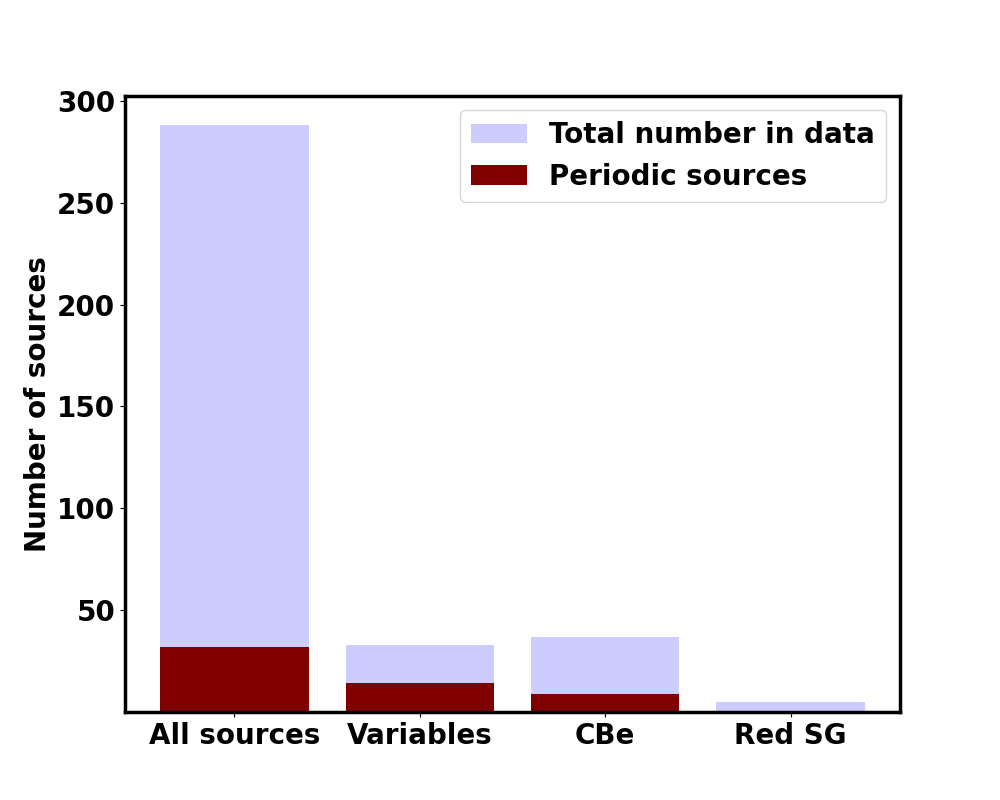
Figure 10: Bar plot showing the relative number of periodic sources for all sources, variables, CBe stars, and Red Supergiants in ZTF data.

Type	NGC 7419	ZTF	NEOWISE
Members	499	288	149
Classical Be stars	49	44	28
Red Supergiants	5	1	0

Table 1: Statistics of NGC 7419 members and their respective crossmatches in ZTF and NEOWISE data

Criteria	Subtype	Count (Non CBe | CBe | Red SG)
	Strong	4 | 18 | 1
Stetson Index (J)	Moderate	1 | 3 | 0
	Low	3 | 3 | 0
	Periodic	17| 10 | 0
Periodic Signal (Lomb Scargle, LS)
	Non Periodic/ Uncertain	222 | 34 | 5

Table 2: ZTF variability summary

6 Identification of variable sources using NEOWISE data

We obtain a total of 302 sources from the NEOWISE survey having time-series photometry in two bands, i.e., in W1 and W2 (3.4 $\mu$m and 4.6 $\mu$m). After considering sources with SNR greater than 3 and having at least 30 good quality observations, and after removing the saturated Red Supergiant (Cl* NGC 7419 BNSW e), we obtain 149 NEOWISE counterparts for NGC 7419. 28 CBe counterparts are included in these 149 sources. All 28 of these CBe sources are also present in the ZTF data. Below we describe the various steps to identify the variable sources in the list. Table 1 summarizes the statistics of NGC 7419 members and their respective crossmatches (satisfying all quality criteria) in ZTF and NEOWISE data.

6.1 Variability from Standard Deviation and Median Absolute Deviation

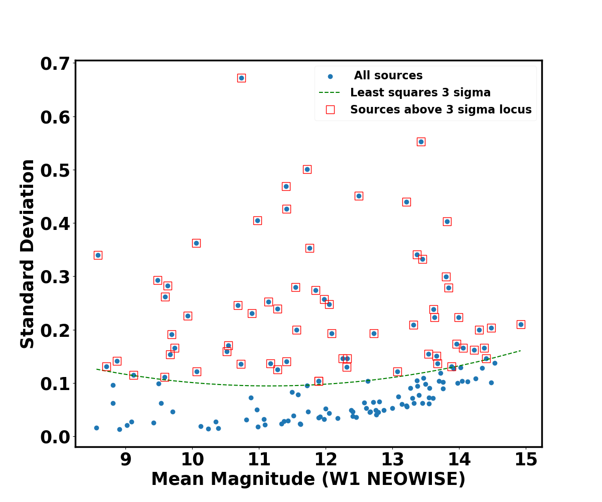
(a) Standard Deviation (W1)

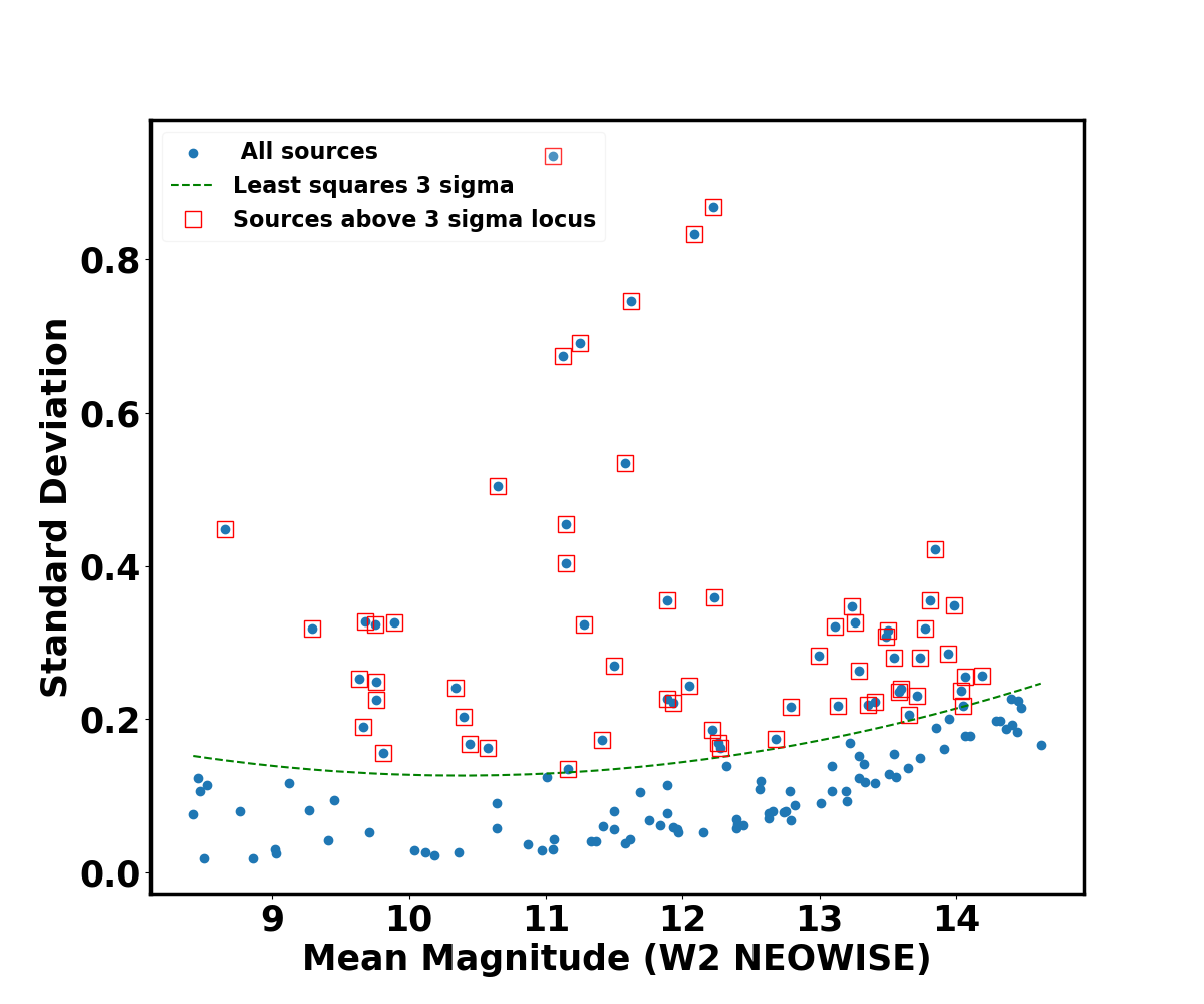
(b) Standard Deviation (W2)

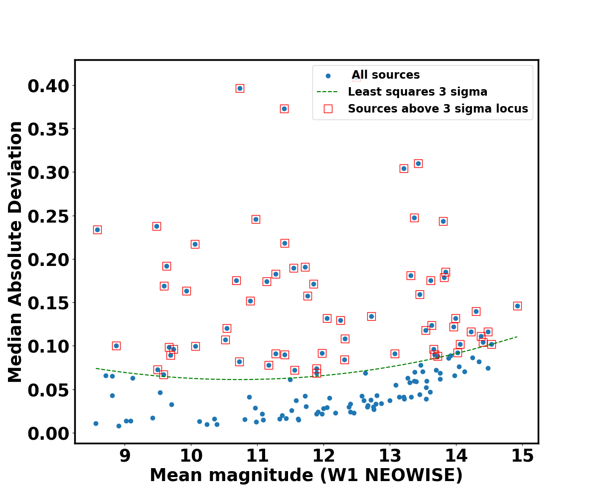
(c) MAD (W1)

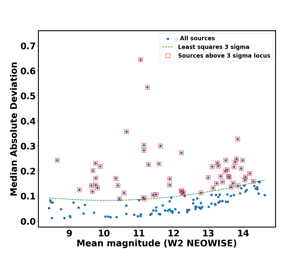
(d) MAD (W2)

Figure 18: Standard Deviation and MAD of sources in NEOWISE data as a function of W1 and W2 band magnitude, along with 3$\sigma$ locus.

Similar to the work done for ZTF data, we consider any source lying above the 3-sigma line a variable. For NEOWISE data, specifically, we perform this for both W1 and W2 bands and take the common sources that satisfy the variability criteria across the two bands as variables. For brevity, these plots are shown in fig. 18 in Appendix(A).

From the standard deviation method, we obtain a total of 54 probable variables and a total of 53 probable variables from the MAD method, with 51 crossmatches between the two methods.

6.2 Variability from Stetson Index

For the Stetson Index computation, unlike the ZTF data, we did not apply the treatment described in Sokolovsky et al. (2016b) as the NEOWISE data include simultaneous 2-band observations. Sources with Stetson Index (J) greater than 3 times the median J value (i.e., J $>$ 180) are considered variable. This led us to identify 36 candidate variables. Similar to the treatment for the ZTF survey (see section 5.2), based on the Stetson Index value, we subdivide the 36 candidate variables into three categories: Strong, Moderate, and Low. The distribution of the Stetson Index as a function of W1-magnitude is shown in fig. 11. Unlike the optical wavelength (see fig. 8), most of the variables we identify in the IR wavelength lie towards the brighter end (W1 $<$ 12.5 mag) compared to the non-variables, which are mostly of W1 $>$ 12 mag. Out of these 36 sources, there are 21 and 20 crossmatches, respectively, with the Standard Deviation and MAD methods, and 20 crossmatches across all three. Hence, from here onwards, like before, we consider these 20 sources as the final list of candidate variables from NEOWISE analysis.

Cross-matching the 20 variables we identify from NEOWISE data with the 49 CBe stars in the region, we find 12 of them to be Be-type stars. Thus almost 25% of the CBe type stars in NGC 7419 are showing variability in NIR wavelength. A total of 7 CBe sources are classified as variable in both optical (ZTF) and NIR (NEOWISE) wavelengths.

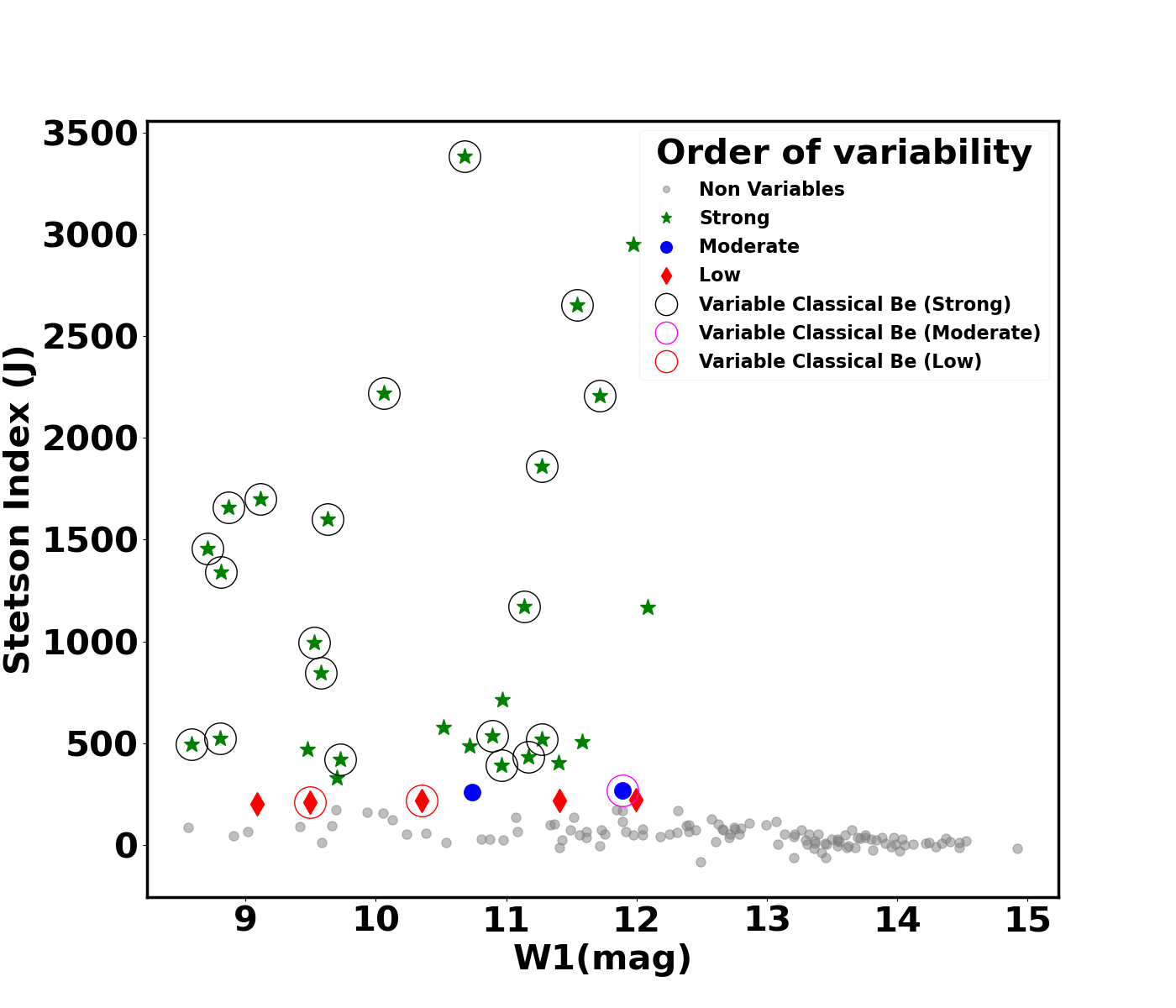
Figure 11: Stetson Index (J), as a function of W1-band magnitude for the NEOWISE data. Stars with J greater than 3 times the median Stetson Index value are classified as variables. Different colors represent the order of their variability, which are listed in the index.

6.3 Periodicity Analysis of NEOWISE light curves using Lomb Scargle Periodograms

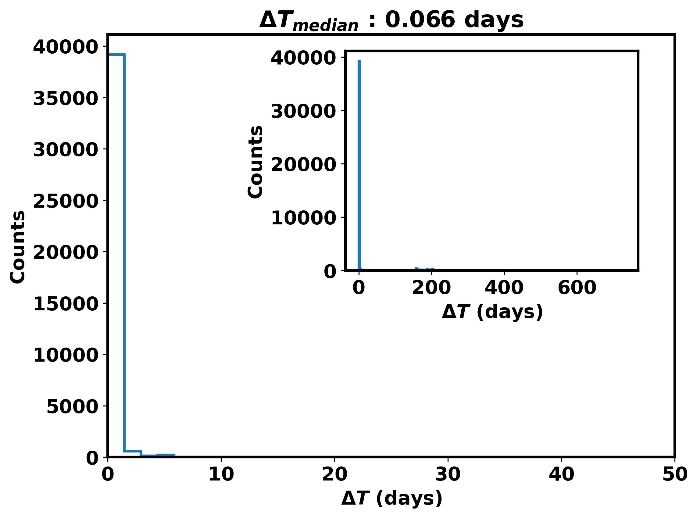
Figure 17: Histogram of $\Delta$T values for NEOWISE lightcurves. $\Delta$T is the time difference between two consecutive observations in a lightcurve.

Using a prescription similar to that in section 5.3, we perform the periodicity analysis of cluster members using NEOWISE data. NEOWISE, being a space-based telescope, has a near-uniform cadence of about 0.066 days (see fig. 17). The slight non-uniformity present is due to the SNR limit that we enforced when gathering the light curves, which removed some data points. There is also a non-uniformity at 180 days (see inset plot in fig. 17) due to NEOWISE’s gap of 6 months between observation cycles, but they are extremely few and far between. Thus the maximum frequency that can be probed is the Nyquist frequency of $1/(2dt)$ where $dt$ is the observation cadence. This is around 7.6 $\text{day}^{-1}$. We kept the lower limit of the frequency range the same as we did for ZTF (0.0067=1/150 $\text{day}^{-1}$). Thus, we probe for frequencies ranging from 0.0067 $\text{day}^{-1}$ to 7.6 $\text{day}^{-1}$, i.e., a period range of 0.132 days to 150 days. Again, we kept n=10 for the frequency grid step size. Out of the 149 NEOWISE counterparts, the number of sources that show periodic signals is 15 in the W1 band and 22 in the W2 band, with 7 common between both bands. Of the 20 variables, 2 are identified as periodic in W1, 3 in W2, and 1 in both bands. We classify the remaining variables as non-periodic or uncertain. As in the case of ZTF, many sources we classify as non-variable show some kind of periodic signal from the Lomb Scargle analysis. Upon further investigation, we found 21 out of 26 of these sub-threshold periodic sources have a positive Stetson Index value, 4 have a Stetson Index value greater than the median Stetson Index value of all ZTF sources. Since our classification uses a stringent cutoff of 3*median for high-confidence variables, these low-amplitude variables are understandably left out. For the remaining five sources, which have negative Stetson Index values but still classified as periodic, the mean number of observations per lightcurve was $\approx$80 (variable sources have an average of 200 observations in NEOWISE data). We caution the reader that the low statistics of the number of observations for these five sources might cause the Lomb Scargle periodogram to misidentify them. Future data releases with more data points might serve as a solution to this problem. Out of the 28 CBe sources present in NEOWISE data, we classify 4 as periodic in W1, 5 in W2, and 3 in both bands. From our earlier variability analysis, we find that two periodic CBe sources in W1 and two periodic CBe source in W2 are variables. Section 7.1 discusses the variation in different timescales of CBe stars in detail. The relative ratio of periodic sources with respect to their total counterparts is shown in fig. 12.

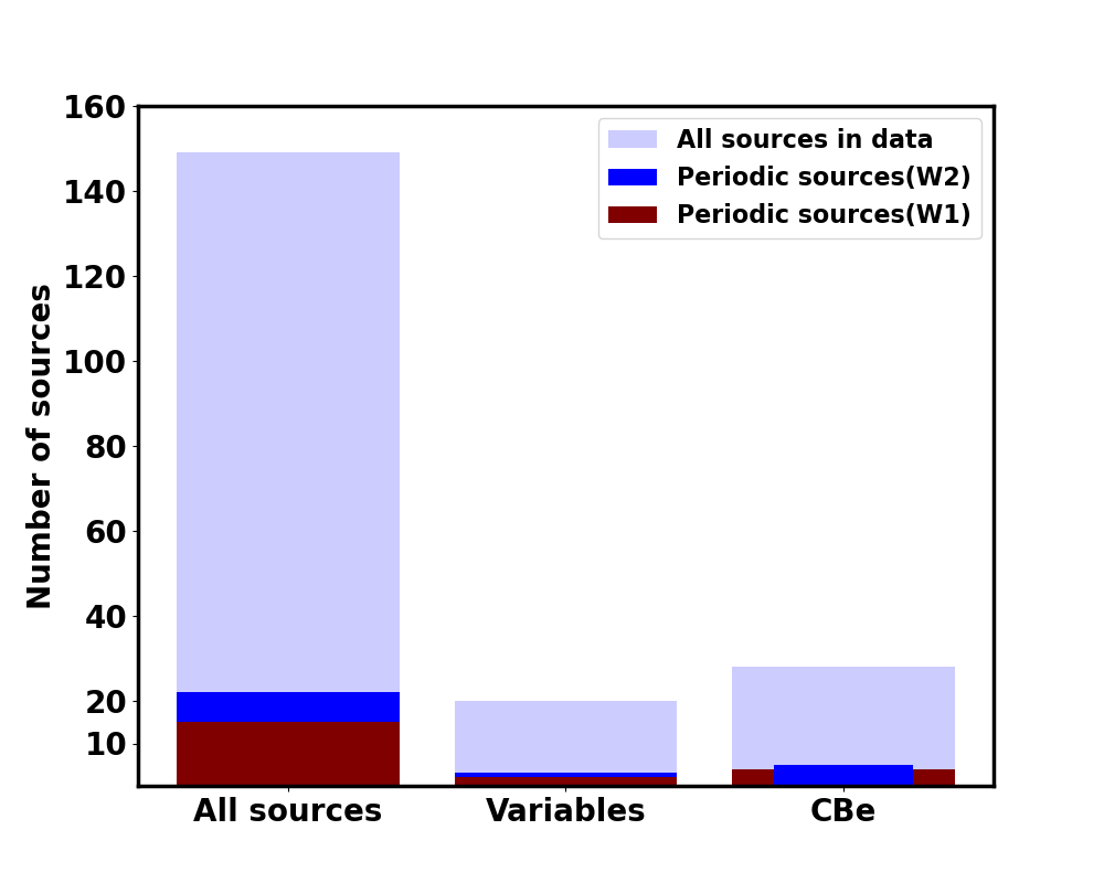
Figure 12: Bar plot showing the relative number of periodic sources for all sources, variables, and CBe stars present in NEOWISE data.

Table 3 represents a summary of the variability analysis using NEOWISE data. A detailed table for all the NEOWISE counterparts showing the variability and Periodicity analysis results can be found in the Appendix (Table 7).

Criteria	Subtype	Count (Non CBe | CBe | Red SG)
	Strong	6 | 11 | 0
Stetson Index (J)	Moderate	1 | 1 | 0
	Low	1 | 0 | 0
	Periodic	11(W1), 17(W2) | 4(W1), 5(W2) | 0
Periodic Signal (Lomb Scargle, LS)
	Non Periodic/ Uncertain	110(W1), 104(W2) | 24(W1) , 23(W2) | 0

Table 3: NEOWISE variability summary

7 Discussion

7.1 Multi-timescale variability in Classical Be stars in optical(ZTF) and IR(NEOWISE)

The variability observed in CBe stars can arise due to a variety of reasons. The Balmer emission of such stars is transient (Collins, 1987). Thus, they can transition from behaving like a Be star to a normal B-type star during disk dissipation or formation, which manifests as a rapid increase (outburst) or decrease (decay) in brightness followed by a slow return to baseline, spanning weeks to decades. The visual changes (outburst or decay) in the light curve due to these processes also depend on whether the star in question is being observed pole-on or edge-on (Rivinius et al., 2013). Then there are quasi-periodic variations on intermediate timescales of months to years due to wave motions in the decretion disk or binarity (Hayasaki & Okazaki, 2006; Carciofi et al., 2009). Finally, there is variability due to stellar non-radial pulsation (Labadie-Bartz et al. (2022b)) and/or rotation (Balona, 2022), which can have timescales between 0.2 and 3 days. Sources, where the dominant source of variability is from pulsation, are defined as "$\lambda$ Eri variables". This type of variation due to pulsation/rotation is more easily detectable using space-based observations compared to ground-based observations (Baade et al., 2016). Low-frequency stochastic variation is another feature of the power spectra of CBe stars. These signals typically show up as red noise at the lowest frequencies, but they have an astrophysical origin (Nazé et al., 2020).

We performed the Lomb Scargle analysis from section 5.3 for just CBe stars using both NEOWISE and ZTF lightcurves to search for the above-mentioned types of variations (periodic or not) in different timescales ranging from 0.2 to 3 days (pulsation), 7 days to 150 days (short term disk formation or dissipation or binarity or wave motions in decretion disk). We also look for CBe sources that show clear variations on timescales of weeks to decades due to disk formation or dissipation by eye. Many CBe stars contain more than one type of these variations, confirming a well-established notion from previous literature (Walker et al. 2005; Labadie-Bartz et al. 2022a).

For ZTF $r$-band data, out of 44 CBe sources, 6 CBe stars show a periodic signal in the typical pulsation/rotation range of 0.3 to 2 days, while 9 CBe stars have a periodic signal on timescales typically seen in quasi-cyclic variability due to wave motions in disk similar to $\omega$ CMa (B2V) (Stefl et al., 2010) and/or binarity. In addition, by manually inspecting the lightcurves by eye, we detect 4 additional sources showing variations due to disk alternating disk growth and decay /quasi-cyclic variations/binarity and 6 long-term variations related to disk loss or formation episodes, the latter being on the timescales of years. Labadie-Bartz et al. (2022a) showed that almost all CBe stars show grouped multi-periodicity near the pulsation timescales, which was already believed to be the case (Walker et al., 2005). Many sources in this work show more than one type of variation in different timescales, which is quite common for CBe stars (Rivinius et al., 2013). Stochastic aperiodic signals are also very common in CBe stars (Labadie-Bartz et al., 2022a) and are difficult to analyze quantitatively. It should be noted that almost all CBe stars, regardless of spectral type, are known to pulsate and show multi-periodicity if analyzed with long duration, high cadence data (Rivinius et al., 2013), and thus the numbers reported here are in no way representative of the actual picture regarding CBe pulsation and their periodicity. However, these results still provide an accurate representation of the timescales of variability seen in CBe stars. Table 4 summarizes these results. Figure 13 shows a few ZTF and NEOWISE lightcurves of CBe stars showing disk dissipation/formation events and quasi-cyclic variations. Panels A, F, B, and G belong to 2 stars, showing clear long-term variations due to disk formation or dissipation. Panels C, H, D, and I are lightcurves of another 2 stars, which show alternating periods of disk growth or decay and/or quasi-cyclic variability. Finally, panels E and J belong to a CBe star, showing clear quasi-cyclic variability on timescales of around 400 days.

Spectral classification from previous studies (Caron et al. 2003b; Subramaniam et al. 2006; Mathew & Subramaniam 2011; Marco & Negueruela 2013) and our own, we find that all of the 6 CBe stars that show periodic non-radial pulsation are early-type stars, which agrees with the fact that only early-type CBe stars pulsate strongly enough to be detected by ground-based telescopes with late-type stars sometimes showing pulsation with very small amplitudes (Rivinius et al., 2013). Among those stars that show variability on timescales seen due to alternate disk growth/dissipation or wave motion in disk and/or binarity, 11 out of 13 are early type, and 2 are mid type. Of those stars, we visually confirm to show variability due to long-term disk formation or dissipation events, 3 out of the 6 are early type, and the other 3 are mid type.

Similar to the above analysis using ZTF data, we perform the same using NEOWISE lightcurves for the 28 CBe cross matches present. Again we use a combination of visual inspection and a Lomb Scargle Periodogram to identify variability at different time scales. Out of the 28 CBe crossmatches in NEOWISE data, 4 stars show a clear periodic signal on the typical pulsation/rotation timescales of 0.2 and 3 days, all of which are early-types. One star shows a periodic signal on timescales of weeks or years from variability due to disk changes (formation/dissipation or wave-motion) or binarity. From visual inspection, we find 8 more stars with clear variability, either quasi-cyclic or due to alternating disk growth and decay or binarity. Thus, 9 CBe stars show variability in these timescales in infrared. 6 of these 9 stars are early-type, one is mid-type, two are late-type. 4 out of these 9 stars also show similar variability in optical wavelength (ZTF $r$ band). Finally, two stars (mid-type and early type) show clear long-term variations due to disk loss or formation from visual inspection. These two stars also show similar long-term variability in optical wavelength (ZTF $r$ band). All the trends in spectral types seen in infrared wavelength match well with previous findings mentioned in Rivinius et al. (2013) and Granada et al. (2018). A summary of the results is shown in Table 4.

To summarise the combined results of the variability of CBe stars identified using the data from ZTF and NEOWISE, 66% (29/44) of CBe counterparts are found to be variable. Our analysis finds that 23% (10/44) of CBe crossmatches show a periodic signal due to pulsation/rotation. Nearly all CBe stars studied to date are known to pulsate (Labadie-Bartz et al., 2022a; Rivinius et al., 2013). However, if these pulsations are non-sinusoidal or if the frequency peaks lie within the Window alias ranges described in section 5.3, the Lomb Scargle periodogram in this study might have not detected such signals. In addition, ZTF and NEOWISE lightcurves do not have a high enough cadence to successfully detect such high-frequency signals accurately most of the time. Neverthless, our analysis correctly represents the timescales of variability seen in CBe stars. We also find that 41% (18/44) CBe stars show variability due to alternating disk growth and decay, wave motion in disk or binarity, and 14% (6/44) show long-term variations due to disk dissipation/formation.

We use previous studies (Caron et al. 2003b; Subramaniam et al. 2006; Mathew & Subramaniam 2011; Marco & Negueruela 2013) and our own estimation of spectral types of cluster members and find that CBe stars showing periodicity due to non-radial pulsation /rotation are all early type. Although the statistics are poor, the results agree with the fact that late-type CBe stars pulsate with very small amplitudes, and thus, variations are harder to detect. We also find 50% (3/6) of CBe stars showing long-term disk variations due to dissipation and formation to be early type and the remaining to be mid type. Even though statistics are poor, Labadie-Bartz et al. (2018) found that most long-term variations in CBe stars are seen in early-type stars. On the other hand, (Granada et al., 2018) concluded that early-type CBe stars host stable disks.

Variability Mechanism	ZTF	NEOWISE	Combined
	(Total=44)	(Total=28)	(Total=44)
(a)Periodic pulsation/ rotation (0.2 to 3 days))	6	4	10
b) Alternating disk growth and decay, Wave motion in disk, binarity (weeks to years)	13	9	18
c) Long-term disk dissipation/formation (years to decades)	6	2	6
Multi-timescale variation	5(ab), 1(ac), 3(bc)	1(ab)	6(ab), 1(ac), 3(bc)
Dominant	1(a), 6(b), 2(c)	3(a), 8(b), 2 (c)	4(a), 12(b) , 4(c)
Irregular, Non-periodic or Uncertain	28	14	20

Table 4: Summary of the variability of CBe stars showing either periodic signals or visually clear variations from ZTF and NEOWISE lightcuves. The letters in brackets indicate which types of variations are present for sources showing variations on multiple timescales and those showing only one kind of variation (dominant).

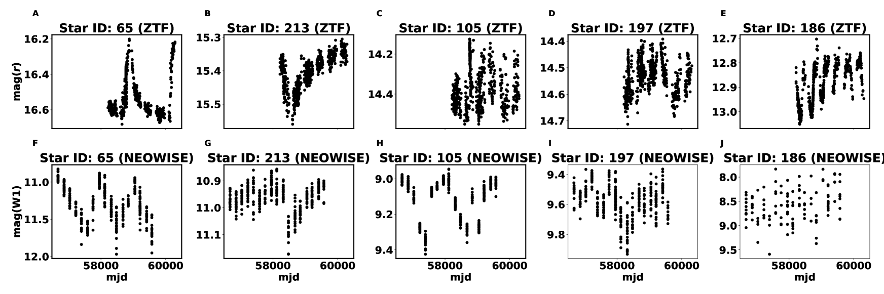
Figure 13: Lightcurves of 3 CBe stars, showing different kinds of magnitude variations. The top and bottom rows indicate ZTF and NEOWISE light curves for each star, respectively. For stars 65 and 213 (panels A, F, and B, G), we see clear long-term variations in timescales seen typically due to disk formation or dissipation. The brightening (outburst) and dimming (decay) of these 2 stars happens on much shorter timescales compared to their return to the baseline, which is typical for these kinds of variations (Haubois et al. 2012). Stars 105 and 197 (panels C, H, and D, I) show alternating periods of disk growth or decay and/or quasi-cyclic variability. Star 186 (panels E and J) shows clear quasi-cyclic variability on timescales of around 400 days.

7.2 Correlation between WISE color-color diagrams and CBe star properties

Near-IR excess in CBe stars compared to normal B-type stars has been detected for a long time, the first being in Johnson (1967). This excess was attributed to free–free and bound-free processes in the circumstellar material (gaseous disks) around these Be stars (Dougherty et al., 1994). Useful global information and trends for Be star’s life stage, spectral type, and variability can be obtained from its color excess in a color-color diagram (Granada et al., 2018). Recent works like Jian et al. (2024) find results in agreement with Granada et al. (2018).

We adopt the conditions given in Granada et al. (2018) for the color excess in WISE bands for classifying the active and quiescent CBe stars as well as the conditions from Nikutta et al. (2014) for the naked or normal B-type stars. We also look for any possible trends in the variability of candidate CBe stars from our earlier analysis using both ZTF and NEOWISE data. The WISE color-color plot is shown in fig. 14. Crossmatching WISE data with candidate CBe stars in ZTF and NEOWISE data resulted in 29 cross-matches.

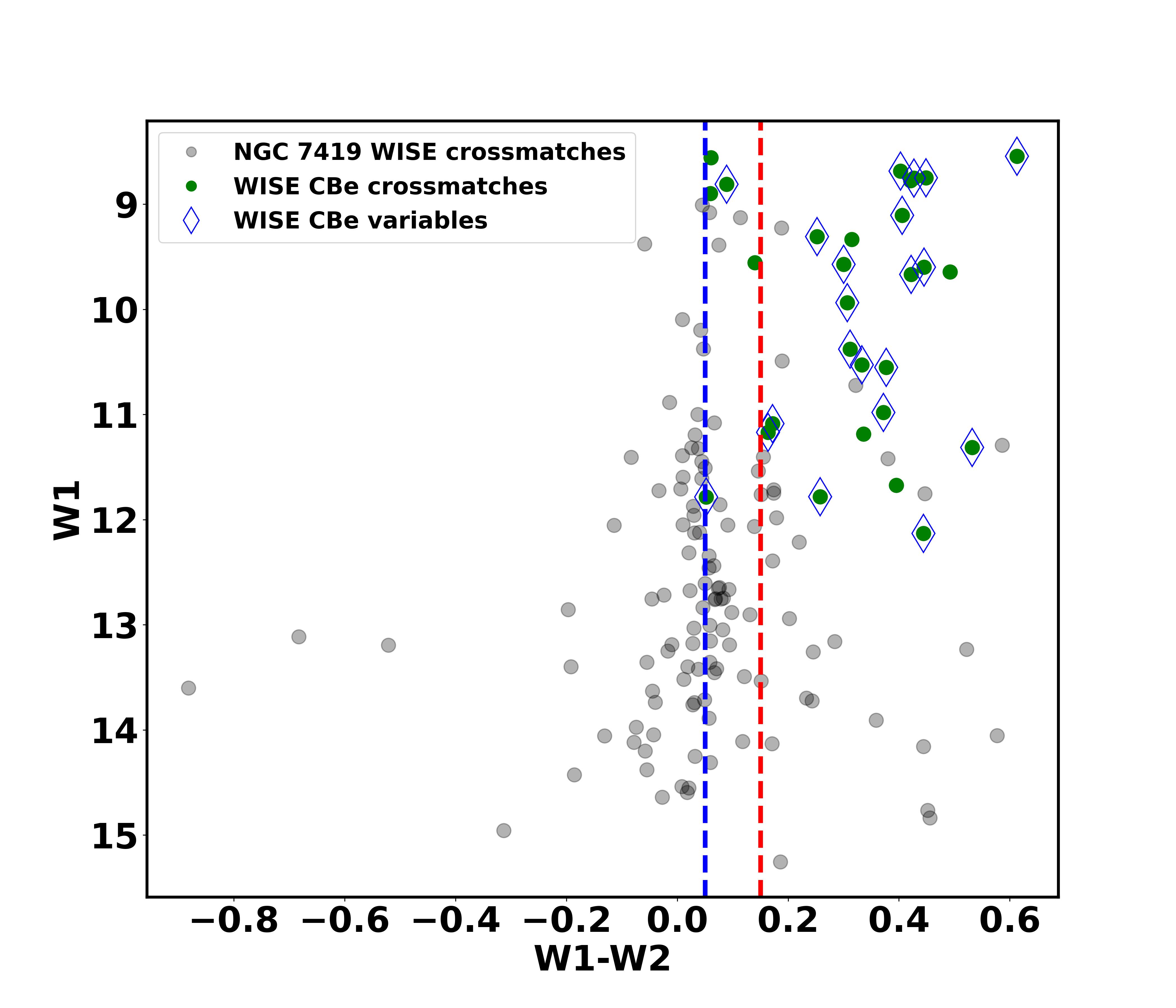
Figure 14: Color magnitude diagram with variability information for known and candidate CBe stars in NGC 7419. All known and candidate Be stars are indicated with green dots. The color limit (W1-W2 < 0.05) for normal B-type stars is shown by the dashed vertical blue line. The three regions namely, quiescent (no disk), active dissipating disk, and active stable disk for CBe stars are marked with dashed blue and red vertical lines with the W1-W2 limits as follows: Quiescent: W1-W2 <0.05, Active dissipating disk: 0.05 $\leq$ W1-W2 $\leq$ 0.15 and Active stable disk: W1-W2 > 0.15 (Granada et al., 2018).

We find that in NGC 7419, 83% of CBe stars have a high likelihood to have well-formed stable disks (W1-W2 > 0.15) while 17% lie in the dissipating disk (0.05 $\leq$ W1-W2 $\leq$ 0.15) region (see Granada et al. 2018). Interestingly, none of the candidate CBe stars lie in the quiescent region. This can be attributed to the fact that the detection of CBe stars with color excess increases with wavelength (Dougherty et al., 1991), and hence, the CBe stars in the quiescent region may show color excess when we go to longer wavelengths. All the sources on the right of the dashed blue line in fig. 14 can be used in the future as a test bed for detecting remaining CBe stars in this cluster, if any.

According to Granada et al. (2018), variable CBe stars are found in stars undergoing disk changes (0.05 $\leq$ W1-W2 $\leq$ 0.15) but predominantly in the active phase (W1-W2 $\geq$ 0.05). We find that all variable CBe stars belong to the active region except 2, which belong to the disk dissipating region.

From our spectral type estimation in section 3.3 and previous studies (Caron et al. 2003b; Subramaniam et al. 2006; Mathew & Subramaniam 2011; Marco & Negueruela 2013) , we see that, among the CBe stars in the active region (W1-W2>0.15), 83.3% are early, 8.3% are mid, and 8.3% are late-type B stars. 4 out of 5 sources in the disk dissipating region (0.05<W1-W2$\leq$0.15) are early-type and 1 is mid-type. According to Granada et al. (2018), early-type CBe stars host disks and are more likely to be in the active region. The low number of known late-type CBe stars with disks can be justified because they are harder to detect spectroscopically since only some show positive equivalent widths in the models described in Granada et al. (2018). In addition, late-type CBe stars possess less dense disks (Vieira et al., 2017) and hence exhibit lower IR emission.

We see similar numbers for variable CBe WISE counterparts. We find that most are early B-type (81%), with 9.5% being mid and 9.5% being late type. Hence, we observe that CBe stars (variable or not) are mostly early B-type stars, although this can be an observational bias due to late-type stars being harder to detect due to being less bright and possessing less denser disks. An explanation for why CBe stars are more likely to be early-type stars has been described in Rivinius et al. (2013). When the rotational velocity ($v_{\rm rot}$) at the equator and orbital velocity ($v_{orb}$) at the equator of a star are equal, it is said to be rotating critically. The ratio of $v_{rot}$ to $v_{orb}$ is defined as $W$, which signifies the velocity boost required for a given star to eject material into orbit.

$$W=\frac{v_{rot}}{v_{orb}}$$

.

According to Townsend et al. 2004; Rivinius, Th. et al. 2006 and Frémat et al. 2005, the mean value of $W$ is around 0.75 for CBe stars, with the minimum being 0.62 for a B type star to be classified as a CBe star. The mean and the cutoff $W$ value did not show any trend with effective temperature from star to star. Finally, according to Huang et al. (2010), low-mass B stars (late types; $<4M_{\odot}$) require a high threshold of $W$ > 0.96 to become Be stars. As stellar mass increases, this threshold decreases, dropping to 0.64 for early B stars with $M>8.6M_{\odot}$. This implies that early B-type stars have a much higher probability of being a CBe type since the mean value is much closer to the cut-off value for $W$, which is 0.62. This is in accordance with the distribution of Be stars within NGC 7419, which are generally brighter and early types.

8 Summary

We studied the open cluster NGC 7419, which stands out due to its high number of CBe stars and 5 Red Supergiants. Even though spectroscopic analysis of cluster members has been done in previous literature (Marco & Negueruela 2013; Subramaniam et al. 2006), no study has examined the variability of these members.

Following the footsteps of previous studies on cluster membership using both supervised and unsupervised algorithms, we use a combination of the Gaussian Mixture model and Random Forest algorithms on Gaia DR3 data for the open cluster NGC 7419 to find its high probability members. Using Gaia parallaxes and later comparing the inverse parallax distance with the Bailer-Jones distance (Bailer-Jones et al., 2021a), we estimate the average distance to the cluster to be around 3.6 $\pm$ 0.7 $kpc$. Next, using stellar evolutionary tracks from the PARSEC model, we determine the average age of the cluster to be $\approx$ $21.1^{+1.6}_{-0.6}$ Myr with a visual extinction of 5.2 mag. We use the modified table of Pecaut & Mamajek (2013) to estimate the mass an spectral type of cluster members. Combining this with previously known B-type stars from Caron et al. 2003b; Subramaniam et al. 2006; Mathew & Subramaniam 2011; Marco & Negueruela 2013, we find majority of our members (75%) to be B-type stars.

Based on $H\alpha$ photometric excess and using the synthetic tracks from Drew et al. (2005), and adopting a method similar to that described in Barentsen et al. (2011), we identify a total of 42 sources showing $H\alpha$ excess in the cluster, which is in agreement with a previous work by Paul Schmidtke and Tim Hunter (Schmidtke & Hunter, 2019). Given the age of the cluster, these sources cannot be Herbig Ae/Be type stars (Kiss et al., 2006) and are thus classified as candidate CBe stars as the decretion disk is directly related to the emission of $H\alpha$ lines in these stars (Rivinius et al., 2013). Combined with the list of previously known CBe stars, this brought the number of candidate CBe stars to 49 in the cluster, which is high for young open clusters. We find the ratio of CBe to (B+CBe) members to be 12.2% with majority of CBe stars being early-type.

Following this, we perform an extensive search for variable stars using data from both ground-based (ZTF, optical) and space-based (NEOWISE, infrared). We use 3 different methods, namely standard deviation, Median absolute deviation, and Stetson Index (Stetson (1996)), to identify high-probability variables in the cluster. We find 66% (29/44) of the candidate CBe stars in NGC 7419 CBe stars to be variable in either optical, infrared or both. Of the five supergiants, one (V* My Cep) is classified as variable in optical. All supergiants in NEOWISE data have magnitudes beyond the saturation limit and, hence, cannot be analyzed. Our method and thresholds for identifying variables are quite stringent, and hence, we are unable to identify very low amplitude variables as those sources may have high Stetson Index due to a high correlation between the variation in the two bands. However, the amplitude of variation being low causes those sources to have quite low values of standard deviation and median absolute deviation.

We then use the Generalised Lomb Scargle periodogram (Lomb 1976; Scargle 1982; VanderPlas 2018; Zechmeister & Kürster 2009) to search for stars showing periodic signals. Following the suggestions given in VanderPlas 2018; Kramer et al. 2023, and Ansdell et al. 2017b, we search for periodic signals in both ZTF and NEOWISE crossmatches in the cluster. The results of this analysis are given in Table 2 and 3. Since CBe stars are objects of special interest in this work, we take a deeper look into the various types of variability seen in these stars on different timescales in section 7.1. Due to computational constraints, we only look for periods up to 150 days, and sources with even longer periods will be looked at in future works.

We investigate variability in CBe stars across different timescales. Our analysis reveals that 23% (10/44) of CBe stars exhibit periodic signals from pulsation or rotation. While most known CBe stars pulsate (Labadie-Bartz et al., 2022a; Rivinius et al., 2013), non-sinusoidal periodic signals or frequency overlaps with the Window function (5.3) may affect the period detection by the Lomb-Scargle periodogram. Additionally, ZTF and NEOWISE lightcurves often lack the cadence to capture high-frequency signals. Nonetheless, we effectively represent the variability timescales in CBe stars. We also observe that 41% (18/44) of CBe stars show variability linked to disk dynamics or binarity, and 14% (6/44) exhibit long-term variations due to disk formation/dissipation.

Trends in spectral types align with prior studies (Rivinius et al., 2013; Granada et al., 2018), with all stars showing periodicity due to non-radial pulsation being early-type, consistent with the lower pulsation amplitudes seen in late-type CBe stars. Among the stars with long-term disk variations, we find 50% (3/6) are early-type and the other 3 are mid-type. Labadie-Bartz et al. (2018) found a similar percentage (57%) in long-term variations due to outbursts in early types. On the contrary, Granada et al. (2018) predicts early-type CBe stars to possess stable disks. Future spectroscopic studies on the candidate CBe stars identified in this work, along with better cadence and longer-duration light curves, will improve our understanding of these stars.

Finally, to obtain global information and trends for a Be star’s life stage, spectral type, and variability, we use WISE color-magnitude diagrams in a method similar to Granada et al. (2018). We observe that CBe stars exclusively lay in the region defined by W1-W2>0.05, which comes from the fact that the Be phenomenon is known to redden the star (Rivinius et al., 2013). We also find that most CBe stars (variable or not) have an early spectral type, but this may be an observational bias. It is argued in Rivinius et al. (2013) why CBe stars are more likely to be early-type.

Data Availability

The data used in this paper are available as follows:

ZTF (dr18): https://www.ztf.caltech.edu/ztf-public-releases.html

WISE and NEOWISE: https://irsa.ipac.caltech.edu/cgi-bin/Gator/nph-scan?submit=Select&projshort=WISE

IPHAS: https://vizier.cds.unistra.fr/viz-bin/VizieR?-source=IPHAS2

The full version of the various tables in this paper can be found online.

Appendix A Figures

Appendix B Tables

StarID	ra${}_{\textbf{J2016}}$	dec${}_{\textbf{J2016}}$	$\pi$ (mas)	$\mu_{\text{ra}}$ (mas/yr)	$\mu_{\text{dec}}$ (mas/yr)	magG	magBP	magRP	Membership probability
1	343.17621	60.83888	0.3405	-2.744	-1.685	19.09	20.58	17.91	0.915
2	343.17645	60.84831	0.2748	-2.626	-1.807	16.33	17.64	15.20	0.976
3	343.23409	60.85325	0.4212	-2.711	-1.61	17.37	18.97	16.16	0.908
4	343.24672	60.82561	0.2676	-2.749	-1.729	15.75	17.35	14.53	0.930
5	343.25140	60.91139	0.2295	-2.889	-1.636	16.61	17.73	15.53	0.933
6	343.26184	60.76568	0.1711	-2.896	-1.951	17.99	19.51	16.80	0.931
7	343.29404	60.94917	0.2488	-2.929	-1.756	17.76	18.82	16.74	0.928
8	343.35317	60.91576	0.2409	-2.664	-1.632	16.71	17.89	15.62	0.941
9	343.36459	60.80258	0.2685	-2.708	-1.546	17.35	18.87	16.19	0.972
10	343.37080	60.80499	0.278	-2.693	-1.454	13.36	14.73	12.21	0.962
11	343.37969	60.81559	0.2412	-2.612	-1.66	18.84	20.34	17.64	0.949
12	343.39324	60.80860	0.245	-2.783	-1.619	16.41	17.71	15.28	0.974
13	343.39678	60.91958	0.2818	-2.535	-1.666	18.36	19.66	17.24	0.910
14	343.39711	60.95327	0.2668	-2.818	-1.486	18.19	19.15	17.14	0.918
15	343.39741	60.81313	0.3344	-2.52	-1.323	19.02	20.51	17.85	0.920
16	343.40341	60.82153	0.3988	-2.685	-1.782	18.99	20.53	17.82	0.912
17	343.40753	60.78614	0.3147	-2.625	-1.746	17.58	19.05	16.41	0.967
18	343.41131	60.81780	0.3632	-2.607	-1.498	18.23	19.73	17.03	0.966
19	343.42137	60.73835	0.2815	-2.74	-1.814	13.58	14.58	12.57	0.912
20	343.43839	60.83333	0.3262	-2.69	-1.722	15.59	17.17	14.36	0.968
21	343.44087	60.85238	0.1648	-3.118	-1.549	20.22	21.40	19.00	0.932
22	343.44198	60.76308	0.1611	-2.873	-1.578	18.55	19.88	17.42	0.952
23	343.44434	60.86986	0.2899	-2.725	-1.529	14.22	15.43	13.13	0.964
24	343.44444	60.86876	0.3255	-2.946	-1.52	18.28	19.44	17.04	0.916
25	343.44788	60.84399	0.3365	-2.838	-1.481	18.75	20.22	17.55	0.966
26	343.44989	60.81892	0.2863	-2.875	-1.803	18.17	19.68	16.99	0.979
27	343.45053	60.78380	0.3134	-2.683	-1.514	17.74	19.06	16.61	0.994
28	343.45099	60.80874	0.2456	-2.655	-2.026	18.47	19.67	17.32	0.977
29	343.45291	60.80851	0.3043	-2.799	-1.779	18.47	19.83	17.32	0.984
30	343.45386	60.77529	0.339	-2.509	-1.449	18.36	19.68	17.24	0.989
31	343.45527	60.80658	0.3948	-2.535	-1.799	18.63	19.98	17.49	0.955
32	343.45531	60.79803	0.3519	-2.782	-1.598	19.54	21.09	18.35	0.952
33	343.45975	60.94957	0.3522	-2.691	-1.43	17.66	18.84	16.58	0.952
34	343.46037	60.89032	0.2974	-2.681	-1.52	15.74	16.91	14.66	0.960
35	343.46150	60.78477	0.2158	-2.856	-1.923	18.53	19.82	17.32	0.963
36	343.46301	60.79751	0.3829	-2.814	-1.658	19.00	20.64	17.79	0.963
37	343.46530	60.76785	0.1925	-2.495	-1.28	17.95	19.29	16.78	0.975
38	343.46664	60.82503	0.2782	-2.663	-1.626	15.08	16.61	13.88	0.995
39	343.46687	60.82660	0.2994	-2.731	-1.724	14.68	16.26	13.46	0.982
40	343.46798	60.76442	0.2829	-2.86	-1.744	15.61	16.96	14.47	0.997
41	343.47187	60.80232	0.2806	-2.742	-1.582	16.35	17.84	15.15	0.998
42	343.47491	60.81070	0.3749	-2.48	-1.494	19.19	20.78	17.97	0.928
43	343.47540	60.83323	0.3316	-2.943	-1.566	18.34	19.92	17.11	0.980
44	343.47752	60.81868	0.1793	-2.895	-1.394	19.37	20.82	18.14	0.934
45	343.47848	60.83771	0.1685	-2.44	-1.478	17.28	18.88	16.06	0.958
46	343.47965	60.80357	0.2093	-2.75	-1.768	16.66	18.03	15.51	0.988
47	343.48064	60.83338	0.3352	-2.708	-1.36	15.97	17.43	14.79	0.996
48	343.48269	60.82119	0.3899	-2.628	-1.565	17.62	19.20	16.42	0.989
49	343.48517	60.78986	0.2654	-2.708	-1.364	19.11	20.92	17.85	0.939
50	343.48768	60.79573	0.2846	-2.639	-1.493	17.04	18.63	15.82	0.964

Table 5: Sample table of NGC 7419 members from our membership analysis using Gaia DR3 data.
(The entire table will be available online.)

StarID	oid	ra${}_{\textbf{J2000}}$	dec${}_{\textbf{J2000}}$	magr	Stetson_Index	Variable	period (days)
2	831206400008687	343.17646	60.84832	16.51	69.07	0
3	831206400008544	343.23408	60.85326	17.68	45.11	0
4	831206400009263	343.24673	60.82562	16.07	63.40	0
5	831206400007191	343.25140	60.91140	16.72	97.35	0	2.45
7	831206400006239	343.29403	60.94918	17.85	44.92	0
8	831206400007031	343.35317	60.91577	16.84	41.26	0
9	831206400009812	343.36460	60.80259	17.59	55.66	0
10	831206400009734	343.37081	60.80500	13.57	69.18	0
12	831206400009594	343.39325	60.80861	16.56	149.72	1
17	831206400031822	343.40753	60.78615	17.85	57.93	0
19	1837214300027110	343.42137	60.73836	13.64	14.74	0
20	831206400008914	343.43840	60.83334	15.92	328.13	1	2.7105
23	831206400008010	343.44435	60.86987	14.36	73.26	0
27	831206400010299	343.45053	60.78381	17.93	31.90	0
33	831206400006113	343.45974	60.94958	17.78	34.88	0
34	831206400007521	343.46038	60.89033	15.86	24.53	0
38	831206400009115	343.46665	60.82504	15.36	100.07	0
39	831206400009066	343.46688	60.82661	14.99	97.13	0
40	831206400010824	343.46799	60.76443	15.82	48.93	0
41	831206400009729	343.47188	60.80233	16.59	196.18	1
45	831206400008752	343.47848	60.83772	17.58	28.27	0
46	831206400031554	343.47965	60.80358	16.87	50.28	0
47	831206400008884	343.48065	60.83339	16.21	10.56	0
48	831206400009207	343.48268	60.82120	17.96	33.36	0
50	831206400009915	343.48768	60.79574	17.34	53.73	0
53	831206400009455	343.49104	60.81177	17.66	51.59	0
59	831206400009672	343.50006	60.80298	16.48	54.76	0
60	831206400012445	343.50022	60.70457	16.61	32.49	0
61	831206400008183	343.50028	60.86170	12.77	32.22	0
62	831206400008560	343.50052	60.84548	16.00	8.84	0
65	831206400010604	343.50607	60.77160	16.51	830.09	1	0.4062, 9.5742
66	831206400009567	343.50797	60.80672	17.51	60.01	0
67	831206400054424	343.50806	60.80443	16.20	61.04	0
71	831206400012136	343.51038	60.71466	17.20	42.96	0
72	831206400031912	343.51042	60.77723	16.63	66.73	0
74	831206400009618	343.51199	60.80451	13.94	105.32	0	2.1015
76	831206400011065	343.51270	60.75437	17.23	36.40	0
77	831206400008437	343.51536	60.85033	17.60	67.10	0
80	831206400008546	343.51765	60.84568	17.98	13.07	0
81	831206400009970	343.51814	60.79327	17.37	79.32	0
82	831206400009216	343.51834	60.81988	13.12	90.95	0
83	831206400032114	343.51924	60.76122	16.15	109.36	0
84	831206400011437	343.51936	60.74037	17.96	31.10	0
86	831206400008902	343.52016	60.83180	16.54	48.58	0
87	831206400031461	343.52021	60.80849	17.36	26.74	0
88	831206400043581	343.52077	60.71451	16.26	45.10	0
89	831206400030865	343.52148	60.85359	17.38	24.63	0
92	831206400008979	343.52242	60.82831	16.47	23.02	0
94	831206400007101	343.52300	60.90815	16.30	56.35	0
97	831206400008593	343.52716	60.84310	16.99	63.65	0

Table 6: Sample variability and periodicity table for NGC 7419 members using ZTF $r$ band data. StarID corresponds to the ID assigned during membership in section 3. Variable and non-variable stars are indicated by 1 and 0, respectively, in the variable column. (The entire table will be available online.)

StarID	ra${}_{\textbf{J2000}}$	dec${}_{\textbf{J2000}}$	mag${}_{\text{W1}}$	mag${}_{\text{W2}}$	Stetson_Index	Variable	period${}_{\text{W1}}$ (days)	period${}_{\text{W2}}$ (days)
1	343.17617	60.83897	14.24	14.10	10.46	0	-	-
2	343.17649	60.84832	12.18	12.15	41.34	0	-	-
3	343.23413	60.85326	12.79	12.75	53.33	0	-	-
4	343.24672	60.82562	11.09	11.05	63.99	0	-	-
5	343.25144	60.91136	12.75	12.74	87.64	0	-	-
6	343.26189	60.76569	13.60	13.65	48.33	0	-	-
7	343.29399	60.94918	14.34	14.36	9.63	0	-	0.1651
8	343.35304	60.91573	12.66	12.63	77.25	0	-	-
10	343.37082	60.80501	9.09	9.03	200.80	0	-	-
12	343.39327	60.80861	12.38	12.39	93.90	0	-	-
13	343.39705	60.91960	14.04	14.07	29.74	0	-	103.9236
15	343.39731	60.81297	14.41	14.44	16.48	0	-	0.6096
16	343.40350	60.82162	13.88	13.29	37.36	0	-	0.1420
17	343.40754	60.78625	13.14	13.09	52.57	0	-	-
18	343.41168	60.81773	13.50	13.51	28.01	0	-	-
19	343.42137	60.73837	10.13	10.12	122.39	0	-	-
20	343.43842	60.83334	10.35	10.04	216.62	0	-	-
22	343.44211	60.76299	14.02	13.81	-28.48	0	-	-
23	343.44437	60.86984	10.39	10.36	57.08	0	-	-
25	343.44789	60.84399	14.22	14.32	8.14	0	-	-
26	343.44994	60.81895	13.67	13.72	-13.44	0	0.2327	1.0129
27	343.45058	60.78369	13.61	13.66	-10.91	0	-	-
28	343.45120	60.80854	13.31	13.36	6.01	0	1.9536	0.2177
30	343.45394	60.77512	13.96	13.85	-9.52	0	-	-
33	343.45969	60.94959	13.76	13.73	51.02	0	-	-
34	343.46040	60.89033	11.97	11.97	47.83	0	-	-
37	343.46499	60.76789	13.37	13.29	9.25	0	-	-
39	343.46689	60.82643	9.69	9.66	175.23	0	-	-
40	343.46798	60.76444	11.43	11.42	25.19	0	-	-
41	343.47187	60.80236	11.54	11.28	2653.07	1	-	-
43	343.47519	60.83321	13.30	13.29	25.18	0	-	-
45	343.47850	60.83771	12.58	12.56	129.24	0	-	-
46	343.47971	60.80353	12.49	12.23	-82.48	0	-	-
47	343.48063	60.83338	11.52	11.50	135.18	0	-	-
48	343.48259	60.82108	12.72	12.79	52.81	0	0.1519	-
51	343.48807	60.75563	13.70	13.73	36.22	0	-	-
52	343.48983	60.81768	13.45	13.50	-61.77	0	-	-
53	343.49112	60.81175	13.21	12.99	-59.82	0	-	-
54	343.49315	60.81591	13.63	13.77	-2.92	0	-	-
60	343.50031	60.70458	12.40	12.39	98.15	0	-	-
61	343.50029	60.86169	8.56	8.50	87.40	0	-	-
62	343.50038	60.84546	12.05	11.96	78.65	0	-	-
65	343.50609	60.77159	11.28	11.15	1860.56	1	-	-
71	343.51041	60.71462	12.87	12.82	108.09	0	-	-
72	343.51041	60.77717	11.84	12.09	173.09	0	-	-
74	343.51190	60.80454	9.67	9.76	95.06	0	-	-
76	343.51279	60.75438	13.07	13.11	116.85	0	-	-
77	343.51537	60.85025	13.08	13.09	5.11	0	-	-
80	343.51776	60.84556	13.72	13.59	32.34	0	-	-
82	343.51836	60.81988	9.02	9.02	67.17	0	-	-

Table 7: Sample variability and periodicity table for NGC 7419 members using NEOWISE 2 band data. StarID corresponds to the ID assigned during membership in section 3. Variable and non-variable stars are indicated by 1 and 0, respectively, in the variable column.
(The entire table will be available online.)

References

- Ansdell et al. (2017a) Ansdell M., et al., 2017a, Monthly Notices of the Royal Astronomical Society, 473, 1231
- Ansdell et al. (2017b) Ansdell M., et al., 2017b, Monthly Notices of the Royal Astronomical Society, 473, 1231
- Baade et al. (2016) Baade D., et al., 2016, A&A, 588, A56
- Bailer-Jones et al. (2021a) Bailer-Jones C. A. L., Rybizki J., Fouesneau M., Demleitner M., Andrae R., 2021a, VizieR Online Data Catalog, p. I/352
- Bailer-Jones et al. (2021b) Bailer-Jones C. A. L., Rybizki J., Fouesneau M., Demleitner M., Andrae R., 2021b, AJ, 161, 147
- Balona (2022) Balona L. A., 2022, MNRAS, 516, 3641
- Baluev (2008) Baluev R. V., 2008, MNRAS, 385, 1279
- Barentsen et al. (2011) Barentsen G., et al., 2011, MNRAS, 415, 103
- Barentsen et al. (2014) Barentsen G., et al., 2014, Monthly Notices of the Royal Astronomical Society, 444, 3230
- Beauchamp et al. (1994) Beauchamp A., Moffat A. F. J., Drissen L., 1994, ApJS, 93, 187
- Bellm et al. (2018) Bellm E. C., et al., 2018, Publications of the Astronomical Society of the Pacific, 131, 018002
- Bhatt et al. (1993) Bhatt B. C., Pandey A. K., Mohan V., Mahra H. S., Paliwal D. C., 1993, Bulletin of the Astronomical Society of India, 21, 33
- Bishop (2006) Bishop C. M., 2006, Pattern Recognition and Machine Learning (Information Science and Statistics). Springer-Verlag, Berlin, Heidelberg
- Breiman (2001) Breiman L., 2001, Random Forests
- Bressan et al. (2012) Bressan A., Marigo P., Girardi L., Salasnich B., Dal Cero C., Rubele S., Nanni A., 2012, MNRAS, 427, 127
- Carciofi (2011) Carciofi A. C., 2011, IAU Symp., 272, 325
- Carciofi et al. (2009) Carciofi A. C., Okazaki A. T., Le Bouquin J. B., Štefl S., Rivinius T., Baade D., Bjorkman J. E., Hummel C. A., 2009, A&A, 504, 915
- Caron et al. (2003a) Caron G., Moffat A. F. J., St-Louis N., Wade G. A., Lester J. B., 2003a, AJ, 126, 1415
- Caron et al. (2003b) Caron G., Moffat A. F. J., St-Louis N., Wade G. A., Lester J. B., 2003b, AJ, 126, 1415
- Chen et al. (2020) Chen X., Wang S., Deng L., de Grijs R., Yang M., Tian H., 2020, VizieR Online Data Catalog: The ZTF catalog of periodic variable stars (Chen+, 2020), VizieR On-line Data Catalog: J/ApJS/249/18. Originally published in: 2020ApJS..249…18C, doi:10.26093/cds/vizier.22490018
- Cody et al. (2014) Cody A. M., et al., 2014, AJ, 147, 82
- Collins (1987) Collins G. W., 1987, International Astronomical Union Colloquium, 92, 3–21
- Cutri et al. (2012) Cutri R. M., et al., 2012, Explanatory Supplement to the WISE All-Sky Data Release Products, Explanatory Supplement to the WISE All-Sky Data Release Products
- Das et al. (2023) Das S. R., Gupta S., Prakash P., Samal M., Jose J., 2023, The Astrophysical Journal, 948, 7
- Dougherty et al. (1991) Dougherty S. M., Taylor A. R., Clark T. A., 1991, AJ, 102, 1753
- Dougherty et al. (1994) Dougherty S. M., Waters L. B. F. M., Burki G., Cote J., Cramer N., van Kerkwijk M. H., Taylor A. R., 1994, A&A, 290, 609
- Drew et al. (2005) Drew J. E., et al., 2005, MNRAS, 362, 753
- Dutta et al. (2015) Dutta S., Mondal S., Jose J., Das R. K., Samal M. R., Ghosh S., 2015, MNRAS, 454, 3597
- Frémat et al. (2005) Frémat Y., Zorec J., Hubert A. M., Floquet M., 2005, A&A, 440, 305
- Gaia Collaboration et al. (2016) Gaia Collaboration et al., 2016, A&A, 595, A1
- Gaia Collaboration et al. (2018a) Gaia Collaboration et al., 2018a, A&A, 616, A1
- Gaia Collaboration et al. (2018b) Gaia Collaboration et al., 2018b, A&A, 616, A10
- Gaia Collaboration et al. (2023) Gaia Collaboration et al., 2023, A&A, 674, A1
- Galli et al. (2020) Galli P. A. B., et al., 2020, A&A, 643, A148
- Granada et al. (2018) Granada A., Jones C. E., Sigut T. A. A., Semaan T., Georgy C., Meynet G., Ekström S., 2018, The Astronomical Journal, 155, 50
- Grundstrom et al. (2011) Grundstrom E. D., McSwain M. V., Aragona C., Boyajian T. S., Marsh A. N., Roettenbacher R. M., 2011, Bulletin de la Societe Royale des Sciences de Liege, 80, 371
- Gupta et al. (2024) Gupta S., Jose J., Das S. R., Guo Z., Damian B., Prakash P., Samal M. R., 2024, Monthly Notices of the Royal Astronomical Society, 528, 5633
- Haubois et al. (2012) Haubois X., Carciofi A. C., Rivinius T., Okazaki A. T., Bjorkman J. E., 2012, ApJ, 756, 156
- Hayasaki & Okazaki (2006) Hayasaki K., Okazaki A. T., 2006, MNRAS, 372, 1140
- Huang et al. (2010) Huang W., Gies D. R., McSwain M. V., 2010, The Astrophysical Journal, 722, 605
- Jian et al. (2024) Jian M., Matsunaga N., Jiang B., Yuan H., Zhang R., 2024, A&A, 682, A59
- Johnson (1967) Johnson H. L., 1967, ApJ, 150, L39
- Joshi et al. (2008) Joshi H., Kumar B., Singh K. P., Sagar R., Sharma S., Pandey J. C., 2008, Monthly Notices of the Royal Astronomical Society, 391, 1279
- Kee et al. (2015) Kee N., Owocki S., Townsend R., Müller H.-R., 2015, Pulsational Mass Ejection in Be Star Disks (arXiv:1412.8511), https://arxiv.org/abs/1412.8511
- Kiss et al. (2006) Kiss L. L., Szabo G. M., Bedding T. R., 2006, Monthly Notices of the Royal Astronomical Society, 372, 1721–1734
- Kozhurina-Platais et al. (1995) Kozhurina-Platais V., Girard T. M., Platais I., van Altena W. F., Ianna P. A., Cannon R. D., 1995, AJ, 109, 672
- Kramer et al. (2023) Kramer D., Gowanlock M., Trilling D., McNeill A., Erasmus N., 2023, Astronomy and Computing, 44, 100711
- Kroll & Hanuschik (1997) Kroll P., Hanuschik R. W., 1997, in Wickramasinghe D. T., Bicknell G. V., Ferrario L., eds, Astronomical Society of the Pacific Conference Series Vol. 121, IAU Colloq. 163: Accretion Phenomena and Related Outflows. p. 494
- Labadie-Bartz et al. (2018) Labadie-Bartz J., et al., 2018, AJ, 155, 53
- Labadie-Bartz et al. (2022a) Labadie-Bartz J., Carciofi A. C., Henrique de Amorim T., Rubio A., Luiz Figueiredo A., Ticiani dos Santos P., Thomson-Paressant K., 2022a, AJ, 163, 226
- Labadie-Bartz et al. (2022b) Labadie-Bartz J., Carciofi A. C., Henrique de Amorim T., Rubio A., Luiz Figueiredo A., Ticiani dos Santos P., Thomson-Paressant K., 2022b, AJ, 163, 226
- Lee et al. (1991) Lee U., Osaki Y., Saio H., 1991, MNRAS, 250, 432
- Lindegren et al. (2021) Lindegren L., et al., 2021, A&A, 649, A2
- Lomb (1976) Lomb N. R., 1976, Ap&SS, 39, 447
- Mainzer et al. (2011) Mainzer A., et al., 2011, ApJ, 743, 156
- Mainzer et al. (2014) Mainzer A., et al., 2014, ApJ, 792, 30
- Manoj et al. (2006) Manoj P., Bhatt H. C., Gopinathan M., Salim M., 2006, The Astrophysical Journal, 653
- Marco & Negueruela (2013) Marco A., Negueruela I., 2013, Astronomy & Astrophysics, 552, A92
- Marton et al. (2023) Marton G., et al., 2023, A&A, 674, A21
- Masci et al. (2018) Masci F. J., et al., 2018, Publications of the Astronomical Society of the Pacific, 131, 018003
- Mathew & Subramaniam (2011) Mathew B., Subramaniam A., 2011, Bulletin of the Astronomical Society of India, 39, 517
- Murphy (2012) Murphy K. P., 2012, Machine Learning: A Probabilistic Perspective. The MIT Press
- Navarete et al. (2024) Navarete F., Ticiani dos Santos P., Carciofi A. C., Figueiredo A. L., 2024, ApJ, 970, 113
- Nazé et al. (2020) Nazé Y., Rauw G., Pigulski A., 2020, MNRAS, 498, 3171
- Nikutta et al. (2014) Nikutta R., Hunt-Walker N., Nenkova M., Ivezić Ž., Elitzur M., 2014, MNRAS, 442, 3361
- Ochsenbein (1996) Ochsenbein F., 1996, The VizieR database of astronomical catalogues, doi:10.26093/CDS/VIZIER, https://vizier.cds.unistra.fr
- Ochsenbein et al. (2000) Ochsenbein F., Bauer P., Marcout J., 2000, A&AS, 143, 23
- Panoglou et al. (2016) Panoglou D., Carciofi A. C., Vieira R. G., Cyr I. H., Jones C. E., Okazaki A. T., Rivinius T., 2016, MNRAS, 461, 2616
- Panoglou et al. (2018) Panoglou D., Faes D. M., Carciofi A. C., Okazaki A. T., Baade D., Rivinius T., Borges Fernandes M., 2018, MNRAS, 473, 3039
- Pecaut & Mamajek (2013) Pecaut M. J., Mamajek E. E., 2013, ApJS, 208, 9
- Pedregosa et al. (2018) Pedregosa F., et al., 2018, Scikit-learn: Machine Learning in Python (arXiv:1201.0490), https://arxiv.org/abs/1201.0490
- Porter & Rivinius (2003a) Porter J. M., Rivinius T., 2003a, PASP, 115, 1153
- Porter & Rivinius (2003b) Porter J. M., Rivinius T., 2003b, PASP, 115, 1153
- Rímulo et al. (2018) Rímulo L. R., et al., 2018, MNRAS, 476, 3555
- Rivinius, Th. et al. (2006) Rivinius, Th. Stefl, S. Baade, D. 2006, A&A, 459, 137
- Rivinius et al. (1998) Rivinius T., Baade D., Stefl S., Stahl O., Wolf B., Kaufer A., 1998, A&A, 336, 177
- Rivinius et al. (2013) Rivinius T., Carciofi A. C., Martayan C., 2013, The Astronomy and Astrophysics Review, 21
- Sanders (1971) Sanders W. L., 1971, A&A, 14, 226
- Sarro et al. (2014) Sarro L. M., et al., 2014, A&A, 563, A45
- Scargle (1982) Scargle J. D., 1982, ApJ, 263, 835
- Schmidtke & Hunter (2019) Schmidtke P., Hunter T., 2019, Research Notes of the AAS, 3, 67
- Sokolovsky et al. (2016a) Sokolovsky K. V., et al., 2016a, Monthly Notices of the Royal Astronomical Society, 464, 274
- Sokolovsky et al. (2016b) Sokolovsky K. V., et al., 2016b, Monthly Notices of the Royal Astronomical Society, 464, 274
- Stefl et al. (2010) Stefl S., Rivinius T., Le Bouquin J. B., Carciofi A., Baade D., Otero S., Rantakyrö F., 2010, in Revista Mexicana de Astronomia y Astrofisica Conference Series. pp 89–91
- Stetson (1996) Stetson P. B., 1996, PASP, 108, 851
- Subramaniam et al. (2006) Subramaniam A., Mathew B., Bhatt B. C., Ramya S., 2006, Monthly Notices of the Royal Astronomical Society, 370, 743
- Townsend et al. (2004) Townsend R. H. D., Owocki S. P., Howarth I. D., 2004, Monthly Notices of the Royal Astronomical Society, 350, 189
- VanderPlas (2018) VanderPlas J. T., 2018, ApJS, 236, 16
- Vasilevskis et al. (1958) Vasilevskis S., Klemola A., Preston G., 1958, AJ, 63, 387
- Vieira et al. (2015) Vieira R. G., Carciofi A. C., Bjorkman J. E., 2015, MNRAS, 454, 2107
- Vieira et al. (2017) Vieira R. G., Carciofi A. C., Bjorkman J. E., Rivinius T., Baade D., Rímulo L. R., 2017, MNRAS, 464, 3071
- Virtanen et al. (2020) Virtanen P., et al., 2020, Nature Methods, 17, 261
- Walker et al. (2005) Walker G. A. H., et al., 2005, ApJ, 623, L145
- Welch & Stetson (1993) Welch D. L., Stetson P. B., 1993, AJ, 105, 1813
- Wright et al. (2010) Wright E. L., et al., 2010, AJ, 140, 1868
- Zechmeister & Kürster (2009) Zechmeister M., Kürster M., 2009, A&A, 496, 577