Re-Visible Dual-Domain Self-Supervised Deep Unfolding Network for MRI Reconstruction

Abstract

Magnetic Resonance Imaging (MRI) is widely used in clinical practice, but suffered from prolonged acquisition time. Although deep learning methods have been proposed to accelerate acquisition and demonstrate promising performance, they rely on high-quality fully-sampled datasets for training in a supervised manner. However, such datasets are time-consuming and expensive-to-collect, which constrains their broader applications. On the other hand, self-supervised methods offer an alternative by enabling learning from under-sampled data alone, but most existing methods rely on further partitioned under-sampled k-space data as model’s input for training, resulting in a loss of valuable information. Additionally, their models have not fully incorporated image priors, leading to degraded reconstruction performance. In this paper, we propose a novel re-visible dual-domain self-supervised deep unfolding network to address these issues when only under-sampled datasets are available. Specifically, by incorporating re-visible dual-domain loss, all under-sampled k-space data are utilized during training to mitigate information loss caused by further partitioning. This design enables the model to implicitly adapt to all under-sampled k-space data as input. Additionally, we design a deep unfolding network based on Chambolle and Pock Proximal Point Algorithm (DUN-CP-PPA) to achieve end-to-end reconstruction, incorporating imaging physics and image priors to guide the reconstruction process. By employing a Spatial-Frequency Feature Extraction (SFFE) block to capture global and local feature representation, we enhance the model’s efficiency to learn comprehensive image priors. Experiments conducted on the fastMRI and IXI datasets demonstrate that our method significantly outperforms state-of-the-art approaches in terms of reconstruction performance.

MRI reconstruction, self-supervised learning, Dual-domain, deep unfolding, re-visible

1 Introduction

Magnetic Resonance Imaging (MRI) is a widely employed medical imaging technique, known for its non-invasive approach, high resolution, and superior soft tissue contrast [36]. Besides, the integration of various imaging modalities provides additional insights into tissue and organ characteristics, improving diagnostic precision. However, acquisition of certain MRI modalities tend to be slow because of the repetitive signal spatial encoding and the constraints of the hardware. The prolonged acquisition time increases patient discomfort and leads to a higher accumulation of motion artifacts, which can degrade image quality and compromise diagnostic accuracy. Consequently, accelerating MRI acquisition is crucial for clinical practice. One effective approach [1] to achieve this is by reducing the amount of k-space data collected by a pre-defined pattern, and subsequently reconstructing fully-sampled images from under-sampled data.

CS-MRI techniques [2, 3, 4, 49] facilitate accurate image reconstruction from under-sampled data at sampling rates significantly below those dictated by the Nyquist sampling theorem. These methods typically leverage the sparsity of signals and optimization algorithms to significantly reduce the sampling rate requirements while still maintaining high image quality. Although theoretically sound, crafting an optimal regularizer remains a difficult task. Recent deep learning-based approaches [5, 6, 19, 37, 38, 39, 46, 47, 48] have shown promising results, enabling fast and accurate reconstructions. However, these methods are often ”black-boxes,” lacking interpretability and physical insight, which limits their clinical applications. To overcome this limitation, deep unfolding networks [7, 8, 9, 10, 11, 12, 20, 24, 40, 41] have been introduced. These networks combine the imaging physics and image priors by effectively unfolding the iterations of an optimization algorithm into deep neural networks, which enhances both interpretability and performance. Although deep unfolding networks have shown promise in MRI reconstruction, most approaches rely on supervised training on high-quality fully-sampled datasets. However, in clinical practice, collecting such datasets is both time-consuming and costly, may even be technically unfeasible, as it requires extended acquisition times, advanced equipment, and specialized expertise. For example, cardiovascular MRI is challenged by excessive involuntary movements, while diffusion MRI with echo-planar imaging suffers from rapid $T^{*}_{2}$ signal decay.

To address this limitation, self-supervised learning [13, 14, 15, 16, 17, 18, 21, 22, 23, 31, 44, 45], which enables learning from only under-sampled k-space data, has gained significant interest from researchers. For example, Huang et al. replace the under-sampled and fully-sampled training pairs with pairs of under-sampled data when training the network, reducing the dependence of model training on high-quality datasets to some extent [13]. However, obtaining pairs of under-sampled data is still quite challenging in practice. Some methods [14, 15, 16, 18, 22, 23] have been developed to enable training using only single under-sampled data. For instance, Yaman et al. divides the acquired k-space data into two disjoint sets, one used as the input and the other as the target for cross-validation [23]. Although the dependence on high-quality datasets has been significantly reduced, most existing methods rely on further partitioned under-sampled k-space data as input for training, resulting in a loss of valuable information. Additionally, their models have not fully incorporate image priors, leading to degraded reconstruction performance.

In this paper, we propose a re-visible dual-domain self-supervised deep unfolding network to address the aforementioned limitations. Our framework integrates a re-visible dual-domain self-supervised learning approach to mitigate information loss when only under-sampled datasets are available. Furthermore, it incorporates a deep unfolding network based on the Chambolle and Pock Proximal Point Algorithm (DUN-CP-PPA), embedding the imaging model directly into the reconstruction process to improve incorporation of image priors. Specifically, by introducing re-visible dual-domain loss, all under-sampled k-space data are utilized during training, effectively compensating information loss caused by further partitioning. This design allows the model to implicitly adapt to all under-sampled k-space data as input (make the information loss caused by further partitioning ”re-visible” to the model). Moreover, we employ DUN-CP-PPA to achieve end-to-end reconstruction, incorporating imaging physics and image priors to guide the reconstruction process by unfolding the optimization stages with network architecture. By introducing a Spatial-Frequency Feature Extraction (SFFE) block to capture both global and local feature representations, we improve the model’s ability to learn comprehensive image priors. The main contributions of this paper are listed as follows:

• We propose a re-visible dual-domain self-supervised deep unfolding network to improve reconstruction performance utilizing only under-sampled k-space data for training.

• We introduce a revisible dual-domain self-supervised learning approach, featuring the design of a re-visible dual-domain loss to compensate for the information loss caused by further partitioning during training. This design enables the model to implicitly adapt to all under-sampled k-space data.

• By unfolding each stage of CP-PPA with network modules, we embed imaging physics and image priors to guide the reconstruction process, resulting in DUN-CP-PPA. Additionally, we utilize SFFE block to improve the DUN-CP-PPA’s ability to learn comprehensive image priors.

• Through extensive experiments on both the fastMRI dataset and the IXI dataset, we show that the proposed model outperforms current state-of-the-art methods in terms of both quantitative metrics and qualitative visual reconstruction quality.

2 Related work

2.1 Chambolle and Pock Proximal Point Algorithm

The Chambolle and Pock Proximal Point Algorithm (CP-PPA) is an effective optimization technique [26, 27, 28] that employs a primal-dual hybrid approach [29] to ensure both convergence and efficiency. The original objective function:

$$\min_{x}f(x)+g(Lx),$$

is transformed into its primal-dual form:

$$\min_{x}\max_{y}f(x)+\langle Lx,y\rangle-g^{*}(y),$$

where $g^{*}$ is the convex conjugate of $g$, $L$ is a continuous linear operator . The KKT conditions for this problem are:

$$\left\{\begin{array}[]{l}-L^{H}y_{\star}\in\partial f(x_{\star}),\\ Lx_{\star}\in\partial g^{*}(y_{\star}),\end{array}\right.$$

where $L^{H}$ is the Hermitian transpose of $L$, CP-PPA solves the primal-dual problem iteratively using the update rules:

$$\left\{\begin{aligned} x_{k+1}&=\operatorname{Prox}_{f}^{\tau_{k+1}}\left(x_{k}-\tau_{k+1}L^{H}y_{k}\right),\\ y_{k+1}&=\operatorname{Prox}_{g^{*}}^{\sigma_{k+1}}(y_{k}+\sigma_{k+1}Lz_{k+1}).\end{aligned}\right.$$

where $z_{k+1}=x_{k+1}+\theta_{k+1}(x_{k+1}-x_{k})$. Compared to the Iterative Shrinkage/Thresholding Algorithm (ISTA) [30], CP-PPA converges faster and provides stronger theoretical guarantees for globally optimal solutions [28]. However, its performance is sensitive to the choice of parameters (e.g., $\alpha$ and $\beta$), and incorrect selection can lead to slow convergence or instability.

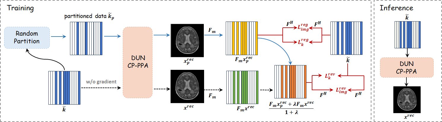
Figure 1: The framework of our proposed re-visible dual-domain self-supervised learning is shown. We utilize DUN-CP-PPA for reconstruction with image physics incorporated. During training, we adopt a dual-branch structure. The first branch reconstructs $\tilde{k}_{p}$ to boost the model’s generative capability and the second branch reconstructs $\tilde{k}$ to compensate information loss caused by further partitioning. The model is trained using the proposed re-visible dual-domain loss. During inference, the trained network can directly reconstruct the image from $\tilde{k}$.

2.2 Deep Unfolding Network

Deep unfolding networks effectively combine model-based optimization algorithms with data-driven learning approaches, providing a combination of the advantages of both approaches. They have attracted significant attention in recent years due to their impressive performance, especially in CS-MRI [7, 8, 9, 10, 11, 12].

In CS-MRI, Deep Unfolding Networks have demonstrated considerable success by unfolding various optimization techniques. ADMM-CSNet [10, 12, 13] casts the iterative Alternating Direction Method of Multipliers (ADMM) algorithm into a deep network architecture for image CS reconstruction. Integrating the Alternating Iterative Shrinkage-Thresholding Algorithm (ISTA) into the model design. Expanding Half-Quadratic Splitting (HQS) [7, 8, 9] with corresponding network modules. Different network modules can also enhance the capabilities of deep unfolding networks, such as CNNs and U-nets. [11] enhances the network’s ability to extract comprehensive features by incorporating channel and spatial attention modules. [25] proposes an Adaptive Local Neighborhood-based Neural Network that integrates with deep unfolding networks to improve reconstruction quality. [12] combines an elaborately designed reversible network to map inputs to a channel-lifted implicit space, boosting performance, and proposing a dual-domain update for better features fusion.

2.3 Self-Supervised Learning Methods

In order to get rid of dependence on fully-sampled data, self-supervised methods [13, 14, 15, 16, 17, 18, 21, 22, 23, 31] are proposed for MRI reconstruction, which are trained with under-sampled data. The classical k-space interpolation method[32, 33], which first fully samples a calibrated region in the central part of the k-space, learns a linear kernel and uses it in a translation-invariant manner to interpolate in the missing k-space data. Inspired by deep learning, linear kernels are generalized to convolutional neural networks[34, 35] to improve the accuracy of missing data interpolation. With the further development of self-supervised learning techniques, many works have also emerged in the field of MRI reconstruction. By further down-sampling, a new self-supervised learning framework is designed [15, 16, 22, 23, 31, 13, 18], requiring only under-sampled k-space data itself. [13] uses pairs of under-sampled k-space data for training, which reduces the difficulty of data collection. [23, 15] divides the k-space data into two disjoint sets, using one as input and the other as supervision targets. [31, 16] propose to use a parallel training framework for self-supervised MRI reconstruction. [18] designs a triple-branch-based dual-domain self-supervised reconstruction framework, achieving promising performance on single-contrast MRI reconstruction. [14] combines the Swin Transformer to leverage non-local processing to recover fine details. To learn the high-quality universal representation of MR images, an attention-weighted average pooling module [16] is used in conjunction with a contrastive learning strategy.

3 Method

Our framework is shown in Fig. 1. We adopt a dual-branch structure for self-supervised learning and utilize DUN-CP-PPA for reconstruction. It consists of two key components: (1) a re-visible dual-domain self-supervised learning approach, introduced in 3.1, to effectively learn image priors from under-sampled datasets; and (2) a DUN-CP-PPA, discussed in 3.2, which integrates the imaging model directly into the reconstruction process, improving the incorporation of image priors.

3.1 Re-Visible Dual-Domain Self-Supervised Learning

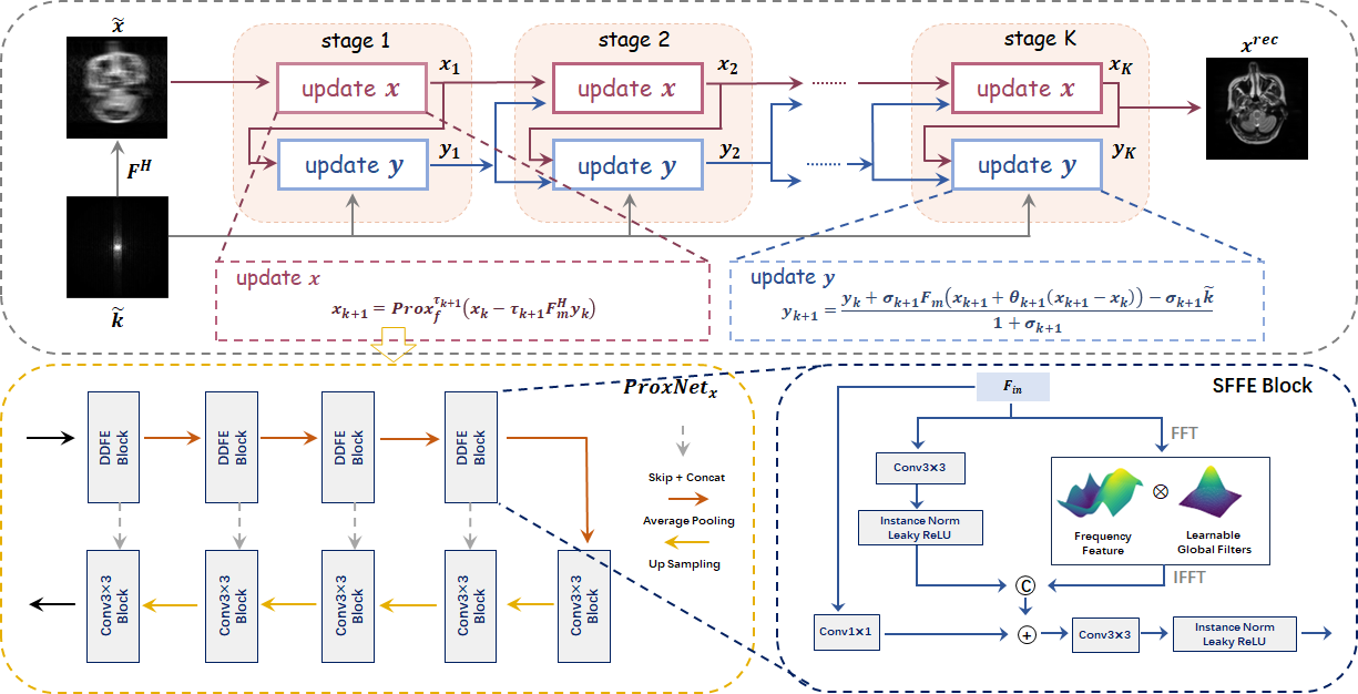
Figure 2: The overall structure of the proposed Chambolle and Pock Proximal Point Algorithm based Deep Unfolding Network (DUN-CP-PPA) is shown in the first line, which includes two parts: update $x$ module and update $y$ module. Among them, the update $y$ module is in an analytical form and is computed according to the given equation. The update $x$ module includes $\operatorname{ProxNet}_{x}$, which is shown in the second line, and extracts multi-scale features using the U-net architecture. In $\operatorname{ProxNet}_{x}$, there is a Spatial-Frequency Feature Extraction Block that captures richer feature representations.

The deep learning methods are widely used to accelerate MRI reconstruction. However, the performance of deep learning-based network heavily depends on the quantity and quality of the training data. Moreover, obtaining paired data or fully-sampled data is costly and time-consuming. To address this issue, some works adopt a self-supervised learning approach, enabling the network to train itself using only under-sampled data to learn effective image priors. However, most methods only use partial k-space data from under-sampled k-space data as input for training, resulting in a loss of valuable information.

To compensate information loss, we propose a re-visible dual-domain self-supervised learning approach as illustrated in Fig. 1. We first perform a random partition on the under-sampled k-space data $\tilde{k}$ to obtain $\tilde{k}_{p}$. Then, $\tilde{k}$ and $\tilde{k}_{p}$ are fed into the DUN-CP-PPA to obtain the corresponding reconstructed images $x^{rec}$ and $x^{rec}_{p}$. During training, we incorporate a re-visible dual-domain loss to facilitate effective learning of image priors.

In k-space, the first branch reconstructs $\tilde{k}_{p}$, which is supervised by $\tilde{k}$ through the corresponding loss function $\|F_{m}x^{rec}_{p}-\tilde{k}\|_{1}$, ensuring the model’s generative capability is effectively trained. However, after partitioning, $\tilde{k}_{p}$ loses critical information necessary for high-quality reconstruction. To address this issue, the second branch reconstructs $\tilde{k}$, ensuring that all under-sampled k-space data contribute to the training process. Inspired by [42], it is worth noting that directly utilizing $\mathcal{L}=\|F_{m}x^{rec}-\tilde{k}\|_{1}+\lambda\|F_{m}x_{p}^{rec}-\tilde{k}\|_{1}$ as the loss function may learn the identity and degrade the reconstruction performance, because $x^{rec}$ is explicitly involved in backpropagation. In order to fully utilize all k-space data while avoiding learning identity, we hope $x_{rec}$ to implicitly participate in backpropagation, allowing the model to adapt to it during the training phase. Therefore, we use the following loss function for the second branch:

$$\mathcal{L}_{k}^{rev}={\left\|\frac{F_{m}x^{rec}_{p}+\lambda F_{m}sg(x^{rec})}{1+\lambda}-\tilde{k}\right\|_{1}}.$$

In this formulation, $\text{sg}(\cdot)$ represents the stop-gradient operation, which prevents $x^{rec}$ from explicitly participating in backpropagation to avoid identity mapping issue. The parameter $\lambda$ is a hyperparameter that controls usage intensity of all k-space datad. Through this setup, $x^{rec}$ implicitly participates in training, ensuring that the model can access all under-sampled k-space data during the training process. Specifically, by incorporating this re-visible term, $x_{p}^{rec}$ is used as a transition to optimize $x^{rec}$, for the reason that $\mathcal{L}_{k}^{rev}$ tends to be large in areas where the reconstruction performance of $x^{rec}$ is poor. Consequently, the model facilitates an implicit adaptation process, from optimizing the reconstruction result $x_{p}^{rec}$, which is derived from partially under-sampled k-space data, to implicitly optimizing the reconstruction result $x^{rec}$, which is derived from all under-sampled k-space data in order to further reduce the loss. This adaptation enables the model to implicitly learn to utilize complete k-space data as input.

We combine dual-branch efforts, using $\mathcal{L}_{rev}^{k}$ to involve all under-sampled k-space data during training, thereby mitigating information loss. Additionally, we employ $\|F_{m}x^{rec}_{p}-\tilde{k}\|_{1}$ as a regularization term to ensure training stability and enhance the network’s generative capability. Therefore, we obtain the loss function for k-space as follows:

$$\mathcal{L}_{k} =\mathcal{L}_{k}^{rev}+\eta\underbrace{\|F_{m}x^{rec}_{p}-\tilde{k}\|_{1}}_{\mathcal{L}_{k}^{reg}},$$

where the first term is called the re-visible term and the second term is referred to as the regularization term. $\eta$ is a parameter that balances the regularization term and the re-visible term in k-space.

In the image domain, to improve perceptual quality and structural fidelity while leveraging the complementary information between the image domain and k-space, we define the loss function in image domain as follows:

$$\mathcal{L}_{\text{img}}= \underbrace{SSIM\left(F^{H}\frac{{F_{m}x^{rec}_{p}+\lambda F_{m}sg(x^{rec})}}{1+\lambda},F^{H}\tilde{k}\right)}_{\mathcal{L}_{\text{img}}^{rev}}$$

$$+\eta\underbrace{SSIM(F^{H}F_{m}x^{rec}_{p},F^{H}\tilde{k})}_{\mathcal{L}_{\text{img}}^{reg}},$$

where $SSIM$ denotes Structural Similarity Index Measure loss, $F^{H}$ denotes inverse fourier transform, $\lambda$ is a parameter that balances the the regularization term and the re-visible term in image domain. $\mathcal{L}_{\text{img}}^{rev}$ and $\mathcal{L}_{\text{img}}^{reg}$ in image domain correspond to the losses $\mathcal{L}_{k}^{rev}$ and $\mathcal{L}_{k}^{reg}$ in k-space, further enhancing the model’s adaptation to all available data in the image domain.

Finally, we obtain the re-visible dual-domain loss function:

$$\mathcal{L}_{d}=\mathcal{L}_{\text{img}}+\beta\mathcal{L}_{k},$$

where $\beta$ is used to balance the contributions of the loss in the k-space and image domain. During the training phase, the model has already implicitly learned to utilize all under-sampled k-space data. Therefore, during inference, we directly use all under-sampled k-space data as input to achieve better reconstruction results.

3.2 Deep Unfolding Network based on CP-PPA

To appropriately embed the MRI physics to guide reconstruction process and improve learning efficiency, we combine CP-PPA with network architecture in MRI reconstruction application. Specifically, We set the operator $L$ as the composition of the Fourier transform $F$ and the mask operation $M$, i.e., $L=F_{m}=MF$. Let $f(x)$ represent the regularization term, denoted by $R(x)$, which enforces prior constraints such as sparsity, and let $g(F_{m}x)$ denote the fidelity term, ensuring that the reconstructed image is consistent with the under-sampled k-space data. The fidelity term is defined as $g(F_{m}x)=\frac{1}{2}\|F_{m}x-\tilde{k}\|^{2}$, where $x$ represents the reconstructed image and $\tilde{k}$ represents the acquired under-sampled k-space data.

Finally, we obtain the update rules for the primal and dual variables are as follows:

$$\left\{\begin{aligned} x_{k+1}&=\operatorname{Prox}_{f}^{\tau_{k+1}}\left(x_{k}-\tau_{k+1}F_{m}^{H}y_{k}\right),\\ y_{k+1}&=\frac{y_{k}+\sigma_{k+1}F_{m}z_{k+1}-\sigma_{k+1}\tilde{k}}{1+\sigma_{k+1}}.\end{aligned}\right.$$

Through the iterative updates of $x$ and $y$, the imaging physics and image priors are incorporated. The challenge lies in how to design $\operatorname{Prox}_{f}^{\tau_{k+1}}$, as deriving it from hand-crafted regularization terms $R$ leads to slow convergence and a lack of flexibility. By combining deep unfolding techniques, we unfold this optimization algorithm into a deep unfolding network and name it DUN-CP-PPA, as shown in Fig. 2. The network structure strictly follows Eq. (3.2), using the $\operatorname{ProxNet}_{x}$ network to replace the $\operatorname{Prox}_{f}^{\tau_{k+1}}$ operator, thereby learning the priors from datasets. For $\operatorname{ProxNet}_{x}$, previous studies [9, 10] have demonstrated the effectiveness of the U-Net architecture in extracting multi-scale features and its ability to learn denoising priors. Therefore, we choose the U-Net architecture as the structure for $\operatorname{ProxNet}_{x}$. To capture both global and local feature representations and efficiently learn comprehensive image priors, we further utilize a Spatial-Frequency Feature Extraction (SFFE) Block and use residual results to enhance training stability. This can be expressed as $x_{k+1}=x_{k}+\operatorname{ProxNet}_{x}\left(x_{k}-\tau_{k+1}F_{m}^{H}y_{k}\right)$

Specifically, the $\text{ProxNet}_{x}$ architecture consists of an encoder and a decoder, as shown in Figure 2. The encoder is composed of four SFFE blocks, each containing two feature extraction branches. The input features $F_{in}$ is fed into both branches simultaneously. The first branch uses convolution, instance normalization layers, and Leaky ReLU nonlinearity to learn local features from the image domain. In the second branch, inspired by [43], the Fourier transform is applied to convert the input $x$ from the spatial domain to the frequency domain. The dot product between the learned frequency domain features and the learnable global filters is computed to enhance the global features. The inverse Fourier transform is then used to convert the learned frequency domain features back into the spatial domain. Finally, both feature representations in the spatial domain are fused using concatenation and convolution operations. A residual structure is employed to improve training stability. The decoder consists of four Conv3×3 blocks, each containing two convolutional layers with 3×3 kernels, instance normalization layers, and Leaky ReLU nonlinearity. Average pooling and transpose convolutional upsampling are employed to adjust the spatial size of the feature maps. Skip connections are utilized to enrich the feature representations.

Through $k$-stage optimization, the proposed DUN-CP-PPA is capable of accurately reconstructing the target image. For more details about the network implementation, please refer to Section 4.3. In this way, we strictly follow the algorithm for unfolding, resulting in the interpretable network DUN-CP-PPA.

By proposing DUN-CP-PPA, the imaging physics and image priors are appropriately incorporated, and the reconstruction process aligns with the iterations of the corresponding algorithm. Therefore, during the training phase, we optimize the algorithm by updating the network parameters using Eq. (3.1), ensuring that the model implicitly adapts to all under-sampled k-space data as input while preventing the model from learning the identity mapping. In the inference phase, all under-sampled k-space data can be directly input into the model, leveraging the learned reconstruction process to obtain the final reconstruction results.

Table 1: Quantitative evaluation of our method vs. other methods on the fastMRI dataset for T1 and T2 modalities under 4$\times$ and 8$\times$ acceleration with equispaced and random 1D subsampling masks. Best results among self-supervised methods are emphasized in bold. Supervised methods are marked with ^∗.

	Methods	T1 4$\times$ Acceleration		T1 8$\times$ Acceleration		T2 4$\times$ Acceleration		T2 8$\times$ Acceleration
		PSNR	SSIM	PSNR	SSIM	PSNR	SSIM	PSNR	SSIM
Equispaced	Zero-filling	27.59$\pm$0.91	0.7499$\pm$0.0285	24.29$\pm$1.23	0.6534$\pm$0.0387	26.92$\pm$1.02	0.7321$\pm$0.0279	24.36$\pm$1.11	0.6428$\pm$0.0350
	SSDU	31.79$\pm$0.95	0.8925$\pm$0.0160	27.55$\pm$0.87	0.8218$\pm$0.0194	32.42$\pm$1.20	0.9082$\pm$0.0099	25.81$\pm$0.95	0.8025$\pm$0.0207
	PARCEL	32.58$\pm$1.11	0.9010$\pm$0.0147	29.06$\pm$1.02	0.8423$\pm$0.0187	33.15$\pm$1.27	0.9102$\pm$0.0092	28.76$\pm$1.23	0.8408$\pm$0.0202
	SSMRI	35.69$\pm$1.29	0.9238$\pm$0.0121	34.76$\pm$0.93	0.9163$\pm$0.0119	33.75$\pm$1.50	0.9122$\pm$0.0119	33.12$\pm$1.28	0.9168$\pm$0.0125
	DDSS	35.05$\pm$1.17	0.9342$\pm$0.0100	34.67$\pm$0.91	0.9304$\pm$0.0091	33.88$\pm$1.20	0.9419$\pm$0.0082	33.33$\pm$1.38	0.9327$\pm$0.0106
	Noisier2Noise	36.02$\pm$1.34	0.9384$\pm$0.0104	34.87$\pm$0.93	0.9244$\pm$0.0105	34.06$\pm$1.52	0.9350$\pm$0.0122	33.49$\pm$1.42	0.9337$\pm$0.0122
	U-net∗	39.85$\pm$1.38	0.9703$\pm$0.0066	37.61$\pm$1.47	0.9579$\pm$0.0095	35.85$\pm$1.55	0.9543$\pm$0.0102	33.90$\pm$1.68	0.9396$\pm$0.0137
	Varnet∗	41.75$\pm$1.44	0.9813$\pm$0.0045	39.91$\pm$1.51	0.9740$\pm$0.0064	38.49$\pm$1.60	0.9751$\pm$0.0067	36.63$\pm$1.66	0.9658$\pm$0.0088
	Ours	39.16$\pm$1.08	0.9674$\pm$0.0058	37.35$\pm$1.39	0.9539$\pm$0.0089	36.97$\pm$1.32	0.9642$\pm$0.0070	35.17$\pm$1.52	0.9502$\pm$0.0104
Random	Zero-filling	27.41$\pm$0.92	0.7518$\pm$0.0281	24.19$\pm$1.24	0.6739$\pm$0.0371	26.77$\pm$1.02	0.7332$\pm$0.0282	24.26$\pm$1.13	0.6669$\pm$0.0345
	SSDU	34.40$\pm$1.36	0.9178$\pm$0.0134	27.66$\pm$1.32	0.8275$\pm$0.0197	32.18$\pm$1.20	0.9116$\pm$0.0119	25.38$\pm$1.03	0.7925$\pm$0.0212
	PARCEL	37.06$\pm$1.31	0.9357$\pm$0.0125	29.73$\pm$1.41	0.8456$\pm$0.0236	35.21$\pm$1.35	0.9321$\pm$0.0140	26.77$\pm$1.34	0.8073$\pm$0.0228
	SSMRI	38.49$\pm$1.58	0.9429$\pm$0.0082	30.14$\pm$2.05	0.9002$\pm$0.0143	37.67$\pm$1.56	0.9312$\pm$0.0104	31.68$\pm$1.48	0.9040$\pm$0.0124
	DDSS	40.48$\pm$1.29	0.9703$\pm$0.0055	33.09$\pm$1.36	0.9223$\pm$0.0117	36.95$\pm$1.41	0.9552$\pm$0.0083	31.33$\pm$1.44	0.9156$\pm$0.0130
	Noisier2Noise	39.55$\pm$1.45	0.9603$\pm$0.0083	30.39$\pm$1.46	0.9059$\pm$0.0128	38.58$\pm$1.55	0.9640$\pm$0.0087	31.77$\pm$1.50	0.9184$\pm$0.0145
	U-net∗	40.65$\pm$1.36	0.9723$\pm$0.0064	35.45$\pm$1.61	0.9469$\pm$0.0120	36.63$\pm$1.47	0.9570$\pm$0.0097	32.30$\pm$1.59	0.9285$\pm$0.0147
	Varnet∗	44.40$\pm$1.49	0.9873$\pm$0.0032	38.12$\pm$1.58	0.9675$\pm$0.0077	41.60$\pm$1.76	0.9842$\pm$0.0049	35.29$\pm$1.70	0.9588$\pm$0.0105
	Ours	42.56$\pm$1.39	0.9802$\pm$0.0040	34.39$\pm$1.52	0.9338$\pm$0.0118	40.03$\pm$1.58	0.9764$\pm$0.0057	32.85$\pm$1.53	0.9324$\pm$0.0130

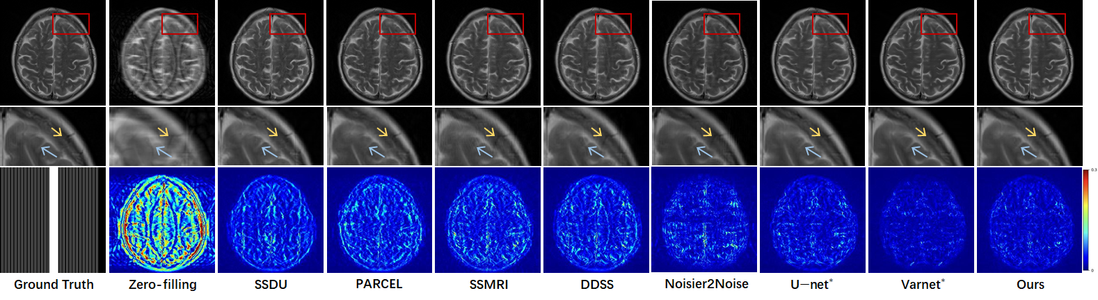
Figure 3: Visual comparison of methods for 4× acceleration using a 1D equispaced subsampling mask on fastMRI dataset. First row: Reconstructed images; second row: Zoomed region; third row: Mask and error maps.

4 Experiments

4.1 Datasets

We evaluate our method using the fastMRI dataset and the IXI dataset

fastMRI Dataset: To ensure experimental consistency, we adopt the configurations outlined in [39]. A total of 340 paired T1-weighted and T2-weighted axial brain MRI scans are selected. These are divided into three subsets: 170 volumes (comprising 2720 slice pairs) for training, 68 volumes (1088 slice pairs) for validation, and 102 volumes (1632 slice pairs) for testing. Each T1-weighted and T2-weighted image has an in-plane dimension of $320\times 320$, with a resolution of $0.68\,\text{mm}\times 0.68\,\text{mm}$ and a slice spacing of 5 mm.

IXI Dataset: The IXI dataset contains 576 paired multi-modal 3D brain MRIs, from which we select 570 pairs of PD-weighted and T2-weighted axial brain MRIs for our study. These are divided into 285 volumes for training, 115 volumes for validation, and 170 volumes for testing. Each PD-weighted and T2-weighted image has an in-plane resolution of $256\times 256$. Following the approach described in [41], we utilize the central 100 slices from each volume in our experiments.

4.2 Compared Methods

We evaluate our proposed method by comparing it with seven methods: two supervised methods (U-net, E2E-Varnet[5]) and five self-supervised methods (SSDU[31], PARCEL[44], SSMRI [15], DDSS [18], Noisier2Noise[45]). U-net consists of four encoder and four decoder to learn robust feature representations, and incorporates a data consistency block to enhance reconstruction performance. E2E-Varnet applies the variational technique, combining it with U-Net to unfold the process into an end-to-end learning framework. SSDU utilize loss defined on all the scanned data points and adopts a parallel training framework for self-supervised MRI reconstruction. PARCEL combines the advantages of contrastive representation learning with model-based deep learning MRI reconstruction models to form an efficient reconstruction strategy. SSMRI uses VarNet as its backbone and apply the diagonal weight mask to adjust loss function for better training. DDSS introduces a triple-branch, dual-domain self-supervised reconstruction approach. Noisier2Noise extends the Noisier2Noise framework, which was originally constructed for self-supervised denoising tasks, to MRI reconstruction task.

4.3 Implementation Details

In our experiments, we follow the fastMRI challenge paradigm, generating under-sampled MRIs by masking fully-sampled k-space data using Cartesian patterns. Two sampling strategies are employed: random and equispaced, at sampling ratios of 25% (4$\times$ acceleration) and 12.5% (8$\times$ acceleration). To exploit the high-energy content in low-frequency k-space, 32% of the samples are allocated to these frequencies, with the rest distributed either randomly or equispaced. For hyperparameter selection, we set the model parameters as stage$=8$, $\lambda=10$, $\eta=1$, $\beta=10$ for our experiments. All models are implemented in PyTorch and trained on a system with four NVIDIA GeForce GTX 3090 GPUs. The batch size is set to $2$, and parameters are optimized using the Adam optimizer with a learning rate of $1\times 10^{-4}$. A validation set is used to prevent overfitting and select optimal parameters, which are then applied to the test set for final evaluation. During training, the under-sampled data partitioning rate is randomly generated between $[0.2,0.8]$ which was empirically determined to provide better results. The experimental results are all based on reconstructed 3D data.

Table 2: Quantitative evaluation of our method vs. other methods on the IXI dataset for PD and T2 modalities under 4$\times$ and 8$\times$ acceleration with equispaced and random 1D subsampling masks. Best results among self-supervised methods are emphasized in bold. Supervised methods are marked with ^∗.

	Methods	PD 4$\times$ Acceleration		PD 8$\times$ Acceleration		T2 4$\times$ Acceleration		T2 8$\times$ Acceleration
		PSNR	SSIM	PSNR	SSIM	PSNR	SSIM	PSNR	SSIM
Equispaced	Zero-filling	26.96$\pm$2.45	0.6337$\pm$0.0567	24.26$\pm$2.48	0.5442$\pm$0.0700	26.56$\pm$2.04	0.6337$\pm$0.0449	24.08$\pm$2.01	0.5517$\pm$0.0535
	SSDU	35.69$\pm$1.79	0.9397$\pm$0.0072	28.47$\pm$1.78	0.8120$\pm$0.0181	34.30$\pm$1.32	0.9384$\pm$0.0094	28.27$\pm$1.84	0.8422$\pm$0.0165
	PARCEL	37.05$\pm$2.26	0.9483$\pm$0.0074	29.75$\pm$2.10	0.8378$\pm$0.0202	37.35$\pm$1.99	0.9516$\pm$0.0099	29.86$\pm$1.93	0.8531$\pm$0.0183
	SSMRI	36.96$\pm$2.40	0.9457$\pm$0.0087	31.78$\pm$2.37	0.8657$\pm$0.0206	37.07$\pm$2.06	0.9461$\pm$0.0087	31.86$\pm$2.04	0.8607$\pm$0.0223
	DDSS	39.90$\pm$2.48	0.9762$\pm$0.0069	31.08$\pm$2.39	0.8896$\pm$0.0214	38.91$\pm$2.21	0.9722$\pm$0.0072	30.44$\pm$2.08	0.8930$\pm$0.0183
	Noisier2Noise	38.78$\pm$2.40	0.9571$\pm$0.0130	31.86$\pm$2.37	0.9010$\pm$0.0222	39.12$\pm$2.14	0.9641$\pm$0.0093	32.21$\pm$2.03	0.9138$\pm$0.0165
	U-net∗	38.83$\pm$2.54	0.9715$\pm$0.0087	32.74$\pm$2.42	0.9210$\pm$0.0189	38.44$\pm$2.30	0.9694$\pm$0.0086	31.69$\pm$2.19	0.9127$\pm$0.0184
	Varnet∗	42.18$\pm$2.53	0.9866$\pm$0.0041	35.04$\pm$2.35	0.9544$\pm$0.0107	41.61$\pm$2.30	0.9854$\pm$0.0046	34.31$\pm$2.09	0.9509$\pm$0.0110
	Ours	41.64$\pm$2.46	0.9834$\pm$0.0049	33.19$\pm$2.36	0.9254$\pm$0.0164	41.36$\pm$2.20	0.9819$\pm$0.0053	33.22$\pm$2.04	0.9304$\pm$0.0142
Random	Zero-filling	26.80$\pm$2.45	0.6345$\pm$0.0595	23.99$\pm$2.48	0.5409$\pm$0.0710	26.40$\pm$2.04	0.6389$\pm$0.0470	23.83$\pm$2.01	0.5493$\pm$0.0539
	SSDU	34.99$\pm$1.75	0.9328$\pm$0.0093	28.14$\pm$1.91	0.8346$\pm$0.0172	32.78$\pm$1.60	0.9076$\pm$0.0107	27.58$\pm$1.86	0.8327$\pm$0.0168
	PARCEL	35.05$\pm$2.30	0.9344$\pm$0.0093	28.77$\pm$2.14	0.8396$\pm$0.0261	34.26$\pm$1.93	0.9167$\pm$0.0160	28.91$\pm$1.97	0.8425$\pm$0.0217
	SSMRI	35.98$\pm$2.37	0.9389$\pm$0.0092	30.36$\pm$2.38	0.8385$\pm$0.0201	34.46$\pm$2.02	0.9114$\pm$0.0120	30.66$\pm$2.02	0.8382$\pm$0.0227
	DDSS	35.43$\pm$2.41	0.9449$\pm$0.0135	29.08$\pm$2.39	0.8378$\pm$0.0290	35.38$\pm$2.10	0.9489$\pm$0.0110	28.70$\pm$2.05	0.8582$\pm$0.0225
	Noisier2Noise	36.89$\pm$2.39	0.9537$\pm$0.0128	30.52$\pm$2.38	0.8774$\pm$0.0265	35.06$\pm$2.05	0.9339$\pm$0.0146	30.78$\pm$2.01	0.8942$\pm$0.0193
	U-net∗	35.79$\pm$2.45	0.9482$\pm$0.0143	31.90$\pm$2.39	0.9080$\pm$0.0215	34.67$\pm$2.16	0.9407$\pm$0.0136	30.57$\pm$2.16	0.8945$\pm$0.0210
	Varnet∗	39.82$\pm$2.39	0.9804$\pm$0.0055	34.13$\pm$2.33	0.9465$\pm$0.0120	38.83$\pm$2.14	0.9764$\pm$0.0063	33.51$\pm$2.05	0.9433$\pm$0.0121
	Ours	38.81$\pm$2.39	0.9730$\pm$0.0072	31.37$\pm$2.33	0.9025$\pm$0.0203	38.21$\pm$2.06	0.9706$\pm$0.0072	32.17$\pm$1.97	0.9168$\pm$0.0160

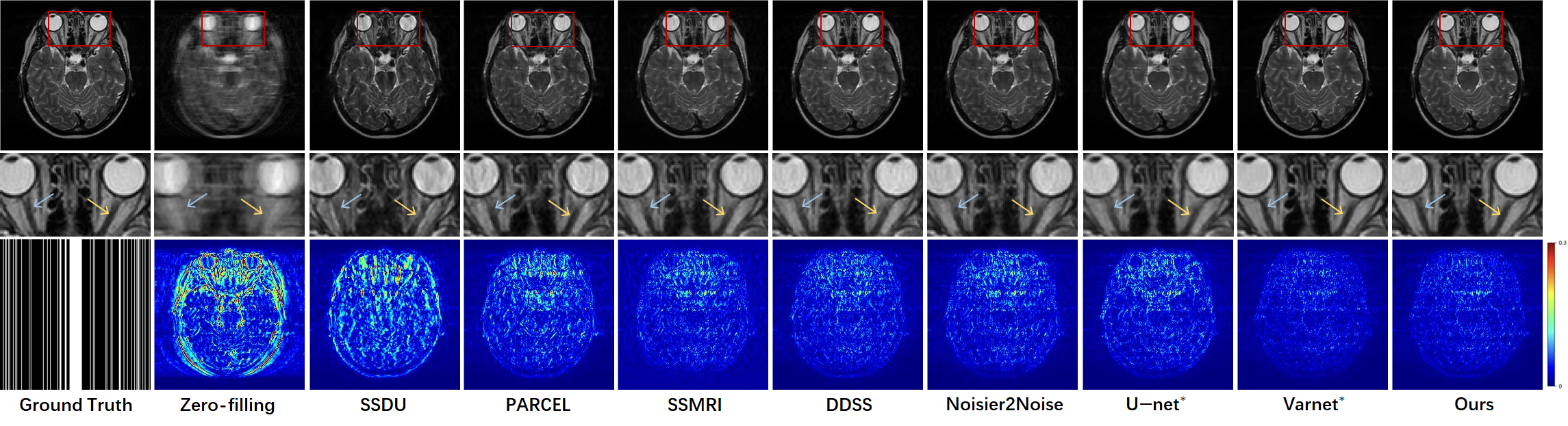
Figure 4: Visual comparison of methods for 4× acceleration using a 1D random subsampling mask on IXI dataset. First row: Reconstructed images; second row: Zoomed region; third row: Mask and error maps.

4.4 Evaluation of Proposed Method

4.4.1 Comparison with State-of-the-Arts

In Table 1, we present the quantitative comparisons in fastMRI dataset for T1- and T2-weighted image reconstructions under equispaced and random subsampling masks with 4× and 8× accelerations. The results demonstrate that our method achieves significant improvements in PSNR and SSIM compared to other self-supervised methods. Compared to supervised methods, our approach—powered by the advanced DUN-CP-PPA and a re-visible dual-domain self-supervised approach—outperforms the U-net supervised model, though there remains a performance gap when compared to the Varnet supervised model. Additionally, in Fig. 3, we provide a visual comparison of different approaches for T2-weighted images on the fastMRI dataset under equispaced subsampling with 4× acceleration. The second row highlights the zoomed-in region of interest (ROI), while the third row displays the corresponding error maps. From the close-up ROI and error maps, it is evident that our method achieves superior visual quality among all self-supervised methods, particularly for fine-grained structures, as indicated by the yellow and blue arrows.

We further validate the proposed method on the public IXI dataset. In Fig. 4 and Table 2, we report performance evaluations under 1D equispaced and random masks with 4× and 8× accelerations for both PD-weighted and T2-weighted images. Consistently, our method outperforms competing approaches qualitatively and quantitatively, aligning with the observed performance improvements on the fastMRI dataset. This indicates the strong generalizability of the proposed framework.

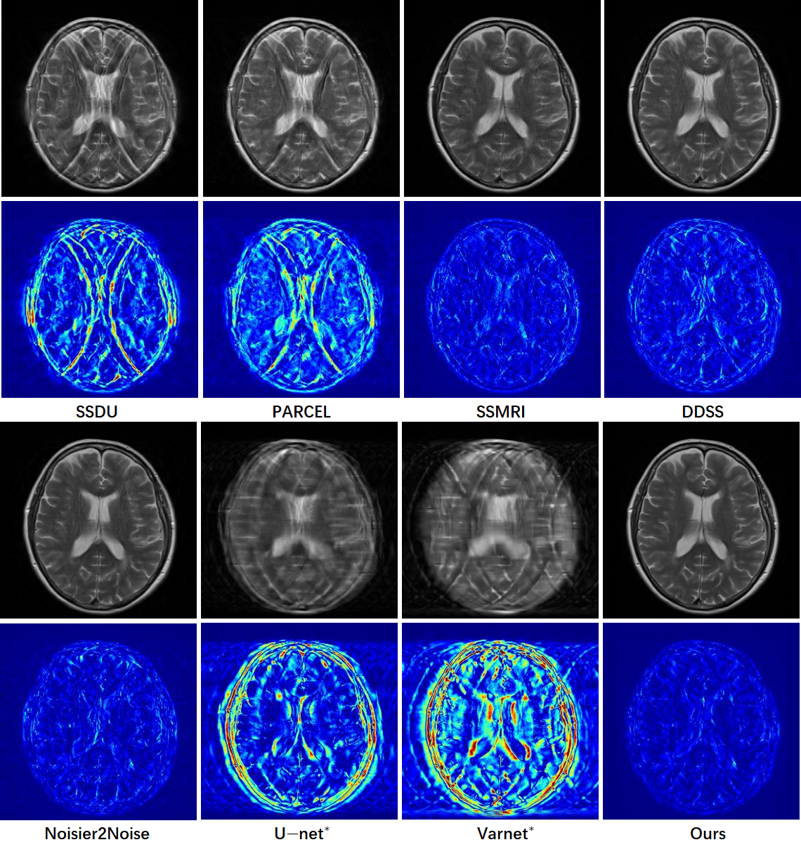
Figure 5: Visual comparison of methods for generalization performance in scenarios of pattern shift. The model is trained at 4$\times$ acceleration and tested at 8$\times$ acceleration.

4.4.2 Generalization Performance in scenarios of Pattern Shift

Generalization ability is essential for the practical application of Deep-learning based methods. To evaluate this, we design experiments to test model performance under varying sampling patterns during training and testing. Specifically, the model is trained with 4$\times$ acceleration and tested with 8$\times$ and 12$\times$ acceleration. As shown in Table 3 and Fig. 5, supervised learning methods show significant performance degradation, demonstrating their poor generalization capability to pattern shift. Self-supervised learning methods all outperform supervised methods, indicating better generalization performance to pattern shift. Among all self-supervised learning approaches, our method achieved the best results. By learning modality priors, the proposed method mitigates the Negative impact of pattern shift, resulting in superior generalization ability.

Table 3: Evaluation of Generalization Performance in scenarios of Pattern Shift.

	Loss	8$\times$ Acceleration	12$\times$ Acceleration
Equispaced	SSDU	27.48 $\pm$ 1.15	24.95 $\pm$ 1.22
		0.8543 $\pm$ 0.0178	0.7938 $\pm$ 0.0244
	PARCEL	29.19 $\pm$ 1.33	25.77 $\pm$ 1.42
		0.8591 $\pm$ 0.0195	0.7995 $\pm$ 0.0271
	SSMRI	32.32 $\pm$ 1.35	28.63 $\pm$ 1.47
		0.9154 $\pm$ 0.0132	0.8269 $\pm$ 0.0213
	DDSS	33.22 $\pm$ 1.39	29.54 $\pm$ 1.46
		0.9305 $\pm$ 0.0118	0.8911 $\pm$ 0.0169
	Noisier2Noise	32.69 $\pm$ 1.39	28.85 $\pm$ 1.48
		0.9237 $\pm$ 0.0154	0.8827 $\pm$ 0.0187
	U-net∗	24.45 $\pm$ 1.10	23.46 $\pm$ 1.12
		0.6782 $\pm$ 0.0328	0.6284 $\pm$ 0.0357
	Varnet∗	23.19 $\pm$ 1.00	22.38 $\pm$ 1.04
		0.5691 $\pm$ 0.0357	0.5173 $\pm$ 0.0380
	ours	35.31 $\pm$ 1.47	30.94 $\pm$ 1.46
		0.9535 $\pm$ 0.0094	0.9174 $\pm$ 0.0143

4.5 Ablation Analysis

4.5.1 Effect of Number of Stages

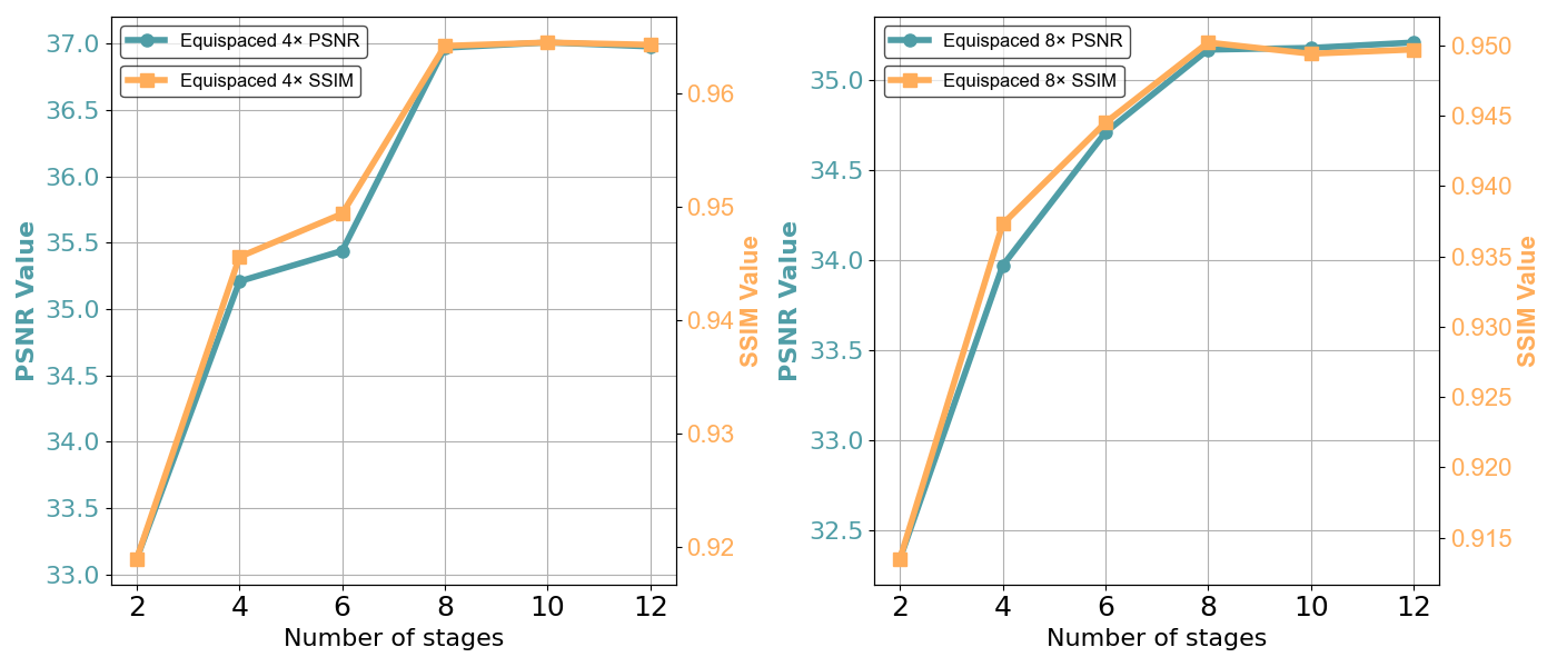
Figure 6: The PSNR and SSIM curves with different numbers of stages.

To illustrate how the number of stages $K$ influences reconstruction performance, we conduct a quantitative analysis of DUN-CP-PPA across different stage counts on four datasets, evaluating $4\times$ and $8\times$ acceleration using equispaced and random subsampling masks. As depicted in Fig. 6, the mean SSIM and PSNR values improve implicitly as $K$ increases from 2 to 8. However, after the eighth iteration, the improvements become marginal or even begin to decline. Considering both reconstruction performance and model complexity, we selected the model with $K=8$.

4.5.2 Effectiveness of DUN-CP-PPA

To evaluate the effectiveness of DUN-CP-PPA, we first replace the backbone under the same self-supervised learning approach (ours). We select HQS-Unet and VarNet as the backbones for comparison, as these are widely used in MRI reconstruction tasks. Additionally, to verify the effectiveness of the modules we proposed in DUN-CP-PPA, we conduct ablation experiments. Specifically, we replace our modules with convolution operations, naming this variant w/o SFFE. As shown in Table 4, DUN-CP-PPA achieves the best performance in all cases, and the improvement over w/o SFFE demonstrates the effectiveness of the SFFE block. Furthermore, we observe that even without the SFFE module, the deep unfolding network based on CP-PPA still outperform the deep unfolding network based on HQS.

Table 4: Comparison with different network architectures under 4× and 8× acceleration in the re-visible dual-domain self-supervised learning approach.

	BackBone	4$\times$ Acceleration	8$\times$ Acceleration
Equispaced	Varnet	34.53 $\pm$ 1.42	33.96 $\pm$ 1.49
		0.9461 $\pm$ 0.0123	0.9365 $\pm$ 0.0119
	HQS-Unet	36.05 $\pm$ 1.37	34.46 $\pm$ 1.45
		0.9571 $\pm$ 0.0085	0.9413 $\pm$ 0.0110
	w/o SFFE	36.77 $\pm$ 1.34	34.95 $\pm$ 1.51
		0.9629 $\pm$ 0.0072	0.9487 $\pm$ 0.0103
	DUN-CP-PPA	36.97$\pm$ 1.32	35.17 $\pm$ 1.48
		0.9642 $\pm$ 0.0070	0.9502 $\pm$ 0.0102

4.5.3 Effectiveness of Loss Function

To demonstrate the effectiveness of our designed re-visible dual-domain self-supervised learning approach, we conduct ablation experiments on the loss functions within six self-supervised approaches. These loss functions include:

$\mathcal{L}_{k}$, as shown in Eq. (3.1), and $\mathcal{L}_{\text{img}}$, as shown in Eq. (3.1). These two losses impose constraints in the k-space domain and the image domain, respectively.

$$\mathcal{L}_{a} =\ \|F_{m}x^{rec}-\tilde{k}\|_{1}+\beta SSIM(F^{H}F_{m}x^{rec}-F^{H}\tilde{k})$$

$$\ +\eta\|F_{m}x_{p}^{rec}-\tilde{k}\|_{1}+\beta\eta SSIM(F^{H}F_{m}x_{p}^{rec}-F^{H}\tilde{k}).$$

Eq. (4.5.3) is a dual-domain extended version of the loss $\|F_{m}x^{rec}-\tilde{k}\|_{1}+\eta\|F_{m}x_{p}^{rec}-\tilde{k}\|_{1}$. It is used to verify that this formulation is suboptimal compared to our proposed loss function.

$\mathcal{L}_{reg}=\mathcal{L}_{k}^{reg}+\mathcal{L}_{\text{img}}^{reg}$: the proposed regularized term, a dual-domain extended version of the loss $\mathcal{L}_{k}^{reg}$ aimed at improving performance and ensuring a fair comparison.

$\mathcal{L}_{rev}=\mathcal{L}_{k}^{rev}+\mathcal{L}_{\text{img}}^{rev}$: the proposed re-visible term, which can ensure that all under-sampled k-space data participate in the training process as well, enabling the model to adapt to all k-space data as input.

$\mathcal{L}_{d}=\mathcal{L}_{\text{img}}+\beta\mathcal{L}_{k}$: our proposed loss function, which combines revisible dual-domain supervision and implicitly involves $x_{p}^{rec}$ in the training.

Table 5: Performance comparison of different loss functions.

	Loss	4$\times$ Acceleration	8$\times$ Acceleration
Equispaced	$\mathcal{L}_{k}$	35.40 $\pm$ 1.55	34.07 $\pm$ 1.34
		0.9485 $\pm$ 0.0104	0.8948 $\pm$ 0.0188
	$\mathcal{L}_{\text{img}}$	35.82 $\pm$ 1.39	34.64 $\pm$ 1.52
		0.9468 $\pm$ 0.0098	0.9410 $\pm$ 0.0118
	$\mathcal{L}_{a}$	35.89 $\pm$ 1.32	34.70 $\pm$ 1.53
		0.9605 $\pm$ 0.0076	0.9478 $\pm$ 0.0102
	$\mathcal{L}_{reg}$	36.19 $\pm$ 1.43	34.56 $\pm$ 1.51
		0.9614 $\pm$ 0.0082	0.9451 $\pm$ 0.0106
	$\mathcal{L}_{rev}$	36.76 $\pm$ 1.38	34.90 $\pm$ 1.52
		0.9628 $\pm$ 0.0073	0.9484 $\pm$ 0.0104
	$\mathcal{L}_{d}$	36.97$\pm$ 1.32	35.17 $\pm$ 1.48
		0.9642 $\pm$ 0.0070	0.9502 $\pm$ 0.0102

As shown in Table 5, the experiments demonstrate that the dual-domain loss outperforms the single-domain loss, reflecting the complementary information between the two domains. Loss functions $\mathcal{L}_{a}$ involving all k-space data in training, however, perform worse in Equispaced $4\times$ Acceleration than those involving only partial k-space data, indicating that the way $\mathcal{L}_{a}$ involves all k-space data in training is suboptimal compared to our proposed $\mathcal{L}_{d}$, which shows a significant improvement over $\mathcal{L}_{\text{reg}}$. $\mathcal{L}_{d}$ performs better than $\mathcal{L}_{a}$, and $\mathcal{L}_{\text{rev}}$ outperforms $\mathcal{L}_{\text{reg}}$, both confirming the effectiveness of the re-visible terms.

4.5.4 Evaluation of Hyper-Parameter

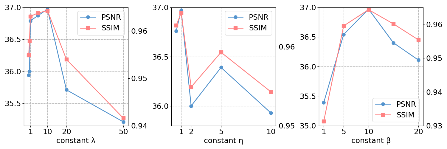
Figure 7: Impact of hyper-parameters $\lambda$, $\eta$, and $\beta$ on PSNR and SSIM. The figure shows how different values of these hyper-parameters affect the quality of reconstructed images, with metrics including PSNR (in blue) and SSIM (in red).

In this section, we evaluate the impact of hyperparameters in the loss function on the reconstruction performance and present the results in Fig. 7. Specifically, the hyperparameter $\beta$ is used to balance the loss functions in both the image domain and k-space, while $\eta$ controls the balance between the re-visible and regularization terms, which helps to stabilize the training process. The hyperparameter $\lambda$ control the contribution of all k-space data as input during training. As shown in the figure 7, the different values of these hyperparameters significantly affect the quality of the reconstructed images, as measured by the PSNR and SSIM. We set $\lambda\in\{0.1,0.5,1,10,20,50\}$; $\eta\in\{1,2,5,10\}$; $\beta\in\{1,5,10,20\}$ for the experiments. Based on the observed trends, we select $\beta=10$, $\eta=1$, and $\lambda=10$ as the optimal hyperparameter values to achieve the best reconstruction results.

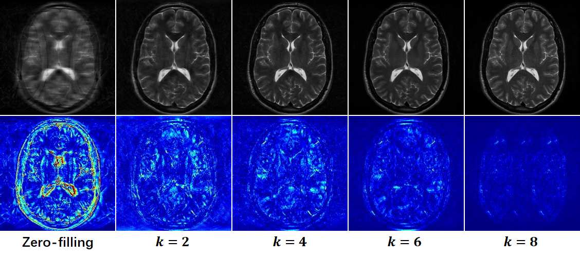
Figure 8: Visualization of reconstruction results at different stages $k$.

4.5.5 Model Verification

In this section, we conduct a model verification experiment to demonstrate the reconstruction results of the proposed DUN-CP-PPA under different stages. As shown in Fig. 8, it is evident that as the number of stages $k$ increases, the image quality improves. These results validate the design of our optimization-inspired iterative network, and the re-visible dual-domain self-supervised learning framework enables the proposed DUN-CP-PPA to achieve the expected MRI reconstruction. Furthermore, our network demonstrates superior transparency compared to other methods.

5 Conclusion

This paper proposes a re-visible dual-domain self-supervised deep unfolding network to significantly enhance reconstruction performance using only under-sampled k-space data for training. Specifically, we design a re-visible dual-domain self-supervised learning framework and introduce a re-visible dual-domain loss function to reduce information loss caused by further partitioning during training, enabling the model to efficiently adapt to all under-sampled k-space data. Furthermore, by unfolding each stage of CP-PPA into dedicated network modules, we incorporate imaging physics and image priors into the reconstruction process, resulting in the DUN-CP-PPA. To further enhance the ability of DUN-CP-PPA to learn comprehensive image priors, we integrate the SFFE module. Extensive experiments on the fastMRI and IXI datasets demonstrate that our method significantly outperforms existing approaches.

References

References

- [1] M. Lustig, D. Donoho, and J. M. Pauly, “Sparse MRI: the application of compressed sensing for rapid MR imaging,” Magn. Reson. Med., vol. 58, no. 6, pp. 1182–1195, Dec. 2007. PMID: 17969013.
- [2] Z. Lai, X. Qu, Y. Liu, D. Guo, J. Ye, Z. Zhan, and Z. Chen, “Image reconstruction of compressed sensing MRI using graph-based redundant wavelet transform,” Med. Image Anal., vol. 27, pp. 93–104, Jan. 2016. PMID: 26096982.
- [3] Y. Yang, F. Liu, W. Xu, and S. Crozier, “Compressed sensing MRI via two-stage reconstruction,” IEEE Trans. Biomed. Eng., vol. 62, no. 1, pp. 110–118, Jan. 2015. PMID: 25069108.
- [4] M. Ender and E. Eksioglu, “Decoupled algorithm for MRI reconstruction using nonlocal block matching model: BM3D-MRI,” J. Math. Imaging Vis., vol. 56, no. 3, pp. 430–440, Nov. 2016.
- [5] A. Sriram et al., “End-to-end variational networks for accelerated MRI reconstruction,” in Medical Image Computing and Computer-Assisted Intervention – MICCAI 2020, A. L. Martel et al., Eds., Lecture Notes in Computer Science, vol. 12262, Cham: Springer, 2020, pp. 64–73.
- [6] G. Yang et al., “DAGAN: deep de-aliasing generative adversarial networks for fast compressed sensing MRI reconstruction,” IEEE Trans. Med. Imaging, vol. 37, no. 6, pp. 1310–1321, June 2018.
- [7] J. Jiang, J. Chen, H. Xu, Y. Feng, and J. Zheng, “GA-HQS: MRI reconstruction via a generically accelerated unfolding approach,” in Proc. 2023 IEEE Int. Conf. Multimedia Expo (ICME), Brisbane, Australia, 2023, pp. 186–191.
- [8] J. Jiang, Y. Feng, J. Chen, D. Guo, and J. Zheng, “Latent-space unfolding for MRI reconstruction,” in Proc. 31st ACM Int. Conf. Multimedia (MM ’23), Ottawa, ON, Canada, 2023, pp. 1294–1302.
- [9] B. Xin, T. Phan, L. Axel, and D. Metaxas, “Learned half-quadratic splitting network for MR image reconstruction,” in Proc. 5th Int. Conf. Med. Imaging with Deep Learning (MIDL), vol. 172, E. Konukoglu et al., Eds., PMLR, Jul. 2022, pp. 1403–1412.
- [10] Y. Yang, J. Sun, H. Li, and Z. Xu, “ADMM-CSNet: a deep learning approach for image compressive sensing,” IEEE Trans. Pattern Anal. Mach. Intell., vol. 42, no. 3, pp. 521–538, Mar. 1, 2020.
- [11] Y. Yang, N. Wang, H. Yang, J. Sun, and Z. Xu, “Model-driven deep attention network for ultra-fast compressive sensing MRI guided by cross-contrast MR image,” in Medical Image Computing and Computer-Assisted Intervention – MICCAI 2020, A. L. Martel et al., Eds., Lecture Notes in Computer Science, vol. 12262, Cham: Springer, 2020, pp. 188–198.
- [12] J. Jiang, Z. He, Y. Quan, J. Wu, and J. Zheng, “PGIUN: physics-guided implicit unrolling network for accelerated MRI,” IEEE Trans. Comput. Imaging, vol. 10, pp. 1055–1068, 2024.
- [13] P. Huang, C. Zhang, X. Zhang, X. Li, L. Dong, and L. Ying, “Self-supervised deep unrolled reconstruction using regularization by denoising,” IEEE Trans. Med. Imaging, vol. 43, no. 3, pp. 1203–1213, Mar. 2024.
- [14] B. Zhou et al., “DSFormer: A dual-domain self-supervised transformer for accelerated multi-contrast MRI reconstruction,” in Proc. IEEE/CVF Winter Conf. Applications of Computer Vision (WACV), 2023, pp. 4955–4964.
- [15] T. Klug, D. Atik, and R. Heckel, “Analyzing the sample complexity of self-supervised image reconstruction methods,” in Adv. Neural Inf. Process. Syst., vol. 36, 2024.
- [16] Y. Yan et al., “DC-SiamNet: deep contrastive siamese network for self-supervised MRI reconstruction,” Comput. Biol. Med., vol. 167, Art. no. 107619, 2023.
- [17] Z. X. Cui et al., “Self-score: self-supervised learning on score-based models for MRI reconstruction,” arXiv preprint arXiv:2209.00835, 2022.
- [18] B. Zhou et al., “Dual-domain self-supervised learning for accelerated non-Cartesian MRI reconstruction,” Med. Image Anal., vol. 81, Art. no. 102538, 2022.
- [19] Q. Wang, Z. Wen, J. Shi, Q. Wang, D. Shen, and S. Ying, “Spatial and modal optimal transport for fast cross-modal MRI reconstruction,” IEEE Trans. Med. Imaging, vol. 43, no. 11, pp. 3924–3935, Nov. 2024.
- [20] H. Zhang, Q. Wang, J. Shi, S. Ying, and Z. Wen, “Deep unfolding network with spatial alignment for multi-modal MRI reconstruction,” Med. Image Anal., vol. 99, Art. no. 103331, 2025.
- [21] W. Gan et al., “Self-supervised deep equilibrium models With theoretical guarantees and applications to MRI reconstruction,” IEEE Trans. Comput. Imaging, vol. 9, pp. 796–807, 2023.
- [22] Y. Korkmaz, T. Cukur, and V. M. Patel, “Self-supervised MRI reconstruction with unrolled diffusion models,” in Medical Image Computing and Computer-Assisted Intervention – MICCAI 2023, H. Greenspan et al., Eds., Lecture Notes in Computer Science, vol. 14229, Cham: Springer, 2023, pp. 515–526.
- [23] B. Yaman, S. A. H. Hosseini, S. Moeller, J. Ellermann, K. Uğurbil, and M. Akçakaya, “Self‐supervised learning of physics‐guided reconstruction neural networks without fully sampled reference data,” Magn. Reson. Med., vol. 84, no. 6, pp. 3172–3191, Dec. 2020.
- [24] Z. Guo and H. Gan, “CPP-Net: embracing multi-scale features fusion into deep unfolding CP-PPA network for compressive sensing,” in Proc. IEEE/CVF Conf. Comput. Vis. Pattern Recognit. (CVPR), June 2024, pp. 25086–25095.
- [25] S. Liang, A. Sreevatsa, A. Lahiri, and S. Ravishankar, “LONDN-MRI: Adaptive local neighborhood-based networks for MR image reconstruction from under-sampled data,” in Proc. 2022 IEEE 19th Int. Symp. Biomed. Imaging (ISBI), Kolkata, India, 2022, pp. 1–4.
- [26] A. Chambolle and T. Pock, “A first-order primal-dual algorithm for convex problems with applications to imaging,” J. Math. Imaging Vis., vol. 40, pp. 120–145, May 2011.
- [27] G. Gu, B. He, and X. Yuan, “customized proximal point algorithms for linearly constrained convex minimization and saddle-point problems: a unified approach,” Comput. Optim. Appl., vol. 59, pp. 135–161, Oct. 2014.
- [28] B. He and X. Yuan, “Convergence analysis of primal-dual algorithms for a saddle-point problem: from contraction perspective,” SIAM J. Imaging Sci., vol. 5, no. 1, pp. 119–149, 2012.
- [29] M. Zhu and T. Chan, “An efficient primal-dual hybrid gradient algorithm for total variation image restoration,” UCLA CAM Report, vol. 34, pp. 8–34, 2008.
- [30] A. Beck and M. Teboulle, “A fast iterative shrinkage-thresholding algorithm for linear inverse problems,” SIAM J. Imaging Sci., vol. 2, no. 1, pp. 183–202, 2009.
- [31] C. Hu, C. Li, H. Wang, Q. Liu, H. Zheng, and S. Wang, “Self-supervised learning for MRI reconstruction with a parallel network training framework,” in Medical Image Computing and Computer-Assisted Intervention – MICCAI 2021, M. de Bruijne et al., Eds., Lecture Notes in Computer Science, vol. 12906, Cham: Springer, 2021, pp. 393–402.
- [32] M. A. Griswold, P. M. Jakob, R. M. Heidemann, M. Nittka, V. Jellus, J. Wang, B. Kiefer, and A. Haase, “Generalized autocalibrating partially parallel acquisitions (GRAPPA),” Magn. Reson. Med., vol. 47, pp. 1202–1210, 2002.
- [33] M. Lustig and J. M. Pauly, “SPIRiT: iterative self-consistent parallel imaging reconstruction from arbitrary k-space,” Magn. Reson. Med., vol. 64, pp. 457–471, 2010.
- [34] M. Akçakaya, S. Moeller, S. Weingärtner, and K. Uğurbil, “Scan-specific robust artificial-neural-networks for k-space interpolation (RAKI) reconstruction: database-dree deep learning for fast imaging,” Magn. Reson. Med., vol. 81, pp. 439–453, 2019.
- [35] T. H. Kim, P. Garg, and J. P. Haldar, “LORAKI: autocalibrated recurrent neural networks for autoregressive MRI reconstruction in k-space,” arXiv preprint arXiv:1904.09390, 2019.
- [36] K. Krupa and M. Bekiesińska-Figatowska, “Artifacts in magnetic resonance imaging,” Pol. J. Radiol., vol. 80, pp. 93–106, Feb. 2015. PMID: 25745524; PMCID: PMC4340093.
- [37] X. Meng, K. Sun, J. Xu, X. He, and D. Shen, “Multi-modal modality-masked diffusion network for brain MRI synthesis with random modality missing,” IEEE Trans. Med. Imaging, vol. 43, no. 7, pp. 2587–2598, July 2024.
- [38] C.-M. Feng et al., “Multimodal transformer for accelerated MR imaging,” IEEE Trans. Med. Imaging, vol. 42, no. 10, pp. 2804–2816, Oct. 2023.
- [39] K. Xuan et al., “Multimodal MRI reconstruction assisted with spatial alignment network,” IEEE Trans. Med. Imaging, vol. 41, no. 9, pp. 2499–2509, Sept. 2022.
- [40] P. Lei, F. Fang, G. Zhang, and T. Zeng, “Decomposition-based variational network for multi-contrast MRI super-resolution and reconstruction,” in Proc. IEEE/CVF Int. Conf. Comput. Vis. (ICCV), Oct. 2023, pp. 21296–21306.
- [41] P. Lei, F. Fang, G. Zhang, and M. Xu, “Deep unfolding convolutional dictionary model for multi-contrast MRI super-resolution and reconstruction,” in Proc. 32nd Int. Joint Conf. Artif. Intell. (IJCAI), E. Elkind, Ed., Int. Joint Conf. Artif. Intell. Organization, 2023, pp. 1008–1016.
- [42] Z. Wang, J. Liu, G. Li, and H. Han, “Blind2Unblind: self-supervised image denoising with visible blind spots,” in Proc. IEEE/CVF Conf. Comput. Vis. Pattern Recognit. (CVPR), New Orleans, LA, USA, Jun. 2022, pp. 2027–2036.
- [43] Y. Rao, W. Zhao, Z. Zhu, et al., “Global filter networks for image classification,” in Advances in Neural Information Processing Systems (NeurIPS), 2021, vol. 34, pp. 980–993.
- [44] S. Wang, R. Wu, C. Li, et al., “Parcel: physics-based unsupervised contrastive representation learning for multi-coil MR imaging,” in IEEE/ACM Transactions on Computational Biology and Bioinformatics, 2022, vol. 20, no. 5, pp. 2659–2670.
- [45] C. Millard and M. Chiew, “A theoretical framework for self-supervised MR image reconstruction using sub-sampling via variable density Noisier2Noise,” in IEEE Transactions on Computational Imaging, 2023.
- [46] Z. Li, S. Li, Z. Zhang, et al., “Radial undersampled MRI reconstruction using deep learning with mutual constraints between real and imaginary components of K-space,” IEEE J. Biomed. Health Inform., 2024.
- [47] Z. Wu and X. Li, “Adaptive knowledge distillation for high-quality unsupervised MRI reconstruction with model-driven priors,” IEEE J. Biomed. Health Inform., 2024.
- [48] X. Sun, Y. Pang, Y. Liu, et al., “Multi-modal multi-slice cooperative dual-domain cascaded de-aliasing network for MR imaging reconstruction,” IEEE J. Biomed. Health Inform., 2024.
- [49] Y. Luo, M. Wei, S. Li, et al., “An effective co-support guided analysis model for multi-contrast MRI reconstruction,” IEEE J. Biomed. Health Inform., vol. 27, no. 5, pp. 2477–2488, 2023.