Stabilization of Strictly Pre-Dissipative Receding Horizon Linear Quadratic Control by Terminal Costs

Abstract

Asymptotic stability in receding horizon control is obtained under a strict pre-dissipativity assumption, in the presence of suitable state constraints. In this paper we analyze how terminal constraints can be replaced by suitable terminal costs. We restrict to the linear-quadratic setting as that allows us to obtain stronger results, while we analyze the full nonlinear case in a separate contribution.

I Introduction

Receding horizon control (often used synonymously with model predictive control) is a control technique in which a finite horizon optimal control problem is solved in each time step and only the first element of the resulting optimal control sequence is used, while in the next time step the state is measured and the problem solved again to update the control [1, 2]. Under suitable stabilizability and regularity conditions, this scheme yields a practically asymptotically stable closed loop if the system is strictly dissipative with supply function defined via the stage cost of the finite horizon optimal control problem [2, Chapter 8]. In this case, we call the optimal control problem strictly dissipative. Here, the size of the “practical” neighborhood of the equilibrium to which the closed-loop solution converges is determined by the length of the finite optimization horizon. True (as opposed to practical) asymptotic stability can be achieved by using suitable terminal constraints and costs, see [3, 4] or Theorem 8.13 in [2]. In these approaches the terminal cost is typically a local control Lyapunov function for the system and the terminal constraints are needed because the design of a global control Lyapunov function is usually a very difficult task. As a simpler alternative, it was shown in [5] that linear terminal costs can also be used to obtain true asymptotic stability.

The strict dissipativity property that is at the heart of all these results requires the existence of a so-called storage function $\lambda$ mapping the state space into the reals. It is a strengthened version of the system theoretic dissipativity property introduced by Willems in his seminal papers [6, 7] and also featured in his slightly earlier paper [8] on linear quadratic optimal control and the algebraic Riccati equation. Readers familiar with Lyapunov’s stability theory can see the storage function $\lambda$ as a generalization of a Lyapunov function. However, unlike Lyapunov functions, $\lambda$ need not attain nonnegative values. However, it must be bounded from below, and this property is crucial for deriving the (practical) stability properties for receding horizon control cited above.

For generalized linear quadratic problems (by which we mean problems with linear dynamics and a cost function containing quadratic and linear terms) with state space $\mathbb{R}^{n_{x}}$, a standard construction for a storage function results in a function of the form $\lambda(x)=x^{T}Px+\nu^{T}x$, for $P\in\mathbb{R}^{n_{x}\times n_{x}}$ and $\nu\in\mathbb{R}^{n_{x}}$, see [9, Proposition 4.5]. Clearly, such a function $\lambda$ is in general not bounded from below and Example 2.3 in [9], which we also present as Example II.1, below, shows that storage functions unbounded from below may occur even for very simple scalar problems. While the potential unboundedness of $\lambda$ has been handled somewhat informally in [9], later in [10] the variant of strict dissipativity with storage function not bounded from below has been termed strict pre-dissipativity. For strictly pre-dissipative problems, one way to restore strict dissipativity and thus (practical) asymptotic stability is to suitably restrict the state space by means of state constraints, e.g., to a compact set, on which $\lambda$ is bounded from below.

Since such a restriction of the state space may not always be desirable, in this paper we will look at an alternative way to regain (practical) asymptotic stability. More precisely, we want to answer the following question: Given a receding horizon control scheme with strictly pre-dissipative optimal control problem, can we add a simple terminal cost that guarantees (practical) asymptotic stability? Here “simple” means that we don’t want to design control Lyapunov function terminal costs but terms that are easier to compute. Thus, the answer we are looking for is conceptually similar to the one given in [5], but instead of the linear terminal cost from this reference we will see that a quadratic terminal cost is the right object here. We emphasize that no terminal constraints are needed in this approach. While we consider the general nonlinear case in the companion paper [11], in this paper we focus on the linear-quadratic case, for which we are able to provide stronger results, which we also connect to the generic results for the nonlinear case.

The analysis in this paper will deal with linear quadratic problems. After delivering the main results, we will briefly comment on the connections with the general nonlinear case. For this linear-quadratic problems, the question about asymptotic stability is closely linked with the existence of particular solutions to algebraic Riccati equations. Hence, we will make ample use of results from this area. The remainder of this paper is organized as follows. In Section II we introduce the problem and provide some definitions. We provide preliminary results in Section III, which are instrumental for our main results, delivered in Section IV. We discuss the connections with other results available in the literature in Section V. We illustrate our theory with a numerical example in section VI and we draw our conclusions in Section VII.

II Problem Statement

We consider discrete-time systems of the form

$$x_{k+1}=Ax_{k}+Bu_{k},$$ (1)

where $x\in\mathbb{R}^{n_{x}}$ and $u\in\mathbb{R}^{n_{u}}$ denote the states and controls respectively.

Model predictive control consists in minimizing a given stage cost $\ell:\mathbb{R}^{n_{x}}\times\mathbb{R}^{n_{u}}\to\mathbb{R}$ over a given finite prediction horizon $N$, possibly subject to constraints and with the addition of a terminal cost. The receding horizon optimal control problem (RH-OCP) reads

$$\min_{x_{0},u_{0},\ldots,x_{N}}\ \ \sum_{k=0}^{N-1}\ell(x_{k},u_{k})+V^{\mathrm{f}}(x_{N})$$ (2a)

$$\mathrm{s.t.}\ \ x_{0}=\hat{x}_{j},$$ (2b)

$$x_{k+1}=Ax_{k}+Bu_{k}, k\in\mathbb{I}_{0}^{N-1},$$ (2c)

$$Cx_{k}+Du_{k}\leq 0, k\in\mathbb{I}_{0}^{N-1},$$ (2d)

where $h:\mathbb{R}^{n_{x}}\times\mathbb{R}^{n_{u}}\to\mathbb{R}^{l}$ defines the state and input constraints and inequality (2d) is to be understood componentwise.

While we study the nonlinear case in the companion paper [11], in this paper we focus on the linear-quadratic case, i.e.,

$$\ell(x,u) =\left[\begin{array}[]{c}x\\ u\end{array}\right]^{\top}H\left[\begin{array}[]{c}x\\ u\end{array}\right],$$ (3e)

$$V^{f}(x) =x^{\top}P^{\mathrm{f}}x.$$ (3f)

Note that, as the case of additional constant terms in (1) and additional linear terms in (3e)-(3f) has been fully analyzed in [5], in this section we assume for simplicity that these quantities are zero.

Starting in the initial value $\hat{x}_{0}$ at time instant $j=0$, at every time instant $j\geq 0$ the state $\hat{x}_{j}$ is measured, Problem (2) is solved, and the first optimal input $u_{0}^{\star}$ is applied to the system to obtain

$$\hat{x}_{j+1}=A\hat{x}_{j}+Bu_{0}^{\star}.$$ (4)

This procedure is repeated iteratively for all $j\geq 0$.

In this paper, we are interested in obtaining stability properties of the closed loop system (4). While stability results are abundant for the case of suitably formulated terminal constraints and Lyapunov function terminal costs [12, 13, 14, 15, 16], we focus next on the case of no terminal constraint. This case has been analyzed, e.g., in [17, 5, 18, 19], where we can further distinguish between formulations without terminal cost and formulations with simple terminal costs that need not be Lyapunov functions, which are usually difficult to design. This last approach has in particular been taken in [17, 5] by using a linear terminal cost and the present paper can be seen as a continuation of this research. As in these references, our analysis is based on dissipativity concepts.

We define the infinite-horizon Optimal Control Problem (OCP) related to (3), known as the Linear Quadratic Regulator (LQR), as

$$V(x_{0})=\min_{u_{0},u_{1},\ldots}\ \lim_{N\to\infty}\sum_{k=0}^{N-1}\ell(x_{k},u_{k})+x_{N}^{\top}P^{\mathrm{f}}x_{N}$$ (5a)

$$\mathrm{s.t.}\ \ x_{k+1}=Ax_{k}+Bu_{k}.$$ (5b)

Under suitable assumptions, the LQR solution is characterized by a solution $P$ with associated $K$ of the Discrete Algebraic Riccati Equation (DARE)

$$P =Q+A^{\top}PA-(S^{\top}+A^{\top}PB)K,$$ (6a)

$$K =(R+B^{\top}PB)^{-1}(S+B^{\top}PA),$$ (6b)

which provides both the optimal feedback law

$$F(x)=-Kx,$$

defining the optimal control via $u_{k}^{\star}=-Kx_{k}^{\star}$, and the associated quadratic value function

$$V(x)=x^{\top}Px.$$

For a finite horizon $N$, the cost-to-go and the optimal feedback law are in this case time-varying and read respectively $V_{k}(x)=x^{\top}P_{N-k}x$, and $F_{k}(x)=-K_{N-k}x$, where

$$P_{n+1} =Q+A^{\top}P_{n}A-(S^{\top}+A^{\top}P_{n}B)K_{n+1},$$ (7a)

$$K_{n+1} =(R+B^{\top}P_{n}B)^{-1}(S+B^{\top}P_{n}A),$$ (7b)

defines $P_{1},\ldots,P_{N}$ and $K_{0},\ldots,K_{N}$ inductively with $P_{0}=P^{\mathrm{f}}$. Note that for an RH-OCP with data of the linear quadratic form (3) the receding horizon control in (4) is given by

$$u_{0}^{\star}=-K_{N}(\hat{x}_{j}).$$

In the context of this paper, it is paramount to clarify the fact that matrix $P$ defining the optimal value function of the infinite-horizon LQR problem and the (symmetric) solutions $P$ of the DARE do not necessarily coincide, as we explain next. It is well-known that the DARE has in general infinitely many symmetric solutions [8, 20, 21, 22], which can be interpreted as solutions of different OCPs. Note that the DARE might also have non-symmetric solutions, but these are not relevant in the context of this paper. Therefore, whenever referring to a solution of the DARE we will implicitly restrict to the set of symmetric solutions.

We call a solution $P_{\mathrm{s}}$ with associated $K_{\mathrm{s}}$ stabilizing, if all eigenvalues $\mu$ of $A-BK_{\mathrm{s}}$ satisfy $|\mu|<1$, i.e., if $A-BK_{\mathrm{s}}$ is Schur stable. If there exists a stabilizing solution to the DARE, then it is unique, i.e., all other solutions are not stabilizing [21, 22]. Unfortunately, even in case the DARE does have a stabilizing solution, this one need not be the solution to the LQR, as proven by the next example.

Example II.1

Consider an LQR problem defined by $A=2$, $B=1$, $Q=0$, $S=0$, $R=1$, and $P^{\mathrm{f}}=0$. The DARE reads

$$P=4P-\frac{4P^{2}}{1+P}, K=\frac{2P}{1+P},$$

and has the two solutions

$$P=\{0,3\}, K=\{0,1.5\}.$$

Both solutions of the DARE correspond to the solution of an OCP. The first one is

$$\min_{u_{0},u_{1},\ldots}\ \sum_{k=0}^{\infty}u_{k}^{2}$$

$$\mathrm{s.t.}\ \ x_{k+1}=Ax_{k}+Bu_{k}, k\in\mathbb{I}_{0}^{\infty},$$

which has the trivial solution $u_{k}^{\star}=0$, for all $k$ and corresponds to $P=0$, $K=0$, which does not stabilize the system. The second OCP is

$$\min_{u_{0},u_{1},\ldots}\ \sum_{k=0}^{\infty}u_{k}^{2}$$

$$\mathrm{s.t.}\ \ x_{k+1}=Ax_{k}+Bu_{k}, k\in\mathbb{I}_{0}^{\infty},$$

$$\lim_{k\to\infty}x_{k}=0,$$

which corresponds to the stabilizing solution $P=3$ and $K=1.5$. Thus, the asymptotic state constraint $\lim_{k\to\infty}x_{k}=0$ leads to a stabilizing optimal solution.

Note that for this system, the storage function $\lambda(x)=-x^{2}$ yields the rotated cost matrix

$$\bar{H}=\left[\begin{array}[]{ll}3&2\\ 2&2\end{array}\right]\succ 0,$$

whose positive definiteness confirms that strict pre-dissipativity holds. Yet, asymptotic stability cannot be achieved unless suitable constraints are introduced. As already mentioned, we will prove in this paper that the constraints can be replaced by a suitably defined quadratic terminal cost. In the case of this example, one can see that any terminal cost $V^{f}(x)=x^{\top}P^{\mathrm{f}}x$ with $P^{\mathrm{f}}>0$ yields asymptotic stability. $\hfill\square$

III Preliminary Results

In this section we provide some useful results that we will exploit in order to prove our main contributions.

III-A Cost Rotation and Pre-Stabilization

In order to derive our results, let us provide a few useful facts next.

Strict $(x,u)$-Pre-Dissipativity and Rotated Cost

For a given matrix $\Lambda$ and storage function $\lambda(x)=x^{\top}\Lambda x$, we define the rotated cost

$$L(x,u):=\left[\begin{array}[]{c}x\\ u\end{array}\right]^{\top}H_{\Lambda}\left[\begin{array}[]{c}x\\ u\end{array}\right],$$ (8e)

with

$$H_{\Lambda} :=\left[\begin{array}[]{ll}Q+\Lambda-A^{\top}\Lambda A&S^{\top}-A^{\top}\Lambda B\\ S-B^{\top}\Lambda A&R-B^{\top}\Lambda B\end{array}\right].$$ (8h)

Definition III.1 (Quadratic Strict $(x,u)$-Pre-Dissipativity)

Quadratic strict $(x,u)$-pre-dissipativity holds if there exists a scalar $\epsilon>0$ such that

$$L(x,u)\geq\epsilon(\|x\|^{2}+\|u\|^{2}), H_{\Lambda}\succ 0.$$ or, equivalently, (9)

It has been proven in [10, Lemma 4.1] that for linear quadratic problems the more generic concept of strict pre-dissipativity implies quadratic strict pre-dissipativity. In this paper we restrict to the slightly stronger case of quadratic strict $(x,u)$-pre-dissipativity, in order to guarantee the existence of a solution to the DARE. In practice, this excludes singular LQ problems.

In contrast to the more common strict dissipativity concept, strict pre-dissipativity, introduced under this name in [10], does not require the storage function $\lambda$ to be bounded from below. This implies that one cannot use arguments as, e.g., in [18, 23] in order to conclude (practical) stability properties of the closed loop (4), and in fact stability may fail to hold, as we will show by means of the following example.

Example III.2

Consider the LQR problem from Example II.1. One easily sees that for any initial condition $x_{0}$ and any horizon $N$ the optimal control sequence is $u_{k}^{\star}\equiv 0$, as this is the only control that produces $0$ cost, while all other control sequences produce positive costs. This implies that system (4) becomes

$$\hat{x}_{j+1}=2\hat{x}_{j},$$

for which the origin is exponentially unstable. Yet, one checks that this problem is quadratically strictly $(x,u)$-pre-dissipative with storage function $\lambda(x)=-cx^{2}$ for each $c\in]0,3[$. This shows that quadratic strict $(x,u)$-pre-dissipativity does not imply asymptotic stability of the optimal equilibrium. $\hfill\square$

As already mentioned in the introduction and as also seen in this example, storage functions that are not bounded from below appear naturally already for linear quadratic problems. In order to achieve closed-loop stability, often a compact state constraint set is imposed, as compactness implies boundedness of the storage function provided it is continuous (which is often the case). For Example III.2, it was shown in [9, Example 2.3] that this indeed renders the origin practically asymptotically stable for the closed loop. Yet, imposing compact state constraints just for the sake of achieving stability may not always be desirable. As we will prove in this paper, stability can be alternatively achieved by a suitably defined quadratic terminal cost.

The next lemma formalizes the interest in rotated costs of the form (8) in the context of this paper.

Lemma III.3

For any finite horizon $N$ as well as for the infinite horizon problem, an LQ problem with stage cost matrix $H$ and terminal cost matrix $P_{0}$ yields the same feedback law $u_{k}=-K_{N}x_{k}$ as the rotated LQ problem with stage cost matrix $H_{\Lambda}$ and terminal cost matrix $P_{0}+\Lambda$. Moreover, the matrices defining the optimal value functions of the two problems satisfy $P_{\lambda,N}=P_{N}+\Lambda$.

Proof:

The proof follows from the observation that

$$\hskip-30.00005pt\sum_{k=0}^{N-1}\left[\begin{array}[]{c}x_{k}\\ u_{k}\end{array}\right]^{\top}H_{\Lambda}\left[\begin{array}[]{c}x_{k}\\ u_{k}\end{array}\right]+x_{N}^{\top}(P_{0}+\Lambda)x_{N}$$

$$=\ \sum_{k=0}^{N-1}\left[\begin{array}[]{c}x_{k}\\ u_{k}\end{array}\right]^{\top}H\left[\begin{array}[]{c}x_{k}\\ u_{k}\end{array}\right]+x_{N}^{\top}P_{0}x_{N}+\sum_{k=0}^{N-1}x_{k}^{\top}\Lambda x_{k}$$

$$-\sum_{k=0}^{N-1}(Ax_{k}+Bu_{k})^{\top}\Lambda(Ax_{k}+Bu_{k})+x_{N}^{\top}\Lambda x_{N}$$

$$=\ \sum_{k=0}^{N-1}\left[\begin{array}[]{c}x_{k}\\ u_{k}\end{array}\right]^{\top}H\left[\begin{array}[]{c}x_{k}\\ u_{k}\end{array}\right]+x_{N}^{\top}P_{0}x_{N}+\sum_{k=0}^{N-1}x_{k}^{\top}\Lambda x_{k}$$

$$-\sum_{k=0}^{N-1}x_{k+1}^{\top}\Lambda x_{k+1}+x_{N}^{\top}\Lambda x_{N}$$

$$=\ \sum_{k=0}^{N-1}\left[\begin{array}[]{c}x_{k}\\ u_{k}\end{array}\right]^{\top}H\left[\begin{array}[]{c}x_{k}\\ u_{k}\end{array}\right]+x_{N}^{\top}P_{0}x_{N}+x_{0}^{\top}\Lambda x_{0}.$$

Consequently, the costs of the two problems only differ by the constant term $x_{0}^{\top}\Lambda x_{0}$, hence their minimizers coincide. The same holds true if we consider the limit for $N\to\infty$ of the cost. ∎

This lemma entails that we can study the stability properties of any problem satisfying quadratic strict $(x,u)$-pre-dissipativity as an LQR problem with a positive-definite stage cost, provided that we suitably modify the terminal cost. However, while optimal control problems with positive-definite stage costs are always stabilizing (for sufficiently large $N$ and in the infinite-horizon case) if there is a positive-semidefinite terminal cost, this may no longer be true in the presence of a terminal cost which is not positive definite. Hence, since in the pre-dissipative case the rotated terminal cost matrix $P^{\mathrm{f}}+\Lambda$ can be indefinite even in case $P^{\mathrm{f}}\succ 0$, quadratic strict $(x,u)$-pre-dissipativity does not necessarily entail that the LQR problem will be stabilizing. An example of such a situation is given once more by the system in Example II.1 with $P^{\mathrm{f}}=0$, for which the terminal cost matrix adapted to the rotated problem is $P^{\mathrm{f}}+\Lambda=-1$ and the corresponding optimal feedback $K=0$ is indeed not stabilizing.

Pre-Stabilized System

Let us define $A_{\hat{K}}:=A-B{\hat{K}}$ and consider the following reformulation of problem (5), where we apply the change of variable $\bar{u}_{k}=u_{k}-{\hat{K}}x_{k}$:

$$\min_{\bar{u}_{0},\bar{u}_{1},\ldots}\ \lim_{N\to\infty}\sum_{k=0}^{N-1}\ell(x_{k},\bar{u}_{k}-{\hat{K}}x_{k})+x_{N}^{\top}P^{\mathrm{f}}x_{N}$$ (10a)

$$\mathrm{s.t.}\ \ x_{k+1}=A_{\hat{K}}x_{k}+B\bar{u}_{k}.$$ (10b)

In this case, we have that the stage cost matrix reads

$$H_{\hat{K}} =\left[\begin{array}[]{ll}Q_{\hat{K}}&S_{\hat{K}}^{\top}\\ S_{\hat{K}}&R\end{array}\right],$$ (11c)

$$Q_{\hat{K}} :=Q-S^{\top}{\hat{K}}-{\hat{K}}^{\top}S+{\hat{K}}^{\top}R{\hat{K}},$$ (11d)

$$S_{\hat{K}} :=S-R{\hat{K}}.$$ (11e)

With slight abuse of terminology, we will refer to this problem as pre-stabilized, even though $A_{\hat{K}}$ need not be Schur stable.

By Lemma III.3 if the problem is strictly pre-dissipative then the optimal solution of (10) is also optimal for

$$\hskip-10.00002pt\min_{\bar{u}_{0},\bar{u}_{1},\ldots}\ \lim_{N\to\infty}\sum_{k=0}^{N-1}L(x_{k},\bar{u}_{k}-{\hat{K}}x_{k})+x_{N}^{\top}(P^{\mathrm{f}}+\Lambda)x_{N}$$ (12a)

$$\mathrm{s.t.}\ \ x_{k+1}=A_{\hat{K}}x_{k}+B\bar{u}_{k},$$ (12b)

where the rotated stage cost matrix reads

$$H_{{\hat{K}},\Lambda} :=\left[\begin{array}[]{ll}Q_{\hat{K}}+\Lambda-A_{\hat{K}}^{\top}\Lambda A_{\hat{K}}&S_{\hat{K}}^{\top}-A_{\hat{K}}^{\top}\Lambda B\\ S_{\hat{K}}-B^{\top}\Lambda A_{\hat{K}}&R-B^{\top}\Lambda B\end{array}\right]\succ 0.$$

Finally, as we prove next, quadratic strict $(x,u)$-pre-dissipativity is not affected by pre-stabilizing the system.

Lemma III.4

Assume that quadratic strict $(x,u)$-pre-dissipativity holds for a linear quadratic problem (5). Then for any $\hat{K}\in\mathbb{R}^{n_{u}\times n_{x}}$ quadratic strict $(x,u)$-pre-dissipativity also holds for the pre-stabilized problem (10). Moreover, any solution of the DARE associated with the original problem (5) is also a solution of the DARE associated with the pre-stabilized problem (10).

Proof:

With a few algebraic manipulations, one can show that

$$M_{\hat{K}}^{\top}HM_{\hat{K}} =H_{{\hat{K}}},$$ (13)

$$M_{\hat{K}}^{\top}GM_{\hat{K}} =\left[\begin{array}[]{ll}\Lambda-A_{\hat{K}}^{\top}\Lambda A_{\hat{K}}&-A_{\hat{K}}^{\top}\Lambda B\\ -B^{\top}\Lambda A_{\hat{K}}&-B^{\top}\Lambda B\end{array}\right]=:G_{\hat{K}},$$ (16)

where

$$G :=\left[\begin{array}[]{ll}\Lambda-A^{\top}\Lambda A&-A^{\top}\Lambda B\\ -B^{\top}\Lambda A&-B^{\top}\Lambda B\end{array}\right], M_{\hat{K}} :=\left[\begin{array}[]{ll}I&0\\ -{\hat{K}}&I\end{array}\right].$$

This entails $M_{\hat{K}}^{\top}H_{\Lambda}M_{\hat{K}}=H_{{\hat{K}},\Lambda}$. Because $M_{\hat{K}}$ is full rank by construction, this yields that quadratic strict $(x,u)$-pre-dissipativity for the original problem, i.e., $H_{\Lambda}\succ 0$, implies $H_{{\hat{K}},\Lambda}\succ 0$, i.e., quadratic strict $(x,u)$-pre-dissipativity for the pre-stabilized problem.

In order to prove the second claim, we write the DARE associated with the pre-stabilized problem (10):

$$P =Q_{\hat{K}}+A_{\hat{K}}^{\top}PA_{\hat{K}}-(S_{\hat{K}}^{\top}+A_{\hat{K}}^{\top}PB)K_{\hat{K}},$$

$$K_{\hat{K}} =(R+B^{\top}PB)^{-1}(S_{\hat{K}}+B^{\top}PA_{\hat{K}}).$$

We then observe that

$$K_{\hat{K}} =(R+B^{\top}PB)^{-1}(S+B^{\top}PA)-\hat{K}$$

$$=K-\hat{K},$$

such that, after few algebraic manipulations one obtains

$$P =Q+A^{\top}PA-(S^{\top}+A^{\top}PB)K,$$

i.e., the DARE associated with (5). ∎

We prove next some additional useful results.

Lemma III.5

Assume that $(A,B)$ is controllable and quadratic strict $(x,u)$-pre-dissipativity holds. Then any symmetric solution $P$ of the DARE (6) satisfies $R+B^{\top}PB\succ 0$.

Proof:

Because quadratic strict $(x,u)$-pre-dissipativity holds, by [24] a stabilizing solution exists, i.e., there exists a $P$ solving the DARE (6) with $R+B^{\top}PB\succ 0$. The proof then follows from [21, Theorem 2.5], (see also [25]), which states that, under the given assumption, if there exists one Hermitian solution $P$ such that $R+B^{\top}PB\succ 0$, then the condition holds for all Hermitian solutions. ∎

This result can be then extended to the case of stabilizable systems as follows.

Theorem III.6

Assume that $(A,B)$ is stabilizable and quadratic strict $(x,u)$-pre-dissipativity holds. Then any symmetric solution $P$ of the DARE (6) satisfies

$$R+B^{\top}PB\succ 0.$$ (17)

Proof:

Note that, since we assume stabilizability instead of controllability, the result of Lemma III.5 needs to be sharpened.

Let us assume for simplicity and without loss of generality that the system is already in the canonical controllability form:

$$A=\left[\begin{array}[]{ll}A_{11}&A_{12}\\ 0&A_{22}\end{array}\right], B=\left[\begin{array}[]{ll}B_{1}\\ 0\end{array}\right],$$ (22)

with $(A_{11},B_{1})$ controllable. This allows us to separate the solution to the DARE in components. In particular, through few algebraic manipulations one can see that the DARE can be split in components, each defining one component of $P$, split as

$$P=\left[\begin{array}[]{ll}P_{11}&P_{12}\\ P_{12}^{\top}&P_{22}\end{array}\right].$$

Through few algebraic manipulations, one can see that the controllable part of the DARE reads

$$P_{11} =Q_{11}+A_{11}^{\top}P_{11}A_{11}-(S_{1}^{\top}+A_{11}^{\top}P_{11}B_{1})K_{1},$$

$$K_{1} =(R+B_{1}^{\top}P_{11}B_{1})^{-1}(S_{1}+B_{1}^{\top}P_{11}A_{11}),$$

i.e., it is a DARE in $P_{11}$ which is independent of $P_{12}$ and $P_{22}$.

It is worth noting that the term $R+B^{\top}PB$ reads

$$R+\left[\begin{array}[]{ll}B_{1}^{\top}&0\end{array}\right]\left[\begin{array}[]{ll}P_{11}&P_{12}\\ P_{21}&P_{22}\end{array}\right]\left[\begin{array}[]{ll}B_{1}\\ 0\end{array}\right] =R+B_{1}^{\top}P_{11}B_{1},$$

such that positive-definiteness of $R+B^{\top}PB$ can be assessed by considering the controllable part of the system only. The result then directly follows from Lemma III.5. ∎

Since the computations in the proof only characterize part of the solution to the DARE, let us briefly discuss the full solution. By few algebraic manipulations one can see that: (a) the sub-equation defining $P_{12}$ does depend on $P_{11}$ but not on $P_{22}$, and the sub-equation is linear in $P_{12}$, such that the solution is unique; (b) once $P_{11}$ and $P_{12}$ have been solved for, also the sub-equation in $P_{22}$ is linear in $P_{22}$ and, consequently, has a unique solution.

Indeed, we have

$$P_{12} =\tilde{Q}_{12}+\tilde{A}_{12}^{\top}P_{12}A_{22},$$

$$\tilde{Q}_{12} :=Q_{12}+A_{11}^{\top}P_{11}A_{12}-(S_{2}^{\top}+A_{11}^{\top}P_{11}B_{1})K_{12}$$

$$K_{12} :=(R+B_{1}^{\top}P_{11}B_{1})^{-1}(S_{1}+B_{1}^{\top}P_{11}A_{12}+B_{1}^{\top}P_{12}A_{22}),$$

$$\tilde{A}_{12}^{\top} :=A_{12}^{\top}-(S_{2}^{\top}+A_{11}^{\top}P_{11}B_{1})(R+B_{1}^{\top}P_{11}B_{1})^{-1}B_{1}^{\top}.$$

and, remembering that $P_{21}=P_{12}^{\top}$,

$$P_{22} =\tilde{Q}_{22}+A_{22}^{\top}P_{22}A_{22},$$

$$\tilde{Q}_{22} :=Q_{22}+A_{12}^{\top}P_{11}A_{12}+A_{22}^{\top}P_{21}A_{12}+A_{12}^{\top}P_{12}A_{22}$$

$$\hskip 70.0001pt-(S_{2}^{\top}+A_{12}^{\top}P_{11}B_{1}+A_{22}^{\top}P_{21}B_{1})K_{22},$$

$$K_{22} :=(R+B_{1}^{\top}P_{11}B_{1})^{-1}(S_{2}+B_{1}^{\top}P_{11}A_{12}+B_{1}^{\top}P_{12}A_{22}).$$

These results allow us to formulate the following conclusion.

Remark III.7

The stability properties of any stabilizable linear system with quadratic stage cost satisfying the quadratic strict $(x,u)$-pre-dissipativity condition (9) can be studied by considering the corresponding fully controllable part with the corresponding rotated cost. Moreover, whenever matrix $A_{11}$ is singular, it will be convenient to pre-stabilize it so as to make it nonsingular. Since pre-stabilization does not alter the results, this approach remains general.

In the light of this remark, in the remainder of this section we make the following assumptions for simplicity and without loss of generality.

Assumption III.8

The linear system $(A,B)$ is controllable, $A$ is nonsingular and the stage cost matrix $H$ is positive definite, i.e., $H\succ 0$.

Before establishing our results, we need to provide some further definitions and preliminary results.

III-B The Reverse Discrete-Time Algebraic Riccati Equation

As we will discuss next, among the symmetric solutions of the DARE, when they exist two of them play a fundamental role in the context of this paper: the stabilizing solution $P_{\mathrm{s}}$ with corresponding feedback $K_{\mathrm{s}}$ such that $A-BK_{\mathrm{s}}$ has all the eigenvalues strictly inside the unit circle; and the antistabilizing solution $P_{\mathrm{a}}$ with corresponding feedback $K_{\mathrm{a}}$ such that $A-BK_{\mathrm{a}}$ has all the eigenvalues strictly outside the unit circle.

Unfortunately, even in case the DARE has a stabilizing solution, existence of the antistabilizing solution is not guaranteed in general. We will discuss next that the existence of $P_{\mathrm{a}}$ is guaranteed under the assumption that matrix $R-SA^{-1}B$ is nonsingular. In this case, $P_{\mathrm{a}}$ coincides with the stabilizing solution $\bar{P}_{\mathrm{s}}$ to the so-called Reverse Discrete-time Algebraic Riccati Equation (RDARE). Since we will prove that $\bar{P}_{\mathrm{s}}$ exists whenever $P_{\mathrm{s}}$ exists, we will then also prove that it can be used as a substitute for $P_{\mathrm{a}}$ in case $P_{\mathrm{a}}$ does not exist.

The Reverse Discrete-time Algebraic Riccati Equation (RDARE) reads:

$$\bar{P} =\bar{Q}+\bar{A}^{\top}\bar{P}\bar{A}-(\bar{S}^{\top}+\bar{A}^{\top}\bar{P}\bar{B})\bar{K},$$

$$\bar{K} =(\bar{R}+\bar{B}^{\top}\bar{P}\bar{B})^{-1}(\bar{S}+\bar{B}^{\top}\bar{P}\bar{A}),$$

with

$$\bar{A} :=A^{-1}, \bar{B} :=A^{-1}B,$$

$$\bar{Q} :=-\bar{A}^{\top}Q\bar{A}, \bar{S} :=S\bar{A}-\bar{B}^{\top}Q\bar{A},$$

$$\bar{R} :=-R+S\bar{B}+\bar{B}^{\top}S^{\top}-\bar{B}^{\top}Q\bar{B}.\hskip-100.00015pt$$

Note that we assumed without loss of generality that $A^{-1}$ exists.

Proposition III.9 ([26, Proposition 2, Remark 2])

The DARE and RDARE share the same solutions if and only if $R-SA^{-1}B$ is nonsingular. In particular, if they exist, then $P_{\mathrm{a}}=\bar{P}_{\mathrm{s}}$ and $P_{\mathrm{s}}=\bar{P}_{\mathrm{a}}$, where $\bar{P}_{\mathrm{a}}$ is the antistabilizing solution of the RDARE. Moreover, if $R-SA^{-1}B$ is singular, then $R+B^{\top}\bar{P}B$ is singular for any symmetric $\bar{P}$ solving the RDARE.

We observe that the second claim follows from the observation that

$$R+B^{\top}\bar{P}B=(R-SA^{-1}B)^{\top}(\bar{R}+\bar{B}^{\top}\bar{P}\bar{B})^{-1}(R-SA^{-1}B),$$

for any symmetric $\bar{P}$ solving the RDARE. This provides a clear intuition as to why the antisymmetric solution exists if and only if $R-SA^{-1}B$ is nonsingular. Finally, note that also

$$\bar{R}+\bar{B}^{\top}P\bar{B}=(R-SA^{-1}B)^{\top}(R+B^{\top}PB)^{-1}(R-SA^{-1}B)$$

holds. Consequently, if $R-SA^{-1}B$ is singular, then no solution $P$ of the DARE can be a solution $\bar{P}$ of the RDARE and viceversa.

Example III.10

Consider the scalar system with $A=1$, $B=1$, and stage cost matrices $Q=1$, $R=1$, $S=1$. The DARE reduces to $P=1$, which corresponds to $K=1$, such that $A-BK=0$ is stable. Moreover, we have $\bar{A}=1$, $\bar{B}=1$, $\bar{Q}=-1$, $\bar{R}=0$, $\bar{S}=0$, such that the RDARE reduces to $\bar{P}+1=0$, which corresponds to $\bar{K}=1$, such that $\bar{A}-\bar{B}\bar{K}=0$ is stable. However, $R+B^{\top}\bar{P}B=0$, and the stabilizing solution of the RDARE does not solve the DARE. $\hfill\square$

We prove next that, assuming that $(A,B)$ is controllable, quadratic strict $(x,u)$-pre-dissipativity is not only necessary and sufficient for the existence of the stabilizing solution of the DARE (a proof can be found in [27, Corollary 8]), but it also entails existence of the stabilizing solution to the RDARE.

Lemma III.11

Assume that $(A,B)$ is controllable, and quadratic strict $(x,u)$-pre-dissipativity holds. Then the RDARE does have a stabilizing solution.

Proof:

Without loss of generality we can assume that $A$ is invertible. Otherwise, since $(A,B)$ is controllable, we choose a feedback $\hat{K}$ such that $A-B\hat{K}$ is invertible. Then the pre-stabilized system is still controllable and by Lemma III.4 it is still pre-dissipative and the corresponding DARE (and thus also the RDARE) has the same solution as for the original system.

Assuming full rank of $A$, we first observe that the original DARE and the rotated DARE deliver solution matrices satisfying $P_{\Lambda}=P+\Lambda$. Consequently, we can assume without loss of generality that quadratic strict $(x,u)$-pre-dissipativity holds for $\Lambda=0$, i.e., $H\succ 0$. Then we observe that

$$\left[\begin{array}[]{ll}-\bar{A}^{\top}&0\\ -\bar{B}^{\top}&I\end{array}\right]\left[\begin{array}[]{ll}Q&S^{\top}\\ S&R\end{array}\right]\left[\begin{array}[]{rr}-\bar{A}&-\bar{B}\\ 0&I\end{array}\right]$$

$$=\ \left[\begin{array}[]{ll}-\bar{A}^{\top}Q&-\bar{A}^{\top}S^{\top}\\ -\bar{B}^{\top}Q+S&-\bar{B}^{\top}S^{\top}+R\end{array}\right]\left[\begin{array}[]{rr}-\bar{A}&-\bar{B}\\ 0&I\end{array}\right]$$

$$=\ \left[\begin{array}[]{ll}\bar{A}^{\top}Q\bar{A}&\bar{A}^{\top}Q\bar{B}-\bar{A}^{\top}S^{\top}\\ \bar{B}^{\top}Q\bar{A}-S\bar{A}&\bar{B}^{\top}Q\bar{B}-S\bar{B}-\bar{B}^{\top}S^{\top}+R\end{array}\right]$$

$$=\ -\left[\begin{array}[]{ll}\bar{Q}&\bar{S}^{\top}\\ \bar{S}&\bar{R}\end{array}\right],$$

such that, since the cost matrix $H$ is pre- and post-multiplied by a full-rank matrix, it holds that $\bar{H}\prec 0$. We observe that controllability of $(A,B)$ implies controllability of $(\bar{A},\bar{B})$. Moreover, for any DARE / RDARE, changing the sign of the stage cost $H$ or $\bar{H}$ entails changing the sign of the solution $P$ or $\bar{P}$, while $K$ and $\bar{K}$ remain unchanged. Consequently, the RDARE does have a stabilizing solution $\bar{P}_{\mathrm{s}}\prec 0$. ∎

As anticipated above, however, the fact that the RDARE does have a stabilizing solution does not entail that the DARE has an antistabilizing solution. We provide a sufficient condition in the next theorem.

Theorem III.12

Assume that $(A,B)$ is controllable and quadratic strict $(x,u)$-pre-dissipativity holds. Select $\hat{K}$ such that $A_{\hat{K}}:=A-B\hat{K}$ is invertible. Define $D:=R-S_{\hat{K}}A_{\hat{K}}^{-1}B$, with $S_{\hat{K}}=S-R\hat{K}$. Assume that $D$ is invertible. Then, the antistabilizing solution of the DARE exists.

Before proving the theorem, let us briefly comment on the implications of pre-stabilizing the system.

Remark III.13

By Lemma III.3 and [24, Lemma 2], since quadratic strict $(x,u)$-pre-dissipativity holds, we can assume without loss of generality $H\succ 0$ and, hence, $R\succ 0$, i.e., it is invertible. Consequently, the nonsingularity of $R-SA^{-1}B$ is equivalent to the nonsingularity of

$$\left[\begin{array}[]{ll}R&S\\ B&A\end{array}\right].$$ (25)

For the same reason, the nonsingularity of $R-S_{\hat{K}}A_{\hat{K}}^{-1}B$ is equivalent to the nonsingularity of

$$\left[\begin{array}[]{ll}R&S-R\hat{K}\\ B&A-B\hat{K}\end{array}\right]=\left[\begin{array}[]{ll}R&S\\ B&A\end{array}\right]\left[\begin{array}[]{ll}I&-\hat{K}\\ 0&I\end{array}\right].$$ (32)

Since the last matrix is full rank, nonsingularity of $R-SA^{-1}B$ is equivalent to nonsingularity of $R-S_{\hat{K}}A_{\hat{K}}^{-1}B$, i.e., that property is independent of any pre-stabilization of the system, but allows us to characterize the existence of the minimal solution also in case $A$ is not invertible. Finally, the condition $A-BR^{-1}S=A_{\hat{K}}-BR^{-1}S_{\hat{K}}$ nonsingular is another equivalent condition which is sometimes found in the literature, see, e.g., [22].

Proof:

We first prove that the claim can be verified by checking it for a pre-stabilized system instead of the original one. This is particularly important in case $A$ is not invertible. Controllability ensures that there exist a feedback matrix $\hat{K}$ such that the eigenvalues of $A-B\hat{K}$ can be chosen arbitrarily. In particular, this entails that $A-B\hat{K}$ can be made invertible.

By [24, Lemma 1], we know that the DARE formulated with system matrices $(A_{\hat{K}},B)$ and cost matrix $H_{\hat{K}}$ defined as per (11) yields the same matrix as the original DARE, i.e., $P_{\hat{K}}=P$, while the feedback matrix is given by $K_{\hat{K}}=K-\hat{K}$. This entails that the solutions of the pre-stabilized DARE coincide with those of the original DARE.

We can therefore exploit Lemma III.11 to conclude existence of a stabilizing solution to the RDARE. Moreover, because $R-S_{\hat{K}}A_{\hat{K}}^{-1}B$ is nonsingular the stabilizing solution to the RDARE coincides with the antistabilizing solution to the DARE [26, Proposition 2]. ∎

We establish next a relation between $\bar{P}_{\mathrm{s}}$ or $P_{\mathrm{a}}$ and cost rotations.

III-C Positive-Semidefinite Cost Rotations

Next, we need to establish one additional useful result. To that end, we first prove the following lemma.

Lemma III.14

Consider a DARE and rotate the stage cost matrix using matrix $\Lambda$. The corresponding RDARE coincides with the RDARE associated with the original cost rotated using matrix $\Lambda$.

Proof:

We observe that the rotated cost yields the following stage cost matrices for the RDARE:

$$\bar{Q}_{\lambda} =-\bar{A}^{\top}Q_{\lambda}\bar{A},$$

$$=-\bar{A}^{\top}(Q+\Lambda-A^{\top}\Lambda A)\bar{A}$$

$$=\bar{Q}-\bar{A}^{\top}\Lambda\bar{A}+\Lambda,$$

$$\bar{S}_{\lambda} =S_{\lambda}\bar{A}-\bar{B}^{\top}Q_{\lambda}\bar{A},$$

$$=(S-B^{\top}\Lambda A)\bar{A}-\bar{B}^{\top}(Q+\Lambda-A^{\top}\Lambda A)\bar{A},$$

$$=S\bar{A}-B^{\top}\Lambda-\bar{B}^{\top}Q\bar{A}-\bar{B}^{\top}\Lambda\bar{A}+\underbrace{\bar{B}^{\top}A^{\top}}_{=B^{\top}}\Lambda,$$

$$=\bar{S}-\bar{B}^{\top}\Lambda\bar{A},$$

$$\bar{R}_{\lambda} =-R_{\lambda}+S_{\lambda}\bar{B}+\bar{B}^{\top}S_{\lambda}^{\top}-\bar{B}^{\top}Q_{\lambda}\bar{B}$$

$$=-(R-B^{\top}\Lambda B)+(S-B^{\top}\Lambda A)\bar{B}$$

$$\hskip 11.0pt+\bar{B}^{\top}(S^{\top}-A^{\top}\Lambda B)-\bar{B}^{\top}(Q+\Lambda-A^{\top}\Lambda A)\bar{B}$$

$$=-R+B^{\top}\Lambda B+S\bar{B}-B^{\top}\Lambda\underbrace{A\bar{B}}_{=B}$$

$$\hskip 11.0pt+\bar{B}^{\top}S^{\top}-\underbrace{\bar{B}^{\top}A^{\top}}_{=B^{\top}}\Lambda B-\bar{B}^{\top}Q\bar{B}-\bar{B}^{\top}\Lambda\bar{B}$$

$$\hskip 11.0pt+\underbrace{\bar{B}^{\top}A^{\top}}_{=B^{\top}}\Lambda\underbrace{A\bar{B}}_{=B}$$

$$=\bar{R}-\bar{B}^{\top}\Lambda\bar{B}.$$

Consequently, we obtain

$$\bar{H}_{\Lambda}=\left[\begin{array}[]{ll}\bar{Q}+\Lambda-\bar{A}^{\top}\Lambda\bar{A}&\bar{S}^{\top}-\bar{A}^{\top}\Lambda\bar{B}\\ \bar{S}-\bar{B}^{\top}\Lambda\bar{A}&\bar{R}-\bar{B}^{\top}\Lambda\bar{B}\end{array}\right],$$

which, by definition, is the stage cost matrix obtained by rotating the original RDARE cost with matrix $\Lambda$. ∎

We are now ready to prove the following.

Theorem III.15

Assume that $(A,B)$ is controllable and quadratic strict $(x,u)$-pre-dissipativity holds. Rotate the cost using $\Lambda=-\bar{P}_{\mathrm{s}}$. Then the rotated stage cost matrix $H_{\Lambda}$ is positive semidefinite, i.e., $H_{\Lambda}\succeq 0$.

Proof:

In order to obtain the proof we first focus on the stage cost matrix of the RDARE, which reads

$$\bar{H}_{\Lambda} :=\left[\begin{array}[]{ll}\bar{Q}-\bar{P}_{\mathrm{s}}+\bar{A}^{\top}\bar{P}_{\mathrm{s}}\bar{A}&\bar{S}^{\top}+\bar{A}^{\top}\bar{P}_{\mathrm{s}}\bar{B}\\ \bar{S}+\bar{B}^{\top}\bar{P}_{\mathrm{s}}\bar{A}&\bar{R}+\bar{B}^{\top}\bar{P}_{\mathrm{s}}\bar{B}\end{array}\right].$$

By Lemma III.11 we know that if $H\succ 0$ the stage cost of the RDARE is negative definite, such that $\bar{R}\prec 0$, $\bar{P}_{\mathrm{s}}\prec 0$. This entails

$$\bar{R}_{\lambda}=\bar{R}+\bar{B}^{\top}\bar{P}_{\mathrm{s}}B\prec 0.$$

Then we observe that the Schur complement of $\bar{R}$ in $\bar{H}_{\Lambda}$ yields the RDARE, which is solved by $\bar{P}_{\mathrm{s}}$. Consequently, $\bar{H}_{\Lambda}\preceq 0$.

Finally, we recall that

$$-\bar{H}_{\Lambda}= \left[\begin{array}[]{ll}-\bar{A}^{\top}&0\\ -\bar{B}^{\top}&I\end{array}\right]H_{\Lambda}\left[\begin{array}[]{rr}-\bar{A}&-\bar{B}\\ 0&I\end{array}\right]\succeq 0.$$

Since in the rhs of the equation above $H_{\Lambda}$ is pre- and post-multiplied by a full rank matrix and its transpose, we conclude that $H_{\Lambda}\succeq 0$. ∎

Note that, as a result of Lemma III.3, after rotating with $\Lambda=-\bar{P}_{\mathrm{s}}$ we have that the new solution is $\bar{P}_{\mathrm{s}}=0$, consequently, if it exists, $P_{\mathrm{a}}=0$.

Finally, we discuss next further useful reformulations and properties.

III-D Properties of the Cost-to-Go and DARE Solutions

Finite-horizon LQR problems are characterized by the Riccati iterations, defined by (7), which is fully equivalent to

$$P_{n+1}=\ A_{K_{n+1}}^{\top}P_{n}A_{K_{n+1}}$$

$$+\underbrace{Q-S^{\top}K_{n+1}-K_{n+1}^{\top}S+K_{n+1}^{\top}RK_{n+1}}_{=:Q_{K_{n+1}}},$$

where $K_{n+1}$ is defined as per (7b).

Lemma III.16

Assume that $P_{n+1}\succeq P_{n}$. Then, $P_{n+2}\succeq P_{n+1}$.

Proof:

We observe that

$$P_{n+2} =Q_{K_{n+2}}+A_{K_{n+2}}^{\top}P_{n+1}A_{K_{n+2}}$$

$$\succeq Q_{K_{n+2}}+A_{K_{n+2}}^{\top}P_{n}A_{K_{n+2}}$$

$$\succeq Q_{K_{n+1}}+A_{K_{n+1}}^{\top}P_{n}A_{K_{n+1}}=P_{n+1},$$

where we used optimality of the one-step-ahead problem with terminal cost matrix $P_{n}$ to obtain the second inequality, while the first inequality stems from the assumption $P_{n+1}\succeq P_{n}$. ∎

This lemma entails that, if the LQR problem over a horizon $n=1$ yields a cost-to-go which is no smaller than the terminal cost, then the sequence of matrices $P_{n}$ yielded by (7) is monotonic.

Let us denote the set of solutions to the DARE as $\mathcal{P}$ and the set of the non stabilizing solutions as $\mathcal{\bar{P}}:=\mathcal{P}\setminus\{P_{\mathrm{s}}\}$. We call a solution $P_{\mathrm{a}}\in\mathcal{\bar{P}}$ antistabilizing, if for the corresponding feedback matrix as $K_{\mathrm{a}}$ all eigenvalues $\mu$ of $A_{\mathrm{a}}=A-BK_{\mathrm{a}}$ satisfy $|\mu|>1$.

Lemma III.17 ([22, Lemmas 3.1–3.2])

Suppose that $P$ is an arbitrary solution to the DARE. Provided the stabilizing and the antistabilizing solution to this DARE exists, define

$$R_{\mathrm{s}}:=R+B^{\top}P_{\mathrm{s}}B R_{\mathrm{a}}:=R+B^{\top}P_{\mathrm{a}}B.$$ (33)

Then, $\Delta_{\mathrm{a}}:=P-P_{\mathrm{a}}$ and $\Delta_{\mathrm{s}}:=P-P_{\mathrm{s}}$ satisfy the algebraic Riccati equations

$$\Delta_{\mathrm{a}} =A_{\mathrm{a}}^{\top}\Delta_{\mathrm{a}}A_{\mathrm{a}}-A_{\mathrm{a}}^{\top}\Delta_{\mathrm{a}}B(R_{\mathrm{a}}+B^{\top}\Delta_{\mathrm{a}}B)^{-1}B^{\top}\Delta_{\mathrm{a}}A_{\mathrm{a}},$$ (34)

$$\Delta_{\mathrm{s}} =A_{\mathrm{s}}^{\top}\Delta_{\mathrm{s}}A_{\mathrm{s}}-A_{\mathrm{s}}^{\top}\Delta_{\mathrm{s}}B(R_{\mathrm{s}}+B^{\top}\Delta_{\mathrm{s}}B)^{-1}B^{\top}\Delta_{\mathrm{s}}A_{\mathrm{s}}.$$ (35)

Lemma III.18

Suppose that $P_{+},P$ solve the Riccati iteration

$$P_{+}=\ Q+A^{\top}PA-(S^{\top}+A^{\top}PB)K,$$ (36a)

$$K=\ (R+B^{\top}PB)^{-1}(S+B^{\top}PA).$$ (36b)

Provided the stabilizing and the antistabilizing solution to this DARE exist, define

$$R_{\mathrm{s}}:=R+B^{\top}P_{\mathrm{s}}B R_{\mathrm{a}}:=R+B^{\top}P_{\mathrm{a}}B.$$ (37)

Then, $\Delta_{\mathrm{a}}:=P-P_{\mathrm{s}}$, $\Delta_{\mathrm{a}}^{+}:=P_{+}-P_{\mathrm{s}}$ and $\Delta_{\mathrm{a}}:=P-P_{\mathrm{a}}$, $\Delta_{\mathrm{a}}^{+}:=P_{+}-P_{\mathrm{a}}$ satisfy the algebraic Riccati equations

$$\Delta_{\mathrm{a}}^{+} =A_{\mathrm{a}}^{\top}\Delta_{\mathrm{a}}A_{\mathrm{a}}-A_{\mathrm{a}}^{\top}\Delta_{\mathrm{a}}B(R_{\mathrm{a}}+B^{\top}\Delta_{\mathrm{a}}B)^{-1}B^{\top}\Delta_{\mathrm{a}}A_{\mathrm{a}},$$ (38)

$$\Delta_{\mathrm{s}}^{+} =A_{\mathrm{s}}^{\top}\Delta_{\mathrm{s}}A_{\mathrm{s}}-A_{\mathrm{s}}^{\top}\Delta_{\mathrm{s}}B(R_{\mathrm{s}}+B^{\top}\Delta_{\mathrm{s}}B)^{-1}B^{\top}\Delta_{\mathrm{s}}A_{\mathrm{s}}.$$ (39)

Proof:

The proof follows along the same lines as Lemma III.17 and [22, Lemmas 3.1–3.2]. ∎

Remark III.19

Note that these lemmas entail that the differences between solutions of a DARE can be interpreted as solutions to an optimal control problem which only penalizes the input with matrix $R_{\mathrm{a}}$ or $R_{\mathrm{s}}$, respectively. Consequently, we can apply Theorem IV.2 to prove some useful properties of all solutions to the DARE.

We recall next that $P_{\mathrm{s}}\succeq P\succeq P_{\mathrm{a}}$. A proof is provided in [22], but we provide an alternative and shorter one next.

Lemma III.20

Whenever $P_{\mathrm{s}}$ exists, it holds that $P_{\mathrm{s}}\succeq P$, for all symmetric $P$ solving the DARE.

Proof:

The claim can equivalently be formulated as $\Delta_{\mathrm{s}}\preceq 0$. We observe that, by Theorem III.6 we have

$$R_{\mathrm{s}}+B^{\top}\Delta_{\mathrm{s}}B=R+B^{\top}PB\succ 0.$$

This entails that

$$M_{\mathrm{s}}:=A_{\mathrm{s}}^{\top}\Delta_{\mathrm{s}}B(R_{\mathrm{s}}+B^{\top}\Delta_{\mathrm{s}}B)^{-1}B^{\top}\Delta_{\mathrm{s}}A_{\mathrm{s}}\succeq 0.$$

We observe that (35) also reads

$$\Delta_{\mathrm{s}} =A_{\mathrm{s}}^{\top}\Delta_{\mathrm{s}}A_{\mathrm{s}}-M_{\mathrm{s}},$$

such that, since $M_{\mathrm{s}}\succeq 0$, this directly entails

$$\Delta_{\mathrm{s}} =-\sum_{k=0}^{\infty}\underbrace{A_{\mathrm{s}}^{\top}M_{\mathrm{s}}A_{\mathrm{s}}}_{\succeq 0}\preceq 0.$$

∎

Lemma III.21

Whenever $P_{\mathrm{a}}$ exists, it holds that $P_{\mathrm{a}}\preceq P$, for all symmetric $P$ solving the DARE.

Proof:

The claim can equivalently be formulated as $\Delta_{\mathrm{a}}\succeq 0$. In order to prove the result, we first observe that $A_{\mathrm{a}}$ has all its eigenvalues outside the unit circle, such that $A_{\mathrm{a}}^{-1}$ exists and has all its eigenvalues inside the unit circle. Then, (34) can be rewritten as

$$A_{\mathrm{a}}^{-\top}\Delta_{\mathrm{a}}A_{\mathrm{a}}^{-1} =\Delta_{\mathrm{a}}-\Delta_{\mathrm{a}}B(R_{\mathrm{a}}+B^{\top}\Delta_{\mathrm{a}}B)^{-1}B^{\top}\Delta_{\mathrm{a}}.$$

By rearranging terms we have

$$\Delta_{\mathrm{a}}=A_{\mathrm{a}}^{-\top}\Delta_{\mathrm{a}}A_{\mathrm{a}}^{-1}+\Delta_{\mathrm{a}}B(R_{\mathrm{a}}+B^{\top}\Delta_{\mathrm{a}}B)^{-1}B^{\top}\Delta_{\mathrm{a}}.$$

By Theorem III.6 we have

$$R_{\mathrm{a}}+B^{\top}\Delta_{\mathrm{a}}B=R+B^{\top}PB\succ 0.$$

This entails that

$$M_{\mathrm{a}}:=\Delta_{\mathrm{a}}B(R_{\mathrm{a}}+B^{\top}\Delta_{\mathrm{a}}B)^{-1}B^{\top}\Delta_{\mathrm{a}}\succeq 0.$$

The remainder of the proof follows along the same lines as for Lemma III.20. ∎

Lemma III.22

Assume that both $P_{\mathrm{s}}$ and $P_{\mathrm{a}}$ exist and define $\Xi_{\mathrm{s}}:=P_{\mathrm{s}}-P_{\mathrm{a}}$. Then $\Xi_{\mathrm{s}}\succ 0$, i.e., $P_{\mathrm{s}}\succ P_{\mathrm{a}}$.

Proof:

Lemma III.21 already established $P_{\mathrm{s}}\succeq P_{\mathrm{a}}$, so we are left with proving that the inequality is strict.

In order to prove this result, it is convenient to use the reformulation proposed in Lemmas III.17–III.18, i.e., use $\Delta_{\mathrm{a}}$ instead of $P$, and observe that $\Xi_{\mathrm{s}}$ can be interpreted as the solution of an infinite-horizon problem with a positive semidefinite stage cost and a suitably defined terminal cost/constraint for a linear system defined by matrices $(A_{\mathrm{a}},B)$. In particular, the terminal cost related to $P_{\mathrm{a}}$ is $0$. Since $A_{\mathrm{a}}$ is unstable and the feedback corresponding to $\Xi_{\mathrm{s}}$ is stabilizing, this entails that, for any initial state $x\neq 0$, the optimal input cannot be $0$ at all times, which, together with $R_{\mathrm{a}}\succ 0$, entails that the optimal cost-to-go needs to be strictly positive. In turn, this entails $\Xi_{\mathrm{s}}\succ 0.$ ∎

IV Stabilizing Terminal Costs

We are now ready to prove the main results. We proceed in three steps in the next three sections: We first establish asymptotic stability of the optimal solutions of the infinite-horizon LQR problem assuming existence of the antistabilizing solution $P_{\mathrm{a}}$, then extend this result to the case in which $P_{\mathrm{a}}$ does not exist and finally address the receding horizon feedback law.

IV-A The Antistabilizing Solution Does Exist

Before discussing the case of indefinite stage costs, let us first consider the simpler case of positive semidefinite costs. To that end, we first need to prove the following lemma, which establishes some form of monotonicity of the sequence of cost-to-go matrices $P_{n}$.

Lemma IV.1

Consider an LQR problem formulated with terminal cost matrix $P_{0}=P_{\mathrm{a}}+\alpha\Xi_{\mathrm{s}}$, with scalar $0<\alpha\ <1$ and $\Xi_{\mathrm{s}}:=P_{\mathrm{s}}-P_{\mathrm{a}}$. Then, $P_{1}\neq P_{0}$ and $P_{1}\succeq P_{0}$.

Proof:

In order to prove the result it will be convenient to look at the solutions $\Delta_{n}$ of the Riccati iteration (38) for $\Delta_{\mathrm{a}}$, which is initialized with terminal cost matrix $\Delta_{0}=\alpha\Xi_{\mathrm{s}}$. The claim then reads $\Delta_{1}\neq\Delta_{0}$, $\Delta_{1}\succeq\Delta_{0}$.

We first prove the second claim. We use Lemma III.18 and the Woodbury matrix identity to obtain

$$\Delta_{1} =A_{\mathrm{a}}^{\top}\Delta_{0}A_{\mathrm{a}}-A_{\mathrm{a}}^{\top}\Delta_{0}B(R_{\mathrm{a}}+B^{\top}\Delta_{0}B)^{-1}B^{\top}\Delta_{0}A_{\mathrm{a}},$$

$$=A_{\mathrm{a}}^{\top}(\Delta_{0}^{-1}+BR_{\mathrm{a}}^{-1}B^{\top})^{-1}A_{\mathrm{a}}$$

$$=A_{\mathrm{a}}^{\top}(\alpha^{-1}\Xi_{\mathrm{s}}^{-1}+BR_{\mathrm{a}}^{-1}B^{\top})^{-1}A_{\mathrm{a}}$$

$$=\alpha A_{\mathrm{a}}^{\top}(\Xi_{\mathrm{s}}^{-1}+\alpha BR_{\mathrm{a}}^{-1}B^{\top})^{-1}A_{\mathrm{a}}.$$

We observe that, by Lemma III.17 and the Woodbury matrix identity we have

$$\alpha\Xi_{\mathrm{s}} =\alpha\left(A_{\mathrm{a}}^{\top}\Xi_{\mathrm{s}}A_{\mathrm{a}}-A_{\mathrm{a}}^{\top}\Xi_{\mathrm{s}}B(R_{\mathrm{a}}+B^{\top}\Xi_{\mathrm{s}}B)^{-1}B^{\top}\Xi_{\mathrm{s}}A_{\mathrm{a}}\right),$$

$$=\alpha A_{\mathrm{a}}^{\top}(\Xi_{\mathrm{s}}^{-1}+BR_{\mathrm{a}}^{-1}B^{\top})^{-1}A_{\mathrm{a}}.$$

Because $\Xi_{\mathrm{s}}^{-1}+BR_{\mathrm{a}}^{-1}B^{\top}\succeq\Xi_{\mathrm{s}}^{-1}+\alpha BR_{\mathrm{a}}^{-1}B^{\top}\succ 0$, then we have $(\Xi_{\mathrm{s}}^{-1}+\alpha BR_{\mathrm{a}}^{-1}B^{\top})^{-1}\succeq(\Xi_{\mathrm{s}}^{-1}+BR_{\mathrm{a}}^{-1}B^{\top})^{-1}\succ 0$, which entails $\Delta_{1}\succeq\Delta_{0}$, i.e., $P_{1}\succeq P_{0}$.

The first claim is directly obtained by contradiction, as $\Delta_{1}=\Delta_{0}$ implies that $BR_{\mathrm{a}}^{-1}B^{\top}=\Xi_{\mathrm{s}}^{-1}+\alpha BR_{\mathrm{a}}^{-1}B^{\top}$, which is clearly impossible, since by Theorem III.6 we have $R_{\mathrm{a}}\succ 0$. ∎

Theorem IV.2

Consider Problem (5) with $H\succeq 0$, and $P^{\mathrm{f}}\succ 0$ and let $(A,B)$ be stabilizable. Then, if quadratic strict $(x,u)$-pre-dissipativity holds, the DARE has a stabilizing solution and the corresponding optimal value function and feedback coincide with those of the infinite horizon problem (5). $\hfill\square$

Proof:

Since quadratic strict $(x,u)$-pre-dissipativity holds the rotated cost is positive definite. Together with the stabilizability of $(A,B)$ this implies that the rotated DARE has a stabilizing solution [28, Section 3.3] which by Lemma III.4 has a corresponding unique stabilizing solution of the DARE for the original system. This shows the first claim.

In order to prove the second claim, proceeding backwards in time starting from the final time, we write the dynamic programming recursion

$$W_{n+1}(x)=\min_{v}\ \ell(x,v)+W_{n}(Ax+Bv),$$

with $W_{0}(x)=x^{\top}P^{\mathrm{f}}x$. We observe that, due to the quadratic form of $\ell$, for all time instants $n$ the functions $W_{n}(x)$ are quadratic, i.e., of the form $W_{n}(x)=x^{\top}P_{n}x$ for symmetric and positive definite matrices $P_{n}$. Since the pair $(A,B)$ is stabilizable, the $W_{n}$ are also uniformly bounded on compact sets. We prove next that the sequence $P_{n}$ converges. By construction $P_{n}\succeq 0$. We consider first the case $P^{\mathrm{f}}\prec P_{\mathrm{s}}$, which entails $P_{n}\prec P_{\mathrm{s}}$ for all $n<\infty$. Moreover, as discussed in Lemma III.11, we have $P_{\mathrm{a}}=\bar{P}_{\mathrm{s}}\preceq 0$, such that $P^{\mathrm{f}}\succ P_{\mathrm{a}}$. Lemma IV.1 then entails that $P_{n}$ is bounded from below by the sequence $\hat{P}_{n}$ obtained using terminal cost $P_{\mathrm{a}}+\alpha\Xi_{\mathrm{s}}\preceq P^{\mathrm{f}}$. Note that such terminal cost always exists for a sufficiently small $\alpha>0$, since $P^{\mathrm{f}}\succ P_{\mathrm{a}}$. The sequence $\hat{P}_{n}$ is nondecreasing and bounded, such that it must converge to a fixed value. The case $P^{\mathrm{f}}\nprec P_{\mathrm{s}}$ is obtained as a direct extension to the argument above. Indeed, we know that for any $\tilde{P}_{0}\succ P_{\mathrm{s}}$ we obtain a sequence $\tilde{P}_{n+1}\preceq\tilde{P}_{n}$ which converges to $P_{\mathrm{s}}$, see, e.g., [2, 1]. This immediately provides an upper bound for the case $P^{\mathrm{f}}\nprec P_{\mathrm{s}}$, while the lower bound remains unaltered and we obtain once more that the sequence $P_{n}$ converges to a fixed value. Because we will prove next that $\lim_{n\to\infty}\hat{P}_{n}=P_{\mathrm{s}}$, this will also entail that $\lim_{n\to\infty}P_{n}=P_{\mathrm{s}}$. Consequently, we will assume without loss of generality that $P^{\mathrm{f}}=P_{\mathrm{a}}+\alpha\Xi_{\mathrm{s}}$, such that $P_{n}=\hat{P}_{n}$.

Since the sequence converges, using dynamic programming we obtain that there exists a matrix $K$ such that the infinite horizon optimal control is given by the feedback law $u_{k}^{\star}=-Kx_{k}^{\star}$, i.e., by $F(x)=-Kx$. In order to prove the claim, we need to show that all eigenvalues $A-BK$ are inside the unit circle, i.e., that $P_{\infty}$ is the unique stabilizing solution of the DARE.

We observe that either the optimal linear feedback policy $F(x)=-Kx$ yields a closed-loop matrix $A-BK$ with stable eigenvalues (inside or on the boundary of the unit circle with those on the boundary being semi-simple); or one or more eigenvalues are outside the unit circle or at the boundary and not semi-simple. Because any feedback policy which does not stabilize the system yields a state trajectory for which at least one component of the state diverges to $\pm\infty$, all policies of the latter type incur an unbounded terminal cost as $N\to\infty$, which contradicts the fact that $V(x)=x^{\top}P_{\infty}x$ is finite for all $x$.

Since this excludes the case of diverging solutions, it remains to exclude the possibility that the optimal closed-loop matrix has one or more eigenvalues on the unit circle, i.e., $|\mu|=1$ for some eigenvalue $\mu$ of $A_{K}:=A-BK$.

To that end, consider the reformulation of problem (5) given in (12), where we apply the change of variable $\bar{u}_{k}=u_{k}-Kx_{k}$. Since $-K$ is the infinite-horizon optimal feedback law, the optimal control of the rotated and pre-stabilized problem (12) is $\bar{u}_{k}=0$. Consequently, the optimal cost is given by

$$V(x_{0})=\lim_{N\to\infty} \sum_{k=0}^{N-1}(A_{K}^{k}x_{0})^{\top}(Q_{K}+\Lambda-A_{K}^{\top}\Lambda A_{K})A_{K}^{k}x_{0}$$

$$+x_{N}^{\top}(P^{\mathrm{f}}+\Lambda)x_{N}.$$ (40)

As we proved before, $\lim_{N\to\infty}\|x_{N}\|<\infty$, such that the terminal cost is bounded for $N\to\infty$.

In order to prove that $|\mu|<1$ for all eigenvalues of $A_{K}$, let us proceed by contradiction: let us assume that there is an eigenvalue with $|\mu|=1$, implying $\|A_{K}^{k}v_{\mu}\|=\|v_{\mu}\|>0$ for the corresponding eigenvector $v_{\mu}$. Since quadratic strict $(x,u)$-pre-dissipativity holds, the matrix $Q_{K}+\Lambda-A_{K}^{\top}\Lambda A_{K}$ is positive definite, implying the existence of a constant $c>0$ such that

$$(v_{\mu}A_{K}^{k})^{\top}(Q_{K}+\Lambda-A_{K}^{\top}\Lambda A_{K})A_{K}^{k}v_{\mu}\geq c\|A_{K}^{k}v_{\mu}\|^{2}\geq c\|v_{\mu}\|^{2}.$$

This implies that the sum in (40) diverges for $x_{0}=v_{\mu}$, which again contradicts the finiteness of the optimal cost. ∎

We are now ready to extend the result above to indefinite stage costs.

Theorem IV.3

Consider a strictly $(x,u)$-pre-dissipative LQR problem, and assume that the antistabilizing solution $P_{\mathrm{a}}$ of the corresponding DARE exists. Then, for any terminal cost matrix $P_{0}=P_{\mathrm{a}}+E$, with $E\succ 0$, the optimal solution is given by the unique stabilizing solution of the corresponding DARE. In particular, the origin is an asymptotically stable equilibrium of the optimally controlled system.

Proof:

In order to prove the result it will be convenient to look at the matrix $\Delta_{\mathrm{a}}$, which defines the optimal cost for the infinite-horizon optimal control problem with zero penalization of the state in the stage cost and terminal cost matrix $\Delta_{0}=E\succ 0$.

By Theorem IV.2 we have that, the terminal cost being positive definite and the stage cost positive semidefinite, the solution to the infinite-horizon LQR must coincide with the unique stabilizing solution of the DARE. ∎

Corollary IV.4

Consider any $P\in\mathcal{\bar{P}}$, i.e., $P\neq P_{\mathrm{s}}$ solving the DARE (6). Then, if $P_{\mathrm{a}}$ exists, $P\nsucc P_{\mathrm{a}}$.

Proof:

Our proof will exploit uniqueness of the stabilizing solution, i.e., that $P\neq P_{\mathrm{s}}$ cannot be a stabilizing solution.

Assume that $P\in\mathcal{\bar{P}}$ and $P_{\mathrm{s}}\neq P\succ P_{\mathrm{a}}$. Because $P$ is a symmetric solution to the DARE and $R+B^{\top}PB\succ 0$, when using $P$ as terminal cost matrix, the cost-to-go matrix of the LQR associated with the DARE is $P$ for any horizon length. However, by Theorem IV.3, because $P\succ P_{\mathrm{a}}$, the infinite-horizon LQR yields the unique stabilizing solution to the DARE (6). Since this contradicts uniqueness of the stabilizing solution, $P\nsucc P_{\mathrm{a}}$. ∎

Remark IV.5

Note that the results above implicitly prove that the unique stabilizing solution is the only solution to the DARE satisfying $P\succ P_{\mathrm{a}}$ and all other solutions can only satisfy $P\succeq P_{\mathrm{a}}$.

Remark IV.6

Note that, though we proved the result for terminal cost matrix $P_{0}=P_{\mathrm{a}}+E$, the result clearly holds for terminal cost matrix $P_{0}=\bar{P}+E$, with $\bar{P}$ any solution of the DARE. However, referring the result to $P_{\mathrm{a}}$ yields the least restrictive condition as, by Lemma III.21 we have $P_{\mathrm{a}}\preceq\bar{P}$. Moreover, this sufficient condition is also close to being necessary necessary, as selecting $E=0$ yields a cost-to-go matrix $P_{n}=P_{\mathrm{a}}$ for all $n$, with a corresponding destabilizing feedback. A similar reasoning holds for $E=P-P_{\mathrm{a}}$, where $P\neq P_{\mathrm{s}}$ is any other non-stabilizing symmetric solution to the DARE, in which case the closed-loop system has both stable and unstable eigenvalues.

IV-B The Antistabilizing Solution Does not Exist

In this subsection we extend the previous results to also cover the case in which the antistabilizing solution of the DARE does not exist.

Theorem IV.7

Consider a strictly pre-dissipative LQR problem with controllable $(A,B)$ and let $\bar{P}_{\mathrm{s}}$ be the stabilizing solution of the RDARE (which exists according to Lemma III.11). Choose the terminal cost matrix $P^{\mathrm{f}}=\bar{P}_{\mathrm{s}}+E$, with $E\succ 0$. Then the optimal solution is given by the unique stabilizing solution of the corresponding DARE. In particular, the origin is an asymptotically stable equilibrium of the optimally controlled system.

Proof:

We define $H^{\epsilon}$ as

$$0\prec(1-\epsilon)H\preceq H^{\epsilon}:=\left[\begin{array}[]{ll}(1-\epsilon)Q&(1-\epsilon)S^{\top}\\ (1-\epsilon)S&(1-\epsilon)R+T^{\epsilon}\end{array}\right]\preceq H,$$

with $1>\epsilon>0$ sufficiently small and $T^{\epsilon}$ such that $\epsilon R\succeq T^{\epsilon}\succ 0$. For this cost we have that the condition for the existence of the antistabilizing solution is the nonsingularity of

$$(1-\epsilon)(R-S_{\hat{K}}A_{\hat{K}}^{-1}B)+T^{\epsilon}.$$

Because $T^{\epsilon}$ can be chosen in the cone $\epsilon R\succeq T^{\epsilon}\succ 0$, for all $\epsilon$ there exists $T^{\epsilon}$ such that the matrix above is nonsingular. To prove that, we write

$$NWN^{-1}=(1-\epsilon)(R-S_{\hat{K}}A_{\hat{K}}^{-1}B),$$

in Jordan form and define

$$T^{\epsilon}:=N\bar{W}N^{-1},$$

with $\bar{W}$ a diagonal matrix such that

$$\bar{W}_{ii}=\left\{\begin{array}[]{ll}a&\text{if }W_{ii}=0,\\ 0&\text{otherwise}\end{array}\right.,$$

with $0<a<\epsilon\sigma_{\mathrm{min}}(R)$. By construction, we then have that $(1-\epsilon)(R-S_{\hat{K}}A_{\hat{K}}^{-1}B)+T^{\epsilon}=N(W+\bar{W})N^{-1}$ is nonsingular. Consequently, for all $\epsilon$ under consideration the antistabilizing solution $P_{\mathrm{a}}^{\epsilon}$ exists and matches the stabilizing solution $\bar{P}_{\mathrm{s}}^{\epsilon}$ of the RDARE. Note that because $H^{\epsilon}\preceq H$, we have $(1-\epsilon)\bar{P}_{\mathrm{s}}\succeq P_{\mathrm{a}}^{\epsilon}=\bar{P}_{\mathrm{s}}^{\epsilon}\succeq\bar{P}_{\mathrm{s}}$. Here $\bar{P}_{\mathrm{s}}$ denotes the stabilizing solution of the RDARE for $H$, for which $P_{\mathrm{s}}^{\epsilon}\to\bar{P}_{\mathrm{s}}$ as $\epsilon\to 0$ holds. We recall that these are the RDARE stabilizing solutions, which decrease as the stage cost increases.

One can now select $\epsilon$ small enough such that $E\succ P^{\epsilon}_{\mathrm{a}}-\bar{P}_{\mathrm{s}}$. Then, for all such $\epsilon$ by Theorem IV.3 the optimal solution for the problem with cost $H^{\epsilon}$ is given by the stabilizing solution $P_{\mathrm{s}}^{\epsilon}$ of the DARE for $H^{\epsilon}$, i.e., the optimal value function is given by

$$V^{\epsilon}(x)=x^{T}P_{\mathrm{s}}^{\epsilon}x.$$

Together with the ordering of the matrices $H^{\epsilon}$ this implies that

$$(1-\epsilon)x^{T}P_{\mathrm{s}}x\leq V^{\epsilon}(x)\leq x^{T}P_{\mathrm{s}}x.$$

Hence, for $\epsilon\to 0$ we get that $V(x)=x^{T}P_{\mathrm{s}}x$ which shows the claim. ∎

Remark IV.8

Since by Lemma III.3 the optimal solutions for the original and the rotated cost coincide, under the condition of Theorem IV.7, it follows that the origin is also exponentially stable for the infinite horizon optimal solutions for the rotated cost. This implies that according to (40) the optimal value function satisfies

$$V(x_{0}) =x_{0}^{T}P_{\lambda}x_{0}$$

$$=\lim_{N\to\infty}\sum_{k=0}^{N-1}(A_{K}^{k}x_{0})^{\top}(Q_{K}+\Lambda-A_{K}^{\top}\Lambda A_{K})A_{K}^{k}x_{0},$$

as the terminal cost in (40) vanishes for $N\to\infty$. Hence, the matrix $P_{\lambda}$ is positive definite, since the first term in the above sum is positive definite and all others are positive semidefinite, because of quadratic strict $(x,u)$-pre-dissipativity. As Lemma III.3 states that $P_{\lambda}=P_{\mathrm{s}}+\Lambda$, this implies that $P_{\mathrm{s}}+\Lambda\succ 0$.

IV-C Convergence Implies Exponential Stability

With the results above, we have proven that the cost-to-go matrix converges to the stabilizing solution to the DARE, such that exponential stability is obtained for an infinite horizon LQR with a properly selected terminal cost. We prove next that exponential stability is also obtained by the receding horizon feedback law for a sufficiently long but finite horizon $N$.

Theorem IV.9

Consider a strictly pre-dissipative LQR problem with controllable $(A,B)$ and let $\bar{P}_{\mathrm{s}}$ be the stabilizing solution of the RDARE (which exists according to Lemma III.11). Select the terminal cost matrix as $P^{\mathrm{f}}\succ\bar{P}_{\mathrm{s}}$. Then, for any sufficiently large finite horizon $N$ the RH-OCP (2) yields a closed-loop system (4) for which the origin is globally asymptotically stable.

Proof:

By standard Lyapunov function arguments, exponential stability follows if we show that for all sufficiently large $N$ the iterate $P_{\lambda,N}$ of the rotated Riccati iteration is positive definite and satisfies

$$A_{K_{N}}^{\top}P_{\lambda,N}A_{K_{N}}-P_{\lambda,N}\prec 0.$$ (41)

We know that

$$P_{\lambda,n} =Q_{\lambda,K_{n}}+A_{K_{n}}^{\top}P_{\lambda,n-1}A_{K_{n}},$$

with $Q_{\lambda,K_{n}}=Q_{K_{n}}+\Lambda-A_{K_{n}}^{\top}\Lambda A_{K_{n}}$. This implies

$$A_{K_{n}}^{\top}P_{\lambda,n}A_{K_{n}}-P_{\lambda,n}$$

$$=-Q_{\lambda,K_{n}}+A_{K_{n}}^{\top}(P_{\lambda,n}-P_{\lambda,n-1})A_{K_{n}},$$

i.e., the decrease condition for stability (41) becomes

$$Q_{\lambda,K_{n}}\succ A_{K_{n}}^{\top}(P_{\lambda,n}-P_{\lambda,n-1})A_{K_{n}}.$$ (42)

Now, as $n\to\infty$, the left hand side converges to $Q_{\lambda,K}$, which is positive definite because ofquadratic strict $(x,u)$-pre-dissipativity, while the right hand side converges to $0$, since $K_{n}\to K$ and $P_{\lambda,n}\to P_{\mathrm{s}}+\Lambda$, which is positive definite as explained in Remark IV.8. Hence, there is $N>0$ such that (42) holds and $P_{\lambda,n}\succ 0$ for all $n\geq N$, which shows the claim. ∎

V Relation With Known Results

In this section we connect our results to similar ones available in the literature.

V-A The Nonlinear Case

In the companion paper [11] we discuss the problem for the general nonlinear case. For the linear quadratic case the conditions derived therein require the existence of matrix $\Lambda$ such that

$$P^{\mathrm{f}}\succ-\Lambda, H_{\Lambda}\succeq 0.$$ (43)

We observe that, by Theorem III.15 we have that the choice $\Lambda=-\bar{P}_{\mathrm{s}}$ yields a positive semidefinite rotated stage cost. If $P_{\mathrm{a}}$ does not exist, then using $-\Lambda\prec\bar{P}_{\mathrm{s}}$ entails that matrix $R-B^{\top}\Lambda B$ must have some negative eigenvalue, as $-B^{\top}\Lambda B\preceq B^{\top}\bar{P}_{\mathrm{s}}B$, and $-B^{\top}\Lambda B\neq B^{\top}\bar{P}_{\mathrm{s}}B$. In case $P_{\mathrm{a}}$ exists, using the same arguments as in Lemma IV.1 one can prove that, for $P^{\mathrm{f}}=\bar{P}_{\mathrm{s}}-\alpha\Xi_{\mathrm{s}},$ with $\alpha>0$ we have $P_{1}\preceq P^{\mathrm{f}}$. The Schur complement of $H_{\Lambda}$ reads

$$Q+\Lambda-A^{\top}\Lambda A$$

$$\hskip 40.00006pt-(S^{\top}-A^{\top}\Lambda B)(R-B^{\top}\Lambda B)^{-1}(S-B^{\top}\Lambda A)$$

$$=P_{1}+P^{\mathrm{f}}\preceq 0.$$

Since $P_{1}\neq P^{\mathrm{f}}$ the Schur complement must necessarily have some negative eigenvalue. Consequently, no choice $-\Lambda\prec\bar{P}_{\mathrm{s}}$ can yield a positive semidefinite rotated stage cost matrix $H_{\Lambda}$. In turn, this entails that conditions (43) in their least restrictive form become

$$P^{\mathrm{f}}\succ\bar{P}_{\mathrm{s}}, H_{\Lambda}\succeq 0.$$

which are only marginally different from the conditions we derive in this paper, which require the slightly stronger condition $H_{\Lambda}\succ 0.$ Note that this condition is required to make sure that the DARE does have a solution. In other words, this paper shows that the conditions in the companion paper [11] for general nonlinear problems are almost tight in the nonsingular linear quadratic case. “Almost” here refers to the fact that there is no general statement for the case $P^{\mathrm{f}}\succeq\bar{P}_{\mathrm{s}}$.

As a side remark, we also observe that, using the same arguments as for $\bar{P}_{\mathrm{s}}$, one also obtains that no choice $-\Lambda\succ P_{\mathrm{s}}$ can yield a positive semidefinite rotated stage cost matrix $H_{\Lambda}$.

V-B Relation to First-Order Cost Corrections

In this paper we focused on the quadratic term in the terminal cost, while in [5, 17] the impact of the linear term in the quadratic cost was analyzed. In particular, it has been proven that a wrong gradient (in the context of this paper the correct gradient is $\nabla V^{\mathrm{f}}(0)=0$) impedes asymptotic stability, though under some technical assumptions one still obtains practical stability [18]. Even if the system starts at the optimal steady state (in our case the origin), the closed-loop system immediately leaves it. Our result allows us to further comment on this aspect. Indeed, in case the antistabilizing solution $P_{\mathrm{a}}$ exists, selecting $P^{\mathrm{f}}=P_{\mathrm{a}}$ yields a destabilizing controller for all initial states $x_{0}\neq 0$. Clearly, this is a limit case of little practical interest, but it illustrates the fact that, while first-order conditions distinguish to which steady-state the system is stabilized, if at all, second-order conditions on the terminal cost, instead, make the difference between stability and instability, with the special limit case discussed above.

VI Simulation Results

Consider the case of Example II.1. We recall that $P_{\mathrm{a}}=0$ and we display in Figure 1 the minimum horizon length yielding asymptotic stability, which we computed for several terminal costs by solving the Riccati equation and evaluating the eigenvalues of $A-BK_{N}$. Furthermore, we display in Figure 2 the absolute value of the eigenvalue of the closed-loop systme matrix for different $N$ and $P^{\mathrm{f}}=10^{-4}$. One can see that stability is obtained for $N\geq 8.$

Let us introduce the constraint $|x|\leq 1$. Since this constraint ensures that the state remains bounded, also the storage function remains bounded and the results of [18] guarantee that the system converges to a neighborhood of the origin whose size decreases with increased prediction horizons. The results of [17] guarantee convergence to the origin for a sufficiently long prediction horizon, under the condition that the unconstrained control law associated with the local linear-quadratic approximation of the system is stabilizing. For this example, unless one adds a terminal cost the unconstrained control law is not stabilizing. Indeed, we observe that in this setting, once the prediction horizon is long enough such that the unconstrained control law becomes stabilizing, then the system is indeed stabilized to the origin. This is shown in Figure 3, where, after starting from initial state $\hat{x}_{0}=1$, the final state after $N_{\mathrm{sim}}=500$ time steps is never exactly $0$ is due to, on the one hand the finite simulation horizon, and, on the other hand, the fact that the MPC QP is solved to finite precision. Nevertheless, a clear difference between the case $P^{\mathrm{f}}=10^{-4}$ and the case $P^{\mathrm{f}}=0$ is seen for $N>8$, which is the horizon length starting from which the LQR is stabilizing also in the absence of constraints, as shown in Figure 2.

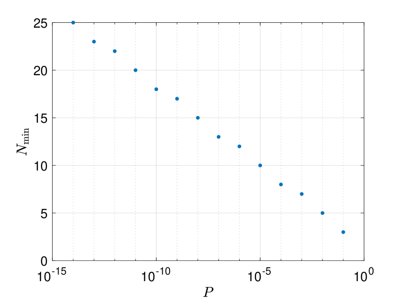
Figure 1: Minimum stabilizing horizon length.

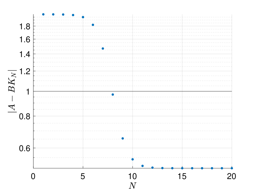
Figure 2: Closed-loop matrix eigenvalues with $P^{\mathrm{f}}=10^{-4}$.

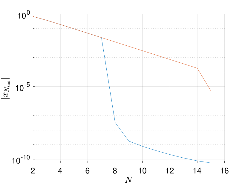
Figure 3: State at time $k=500$ obtained with $P^{\mathrm{f}}=0$ (red) and $P^{\mathrm{f}}=1e-4$ (blue).

VII Conclusions

We have discussed the role of suitably chosen terminal costs in yielding exponential stability in the linear-quadratic case by establishing a strong connection to the symmetric solutions of the associated (reverse) discrete-time algebraic Riccati equation. We have connected our results to those obtained for the full nonlinear case and we have provided simple examples to illustrate our results.

References and Notes

- [1] J. B. Rawlings, D. Q. Mayne, and M. Diehl, Model Predictive Control: Theory, Computation, and Design, 2nd ed. Nob Hill Publishing, 2017.
- [2] L. Grüne and J. Pannek, Nonlinear Model Predictive Control, 2nd ed., ser. Communications and Control Engineering. Springer International Publishing, 2017.
- [3] M. Diehl, R. Amrit, and J. B. Rawlings, “A Lyapunov function for economic optimizing model predictive control,” IEEE Trans. Autom. Control, vol. 56, pp. 703–707, 2011.
- [4] R. Amrit, J. Rawlings, and D. Angeli, “Economic optimization using model predictive control with a terminal cost,” Annual Reviews in Control, vol. 35, pp. 178–186, 2011.
- [5] M. Zanon and T. Faulwasser, “Economic MPC without terminal constraints: Gradient-correcting end penalties enforce asymptotic stability,” Journal of Process Control, vol. 63, pp. 1 – 14, 2018.
- [6] J. Willems, “Dissipative Dynamical Systems Part I: General Theory,” Archive for Rational Mechanics and Analysis, vol. 45, no. 5, pp. 321–351, 1972.
- [7] ——, “Dissipative Dynamical Systems Part II: Linear Systems with Quadratic Supply Rates,” Archive for Rational Mechanics and Analysis, vol. 45, no. 5, pp. 352–393, 1972.
- [8] J. C. Willems, “Least Squares Stationary Optimal Control and the Algebraic Riccati Equation,” IEEE Transactions on Automatic Control, vol. AC-16, no. 6, pp. 621–634, 1971.
- [9] T. Damm, L. Grüne, M. Stieler, and K. Worthmann, “An exponential turnpike theorem for dissipative discrete time optimal control problems,” SIAM J. Control Optim., vol. 52, no. 3, pp. 1935–1957, 2014.
- [10] L. Grüne and R. Guglielmi, “Turnpike properties and strict dissipativity for discrete time linear quadratic optimal control problems,” SIAM Journal on Control and Optimization, vol. 56, no. 2, pp. 1282–1302, 2018.
- [11] L. Grüne and M. Zanon, “Stabilization of strictly pre-dissipative nonlinear receding horizon control by terminal costs,” 2024. [Online]. Available: https://arxiv.org/abs/2412.13538
- [12] M. Diehl, R. Amrit, and J. Rawlings, “A Lyapunov Function for Economic Optimizing Model Predictive Control,” IEEE Trans. of Automatic Control, vol. 56, no. 3, pp. 703–707, March 2011.
- [13] D. Angeli, R. Amrit, and J. Rawlings, “On Average Performance and Stability of Economic Model Predictive Control,” IEEE Transactions on Automatic Control, vol. 57, pp. 1615 – 1626, 2012.
- [14] T. Faulwasser, L. Grüne, and M. Müller, “Economic nonlinear model predictive control: Stability, optimality and performance,” Foundations and Trends in Systems and Control, vol. 5, no. 1, pp. 1–98, 2018.
- [15] M. A. Müller, D. Angeli, and F. Allgöwer, “On necessity and robustness of dissipativity in economic model predictive control,” IEEE Transactions on Automatic Control, vol. 60, no. 6, pp. 1671–1676, 2015.
- [16] M. Müller, D. Angeli, and F. Allgöwer, “On convergence of averagely constrained economic MPC and necessity of dissipativity for optimal steady-state operation,” in Proceedings of the American Control Conference, 2013.
- [17] T. Faulwasser and M. Zanon, “Asymptotic Stability of Economic NMPC: The Importance of Adjoints,” in Proceedings of the IFAC Nonlinear Model Predictive Control Conference, 2018.
- [18] L. Grüne, “Economic receding horizon control without terminal constraints,” Automatica, vol. 49, pp. 725–734, 2013.
- [19] M. A. Müller and L. Grüne, “Economic model predictive control without terminal constraints for optimal periodic behavior,” Automatica, vol. 70, pp. 128 – 139, 2016.
- [20] B. P. Molinari, “The Stabilizing Solution of the Discrete Algebraic Riccati Equation,” IEEE Transactions on Automatic Control, vol. 20, pp. 396–399, 1975.
- [21] P. Lancaster, A. C. M. Ran, and L. Rodman, “Hermitian solutions of the discrete algebraic Riccati equation,” International Journal of Control, vol. 44, pp. 777–802, 1986.
- [22] A. C. M. Ran and H. L. Trentelman, “Linear Quadratic Problems with Indefinite Cost for Discrete Time Systems,” SIAM Journal on Matrix Analysis and Applications, vol. 14, pp. 776–797, 1993.
- [23] L. Grüne and M. Stieler, “A Lyapunov function for economic MPC without terminal conditions,” in Proc. of the 53rd IEEE Conference on Decision and Control, December 2014, pp. 2740–2745.
- [24] M. Zanon, S. Gros, and M. Diehl, “Indefinite Linear MPC and Approximated Economic MPC for Nonlinear Systems,” Journal of Process Control, vol. 24, pp. 1273–1281, 2014.
- [25] A. A. Stoorvogel and A. Saberi, “The Discrete Algebraic Riccati Equation and Linear Matrix Inequality,” Linear Algebra and its Applications, vol. 274, no. 1, pp. 317–365, 1998.
- [26] V. Ionescu, “Reverse discrete-time riccati equation and extended nehari’s problem,” Linear Algebra and its Applications, vol. 236, pp. 59–94, 1996.
- [27] M. Zanon, S. Gros, and M. Diehl, “A Tracking MPC Formulation that is Locally Equivalent to Economic MPC,” Journal of Process Control, vol. 45, pp. 30 – 42, 2016.
- [28] B. D. O. Anderson and J. B. Moore, Optimal Control - Linear Quadratic Methods. Dover, 1990.