Complexity and Isotropization based Extended Models in the context of Electromagnetic Field: An Implication of Minimal Gravitational Decoupling

Abstract

This paper formulates three different analytical solutions to the gravitational field equations in the framework of Rastall theory by taking into account the gravitational decoupling approach. For this, the anisotropic spherical interior fluid distribution is assumed as a seed source characterized by the corresponding Lagrangian. The field equations are then modified by introducing an additional source which is gravitationally coupled with the former fluid setup. Since this approach makes the Rastall equations more complex, the MGD scheme is used to tackle this, dividing these equations into two systems. Some particular ansatz are taken into account to solve the first system, describing initial anisotropic fluid. These metric potentials contain multiple constants which are determined with the help of boundary conditions. On the other hand, the solution for the second set is calculated through different well-known constraints. Afterwards, the estimated data of a pulsar $4U1820-30$ is considered so that the feasibility of the developed models can be checked graphically. It is concluded that all resulting models show physically acceptable behavior under certain choices of Rastall and decoupling parameters.

Keywords: Rastall theory; Gravitational decoupling; Complexity; Electric charge; Stability.
PACS: 04.50.Kd; 04.40.-b; 04.40.Dg.

1 Introduction

In 1972, Peter Rastall proposed the notion that the energy-momentum tensor (EMT) having null divergence in flat spacetime may not necessarily vanish in curved spacetime configurations [1]. Since this is the fundamental assumption on which the proposed modification of general theory of relativity (GR) is based, it named the Rastall gravity theory. In this theory, distinct from the Einstein’s GR, the inclusion of the Ricci scalar $R$ is achieved through the introduction of the Rastall parameter. This alteration fundamentally reshapes the interaction between matter fields and gravitational forces, leading to a paradigm shift in the understanding of these phenomena. Within this theoretical framework, emphasis is placed on non-minimal couplings as the primary mechanism governing the dynamics of gravity and matter interactions. When exploring this gravity theory, scientists determined that it stands on par with other modifications of GR obtained by adjusting the Einstein-Hilbert action [2]-[14].

As per the observational status of this theory is concerned, Batista et al. [15] explored the Rastall gravity within the context of FLRW metric and studied the evolution of small perturbations. They concluded that the two developed models dramatically stable under certain parametric values. Fabris et al. [16] have explored the implications of this gravity within a cosmological framework, utilizing data from Type Ia supernovae to investigate the viability of the model. Their findings indicated that while this extended theory can accommodate certain cosmological observations, it does not strictly constrain the parameters involved, preferring values that align closely with those predicted by GR. Darabi and his colleagues [17] argued that the Rastall theory has a non-minimal coupling that could produce interesting results. An intriguing aspect of this theory is its ability to uphold any solution derived from the Einstein’s equations. Notably, when examining black hole configurations, it is explored that both GR and Rastall gravity yield identical outcomes in scenarios involving vacuum spacetime. Some interesting works can be found in [18]-[23].

The celestial structures are typically defined by a set of up to forth order partial differential equations incorporating geometric and matter terms, known as the gravitational field equations. The solutions (extracted either analytically or numerically) of these complex equations have garnered significant attention among astrophysicists in recent times. These solutions enable the evaluation of whether the stellar object being studied possesses physical relevance or not. To address the needs of astronomers, diverse methods have been developed and applied to generate solutions that might be of interest to them [24]-[30]. A notable strategy has been proposed by a research team led by Jorge Ovalle, known as gravitational decoupling. This approach is particularly prominent because it can be employed even when multiple physical factors are involved in the interior geometry. A detailed outline of this method shall be discussed later in the section where it is more relevant. The techniques used to analyze this problem can be broadly categorized into two main approaches. The first method, known as the minimal geometric deformation (MGD), has been pioneered by Ovalle [31] which was extended in [32], who successfully applied it to obtain exact solutions. This approach was subsequently employed by Casadio et al. [33], which led to the development of the Schwarzschild spacetime.

Ovalle et al. [34] incorporated a new fluid source into the initially considered matter composition through a Lagrangian density. This modification led to the generation of novel and promising findings. The study was subsequently extended to include the effects of the Maxwell field. In this case, two Lagrangian densities were considered: one corresponding to the initial source and another representing the electromagnetic field. Subsequently, a third Lagrangian density analogous to the additional source was introduced, further expanding the scope of the investigation and its potential implications [35]. In an effort to explore this strategy, alternative theories were investigated, yielding multiple viable outcomes [36]-[38]. Gabbanelli et al. [39] pursued a similar approach by using Durgapal-Fuloria metric as an original perfect fluid source and developed a physically existing extension. Following the same, researchers have expanded the domain of Tolman VII and Heintzmann isotropic models [40, 41]. Sharif and Naseer [42, 43] have significantly broadened the scope of Ovalle’s work by incorporating both charged and uncharged scenarios in Einstein’s as well as modified frameworks, and reported stable outcomes. Some other interesting works in this regard are [44]-[51].

The scientific community has also devoted significant attention to investigating the factors that contribute to the intricate nature of celestial objects. Numerous definitions have been put forth over time to encapsulate this concept, yet they have been deemed insufficient in certain scenarios. In this regard, Herrera [52], a prominent astrophysicist, recently pioneered the widely accepted definition of complexity. Following his initial work, Herrera and his research team later expanded the definition to encompass situations where heat dissipation plays a crucial role as a dominant factor in the interior spacetime [53]. The underlying motivation for this definition is rooted in orthogonally decomposing the curvature tensor, yielded multiple scalars that are interconnected with various physical parameters. Notably, the primary contributors to the complexity of the system (i.e., density inhomogeneity and pressure anisotropy) are encapsulated within a single scalar, which is thus designated as the complexity factor. Some other factors are also appeared while decomposing the forth rank Riemann tensor, however, they possess incomplete information to be called the complexity factor for the considered fluid configuration.

Recent studies have explored the definition of complexity within the framework of modified theories [54]-[57]. All of their results indicated that the factor $Y_{TF}$ remains the complexity factor, no matters what kind of interior geometry is being studied, either, static/non-static, uncharged/charged, etc. A notable aspect of this study is the reliance on specific conditions to solve the field equations. One such constraint, the vanishing complexity, has garnered significant attention from researchers in recent years. This constraint has been effectively employed in the context of gravitational decoupling to investigate compact models [58]-[60]. Casadio with his colleagues [61] proposed a couple of theoretical constraints, with one model formulated under disappearing complexity condition and the other focusing on the isotropization mechanism. Maurya et al. [62] subsequently delved into these models through the Karmarkar condition, investigating the influence of various parameters on internal complexity and anisotropy in principal pressure. Extending their analysis to incorporate the impact of Brans-Dicke theory, they derived physically meaningful solutions [63].

The solutions to the gravitational equations play a pivotal role in the study of compact objects in GR as well as modified theories of gravity. These solutions provide a framework for modeling the structure and stability of anisotropic neutron stars, which are believed to exhibit complex internal dynamics due to factors such as superfluidity and strong magnetic fields. Recent literature has highlighted the relevance of the Krori-Barua metric in various gravitational contexts, demonstrating its applicability in constructing stable celestial configurations [64]-[67]. Additionally, the Tolman IV solution has been utilized to analyze anisotropic relativistic spheres in modified gravity theories, revealing that these models can satisfy essential physical requirements and avoid singularities [68]-[71]. By leveraging these solutions, researchers can better understand the intricate balance between gravitational forces and internal pressures in compact stars, providing valuable constraints on their mass and radius based on observational data. Consequently, the utilization of both these spacetimes into astrophysical models not only enhances our understanding of stellar structures but also contributes to the ongoing discourse on the viability of Rastall theory, thereby paving the way for future research in the field.

This article explores the effects of specific parameters on the newly derived charged models within the framework of Rastall gravity. To address the corresponding field equations, various constraints are applied, drawing from the idea of isotropization and complexity. The structure of this paper is outlined below. The origin of Rastall theory and the inclusion of an additional source term are explained in the following section. Section 3 outlines the MGD approach in detail and also explains its implementation. In sections 4 and 5, I derive three innovative solutions using analytical methods. These solutions are also visualized and discussed through graphical representations. Finally, section 6 provides a summary of the results obtained within the present scenario. As a statement of research hypothesis, the Rastall theory, when applied to spherically symmetric spacetime with anisotropic pressures, yields physically viable models that can describe the structure and behavior of neutron stars, providing insights that extend beyond those offered by GR.

2 Fundamentals of Rastall Theory and Static Spherical Spacetime

General relativity is based on the fundamental concept of the conservation of EMT within the spacetime geometry under discussion. When this result does not hold within a curved spacetime scenario, i.e., the EMT becomes non-conserved, Rastall theory come into being [1]. The gravitational equations under respective modification become

$$G_{\eta\mu}\equiv R_{\eta\mu}-\frac{1}{2}Rg_{\eta\mu}=\kappa\big{(}T_{\eta\mu}-\xi Rg_{\eta\mu}\big{)},$$ (1)

where

• $R_{\eta\mu}$ and $G_{\eta\mu}$ denote the Ricci tensor and Einstein tensor, respectively,

• $T_{\eta\mu}$ symbolizes the fluid distribution and $\kappa$ being the coupling constant,

• $\xi$ refers to the Rastall parameter under the control of which this theory differs from the standard GR.

It is exciting to know that there is a consistency between the field equations (1) and the following non-conservation phenomenon defined as

$$\nabla^{\eta}T_{\eta\mu}=\xi g_{\eta\mu}\nabla^{\eta}R,$$ (2)

which obviously results in the conservation equation for $\xi=0$. It must also be stated that the so-called non-minimal interaction between matter and spacetime can be observed on the evolution of celestial objects under the above non-zero divergence. If we define the factor

$$\hat{T}_{\eta\mu}=T_{\eta\mu}-\xi Rg_{\eta\mu},$$ (3)

this helps in redefining the equations of motion (1) in the following

$$G_{\eta\mu}=\kappa\hat{T}_{\eta\mu},$$ (4)

and, hence, they are compatible with the mathematical result expressed by $\nabla^{\eta}\hat{T}_{\eta\mu}=0$. We also observe that the same result can be obtained for extended theories which are achieved through the modification of the action function.

To reframe the field equations (1), we begin by taking their trace. This yields

$$R=\frac{\kappa T}{4\xi\kappa-1},$$ (5)

which after substituting this into Eq.(3) gives the effective matter part as

$$\bar{T}_{\eta\mu}=T_{\eta\mu}-\frac{\beta T}{4\beta-1}g_{\eta\mu},$$ (6)

where $\beta=\xi\kappa$. For the current analysis, we set $\kappa=1$, which implies $\beta=\xi$. It is crucial to note that the one can obtain compact structures which are physically realistic only for the values of $\beta$ other than $\frac{1}{4}$.

The presence of anisotropy in the interiors of compact stars is a fundamental topic in astrophysics, profoundly affecting their structural and dynamic characteristics. Anisotropy denotes the variation in pressure within a star, specifically where radial pressure does not equal the tangential one. This phenomenon becomes especially significant in high-density environments, such as neutron stars, where extreme gravitational and magnetic forces can cause notable departures from isotropic profile. Research on anisotropic models has progressed since the early 20^th century, with key studies emphasizing the importance of incorporating anisotropic pressure into stellar modeling. Various investigations have established that anisotropic pressures can emerge due to several factors (such as rotation, magnetic fields, and phase transitions in stellar matter [72]-[76]). This can be written as [77]

$$T_{\eta\mu}=(\rho+P_{t})v_{\eta}v_{\mu}+P_{t}g_{\eta\mu}-\Pi u_{\eta}u_{\mu},$$ (7)

in which $\Pi=P_{t}-P_{r}$ is the anisotropy (the difference of tangential and radial pressure), $\rho$ is the fluid’s density, $v_{\eta}$ being the four-velocity. Also, the four-vector is defined by $u_{\eta}$.

Our aim is to explore the charge effect on existing stellar structures obtained through the gravitational decoupling. This can only be done if we redefine the matter part of the field equations by adding the electromagnetic tensor $E_{\eta\mu}$ (already defined in the literature) and additional fluid source $\Theta_{\eta\mu}$. Also, keep in mind that the later fluid distribution is added along with a constant, named the decoupling parameter $\zeta$ that controls its influence on the geometry under discussion. The field equations now become as

$$G_{\eta\mu}=\tilde{T}_{\eta\mu},$$ (8)

where

$$\tilde{T}_{\eta\mu}=\bar{T}_{\eta\mu}+E_{\eta\mu}+\zeta\Theta_{\eta\mu},$$ (9)

and the divergence of the above fluid setup yields $\nabla^{\eta}\tilde{T}_{\eta\mu}=0$. The second term guarantees the presence of charge in a geometrical structure and defined as [78]

$$E_{\eta\mu}=\frac{1}{4\pi}\left[\frac{1}{4}g_{\eta\mu}\mathcal{N}^{\tau\nu}\mathcal{N}_{\tau\nu}-\mathcal{N}^{\nu}_{\eta}\mathcal{N}_{\nu\eta}\right],$$

where $\mathcal{N}_{\eta\mu}=\phi_{\mu;\eta}-\phi_{\eta;\mu}$ and $\phi_{\eta}=\phi(r)\delta^{0}_{\eta}$ are the Maxwell field tensor and four-potential, respectively.

A spherical geometry either static or non-static has a great importance in the literature as several researchers believe that the spacetime structures, such as stars, galaxies, etc. are exactly or approximately spherically symmetric. Following this, the interior spherical geometry is defined as

$$ds_{-}^{2}=-e^{\sigma}dt^{2}+e^{\alpha}dr^{2}+r^{2}\big{(}d\theta^{2}+\sin^{2}\theta d\phi^{2}\big{)},$$ (10)

with $\alpha=\alpha(r)$ and $\sigma=\sigma(r)$, showing that the above metric do not admit change over time. This metric helps in defining some already expressed tensor quantities in the following way

$$v^{\eta}=\delta^{\eta}_{0}e^{\frac{-\sigma}{2}},\quad u^{\eta}=\delta^{\eta}_{1}e^{\frac{-\alpha}{2}}.$$ (11)

They are found to agree with certain relations such as $u^{\eta}v_{\eta}=0,~u^{\eta}u_{\eta}=1$ and $v^{\eta}v_{\eta}=-1$.

By taking Eqs.(8), (9) and (10) into account simultaneously, we get the gravitational equations as

$$e^{-\alpha}\left(\frac{\alpha^{\prime}}{r}-\frac{1}{r^{2}}\right)+\frac{1}{r^{2}}=\rho-\zeta\Theta_{0}^{0}+\frac{q^{2}}{r^{4}}+\frac{\beta}{4\beta-1}\left(P_{r}+2P_{t}-\rho\right),$$ (12)

$$e^{-\alpha}\left(\frac{1}{r^{2}}+\frac{\sigma^{\prime}}{r}\right)-\frac{1}{r^{2}}=P_{r}+\zeta\Theta_{1}^{1}-\frac{q^{2}}{r^{4}}-\frac{\beta}{4\beta-1}\left(P_{r}+2P_{t}-\rho\right),$$ (13)

$$\frac{e^{-\alpha}}{4}\left[\sigma^{\prime 2}-\alpha^{\prime}\sigma^{\prime}+2\sigma^{\prime\prime}-\frac{2\alpha^{\prime}}{r}+\frac{2\sigma^{\prime}}{r}\right]=P_{t}+\zeta\Theta_{2}^{2}+\frac{q^{2}}{r^{4}}-\frac{\beta}{4\beta-1}\left(P_{r}+2P_{t}-\rho\right),$$ (14)

where in the above expressions, prime means $\frac{\partial}{\partial r}$. Also, the terms accompanied by the factor involving $\beta$ represent the Rastall effect. By employing the metric specified in Eq.(10), we can expand the conservation equation, which must involve additional terms depending on the considered specific context as

$$\frac{dP_{r}}{dr}+\frac{\sigma^{\prime}}{2}\left(\rho+P_{r}\right)+\frac{\zeta\sigma^{\prime}}{2}\left(\Theta_{1}^{1}-\Theta_{0}^{0}\right)+\frac{2}{r}\left(P_{r}-P_{t}\right)$$

$$+\zeta\frac{d\Theta_{1}^{1}}{dr}+\frac{2\zeta}{r}\left(\Theta_{1}^{1}-\Theta_{2}^{2}\right)-\frac{qq^{\prime}}{r^{4}}=\frac{\beta}{1-4\beta}\big{(}\rho^{\prime}-P_{r}^{\prime}-2P_{t}^{\prime}\big{)}.$$ (15)

The significance of Eq.(15) lies in its utility for investigating evolutionary transformations within self-gravitating systems. It is noteworthy that the incorporation of an additional source term and charge in the initial anisotropic setup introduces more complications, allowing for a more comprehensive description of the system’s dynamics. Equivalently, we can say that the number of unknowns are increased, specifically to $(\sigma$,$\alpha$,$\rho$,$P_{r}$,$P_{t}$,$q$,$\Theta_{0}^{0}$,$\Theta_{1}^{1}$,$\Theta_{2}^{2})$. As a result, additional constraints must be applied to ensure the solvability.

3 Application of Minimal Geometric Deformation

Recall that the extra source is gravitationally coupled to the initial analogue, and could be the scalar/vector/tensor field. It must be stressed here that finding the solution to the gravitational equations containing multiple physical factors is highly difficult due to their non-linear nature. This complication can be reduced if we utilize a well-known and systematic technique which has been suggested by Herrera [34] in recent years so that the under-determined system (12)-(14) can be handled. This is referred to the gravitational decoupling as the equations are decoupled into different sets in this technique. The idea behind this strategy is that a new metric must be assumed so that the previously determined field equations can be transformed into a new reference frame in which the resulting systems of equations are easy to solve. We now execute this by introducing a new metric of the form

$$ds_{-}^{2}=-e^{\gamma(r)}dt^{2}+\frac{1}{\chi(r)}dr^{2}+r^{2}\big{(}d\theta^{2}+\sin^{2}\theta d\phi^{2}\big{)}.$$ (16)

The radial and temporal metric components are of great importance in this scheme because the transformations are implemented on them. These transformations are

$$\gamma\rightarrow\sigma=\gamma+\zeta t,\quad\chi\rightarrow e^{-\alpha}=\chi+\zeta f,$$ (17)

where

• $t$ is the temporal deformation function,

• $f$ is that corresponding to the radial component.

This article centers on the application of MGD method, which ensures that the temporal metric potential remains unchanged. By expressing the two functions as $t\rightarrow 0,~f\rightarrow d_{f}$, we can then combine this with Eq.(17) to get

$$\gamma\rightarrow\sigma=\gamma,\quad\chi\rightarrow e^{-\alpha}=\chi+\zeta d_{f},$$ (18)

where $d_{f}=d_{f}(r)$. The fascinating aspect of these transformations is that they are helpful for maintaining the spherical object’s symmetry. By applying them to Eqs.(12)-(14), we obtain two distinct systems. The first system arises when $\zeta=0$, which effectively eliminates the influence of the newly introduced matter setup, as indicated by the following expression

$$e^{-\alpha}\left(\frac{\alpha^{\prime}}{r}-\frac{1}{r^{2}}\right)+\frac{1}{r^{2}}=\rho+\frac{q^{2}}{r^{4}}+\frac{\beta}{4\beta-1}\left(P_{r}+2P_{t}-\rho\right),$$ (19)

$$e^{-\alpha}\left(\frac{1}{r^{2}}+\frac{\sigma^{\prime}}{r}\right)-\frac{1}{r^{2}}=P_{r}-\frac{q^{2}}{r^{4}}-\frac{\beta}{4\beta-1}\left(P_{r}+2P_{t}-\rho\right),$$ (20)

$$\frac{e^{-\alpha}}{4}\left[\sigma^{\prime 2}-\alpha^{\prime}\sigma^{\prime}+2\sigma^{\prime\prime}-\frac{2\alpha^{\prime}}{r}+\frac{2\sigma^{\prime}}{r}\right]=P_{t}+\frac{q^{2}}{r^{4}}-\frac{\beta}{4\beta-1}\left(P_{r}+2P_{t}-\rho\right),$$ (21)

leads to explicit expressions for fluid triplet

$$\rho =\frac{e^{-\alpha}}{2r^{4}}\bigg{[}r^{2}\big{\{}2\big{(}\beta r^{2}\sigma^{\prime\prime}+(r-2\beta r)\alpha^{\prime}+(2\beta-1)\big{(}1-e^{\alpha}\big{)}\big{)}$$

$$+\beta r^{2}\sigma^{\prime 2}+\beta r\sigma^{\prime}\big{(}4-r\alpha^{\prime}\big{)}\big{\}}-2q^{2}e^{\alpha}\bigg{]},$$ (22)

$$P_{r} =\frac{e^{-\alpha}}{2r^{4}}\bigg{[}2q^{2}e^{\alpha}-r^{2}\big{\{}2\big{(}\beta r^{2}\sigma^{\prime\prime}-2\beta r\alpha^{\prime}+(2\beta-1)\big{(}1-e^{\alpha}\big{)}\big{)}$$

$$+\beta r^{2}\sigma^{\prime 2}-r\sigma^{\prime}\big{(}-4\beta+\beta r\alpha^{\prime}+2\big{)}\big{\}}\bigg{]},$$ (23)

$$P_{t} =\frac{-e^{-\alpha}}{4r^{4}}\bigg{[}r^{2}\big{\{}8\beta+4\beta r^{2}\sigma^{\prime\prime}+(2\beta-1)r^{2}\sigma^{\prime 2}-2r^{2}\sigma^{\prime\prime}+r\sigma^{\prime}$$

$$\times\big{(}8\beta+(r-2\beta r)\alpha^{\prime}-2\big{)}+(2-8\beta)r\alpha^{\prime}-8\beta e^{\alpha}\big{\}}+4q^{2}e^{\alpha}\bigg{]}.$$ (24)

On the other hand, the system which includes the effect of a new source only is achieved as

$$\Theta_{0}^{0}=\frac{{d_{f}}^{\prime}}{r}+\frac{d_{f}}{r^{2}},$$ (25)

$$\Theta_{1}^{1}=d_{f}\left(\frac{\sigma^{\prime}}{r}+\frac{1}{r^{2}}\right),$$ (26)

$$\Theta_{2}^{2}=\frac{d_{f}}{4}\left(2\sigma^{\prime\prime}+\sigma^{\prime 2}+\frac{2\sigma^{\prime}}{r}\right)+{d_{f}}^{\prime}\left(\frac{\sigma^{\prime}}{4}+\frac{1}{2r}\right).$$ (27)

The MGD approach is notable for its ability to decouple fluid sources, thereby preventing energy exchange between them. This decoupling allows the sources to be conserved individually. We can now proceed to find the solutions for each of the resulting systems one by one. We observe six unknowns ($\rho$,$P_{r}$,$P_{t}$,$\sigma$,$\alpha$,$q$) in Eqs.(22)-(24), leading us to adopt an ansatz from the existing literature. Additionally, four unknowns ($d_{f}$, $\Theta_{0}^{0}$, $\Theta_{1}^{1}$, $\Theta_{2}^{2}$) are present in Eqs.(25)-(27). To proceed, we shall impose constraints on the $\Theta$-sector in the following sections. At this point, it is crucial to specify the effective fluid triplet as

$$\tilde{\rho}=\rho-\zeta\Theta_{0}^{0},\quad\tilde{P}_{r}=P_{r}+\zeta\Theta_{1}^{1},\quad\tilde{P}_{t}=P_{t}+\zeta\Theta_{2}^{2}.$$ (28)

The following anisotropy aligns with the total fluid configuration, and we express it as

$$\tilde{\Pi}=\tilde{P}_{t}-\tilde{P}_{r}=\Pi+\Pi_{\Theta},$$ (29)

where $\Pi_{\Theta}=\zeta(\Theta_{2}^{2}-\Theta_{1}^{1})$ corresponds to the new source.

4 Shift from Anisotropic Matter Distribution to Isotropic Analogue

Assuming that the anisotropy $\tilde{\Pi}$ given by Eq.(29) corresponds to the both matter distributions within the interior fluid, we shall now investigate the consequences on the massive structure if this factor deviates from the one corresponding solely to the initially assumed source. In light of the preceding discussion, we introduce a constraint that assumes the seed source becomes isotropic when another source is added, governed by the parameter $\zeta$. It is essential to note that this assumption is a mathematical construct that is valid only for a specific value of this parameter. The constraint is given below as

$$\Pi_{\Theta}=-\Pi\quad\Rightarrow\quad\Theta_{1}^{1}-\Theta_{2}^{2}=P_{t}-P_{r}.$$ (30)

Recently, Casadio et al. [61] utilized this approach in their analysis on decoupled models, where they transformed the anisotropic sphere into its isotropic counterpart. Since we need to tackle both sets of equations individually, we adopt $q(r)=\omega r^{3}$ with $\omega$ has a dimension of $\frac{1}{\ell^{2}}$ [79] along with the Krori-Barua spacetime to handle the first system as [80]

$$\sigma(r) =a_{1}r^{2}+a_{2},$$ (31)

$$\chi(r) =e^{-\alpha}=e^{-a_{3}r^{2}},$$ (32)

$$\rho =\frac{e^{-a_{3}r^{2}}}{r^{2}}\big{[}2\beta a_{1}^{2}r^{4}+2(1-2\beta)a_{3}r^{2}-2\beta a_{1}r^{2}\big{(}a_{3}r^{2}-3\big{)}$$

$$-2\beta e^{a_{3}r^{2}}+e^{a_{3}r^{2}}-r^{4}\omega^{2}e^{a_{3}r^{2}}+2\beta-1\big{]},$$ (33)

$$P_{r} =\frac{e^{-a_{3}r^{2}}}{r^{2}}\big{[}4\beta a_{3}r^{2}-2\beta a_{1}^{2}r^{4}+2a_{1}r^{2}\big{(}\beta a_{3}r^{2}-3\beta+1\big{)}+1$$

$$+2\beta e^{a_{3}r^{2}}-e^{a_{3}r^{2}}+r^{4}\omega^{2}e^{a_{3}r^{2}}-2\beta\big{]},$$ (34)

$$P_{t} =\frac{e^{-a_{3}r^{2}}}{r^{2}}\big{[}(1-2\beta)a_{1}^{2}r^{4}+(4\beta-1)a_{3}r^{2}-r^{4}\omega^{2}e^{a_{3}r^{2}}-2\beta$$

$$+2\beta e^{a_{3}r^{2}}+a_{1}r^{2}\big{\{}(2\beta-1)a_{3}r^{2}-6\beta+2\big{\}}\big{]},$$ (35)

containing a set of three constants $(a_{1},a_{2},a_{3})$ which are unknowns at this point. It is necessary to make them known as they shall be used in the graphical analysis of our developed models in subsequent sections. The importance of the above ansatz can be assessed from the aspect that a large body of literature considers this metric to explore physically relevant interior distributions both in GR and its modifications [81, 82].

We now require to perform some calculations at the spherical interface to make the above three constants known. This analysis on the hypersurface refers to the Darmois junction conditions in which both interior and vacuum exterior spacetimes meet at a specific point, named the boundary. The Darmois junction conditions can be categorized into two fundamental forms: the first involves the continuity of the intrinsic geometry across the junction, ensuring that the metric tensor is continuous [83]. The second form addresses the continuity of the extrinsic curvature, which relates to how the two regions bend into each other. This also ensures that the radial pressure falls to zero at finite value of $r$, which is known as the star’s radius. The exterior metric should match with the one considered as the interior region in terms of the properties such as charge, static in nature, etc. We eventually adopt the Reissner-Nordström line element under its mass $\tilde{M}$ and charge $\mathrm{Q}$ as

$$ds_{+}^{2}=-\left(1-\frac{2\tilde{M}}{r}+\frac{\mathrm{Q}^{2}}{r^{2}}\right)dt^{2}+\left(1-\frac{2\tilde{M}}{r}+\frac{\mathrm{Q}^{2}}{r^{2}}\right)^{-1}dr^{2}+r^{2}\big{(}d\theta^{2}+\sin^{2}\theta d\phi^{2}\big{)}.$$ (36)

Using the condition of continuity of metric components of geometries (10) and (36) across the spherical interface provides the following constraints

$$g_{tt}^{-}~{{}_{=}^{\Sigma}}~g_{tt}^{+},\quad g_{rr}^{-}~{{}_{=}^{\Sigma}}~g_{rr}^{+},\quad g_{tt,r}^{-}~{{}_{=}^{\Sigma}}~g_{tt,r}^{+}.$$

Substituting the values in above expressions, we get three equations given by

$$e^{a_{1}\mathrm{R}^{2}+a_{2}} =1-\frac{2\tilde{M}}{\mathrm{R}}+\frac{\mathrm{Q}^{2}}{\mathrm{R}^{2}},$$ (37)

$$e^{a_{3}\mathrm{R}^{2}} =\left(1-\frac{2\tilde{M}}{\mathrm{R}}+\frac{\mathrm{Q}^{2}}{\mathrm{R}^{2}}\right)^{-1},$$ (38)

$$a_{1}\mathrm{R}e^{a_{1}\mathrm{R}^{2}+a_{2}} =\frac{\tilde{M}}{\mathrm{R}^{2}}-\frac{\mathrm{Q}^{2}}{\mathrm{R}^{3}},$$ (39)

whose simultaneous solution is

$$a_{1} = \frac{\tilde{M}\mathrm{R}-\mathrm{Q}^{2}}{\mathrm{R}^{2}\big{(}\mathrm{R}^{2}-2\tilde{M}\mathrm{R}+\mathrm{Q}^{2}\big{)}},$$ (40)

$$a_{2} = \ln\bigg{(}1-\frac{2\tilde{M}}{\mathrm{R}}+\frac{\mathrm{Q}^{2}}{\mathrm{R}^{2}}\bigg{)}-\frac{\tilde{M}\mathrm{R}-\mathrm{Q}^{2}}{\mathrm{R}^{2}-2\tilde{M}\mathrm{R}+\mathrm{Q}^{2}},$$ (41)

$$a_{3} = -\frac{1}{\mathrm{R}^{2}}\ln\bigg{(}1-\frac{2\tilde{M}}{\mathrm{R}}+\frac{\mathrm{Q}^{2}}{\mathrm{R}^{2}}\bigg{)}.$$ (42)

Here, $a_{1}$ and $a_{3}$ have dimension of $\frac{1}{\ell^{2}}$ whereas $a_{2}$ is dimensionless. As we can from Eqs.(40)-(42), the constants are evaluated in term of experimental data of a compact star model such as its mass and radius. We, therefore, consider $4U1820-30$ along with $\tilde{M}=1.58\pm 0.06M_{\bigodot}$ and $\mathrm{R}=9.1\pm 0.4km$ [84]. Further, the term $\mathrm{Q}$ shall take different values in graphical analysis to check its impact on the interior fluid distribution. Merging gravitational equations with (30)-(32) results in

$$a_{1}r^{3}\big{\{}{d_{f}}^{\prime}(r)-2a_{3}re^{-a_{3}r^{2}}\big{\}}+2\big{(}a_{1}^{2}r^{4}-1\big{)}d_{f}(r)-2a_{3}r^{2}e^{-a_{3}r^{2}}$$

$$-2e^{-a_{3}r^{2}}+2a_{1}^{2}r^{4}e^{-a_{3}r^{2}}+r{d_{f}}^{\prime}(r)-4r^{4}\omega^{2}+2=0,$$ (43)

whose analytical solution after performing integration (and thus a constant $c_{1}$ is appeared) becomes

$$d_{f}(r) =\frac{1}{e^{1+a_{1}r^{2}}a_{1}}\big{[}2\omega^{2}r^{2}\text{Ei}\big{(}a_{1}r^{2}+1\big{)}-a_{1}^{2}r^{2}\text{Ei}\big{(}a_{1}r^{2}+1\big{)}$$

$$+ea_{1}\big{\{}e^{a_{1}r^{2}}-e^{(a_{1}-a_{3})r^{2}}\big{\}}\big{]}+c_{1}r^{2}e^{-a_{1}r^{2}}.$$ (44)

When we merge the above equation with (18), the $g_{rr}$ potential is obtained as

$$e^{\alpha}=\chi^{-1} =\bigg{[}e^{-a_{3}r^{2}}+\frac{\zeta}{e^{1+a_{1}r^{2}}a_{1}}\big{\{}2\omega^{2}r^{2}\text{Ei}\big{(}a_{1}r^{2}+1\big{)}-a_{1}^{2}r^{2}\text{Ei}\big{(}a_{1}r^{2}+1\big{)}$$

$$+ea_{1}\big{(}e^{a_{1}r^{2}}-e^{(a_{1}-a_{3})r^{2}}\big{)}\big{\}}+c_{1}\zeta r^{2}e^{-a_{1}r^{2}}\bigg{]}^{-1}.$$ (45)

Hence, the solution to the Rastall equations of motion, achieved through the MGD approach, is represented by the following spacetime metric

$$ds_{-}^{2} =-e^{a_{1}r^{2}+a_{2}}dt^{2}+\bigg{[}e^{-a_{3}r^{2}}+\frac{\zeta}{e^{1+a_{1}r^{2}}a_{1}}\big{\{}2\omega^{2}r^{2}\text{Ei}\big{(}a_{1}r^{2}+1\big{)}$$

$$-a_{1}^{2}r^{2}\text{Ei}\big{(}a_{1}r^{2}+1\big{)}+ea_{1}\big{(}e^{a_{1}r^{2}}-e^{(a_{1}-a_{3})r^{2}}\big{)}\big{\}}+c_{1}\zeta r^{2}e^{-a_{1}r^{2}}\bigg{]}^{-1}dr^{2}$$

$$+r^{2}\big{(}d\theta^{2}+\sin^{2}\theta d\phi^{2}\big{)}.$$ (46)

This metric describes the interior configuration of the fluid, which is determined by the following fluid variables as

$$\tilde{\rho} =a_{1}\big{\{}2c_{1}\zeta r^{2}e^{-a_{1}r^{2}}+3\zeta e^{-a_{1}r^{2}-1}\text{Ei}\big{(}a_{1}r^{2}+1\big{)}-2\beta a_{3}r^{2}e^{-a_{3}r^{2}}+6\beta e^{-a_{3}r^{2}}\big{\}}$$

$$-3c_{1}\zeta e^{-a_{1}r^{2}}+2a_{1}^{2}r^{2}\bigg{\{}\beta e^{-a_{3}r^{2}}-\zeta e^{-a_{1}r^{2}-1}\text{Ei}\big{(}a_{1}r^{2}+1\big{)}+\frac{\zeta}{a_{1}r^{2}+1}\bigg{\}}+\frac{1}{r^{2}}$$

$$+4\zeta r^{2}\omega^{2}e^{-a_{1}r^{2}-1}\text{Ei}\big{(}a_{1}r^{2}+1\big{)}-\frac{6\zeta\omega^{2}e^{-a_{1}r^{2}-1}\text{Ei}\big{(}a_{1}r^{2}+1\big{)}}{a_{1}}-\frac{4\zeta r^{2}\omega^{2}}{a_{1}r^{2}+1}$$

$$-2a_{3}(2\beta+\zeta-1)e^{-a_{3}r^{2}}+\frac{2\beta e^{-a_{3}r^{2}}}{r^{2}}+\frac{\zeta e^{-a_{3}r^{2}}}{r^{2}}-\frac{e^{-a_{3}r^{2}}}{r^{2}}-\frac{2\beta}{r^{2}}-\frac{\zeta}{r^{2}}-r^{2}\omega^{2},$$ (47)

$$\tilde{P}_{r} =\frac{e^{-a_{3}r^{2}}}{r^{2}}\big{[}4\beta a_{3}r^{2}-2\beta a_{1}^{2}r^{4}+2a_{1}r^{2}\big{(}\beta a_{3}r^{2}-3\beta+1\big{)}+2\beta e^{a_{3}r^{2}}-e^{a_{3}r^{2}}+1$$

$$+r^{4}\omega^{2}e^{a_{3}r^{2}}-2\beta\big{]}+\frac{\zeta e^{-a_{1}r^{2}-1}\big{(}2a_{1}r^{2}+1\big{)}}{a_{1}r^{2}}\big{[}ea_{1}\big{\{}e^{a_{1}r^{2}}-e^{(a_{1}-a_{3})r^{2}}+c_{1}r^{2}\big{\}}$$

$$+2r^{2}\omega^{2}\text{Ei}\big{(}a_{1}r^{2}+1\big{)}-a_{1}^{2}r^{2}\text{Ei}\big{(}a_{1}r^{2}+1\big{)}\big{]},$$ (48)

$$\tilde{P}_{t} =\frac{e^{-a_{1}r^{2}-a_{3}r^{2}-1}}{a_{1}r^{2}}\big{[}a_{1}^{2}r^{2}\big{\{}5c_{1}\zeta r^{2}e^{a_{3}r^{2}+1}-\zeta e^{a_{3}r^{2}}\text{Ei}\big{(}a_{1}r^{2}+1\big{)}+a_{3}(2\beta+\zeta-1)$$

$$\times r^{2}e^{a_{1}r^{2}+1}-6\beta e^{a_{1}r^{2}+1}-5\zeta e^{a_{1}r^{2}+1}+5\zeta e^{a_{1}r^{2}+a_{3}r^{2}+1}+2e^{a_{1}r^{2}+1}\big{\}}+a_{1}\big{(}c_{1}\zeta$$

$$\times r^{2}e^{a_{3}r^{2}+1}+10\zeta r^{4}\omega^{2}e^{a_{3}r^{2}}\text{Ei}\big{(}a_{1}r^{2}+1\big{)}+a_{3}r^{2}(4\beta+\zeta-1)e^{a_{1}r^{2}+1}-2\beta e$$

$$\times e^{a_{1}r^{2}}+2\beta e^{a_{1}r^{2}+a_{3}r^{2}+1}+2\zeta r^{4}\omega^{2}e^{a_{1}r^{2}+a_{3}r^{2}+1}-r^{4}\omega^{2}e^{a_{1}r^{2}+a_{3}r^{2}+1}\big{)}+2\zeta r^{2}\omega^{2}$$

$$\times e^{a_{3}r^{2}}\text{Ei}\big{(}a_{1}r^{2}+1\big{)}-a_{1}^{3}r^{4}\big{\{}5\zeta e^{a_{3}r^{2}}\text{Ei}\big{(}a_{1}r^{2}+1\big{)}+(2\beta+\zeta-1)e^{a_{1}r^{2}+1}\big{\}}\big{]},$$ (49)

and the anisotropic factor becomes in this scenario as

$$\tilde{\Pi}=\frac{e^{-a_{3}r^{2}}}{r^{2}}\big{(}a_{1}^{2}r^{4}-a_{1}a_{3}r^{4}-a_{3}r^{2}+e^{a_{3}r^{2}}-2r^{4}\omega^{2}e^{a_{3}r^{2}}-1\big{)}\big{(}1-\zeta\big{)}.$$ (50)

We clearly see from the above equation that the substitution of $\zeta=1$ results in the vanishing anisotropy. Hence, we can say that the first unique solution (47)-(50) to the charged field equations belong to $\zeta\in[0,1]$. It is also needed to mention that conversion of anisotropic to the isotropic analogue or vice versa depends on the variation of the decoupling parameter within the mentioned range.

4.1 Physical Acceptability Requirements and their Graphical Confirmation

Some properties are necessary to be checked in the interior fluid distribution corresponding to the resulting model so that its physical feasibility can be assessed. We start off from the spherical mass expressed by the following differential equation [85, 86]

$$m^{\prime}(r)=\frac{1}{2}\tilde{\rho}r^{2}\quad\mathrm{or}\quad m(r)=\frac{1}{2}\int_{0}^{r}\tilde{\rho}\tilde{r}^{2}d\tilde{r},$$ (51)

that can be solved either through exact or numerical integration depending on the complexities in the overhead equation. In this case, the effective form of matter’s energy density is provided in Eq.(47). Secondly, a compactness factor must be measured for our geometry which defines the closeness of the particles in any celestial body due to its own gravitational pull. Or in other words, one can express it by the ratio as $\varpi(r)=\frac{m(r)}{r}$ that must be less than $\frac{4}{9}$ in spherical spacetime. This limit has been measured in a study done by Hans Adolph Buchdahl [87] in 1959. Thirdly, another quantity depends on the compactness factor and named the surface redshift. This actually measures the persistent grow (decline) in the wavelength (frequency) of the radiations emitted by heavily compact bodies when they are influenced by other nearby massive objects. This factor is

$$\textrm{z}(r)=\frac{1}{\sqrt{1-2\varpi(r)}}-1,$$ (52)

whose maximum value is classified as

• For isotropic fluid geometry, it is found as 2 [87],

• 5.211 when anisotropy appears in the principal pressure [88].

In evaluating the viability of a model, astrophysicists have put forth certain limitations. Adhering to these constraints ensures the presence of a usual (normal) fluid within the specified interior. Failure to meet these criteria would necessitate the presence of an exotic fluid, thereby impeding the physical viability of stellar structures. These boundaries predominantly rely on the EMT, expresses in the context of anisotropic geometry as

$$\left.\begin{aligned} &\tilde{\rho}+\frac{q^{2}}{r^{4}}\geq 0,\quad\tilde{\rho}+\tilde{P}_{r}\geq 0,\\ &\tilde{\rho}+\tilde{P}_{t}+\frac{2q^{2}}{r^{4}}\geq 0,\quad\tilde{\rho}-\tilde{P}_{r}+\frac{2q^{2}}{r^{4}}\geq 0,\\ &\tilde{\rho}-\tilde{P}_{t}\geq 0,\quad\tilde{\rho}+\tilde{P}_{r}+2\tilde{P}_{t}+\frac{2q^{2}}{r^{4}}\geq 0.\end{aligned}\right\}$$ (53)

Rather than examining all above constraints, one can check only dominant bounds expressed by $\tilde{\rho}-\tilde{P}_{r}+\frac{2q^{2}}{r^{4}}\geq 0$ and $\tilde{\rho}-\tilde{P}_{t}\geq 0$ when all fluid variables lie in the positive range.

Stability is the most important property to be checked when studying stellar models. Here, we shall use two criteria depend on the sound speed discussed below

• It has been proposed in the literature that if the sound speed in both radial ($\tilde{v}_{r}$) and tangential ($\tilde{v}_{t}$) directions are less of the light’s speed, then the model is considered as stable [89]. We can express it as

  $$0<\tilde{v}_{r}=\frac{d\tilde{P}_{r}}{d\tilde{\rho}}<1,\quad 0<\tilde{v}_{t}=\frac{d\tilde{P}_{t}}{d\tilde{\rho}}<1.$$ (54)

• Herrera [90] put forwarded the idea of a cracking in the interior distribution. According to his study, if the inequality

  $$0<|\tilde{v}_{t}-\tilde{v}_{r}|<1,$$ (55)

  satisfies, the system remains stable. Otherwise, it becomes unstable and no more physically relevant.

Now, we explore all the above-mentioned characteristics for our developed model (47)-(50) by varying the parameters involved in these mathematical results. We adopt two, ten and two distinct values of the Rastall parameter $\beta$, decoupling parameter $\zeta$ and charge, respectively. More specifically, we choose $\beta=0.2,0.6$, $\zeta=0.1,0.2,...,1$, $\mathrm{Q}=0.2,0.7$ and $c_{1}=-0.02$. For choosing acceptable value of $c_{1}$, we perform a detailed analysis with its different (small and large) values. By doing so, we come to know that only small but negative value of this constant leads to the meaningful results. Both metric potentials must be positively increasing function of the radial coordinate, however, we only plot the radial component (45) in Figure 1 as the modification is seen only in this component due to the applicability of MGD scheme. The triplet functions such as density and principal pressures (47)-(49) are plotted in Figures 2 and 3 (correspond to lower and upper values of charge), achieving their maximum at $r=0$ and minimum at the interface. It is noticed that the density and both pressures are in direct and inverse relation with $\beta$ and $\mathrm{Q}$. However, increment in $\zeta$ results in decreasing the energy density and increasing pressure ingredients. As the plots of anisotropy are concerned, all of them show nullification of this factor for $\zeta=1$, confirming the presence of mathematical isotropy. However, for all other parametric choices, this function increases with the rise in $r$.

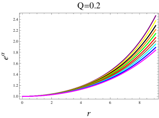
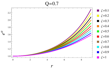
Figure 1: Radial metric (45).

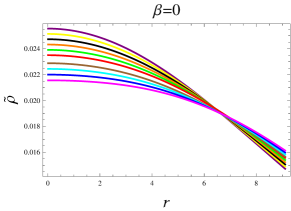
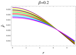
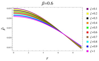
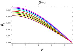
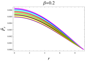
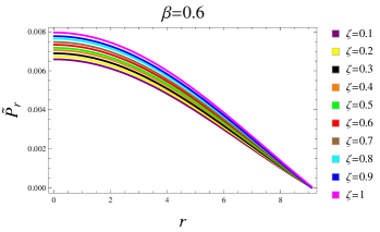
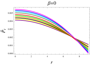
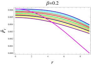
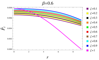
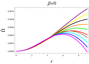
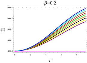
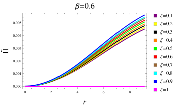
Figure 2: Matter variables corresponding to $\mathrm{Q}=0.2$.

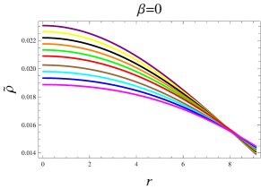
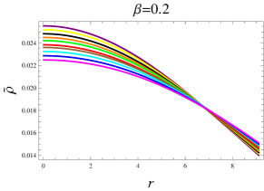
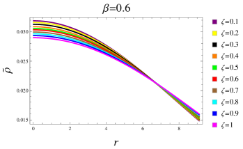
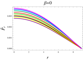
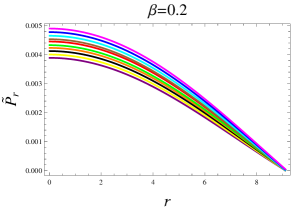
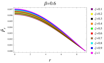
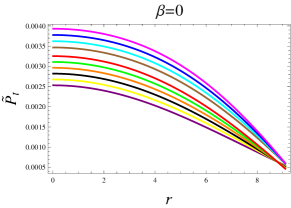
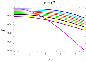
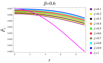
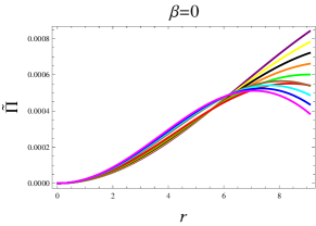
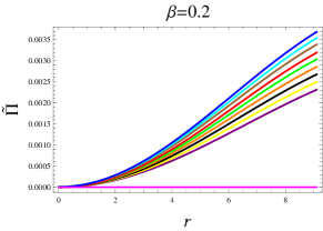
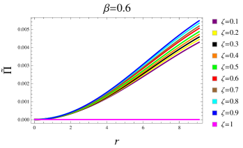
Figure 3: Matter variables corresponding to $\mathrm{Q}=0.7$.

Since the mass function depends on the density of fluid (defined in Eq.(51)), we plot this for all parametric variations and find its increasing profile w.r.t. $r$. We find the more dense interior corresponding to this model for $\beta=0.6$, $\zeta=0.1$ and $\mathrm{Q}=0.2$. The numerical values of the mass function for the previous parametric choices of $\beta$ and $\zeta$ are $\tilde{M}=1.644M_{\bigodot}$ and $1.609M_{\bigodot}$ for $Q=0.2$ and $0.7$, respectively. However, the best fit mass with the observed data is found for lower choices of $\zeta$ and higher values of the electric charge. We also check other two factors (redshift and compactness), however, their graphs are not included here. The energy conditions admitting the difference between density and pressures are checked without adding their graphs. All of them show positive profile of both constraints, hence, we refer this model to be physically viable. The presence of the usual matter is also confirmed. Furthermore, both stability criteria are explored in Figures 4 and 5, respectively. All plots in both these Figures lie in their desired range. This implies that the resulting model corresponding to the constraint (30) is stable.

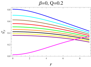
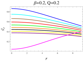
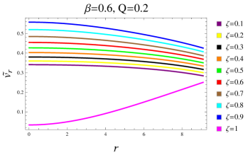
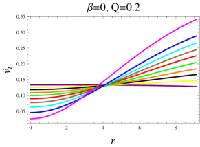
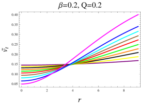
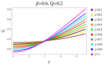
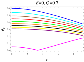
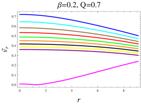
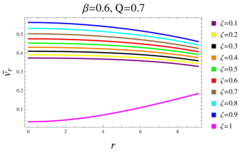
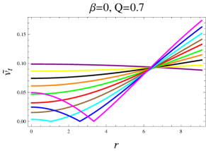
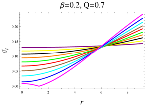
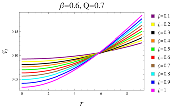
Figure 4: Sound speeds in radial and tangential directions.

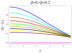
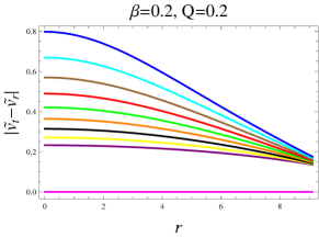
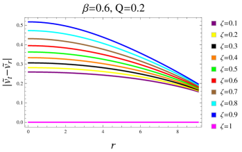
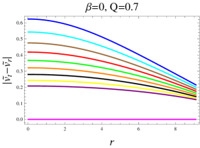
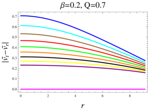
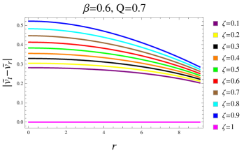
Figure 5: Herrera’s cracking criteria.

5 Complexity Factor and its Implication in Compact Matter Source

The study of astronomical structures has garnered substantial attention from researchers in recent years. Herrera’s work on a static sphere highlights that the physical factors producing complexity play a crucial role in the evolution of compact stars, shedding new light on the intricate dynamics of these celestial bodies [52]. The concept was further developed to account for non-static dynamical fluid setup [53]. By performing an orthogonal splitting of the Riemann-Christoffel tensor, several distinct scalars are identified. It is observed that the two primary factors influencing fluid content (namely density inhomogeneity and anisotropic pressure) are incorporated into one of these scalars, which Herrera referred to as the complexity factor, denoted as $Y_{TF}$ (for more details, see [91]-[97]). This is mathematically represented as

$$Y_{TF}(r)=\Pi+\frac{4q^{2}}{r^{4}}-\frac{1}{2r^{3}}\int_{0}^{r}\tilde{r}^{3}\rho^{\prime}(\tilde{r})d\tilde{r}-\frac{3}{r^{3}}\int_{0}^{r}\frac{qq^{\prime}}{\tilde{r}}d\tilde{r}.$$ (56)

The above equation denotes the complexity factor for the anisotropic fluid distribution influenced by an electromagnetic field. Extending the same definition for our current scenario where two fluid sources are present, Eq.(56) switches into

$$\tilde{Y}_{TF}(r) = \tilde{\Pi}+\frac{4q^{2}}{r^{4}}-\frac{1}{2r^{3}}\int_{0}^{r}\tilde{r}^{3}\tilde{\rho}^{\prime}(\tilde{r})d\tilde{r}-\frac{3}{r^{3}}\int_{0}^{r}\frac{qq^{\prime}}{\tilde{r}}d\tilde{r}$$ (57)

$$= Y_{TF}+Y_{TF}^{\Theta},$$

where

• $Y_{TF}$ corresponds to the geometry defined by Eqs.(22)-(24),

• $Y_{TF}^{\Theta}$ being the complexity factor in relation with the newly added source represented by Eqs.(25)-(27).

Further, they have the values as follows

$$Y_{TF} = \Pi+\frac{4q^{2}}{r^{4}}-\frac{1}{2r^{3}}\int_{0}^{r}\tilde{r}^{3}\rho^{\prime}(\tilde{r})d\tilde{r}-\frac{3}{r^{3}}\int_{0}^{r}\frac{qq^{\prime}}{\tilde{r}}d\tilde{r},$$ (58)

$$Y_{TF}^{\Theta} = \Pi_{\Theta}+\frac{1}{2r^{3}}\int_{0}^{r}\tilde{r}^{3}\Theta{{}_{0}^{0}}^{\prime}(\tilde{r})d\tilde{r}.$$ (59)

Recall that the first resulting solution expressed by Eqs.(47)-(50) corresponded to $\tilde{\Pi}=0$ (isotropization of anisotropic model). In view of this, Eq.(57) becomes

$$\tilde{Y}_{TF} = \frac{4q^{2}}{r^{4}}-\frac{1}{2r^{3}}\int_{0}^{r}\tilde{r}^{3}\tilde{\rho}^{\prime}(\tilde{r})d\tilde{r}-\frac{3}{r^{3}}\int_{0}^{r}\frac{qq^{\prime}}{\tilde{r}}d\tilde{r}.$$ (60)

This along with the fluid’s density (47) turns into

$$\tilde{Y}_{TF} =a_{1}^{2}\bigg{\{}r^{2}\big{(}\zeta\tau_{1}e^{-a_{1}r^{2}-1}-\beta e^{-a_{3}r^{2}}\big{)}-\frac{3\beta e^{-a_{3}r^{2}}}{2a_{3}}-\frac{9\beta e^{-a_{3}r^{2}}}{4a_{3}^{2}r^{2}}+\tau_{2}\bigg{\}}$$

$$+a_{3}(2\beta+\zeta-1)e^{-a_{3}r^{2}}+\frac{2\beta e^{-a_{3}r^{2}}}{r^{2}}-2\zeta r^{2}\tau_{1}\omega^{2}e^{-a_{1}r^{2}-1}-\frac{2\zeta\omega^{2}}{a_{1}^{2}r^{2}+a_{1}}$$

$$+a_{1}\bigg{(}\beta a_{3}r^{2}e^{-a_{3}r^{2}}-\frac{3}{2}\beta e^{-a_{3}r^{2}}-\frac{9\beta e^{-a_{3}r^{2}}}{4a_{3}r^{2}}-\zeta r^{2}c_{1}e^{-a_{1}r^{2}}-\zeta+\tau_{2}\bigg{)}$$

$$+\frac{\zeta e^{-a_{3}r^{2}}}{r^{2}}-\frac{e^{-a_{3}r^{2}}}{r^{2}}-\frac{\zeta}{a_{1}r^{4}+r^{2}}-\frac{2\beta}{r^{2}}+\frac{12r^{2}\omega^{2}}{5}+\frac{1}{r^{2}}+\frac{2\zeta\omega^{2}}{a_{1}},$$ (61)

where

$$\tau_{1} =\text{Ei}\big{(}a_{1}r^{2}+1\big{)},$$

$$\tau_{2} =\frac{9\sqrt{\pi}\beta~\text{erf}\left(\sqrt{a_{3}}r\right)}{8a_{3}^{5/2}r^{3}}.$$

This factor is graphically explored for all parametric choices (defined earlier) in Figure 6. We do not consider the specific values of the complexity factor; instead, we analyze its behavior in relation to various parameters. At the core, this factor reaches a value of zero, indicating that the two factors contributing to complexity effectively negate each other’s influence at this juncture. Further, we see that this depicts directly related behavior w.r.t. $r$ and inversely related with $\beta$, $\zeta$ and charge. Further, the maximum complexity produced in the system corresponds to $\zeta=0.1$, $\beta=0.2$ and $\mathrm{Q}=0.2$. Hence, increasing Rastall parameter results in the less complexity, showing positive perspective of this extended theory.

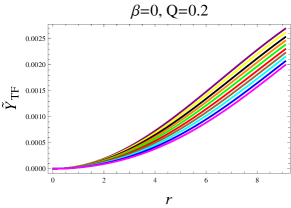
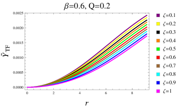
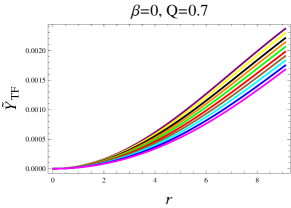
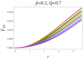
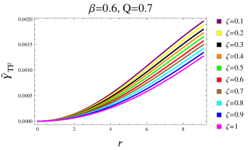
Figure 6: Complexity factor (61).

5.1 Additional Fluid Setup admitting Null Complexity

Here, we consider the scenario that adding the new fluid source makes no change in the complexity of initial source, i.e., $Y_{TF}^{\Theta}=0$. In other words, the complexity of initial and total matter distribution are same. This is mathematically defined as $\tilde{Y}_{TF}=Y_{TF}$, leads to

$$\Pi_{\Theta}=-\frac{1}{2r^{3}}\int_{0}^{r}\tilde{r}^{3}\Theta{{}_{0}^{0}}^{\prime}(\tilde{r})d\tilde{r}.$$ (62)

Solving the right side of the above equation by using (25), we obtain

$$-\frac{1}{2r^{3}}\int_{0}^{r}\tilde{r}^{3}\Theta{{}_{0}^{0}}^{\prime}(\tilde{r})d\tilde{r}=\frac{d_{f}}{r^{2}}-\frac{{d_{f}}^{\prime}}{2r},$$ (63)

and substituting this back into Eq.(62), the linear-order equation becomes in terms of the differential of a function $d_{f}(r)$ as

$$r{d_{f}}^{\prime}(r)\big{(}r\sigma^{\prime}+4\big{)}+d_{f}(r)\big{(}2r^{2}\sigma^{\prime\prime}+r^{2}\sigma^{\prime 2}-2r\sigma^{\prime}-8\big{)}=0.$$ (64)

This single equation contains two unknowns, one deformation function and one metric potential. One can solve it for the former factor only by assuming a known form of the later quantity. We, therefore, adopt the Tolman IV ansatz to solve Eq.(64) expressed by

$$\sigma(r) =\ln\bigg{\{}a_{5}\bigg{(}1+\frac{r^{2}}{a_{4}}\bigg{)}\bigg{\}},$$ (65)

$$\chi(r) =e^{-\alpha}=\frac{\big{(}a_{4}+r^{2}\big{)}\big{(}a_{6}-r^{2}\big{)}}{a_{6}\big{(}a_{4}+2r^{2}\big{)}},$$ (66)

whose corresponding fluid components are

$$\rho =\frac{1}{a_{6}\big{(}a_{4}+2r^{2}\big{)}^{2}}\big{[}a_{4}^{2}\big{(}3-a_{6}r^{2}\omega^{2}-6\beta\big{)}+2r^{2}\big{\{}a_{6}\big{(}2\beta-2r^{4}\omega^{2}+1\big{)}$$

$$+3(1-4\beta)r^{2}\big{\}}+a_{4}\big{\{}a_{6}\big{(}3-4r^{4}\omega^{2}\big{)}+(7-22\beta)r^{2}\big{\}}\big{]},$$ (67)

$$P =\frac{1}{a_{6}\big{(}a_{4}+2r^{2}\big{)}^{2}}\big{[}a_{4}^{2}\big{(}a_{6}r^{2}\omega^{2}+6\beta-1\big{)}+2r^{2}\big{\{}a_{6}\big{(}1-2\beta+2r^{4}\omega^{2}\big{)}$$

$$+3(4\beta-1)r^{2}\big{\}}+a_{4}\big{\{}a_{6}\big{(}4r^{4}\omega^{2}+1\big{)}+(22\beta-5)r^{2}\big{\}}\big{]}.$$ (68)

To find the triplet ($a_{4},a_{5},a_{6}$) appeared in Eqs.(65) and (66), we need to use the Reissner-Nordström metric (36) again. Their expressions in the presence of charge take the form

$$a_{4} =\frac{\mathrm{R}^{2}\big{(}2\mathrm{R}^{2}-6\tilde{M}\mathrm{R}+3\mathrm{Q}^{2}\big{)}}{2\tilde{M}\mathrm{R}-\mathrm{Q}^{2}},$$ (69)

$$a_{5} =\frac{2\mathrm{R}^{2}-6\tilde{M}\mathrm{R}+3\mathrm{Q}^{2}}{2\mathrm{R}^{2}},$$ (70)

$$a_{6} =\frac{2\mathrm{R}^{3}\big{(}\mathrm{Q}^{2}-2\tilde{M}\mathrm{R}+\mathrm{R}^{2}\big{)}}{2\tilde{M}\mathrm{Q}^{2}-4\tilde{M}^{2}\mathrm{R}+\mathrm{Q}^{2}\mathrm{R}+2\tilde{M}\mathrm{R}^{2}}.$$ (71)

We now incorporate the temporal coefficient (65) in Eq.(64) and perform integration to get $d_{f}(r)$ as

$$d_{f}(r)=\frac{c_{2}r^{2}\big{(}a_{4}+r^{2}\big{)}}{2a_{4}+3r^{2}},$$ (72)

with an arbitrary constant $c_{2}$. Joining this with Eq.(18) leads to the modified radial component as

$$e^{\alpha} =\chi^{-1}=\frac{a_{6}\big{(}2a_{4}+3r^{2}\big{)}\big{(}a_{4}+2r^{2}\big{)}}{\big{(}a_{4}+r^{2}\big{)}\big{\{}\big{(}2a_{4}+3r^{2}\big{)}\big{(}a_{6}-r^{2}\big{)}+\zeta c_{2}a_{6}r^{2}\big{(}a_{4}+2r^{2}\big{)}\big{\}}}.$$ (73)

Finally, the complexity factor (57) takes the form for the solution analogous to Eq.(62) by

$$\tilde{Y}_{TF} =Y_{TF}=\frac{1}{80a_{6}r^{3}}\bigg{[}16a_{6}r^{5}\omega^{2}+20(2\beta+1)\big{(}a_{4}+2a_{6}\big{)}r-45\sqrt{2}\beta\sqrt{a_{4}}$$

$$\times\big{(}a_{4}+2a_{6}\big{)}\tan^{-1}\bigg{(}\frac{\sqrt{2}r}{\sqrt{a_{4}}}\bigg{)}+\frac{1}{\big{(}a_{4}+2r^{2}\big{)}^{2}}\big{\{}10(7\beta-4)\big{(}a_{4}+2r^{2}\big{)}a_{4}$$

$$\times\big{(}a_{4}+2a_{6}\big{)}r-20(\beta-1)a_{4}^{2}\big{(}a_{4}+2a_{6}\big{)}r\big{\}}\bigg{]}.$$ (74)

Figure 7 depicts its plots by varying the Rastall parameter and charge, as this is not dependent on $\zeta$. This factor admits an increasing trend w.r.t. $r$, however, decreases by increasing the parameter $\beta$. We also notice that this factor monotonically increases within the range of $0\leq r\leq 8$ and then again decreases in contrast with the one discussed in Figure 6. Further, more the charge is, less complex is the interior and thus indicating the significance of the presence of an electromagnetic field in the study of compact stars.

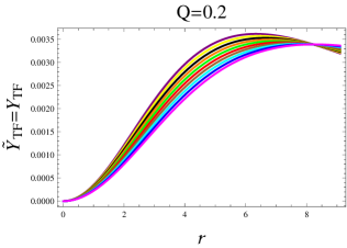
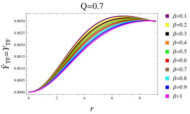
Figure 7: Complexity factor (74).

5.2 Total Fluid Setup admitting Null Complexity

Another constraint we choose in this subsection also depends on the new gravitational source. It is considered that both the initial and extra sources may have complexity totally opposite to each other, i.e., when we add them, the complexity of the total fluid distribution may vanish. This is mathematically expressed as $Y^{\Theta}_{TF}\neq 0$. On the other hand, we can say that the initial source must have the non-null complexity factor, justifying the utilization of the gravitational decoupling strategy that simplifies the complex equations governing the geometry. When we merge this constraint with Eqs.(57), (65) and (66), it becomes

$$40a_{6}r^{2}\big{(}a_{4}+r^{2}\big{)}\big{(}a_{4}+2r^{2}\big{)}{d_{f}}^{\prime}(r)+40a_{6}r\big{(}a_{4}+r^{2}\big{)}^{2}\big{(}r{d_{f}}^{\prime}(r)-2{d_{f}}(r)\big{)}$$

$$-80a_{6}r\big{(}2a_{4}r^{2}+a_{4}^{2}+2r^{4}\big{)}{d_{f}}(r)+\big{(}a_{4}+r^{2}\big{)}^{2}\big{\{}16a_{6}r^{5}\omega^{2}+20(2\beta+1)$$

$$\times\big{(}a_{4}+2a_{6}\big{)}r+\frac{10(7\beta-4)a_{4}\big{(}a_{4}+2a_{6}\big{)}r}{a_{4}+2r^{2}}-\frac{20(\beta-1)a_{4}^{2}\big{(}a_{4}+2a_{6}\big{)}r}{\big{(}a_{4}+2r^{2}\big{)}^{2}}$$

$$-45\sqrt{2}\beta\sqrt{a_{4}}\big{(}a_{4}+2a_{6}\big{)}\tan^{-1}\big{(}\tau_{3}\big{)}\big{\}}=0,$$ (75)

where $\tau_{3}=\frac{\sqrt{2}r}{\sqrt{a_{4}}}$. Working out the solution of the above equation for $d_{f}(r)$, we get the following expression containing $c_{3}$ as a constant

$$d_{f}(r) =\frac{c_{3}r^{2}\big{(}a_{4}+r^{2}\big{)}}{2a_{4}+3r^{2}}-\frac{a_{4}+r^{2}}{40a_{6}r\big{(}a_{4}+2r^{2}\big{)}\big{(}2a_{4}+3r^{2}\big{)}}\big{\{}30\beta r\big{(}a_{4}+2a_{6}\big{)}$$

$$\times\big{(}a_{4}+2r^{2}\big{)}-20(\beta-1)\big{(}a_{4}+2a_{6}\big{)}r^{3}-8a_{6}r^{5}\omega^{2}\big{(}a_{4}+2r^{2}\big{)}$$

$$-15\sqrt{2}\beta\sqrt{a_{4}}\big{(}a_{4}+2a_{6}\big{)}\big{(}a_{4}+2r^{2}\big{)}\tan^{-1}\big{(}\tau_{3}\big{)}\big{\}},$$ (76)

where $\mathrm{Dim}(c_{3})=\frac{1}{\ell^{2}}$. We now use this with Eq.(18) to get modified radial component of the interior geometry as

$$e^{\alpha}=\chi^{-1} =\frac{40a_{6}r\big{(}a_{4}+2r^{2}\big{)}\big{(}2a_{4}+3r^{2}\big{)}}{a_{4}+r^{2}}\bigg{[}15\sqrt{2}\beta a_{4}^{5/2}\zeta\tan^{-1}\big{(}\tau_{3}\big{)}+4a_{4}r\big{\{}a_{6}$$

$$\times\big{(}10c_{3}\zeta r^{2}-15\beta\zeta+2\zeta r^{4}\omega^{2}+20\big{)}-5r^{2}(2\beta\zeta+\zeta+4)\big{\}}+8a_{6}r^{3}$$

$$\times\big{\{}10c_{3}\zeta r^{2}+\zeta\big{(}2r^{4}\omega^{2}-10\beta-5\big{)}+15\big{\}}-30\beta a_{4}^{2}\zeta r-120r^{5}+60$$

$$\times\sqrt{2}\beta\sqrt{a_{4}}a_{6}\zeta r^{2}\tan^{-1}\big{(}\tau_{3}\big{)}+30\sqrt{2}\beta a_{4}^{3/2}\zeta\big{(}a_{6}+r^{2}\big{)}\tan^{-1}\big{(}\tau_{3}\big{)}\bigg{]}^{-1}.$$ (77)

This completes our minimally deformed solution analogous to the constraint $\tilde{Y}_{TF}\neq 0$. Finally, one can find the triplet of fluid variables using Eqs.(28) and (77). They are presented in Appendix A.

The matter triplet (A1)-(A3) representing spherical interior and its corresponding physical characteristics are now interpreted through graphical representation. We again use the same parametric variations as described earlier for the solution corresponding to $\tilde{\Pi}=0$. Nonetheless, the constant $c_{3}$ is differently adopted as $c_{3}=-0.045$. We firstly display the extended $g_{rr}$ potential (77) in Figure 8 whose minimum value is 1 and maximum value varies when altering the Rastall and decoupling parameters along with charge. Figures 9 and 10 depict the matter triplet and anisotropy, and one can easily observe variations in these factors w.r.t. the radial coordinate and all other parameters. They are consistent with the desired behavior, and thus with the first developed model as well. The numerical values of the mass function for certain parametric choices as $\beta=0.6$ and $\zeta=0.1$ are $\tilde{M}=1.632M_{\bigodot}$ and $1.592M_{\bigodot}$ for $Q=0.2$ and $0.7$, respectively. However, the best fit mass with the observed data is found for lower choices of the decoupling parameter and higher values of the charge. The increasing anisotropy (depicted in last rows of both Figures) also guarantees the physical acceptability of this model. The energy conditions which are necessary to be checked in such scenarios are explored without adding their plots, indicating the existence of usual fluid and viability of the solution (A1)-(A3). We eventually check the stability in Figures 11 and 12, and reach at the conclusion that all plots are consistent with the required criteria, leading our model to be stable.

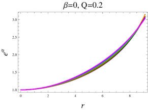
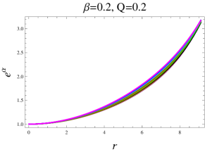
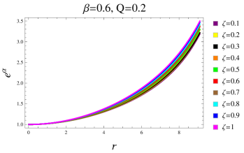
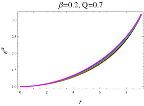
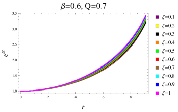
Figure 8: Radial metric (77).

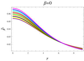
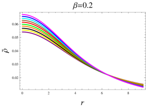
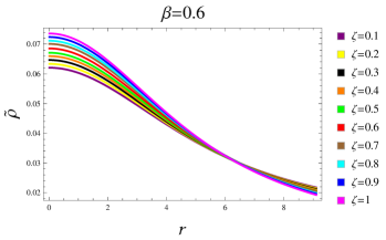
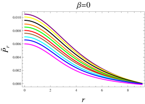
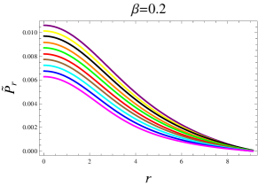
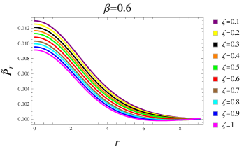
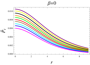
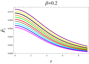
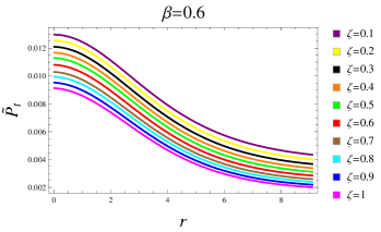
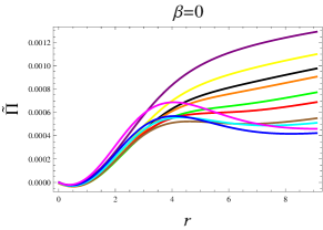
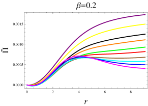
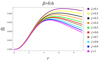
Figure 9: Matter variables corresponding to $\mathrm{Q}=0.2$.

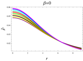
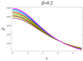
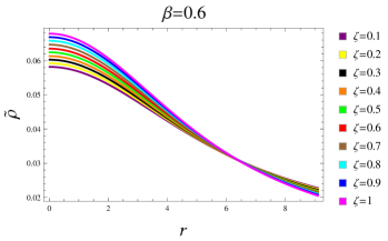
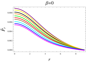
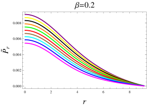
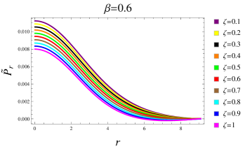
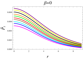
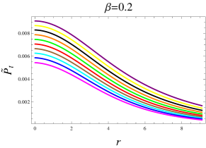
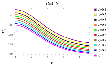
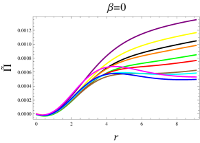
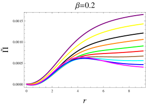
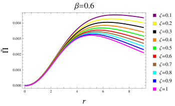
Figure 10: Matter variables corresponding to $\mathrm{Q}=0.7$.

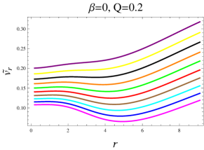
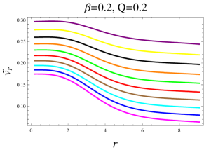
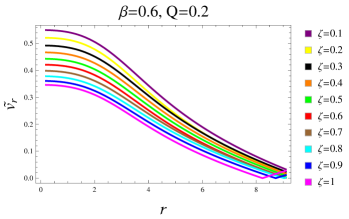
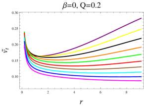
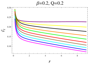
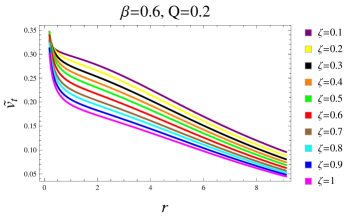
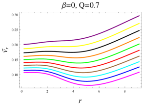
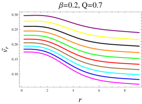
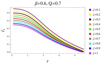
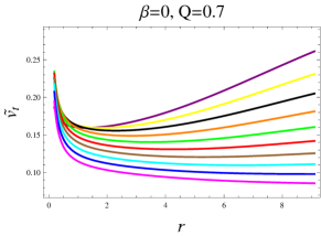
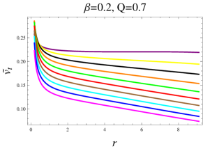
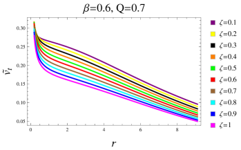
Figure 11: Sound speeds in radial and tangential directions.

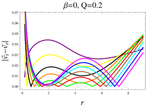
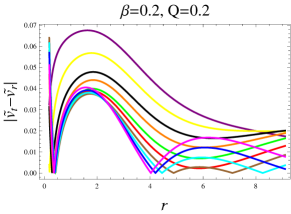
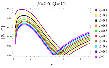
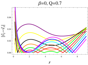
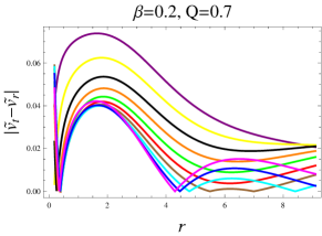
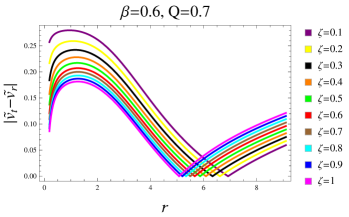
Figure 12: Herrera’s cracking criteria.

6 Conclusions

In this article, I have examined the established methodologies within GR and applied them in the context of Rastall gravity theory. This investigation commenced by adopting a charged static anisotropic spherical interior and modifying it through the incorporation of an additional source. This inclusion resulted in a heightened intricacy within the Rastall gravitational equations, and thus, to streamline and simplify them, I have employed the MGD scheme. This method involved segregating the equations into separate sets that describe specific fluid configurations. To work out the field equations for an initial anisotropic fluid arrangement, two distinct ansatz have been employed. These assumptions pertains to the Krori-Barua spacetime configuration, which is defined by

$$\sigma(r)=a_{1}r^{2}+a_{2},\quad\chi(r)=e^{-\alpha(r)}=e^{-a_{3}r^{2}},$$

while the second model being Tolman IV metric potentials are provided as follows

$$\sigma(r)=\ln\bigg{\{}a_{5}\bigg{(}1+\frac{r^{2}}{a_{4}}\bigg{)}\bigg{\}},\quad\chi(r)=e^{-\alpha(r)}=\frac{\big{(}a_{4}+r^{2}\big{)}\big{(}a_{6}-r^{2}\big{)}}{a_{6}\big{(}a_{4}+2r^{2}\big{)}}.$$

The triplet in each spacetime ansatz has been calculated using the matching conditions at the interface. To achieve this, I utilized observed radius and mass of a compact object, specifically $4U1820-30$. It has also been observed that certain constants possess distinct dimensions, while others are dimensionless. Furthermore, the system represented by Eqs.(25)-(27) contained four unknowns, necessitating the imposition of a single constraint on the matter source $\Theta_{\eta\mu}$ at a time to get a solution. Three distinct models have been formulated, each corresponding to a specific constraint applied to the system as follows

• A mathematical isotropization of the anisotropic compact matter setup, i.e., $\tilde{\Pi}=0$ only for a specific value of $\zeta$,

• Vanishing complexity factor corresponding to extra matter setup, i.e., $Y_{TF}^{\Theta}=0$,

• Vanishing complexity factor corresponding to total matter setup, i.e., $\tilde{Y}_{TF}=0$.

Subsequent to this, I have graphically analyzed the two models corresponding to first and third constraints given above using different Rastall, decoupling and charge parametric values. For instance, I have adopted $\beta=0.2,0.6$, $\zeta=0.1,~0.2,~...~,1$ and $\mathrm{Q}=0.2,0.7$ to plot essential properties for the formulated solutions. The corresponding modified radial metric potential, effective form of fluid variables along with their anisotropic factors have been assessed and found consistent with the required behavior. It has further been observed that the decrement in Rastall parameter and charge makes the interior more massive in all cases. Afterwards, I have successfully displayed some graphical plots to find compatibility of developed models with the viability criteria (LABEL:g50), hence, they are composed of usual fluid. Also, the interior geometry for the second model possesses more mass as compared to the first one for all choices of $\beta$ and $\zeta$. Two complexity factors have been obtained in Eqs.(61) and (74), and plotted, showing increasing behavior outwards, as can be confirmed from Figures 5 and 6. Finally, for the stability check, I have used two techniques depending on the sound speed. It has been confirmed that all these criteria produced stable and physically existing models for all selected values of $\zeta$, $\beta$ and charge. They are found to be consistent with their analogues in GR [61]. It is also important to discuss here that I find more interesting results in Rastall framework when comparing them with the Brans-Dicke [63] and minimally coupled $f(R,T)$ theory [98]. This is because the first solution is stable for all parametric values only in the current setup. Extend this work to include non-linear equations of state and examining the effects of dark energy in future could further enrich our understanding of cosmic evolution under non-conserved gravity theories. Investigating the interplay between Rastall gravity and other alternative theories may also unveil new avenues for addressing current cosmological challenges, such as the $H_{0}$ tension and dark matter interactions. Finally, these results shall be reduced in GR after substituting $\beta=0$.

Appendix A

The fluid parameters analogous to the constraint $\tilde{Y}_{TF}\neq 0$ are

$$\tilde{\rho} =\frac{1}{a_{6}\big{(}a_{4}+2r^{2}\big{)}^{2}}\big{\{}2a_{6}r^{2}\big{(}2\beta-2r^{4}\omega^{2}+1\big{)}-a_{4}^{2}\big{(}a_{6}r^{2}\omega^{2}+6\beta-3\big{)}+a_{4}\big{(}a_{6}$$

$$\times\big{(}3-4r^{4}\omega^{2}\big{)}+(7-22\beta)r^{2}\big{)}+6(1-4\beta)r^{4}\big{\}}-\frac{\zeta(2a_{4}r+3r^{3})^{-2}}{40a_{6}(\tau_{3}^{2}+1)\big{(}a_{4}+2r^{2}\big{)}^{2}}$$

$$\times\big{[}4a_{4}^{2}r^{4}\big{(}\tau_{3}^{2}+1\big{)}\big{\{}a_{6}\big{(}850c_{3}r^{2}-175\beta+294r^{4}\omega^{2}-170\big{)}-15(7\beta+5)r^{2}\big{\}}$$

$$+2a_{4}^{3}r^{2}\big{(}\tau_{3}^{2}+1\big{)}\big{\{}a_{6}\big{(}740c_{3}r^{2}-210\beta+252r^{4}\omega^{2}-120\big{)}-5(35\beta+34)r^{2}\big{\}}$$

$$+10a_{4}^{4}\big{(}\tau_{3}^{2}+1\big{)}\big{\{}4a_{6}\big{(}6c_{3}r^{2}-3\beta+2r^{4}\omega^{2}\big{)}-3(7\beta+4)r^{2}\big{\}}+240\big{(}\tau_{3}^{2}+1\big{)}$$

$$\times a_{6}r^{8}\big{(}6c_{3}r^{2}-2\beta+2r^{4}\omega^{2}-1\big{)}+8a_{4}r^{6}\big{(}\tau_{3}^{2}+1\big{)}\big{\{}a_{6}\big{(}440c_{3}r^{2}-105\beta+r^{4}$$

$$\times 152\omega^{2}-75\big{)}-15(2\beta+1)r^{2}\big{\}}+360\sqrt{2}\beta\sqrt{a_{4}}a_{6}r^{8}\tau_{3}^{\prime}+15\sqrt{2}\beta a_{4}^{7/2}r\big{\{}\big{(}26a_{6}$$

$$+31r^{2}\big{)}r\tau_{3}^{\prime}-4\big{(}a_{6}+2r^{2}\big{)}\big{(}\tau_{3}^{2}+1\big{)}\tan^{-1}\big{(}\tau_{3}\big{)}\big{\}}+15\sqrt{2}\beta a_{4}^{9/2}\big{\{}\big{(}4a_{6}+13r^{2}\big{)}$$

$$\times\tau_{3}^{\prime}-2r\big{(}\tau_{3}^{2}+1\big{)}\tan^{-1}\big{(}\tau_{3}\big{)}\big{\}}+60\sqrt{2}\beta a_{4}^{3/2}r^{5}\big{\{}r\big{(}16a_{6}+3r^{2}\big{)}\tau_{3}^{\prime}-\big{(}\tau_{3}^{2}+1\big{)}$$

$$\times 4a_{6}\tan^{-1}\big{(}\tau_{3}\big{)}\big{\}}+30\sqrt{2}\beta a_{4}^{5/2}r^{3}\big{\{}r\big{(}31a_{6}+16r^{2}\big{)}\tau_{3}^{\prime}-4\big{(}2a_{6}+r^{2}\big{)}\big{(}\tau_{3}^{2}+1\big{)}$$

$$\times\tan^{-1}\big{(}\tau_{3}\big{)}\big{\}}+30\sqrt{2}\beta a_{4}^{11/2}\tau_{3}^{\prime}-60\beta a_{4}^{5}\big{(}\tau_{3}^{2}+1\big{)}\big{]},$$ (A1)

$$\tilde{P}_{r} =\frac{1}{a_{6}\big{(}a_{4}+2r^{2}\big{)}^{2}}\big{[}a_{4}^{2}\big{(}a_{6}r^{2}\omega^{2}+6\beta-1\big{)}+2r^{2}\big{\{}a_{6}\big{(}1-2\beta+2r^{4}\omega^{2}\big{)}+3r^{2}$$

$$\times(4\beta-1)\big{\}}+a_{4}\big{\{}a_{6}\big{(}4r^{4}\omega^{2}+1\big{)}+(22\beta-5)r^{2}\big{\}}\big{]}+\frac{\zeta\big{(}3r^{2}+a_{4}\big{)}}{r^{2}+a_{4}}\bigg{[}c_{3}r^{2}$$

$$\times\frac{\big{(}a_{4}+r^{2}\big{)}}{2a_{4}+3r^{2}}-\frac{a_{4}+r^{2}}{40a_{6}r\big{(}a_{4}+2r^{2}\big{)}\big{(}2a_{4}+3r^{2}\big{)}}\big{\{}30\beta r\big{(}a_{4}+2a_{6}\big{)}\big{(}a_{4}+2r^{2}\big{)}$$

$$-20(\beta-1)\big{(}a_{4}+2a_{6}\big{)}r^{3}-8a_{6}r^{5}\omega^{2}\big{(}a_{4}+2r^{2}\big{)}-15\big{(}a_{4}+2a_{6}\big{)}\big{(}a_{4}+2r^{2}\big{)}$$

$$\times\sqrt{2}\beta\sqrt{a_{4}}\tan^{-1}\big{(}\tau_{3}\big{)}\big{\}}\bigg{]},$$ (A2)

$$\tilde{P}_{t} =\frac{1}{a_{6}\big{(}a_{4}+2r^{2}\big{)}^{2}}\big{[}a_{4}^{2}\big{(}a_{6}r^{2}\omega^{2}+6\beta-1\big{)}+2r^{2}\big{\{}a_{6}\big{(}1-2\beta+2r^{4}\omega^{2}\big{)}+3r^{2}$$

$$\times(4\beta-1)\big{\}}+a_{4}\big{\{}a_{6}\big{(}4r^{4}\omega^{2}+1\big{)}+(22\beta-5)r^{2}\big{\}}\big{]}+\frac{\zeta}{80a_{6}r^{3}(2a_{4}+3r^{2})^{2}}$$

$$\times\frac{1}{(a_{4}+r^{2})(a_{4}+2r^{2})^{2}}\big{[}4a_{4}^{4}r^{3}\big{\{}2a_{6}\big{(}20c_{3}(9r+4)r-25\beta+66r^{4}\omega^{2}+32r^{3}\omega^{2}$$

$$-20\big{)}-5r((37\beta+20)r-28\beta+16)\big{\}}+4a_{4}^{5}r^{3}\big{\{}8a_{6}\big{(}5c_{3}+2r^{2}\omega^{2}\big{)}-(5\beta+4)$$

$$\times 5\big{\}}+96a_{6}r^{11}\big{\{}-10\beta+20c_{3}(r+2)r+6r^{4}\omega^{2}+16r^{3}\omega^{2}-5\big{\}}+4a_{4}^{3}r^{4}\big{\{}2a_{6}$$

$$\times\big{(}20(7\beta-4)+30c_{3}(21r+16)r^{2}+214r^{5}\omega^{2}+200r^{4}\omega^{2}-5(37\beta+20)r\big{)}$$

$$-5r^{2}((87\beta+42)r-80\beta+32)\big{\}}+8a_{4}^{2}r^{6}\big{\{}a_{6}\big{(}80(5\beta-2)+20c_{3}(53r+54)$$

$$\times r^{2}+338r^{5}\omega^{2}+464r^{4}\omega^{2}-15(29\beta+14)r\big{)}-20r^{2}(5(2\beta+1)r-7\beta+1)\big{\}}$$

$$+16a_{4}r^{8}\big{\{}4a_{6}\big{(}35\beta+35c_{3}(3r+4)r^{2}+32r^{5}\omega^{2}+60r^{4}\omega^{2}-25(2\beta+1)r-5\big{)}$$

$$-15(2\beta+1)r^{3}\big{\}}+360\sqrt{2}\beta\sqrt{a_{4}}a_{6}r^{9}\big{(}r(r+4)\tau_{4}^{\prime}+(r-4)\tau_{4}\big{)}+30\sqrt{2}\beta a_{4}^{9/2}r$$

$$\times\big{\{}r\big{(}a_{6}(15r+8)+2(11r+13)r^{2}\big{)}\tau_{4}^{\prime}-\big{(}a_{6}(9r+8)+3(r+10)r^{2}\big{)}\tau_{4}\big{\}}+60$$

$$\times\sqrt{2}\beta a_{4}^{3/2}r^{7}\big{\{}r\big{(}a_{6}(22r+64)+3(r+4)r^{2}\big{)}\tau_{4}^{\prime}+\big{(}2a_{6}(9r-40)+3(r-4)r^{2}\big{)}$$

$$\times\tau_{4}\big{\}}+30\sqrt{2}\beta a_{4}^{5/2}r^{5}\big{\{}r\big{(}a_{6}(63r+124)+2(11r+32)r^{2}\big{)}\tau_{4}^{\prime}+\big{(}(23r-156)$$

$$\times a_{6}+2(9r-40)r^{2}\big{)}\tau_{4}\big{\}}+15\sqrt{2}\beta a_{4}^{7/2}r^{3}\big{\{}r\big{(}8a_{6}(11r+13)+(63r+124)r^{2}\big{)}$$

$$\times\tau_{4}^{\prime}+\big{(}r^{2}(23r-156)-12a_{6}(r+10)\big{)}\tau_{4}\big{\}}-30\sqrt{2}\beta a_{4}^{13/2}\big{(}\tau_{4}-r\tau_{4}^{\prime}\big{)}+15\beta$$

$$\times\sqrt{2}a_{4}^{11/2}\big{\{}r\big{(}4a_{6}+r(15r+8)\big{)}\tau_{4}^{\prime}-\big{(}4a_{6}+r(9r+8)\big{)}\tau_{4}\big{\}}\big{]},$$ (A3)

where $\tau_{4}=\tan^{-1}(\tau_{3})$. Moreover, the last two equations expressed above are used to find the corresponding anisotropy as

$$\tilde{\Pi} =\frac{\zeta}{80a_{6}r^{3}(a_{4}+r^{2})(a_{4}+2r^{2})^{2}(2a_{4}+3r^{2})^{2}}\big{[}4a_{4}^{4}r^{3}\big{\{}2a_{6}\big{(}20c_{3}(9r+4)r-25\beta$$

$$+66r^{4}\omega^{2}+32r^{3}\omega^{2}-20\big{)}-5r((37\beta+20)r-28\beta+16)\big{\}}+4a_{4}^{5}r^{3}\big{\{}8a_{6}\big{(}5c_{3}$$

$$+2r^{2}\omega^{2}\big{)}-(5\beta+4)5\big{\}}+96a_{6}r^{11}\big{\{}-10\beta+20c_{3}(r+2)r+6r^{4}\omega^{2}+16r^{3}\omega^{2}$$

$$-5\big{\}}+4a_{4}^{3}r^{4}\big{\{}2a_{6}\big{(}20(7\beta-4)+30c_{3}(21r+16)r^{2}+214r^{5}\omega^{2}+200r^{4}\omega^{2}-5$$

$$\times(37\beta+20)r\big{)}-5r^{2}((87\beta+42)r-80\beta+32)\big{\}}+8a_{4}^{2}r^{6}\big{\{}a_{6}\big{(}20c_{3}(53r+54)$$

$$+80(5\beta-2)r^{2}+338r^{5}\omega^{2}+464r^{4}\omega^{2}-15(29\beta+14)r\big{)}-20r^{2}(5(2\beta+1)r$$

$$-7\beta+1)\big{\}}+16a_{4}r^{8}\big{\{}4a_{6}\big{(}35\beta+35c_{3}(3r+4)r^{2}+32r^{5}\omega^{2}+60r^{4}\omega^{2}-25r$$

$$\times(2\beta+1)-5\big{)}-15(2\beta+1)r^{3}\big{\}}+360\sqrt{2}\beta\sqrt{a_{4}}a_{6}r^{9}\big{(}r(r+4)\tau_{4}^{\prime}+(r-4)\tau_{4}\big{)}$$

$$+30\sqrt{2}\beta a_{4}^{9/2}r\big{\{}r\big{(}a_{6}(15r+8)+2(11r+13)r^{2}\big{)}\tau_{4}^{\prime}-\big{(}a_{6}(9r+8)+3(r+10)$$

$$\times r^{2}\big{)}\tau_{4}\big{\}}+60\sqrt{2}\beta a_{4}^{3/2}r^{7}\big{\{}r\big{(}a_{6}(22r+64)+3(r+4)r^{2}\big{)}\tau_{4}^{\prime}+\big{(}2a_{6}(9r-40)$$

$$+3(r-4)r^{2}\big{)}\tau_{4}\big{\}}+30\sqrt{2}\beta a_{4}^{5/2}r^{5}\big{\{}r\big{(}a_{6}(63r+124)+2(11r+32)r^{2}\big{)}\tau_{4}^{\prime}+\big{(}a_{6}$$

$$\times(23r-156)+2(9r-40)r^{2}\big{)}\tau_{4}\big{\}}+15\sqrt{2}\beta a_{4}^{7/2}r^{3}\big{\{}r\big{(}8a_{6}(11r+13)+(63r$$

$$+124)r^{2}\big{)}\tau_{4}^{\prime}+\big{(}r^{2}(23r-156)-12a_{6}(r+10)\big{)}\tau_{4}\big{\}}-30\sqrt{2}\beta a_{4}^{13/2}\big{(}\tau_{4}-r\tau_{4}^{\prime}\big{)}$$

$$+15\sqrt{2}a_{4}^{11/2}\beta\big{\{}r\big{(}4a_{6}+r(15r+8)\big{)}\tau_{4}^{\prime}-\big{(}4a_{6}+r(9r+8)\big{)}\tau_{4}\big{\}}\big{]}-\frac{\zeta\big{(}3r^{2}+a_{4}\big{)}}{r^{2}+a_{4}}$$

$$\times\bigg{[}\frac{c_{3}r^{2}\big{(}a_{4}+r^{2}\big{)}}{2a_{4}+3r^{2}}-\frac{a_{4}+r^{2}}{40a_{6}r\big{(}a_{4}+2r^{2}\big{)}\big{(}2a_{4}+3r^{2}\big{)}}\big{\{}30\beta r\big{(}a_{4}+2a_{6}\big{)}\big{(}a_{4}+2r^{2}\big{)}$$

$$-20(\beta-1)\big{(}a_{4}+2a_{6}\big{)}r^{3}-8a_{6}r^{5}\omega^{2}\big{(}a_{4}+2r^{2}\big{)}-15\big{(}a_{4}+2a_{6}\big{)}\big{(}a_{4}+2r^{2}\big{)}$$

$$\times\sqrt{2}\beta\sqrt{a_{4}}\tan^{-1}\big{(}\tau_{3}\big{)}\big{\}}\bigg{]}.$$ (A4)

References

- [1] Ratall, P.: Phys. Rev. D 6(1972)3357.
- [2] Heydarzade, Y. and Darabi, F.: Phys. Lett. B 771(2017)365.
- [3] Licata, I., Moradpour, H. and Corda, C.: Int. J. Geom. Methods Mod. Phys. 14(2017)1730003.
- [4] Xu, Z., Hou, X., Gong, X. and Wang, J.: Eur. Phys. J. C 78(2018)01.
- [5] Graca, J.M. and Lobo, I.P.: Eur. Phys. J. C 78(2018)101.
- [6] Kumar, R. and Ghosh, S.G.: Eur. Phys. J. C. 78(2018)750;
- [7] Darabi, F., Atazadeh, K. and Heydarzade, Y.: Eur. Phys. J. Plus 133(2018)249.
- [8] Haghani, Z., Harko, T. and Shahidi, S.: Phys. Dark Universe 21(2018)27.
- [9] Visser, M.: Phys. Lett. B 782(2018)83.
- [10] Maurya, S.K. and Tello-Ortiz, F.: Phys. Dark Universe 29(2020)100577.
- [11] Mustafa, G., Hussain, I., Shamir, M.F. and Tie-Cheng, X.: Phys. Scr. 96(2021)045009.
- [12] Naseer, T.: Phys. Dark Universe 46(2024)101663.
- [13] Sharif, M., Naseer, T. and Tabassum, A.: Chin. J. Phys. 92(2024)579.
- [14] Naseer, T. and Sharif, M.: Class. Quantum Grav. 41(2024)245006.
- [15] Batista, C.E.M. et al.: Eur. Phys. J. C 73(2013)2425.
- [16] Fabris, J.C. et al.: AIP Conf. Proc. 1647(2015)50.
- [17] Darabi, F. et al.: Eur. Phys. J. C 78(2018)25.
- [18] Abbas, G. and Shahzad, M.R.: Astrophys. Space Sci. 363(2018)251.
- [19] Abbas, G., Tahir, M. and Shahzad, M.R.: Int. J. Geom. Methods Mod. Phys. 18(2021)2150042.
- [20] Mustafa, G., Tie-Cheng, X. and Shamir, M.F.: Phys. Scr. 96(2021)105008.
- [21] Mota, C.E. et al.: Phys. Scr. 39(2022)085008.
- [22] Nashed, G.G.L.: Nucl. Phys. B 994(2023)116305.
- [23] Pretel, J.M.Z. and Mota, C.E.: Gen. Relativ. Gravit. 56(2024)43.
- [24] Errehymy, A., Daoud, M. and Jammari, M.K.: Eur. Phys. J. Plus 132(2017)497.
- [25] Maurya, S.K., Singh, K.N. and Errehymy, A.: Eur. Phys. J. Plus 137(2022)640.
- [26] Sharif, M. and Naseer, T.: Pramana 96(2022)119.
- [27] Errehymy, A., Khedif, Y., Mustafa, G. and Daoud, M.: Chin. J. Phys. 77(2022)1502.
- [28] Sharif, M. and Naseer, T.: Indian J. Phys. 97(2023)2853.
- [29] Mustafa, G. et al.: Chin. J. Phys. 77(2022)1742.
- [30] Naseer, T. and Sharif, M.: Phys. Dark Universe 46(2024)101595.
- [31] Ovalle, J.: Phys. Rev. D 95(2017)104019.
- [32] Ovalle, J.: Phys. Lett. B 788(2019)213.
- [33] Casadio, R., Ovalle, J. and Da Rocha, R.: Class. Quantum Grav. 32(2015)215020.
- [34] Ovalle, J. et al.: Eur. Phys. J. C 78(2018)960.
- [35] Sharif, M. and Sadiq, S.: Eur. Phys. J. C 78(2018)410.
- [36] Graterol, R.P.: Eur. Phys. J. Plus 133(2018)244.
- [37] Maurya, S.K., Mustafa, G., Govender, M. and Singh, K.N.: J. Cosmol. Astropart. Phys. 10(2022)003.
- [38] Smitha, T.T., Maurya, S.K., Dayanandan, B. and Mustafa, G.: Results Phys. 49(2023)106502.
- [39] Gabbanelli, L., Rincón, Á. and Rubio, C.: Eur. Phys. J. C 78(2018)370.
- [40] Estrada, M. and Tello-Ortiz, F.: Eur. Phys. J. Plus 133(2018)453.
- [41] Hensh, S. and Stuchlík, Z.: Eur. Phys. J. C 79(2019)834.
- [42] Sharif, M. and Naseer, T.: Class. Quantum Grav. 40(2023)035009.
- [43] Naseer, T. and Sharif, M.: Fortschr. Phys. 71(2023)2300004.
- [44] Maurya, S.K. et al.: Fortschr. Phys. 70(2022)2200041.
- [45] Smitha, T.T. et al.: Results Phys. 49(2023)106502.
- [46] Sharif, M. and Naseer, T.: Gen. Relativ. Gravit. 55(2023)87.
- [47] Maurya, S.K. et al.: Phys. Dark Universe 42(2023)101284.
- [48] Sharif, M. and Naseer, T.: Chin. J. Phys. 86(2023)596.
- [49] Feng, Y. et al.: Phys. Scr. 99(2024)085034.
- [50] Naseer, T. and Sharif, M.: Commun. Theor. Phys. 76(2024)095407.
- [51] Tello-Ortiz, F.: Phys. Dark Universe 44(2024)101460.
- [52] Herrera, L.: Phys. Rev. D 97(2018)044010.
- [53] Herrera, L., Di Prisco, A. and Ospino, J.: Phys. Rev. D 98(2018)104059.
- [54] Yousaf, Z. et al.: Mon. Not. R. Astron. Soc. 495(2020)4334.
- [55] Yousaf, Z., Bhatti, M.Z. and Naseer, T.: Ann. Phys. 420(2020)168267.
- [56] Yousaf, Z. et al.: Phys. Dark Universe 29(2020)100581
- [57] Yousaf, Z., Bhatti, M.Z. and Naseer, T.: Phys. Dark Universe 28(2020)100535.
- [58] Carrasco-Hidalgo, M. and Contreras, E.: Eur. Phys. J. C 81(2021)757.
- [59] Andrade, J. and Contreras, E.: Eur. Phys. J. C 81(2021)889.
- [60] Arias, C. et al.: Ann. Phys. 436(2022)168671.
- [61] Casadio, R. et al.: Eur. Phys. J. C 79(2019)826.
- [62] Maurya, S.K. and Nag, R.: Eur. Phys. J. C 82(2022)48.
- [63] Sharif, M. and Majid, A.: Eur. Phys. J. Plus 137(2022)114.
- [64] Roupas, Z. and Nashed, G.G.L.: Eur. Phys. J. C 80(2020)905.
- [65] Biswas, S., Deb, D., Ray, S. and Guha B.K.: Ann. Phys. 428(2021)168429.
- [66] Mohanty, D. and Sahoo, P.K.: Fortschr. Phys. 72(2024)2400082.
- [67] Bhar, P., Singh, K.N., Maurya, S.K. and Govender, M.: Phys. Dark Universe 43(2024)101391.
- [68] Estevez-Delgado, G. et al.: Eur. Phys. J. Plus 135(2020)143.
- [69] Dayanandan, B. and Smitha, T.T.: Chin. J. Phys. 71(2021)683.
- [70] Andrade, J., Fuenmayor, E. and Contreras, E.: Int. J. Mod. Phys. D 31(2022)2250093.
- [71] Errehymy, A. et al.: New Astron. 99(2023)101957.
- [72] Schwarz, D.J. and Weinhorst, B.: Astron. Astrophys. 474(2007)717.
- [73] Antoniou, I. and Perivolaropoulos, L.: J. Cosmol. Astropart. Phys. 12(2010)012.
- [74] Tiwari, P. and Nusser, A.: J. Cosmol. Astropart. Phys. 3(2016)062.
- [75] Řípa, J. and Shafieloo, A.: Astrophys. J. 851(2017)15.
- [76] Migkas, K. and Reiprich, T.H.: Astron. Astrophys. 611(2018)A50.
- [77] Hassan, K., Naseer, T. and Sharif, M.: Chin. J. Phys. 91(2024)916.
- [78] Naseer, T. and Said, J.L.: Eur. Phys. J. C 84(2024)808.
- [79] de Felice, F., Yu, Y.Q. and Fang, J.: Mon. Not. R. Astron. Soc. 277(1995)L17.
- [80] Krori, K.D. and Barua, J.: J. Phys. A: Math. Gen. 8(1975)508.
- [81] Bhar, P.: Astrophys. Space Sci. 356(2015)365.
- [82] Shamir, M.F., Asghar, Z. and Malik, A.: Fortschr. Phys. 70(2022)2200134.
- [83] Darmois, G.: Les equations de la gravitation einsteinienne, (1927).
- [84] Güver, T., Wroblewski, P., Camarota, L. and Özel, F.: Astrophys. J. 719(2010)1807.
- [85] Feng, Y. et al.: Chin. J. Phys. 90(2024)372.
- [86] Demir, E. et al.: Chin. J. Phys. 91(2024)299.
- [87] Buchdahl, H.A.: Phys. Rev. 116(1959)1027.
- [88] Ivanov, B.V.: Phys. Rev. D 65(2002)104011.
- [89] Abreu, H., Hernandez, H. and Nunez, L.A.: Class. Quantum Grav. 24(2007)4631.
- [90] Herrera, L.: Phys. Lett. A 165(1992)206.
- [91] Maurya, S.K. et al.: Eur. Phys. J. C 82(2022)1173.
- [92] Maurya, S.K., Singh, K.N., Lohakare, S.V. and Mishra, B.: Fortschr. Phys. 70(2022)2200061.
- [93] Sharif, M. and Naseer, T.: Phys. Scr. 98(2023)115012
- [94] Maurya, S.K. et al.: Eur. Phys. J. C 83(2023)348.
- [95] Sharif, M. and Naseer, T.: Ann. Phys. 459(2023)169527
- [96] Habsi, M.A. et al.: Eur. Phys. J. C 83(2023)286.
- [97] Maurya, S.K. et al.: Phys. Dark Universe 46(2024)101665.
- [98] Sharif, M. and Naseer, T.: Eur. Phys. J. Plus 137(2022)1304.