Generalizable Origin Identification for
Text-Guided Image-to-Image Diffusion Models

Abstract

Text-guided image-to-image diffusion models excel in translating images based on textual prompts, allowing for precise and creative visual modifications. However, such a powerful technique can be misused for spreading misinformation, infringing on copyrights, and evading content tracing. This motivates us to introduce the task of origin IDentification for text-guided Image-to-image Diffusion models (ID²), aiming to retrieve the original image of a given translated query. A straightforward solution to ID² involves training a specialized deep embedding model to extract and compare features from both query and reference images. However, due to visual discrepancy across generations produced by different diffusion models, this similarity-based approach fails when training on images from one model and testing on those from another, limiting its effectiveness in real-world applications. To solve this challenge of the proposed ID² task, we contribute the first dataset and a theoretically guaranteed method, both emphasizing generalizability. The curated dataset, OriPID, contains abundant Origins and guided Prompts, which can be used to train and test potential IDentification models across various diffusion models. In the method section, we first prove the existence of a linear transformation that minimizes the distance between the pre-trained Variational Autoencoder (VAE) embeddings of generated samples and their origins. Subsequently, it is demonstrated that such a simple linear transformation can be generalized across different diffusion models. Experimental results show that the proposed method achieves satisfying generalization performance, significantly surpassing similarity-based methods ($+31.6\%$ mAP), even those with generalization designs.

1 Introduction

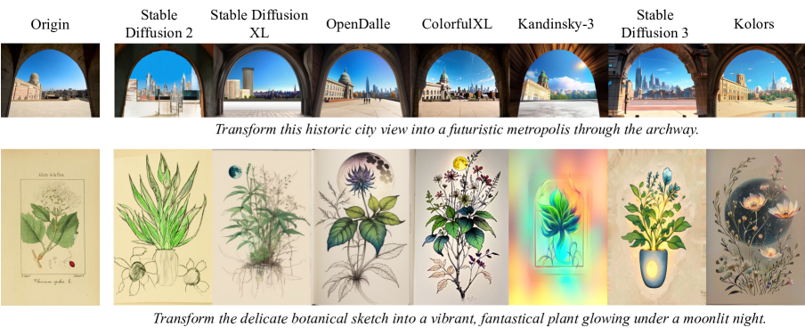
Figure 2: The demonstration for visual discrepancy between generated images by different diffusion models. The images generated by various models exhibit distinctive visual features such as realistic textures, complex architectures, life-like details, vibrant colors, abstract expression, magical ambiance, and photorealistic elements.

Text-guided image-to-image diffusion models are notable for their ability to transform images based on textual descriptions, allowing for detailed and highly customizable modification. While they are increasingly used in creative industries for tasks such as digital art re-creation, customizing visual content, and personalized virtual try-ons, there are growing security concerns associated with their misuse. As illustrated in Fig. 1, for instance, they could be misused for misinformation, copyright infringement, and evading content tracing. To help combat these misuses, this paper introduces the task of origin IDentification for text-guided Image-to-image Diffusion models (ID²), which aims to identify the original image of a generated query from a large-scale reference set. When the origin is identified, subsequent compensations include deploying factual corrections for misinformation, enforcing copyright compliance, and keeping the tracing of target content.

A straightforward solution for the proposed ID² task is to employ a similarity-based retrieval approach. Specifically, this approach (1) fine-tunes a pre-trained network by minimizing the distances between generated images and their origins, and (2) uses the trained network to extract and compare feature vectors from the queries and references. However, this approach is impractical in real-world scenarios. This is because: for most current popular diffusion models, such as Stable Diffusion 2 [36], Stable Diffusion XL [33], OpenDalle [15], ColorfulXL [35], Kandinsky-3 [1], Stable Diffusion 3 [9], and Kolors [17], in a training-free manner, text-guided image-to-image translation can be easily achieved by using an input image with added noise as the starting point (instead of starting from randomly distributed noise). Further, as shown in Fig. 2, there exists a visual discrepancy across images generated by different diffusion models, i.e., different diffusion models exhibit distinct visual features. An experimental evidence for such discrepancy is that we can train a lightweight classification model, such as Swin-S [23], to achieve a top-1 accuracy of 95.9% when classifying images generated by these seven diffusion models. The visual discrepancy presents an inherent challenge of our ID², i.e., the approach mentioned above fails when trained on images generated by one diffusion model and tested on queries from another. For instance, when trained on images generated by Stable Diffusion 2, this approach achieves a 87.1% mAP on queries from Stable Diffusion 2, while only achieving a 30.5% mAP on queries from ColorfulXL.

To address the generalization challenge in the proposed task, our efforts focus primarily on constructing the first ID² dataset and proposing a theoretically guaranteed method.

$\bullet$ A new dataset emphasizing generalization. To verify the generalizability, we construct the first ID² dataset, OriPID, which includes abundant Origins with guided Prompts for training and testing potential IDentification models. Specifically, the training set contains $100,000$ origins. For each origin, we use GPT-4o [26] to generate $20$ different prompts, each of which implies a plausible translation direction. By inputting these origins and prompts into Stable Diffusion 2, we generate $2,000,000$ training images. For testing, we randomly select $5,000$ images as origins from a reference set containing $1,000,000$ images, and ask GPT-4o to generate a guided prompt for each origin. Subsequently, we generate $5,000$ queries using the origins, corresponding prompts, and each of the following models: Stable Diffusion 2, Stable Diffusion XL, OpenDalle, ColorfulXL, Kandinsky-3, Stable Diffusion 3, and Kolors. The design of using different diffusion models to generate training images and queries is particularly practical because, in the real world, where numerous diffusion models are publicly available, we cannot predict which ones might be misused.

$\bullet$ A simple, generalizable, and theoretically guaranteed solution. To solve the generalization problem, we first theoretically prove that, after specific linear transformations, the embeddings of an original image and its translation, encoded by the diffusion model’s Variational Autoencoder (VAE), will be sufficiently close. This suggests that we can use these linearly transformed query embeddings to match against the reference embeddings. Furthermore, we demonstrate that these kinds of feature vectors are generalizable across diffusion models. Specifically, by using a trained linear transformation and the encoder of VAE from one diffusion model, we can also effectively embed the generated images from another diffusion model, even if their VAEs have different parameters or architectures (see Section 5.3 for more details). The effectiveness means the similar performance of origin identification for both diffusion models. Finally, we implement this theory (obtain the expected linear transformation) by gradient descending a metric learning loss and experimentally show the effectiveness and generalizability of the proposed solution.

In summary, we make the following contributions:

1. This paper proposes a novel task, origin identification for text-guided image-to-image diffusion models (ID²), which aims to identify the origin of a generated query. This task tries to alleviate an important and timely security concern, i.e., the misuse of text-guided image-to-image diffusion models. To support this task, we build the first ID² dataset.

2. We highlight an inherent challenge of ID², i.e., the existing visual discrepancy prevents similarity-based methods from generalizing to queries from unknown diffusion models. Therefore, we propose a simple but generalizable method by utilizing linear-transformed embeddings encoded by the VAE. Theoretically, we prove the existence and generalizability of the required linear transformation.

3. Extensive experimental results demonstrate (1) the challenge of the proposed ID² task: all pre-trained deep embedding models, fine-tuned similarity-based methods, and specialized domain generalization methods fail to achieve satisfying performance; and (2) the effectiveness of our proposed method: it achieves $88.8\%$, $81.5\%$, $87.3\%$, $89.3\%$, $85.7\%$, $85.7\%$, and $90.3\%$ mAP, respectively, for seven different diffusion models.

2 Related Works

Diffusion Models. Recent diffusion models, including Stable Diffusion 2 [36], Stable Diffusion XL [33], OpenDalle [15], ColorfulXL [35], Kandinsky-3 [1], Stable Diffusion 3 [9], and Kolors [17], have brought significant improvements in visual generation. This paper considers using these popular diffusion models for text-guided image-to-image translation in a training-free manner, which is a common and cost-effective approach in the real world.

Security Issues with AI-Generated Content. Recently, generative models have gained significant attention due to their impressive capabilities. However, alongside their advancements, several security concerns have been identified. Prior research has explored various dimensions of these security issues. For instance, [22] focuses on detecting AI-generated multimedia to prevent its associated societal disruption. Additionally, [10] and [3] explore the ethical implications and technical challenges in ensuring the integrity and trustworthiness of AI-generated content. In contrast, while our work also aims to help address the security issues, we specifically focus on a novel perspective: identifying the origin of a given translated image.

Image Copy Detection. The task most similar to our ID² is Image Copy Detection (ICD) [29], which identifies whether a query replicates the content of any reference. Various works focus on different aspects: PE-ICD [44] and AnyPattern [43] build benchmarks and propose solutions emphasizing novel patterns in realistic scenarios; ASL [42] addresses the hard negative challenge; Active Image Indexing [11] explores improving the robustness of ICD; and SSCD [31] leverages self-supervised contrastive learning for ICD. Unlike ICD, which focuses on manually-designed transformations, our ID² aims to find the origin of a query translated by the diffusion model with prompt-guidance.

3 Dataset

To advance research in ID², this section introduces OriPID, the first dataset specifically designed for the proposed task. The source images in OriPID are derived from the DISC21 dataset [29], which is a subset of the real-world multimedia dataset YFCC100M [39]. As a result, OriPID is diverse and comprehensive, encompassing a wide range of subjects found in real-world scenarios. An illustration of the proposed dataset is shown in Fig. 3.

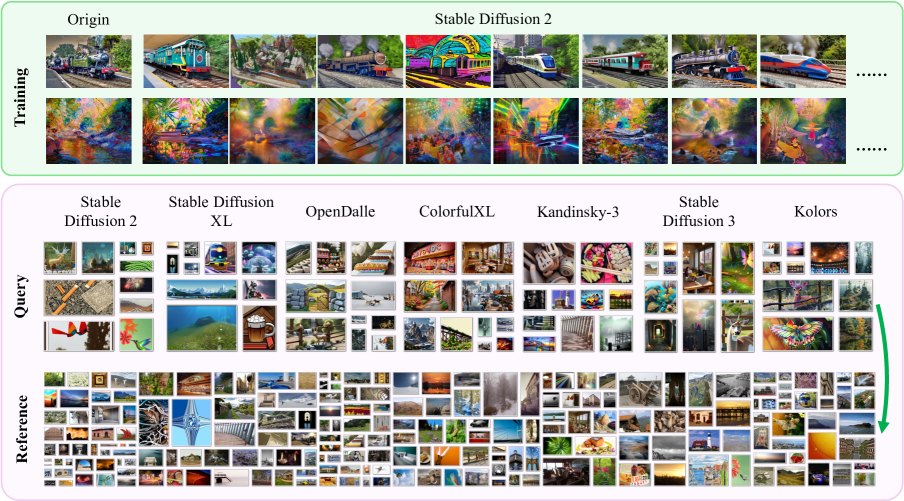
Figure 3: The images in our dataset, which is diverse and comprehensive. Specifically, it encompasses a variety of subjects commonly found in real-world scenarios where issues such as misinformation, copyright infringement, and content tracing evasion occur. For instance, our dataset includes images of nature, architecture, animals, planes, art, and indoor. Note that for simplicity, we omit the prompts here. Please refer to Supplementary (Section 8) for examples of prompts and generations.

Training Set. The training set comprises (1) $100,000$ origins randomly selected from the $1,000,000$ original images in DISC21, (2) $2,000,000$ guided prompts ($20$ for each origin) generated by GPT-4o (for details on how these prompts were generated, see Supplementary (Section 9)), and (3) $2,000,000$ images generated by inputting the origins and prompts into Stable Diffusion 2 [36].

Test Set. We design the test set with a focus on real-world/practical settings. On one hand, we use seven popular diffusion models, namely, Stable Diffusion 2 [36], Stable Diffusion XL [33], OpenDalle [15], ColorfulXL [35], Kandinsky-3 [1], Stable Diffusion 3 [9], and Kolors [17], to generate queries. This setting well simulates real-world scenarios where new diffusion models continuously appear, and we do not know which one is being misused. On the other hand, for each diffusion model, we generate $5,000$ queries to match $1,000,000$ references inherited from DISC21. This setting mimics the real world, where many distractors are not translated by any diffusion models.

Scalability. Currently, we only use Stable Diffusion 2 to generate training images. However, our OriPID can be easily scaled by incorporating more diffusion models for training, which may result in better generalizability. Furthermore, we only use $100,000$ origins and generate $20$ prompts for each origin. Researchers can scale up our dataset by using the entire $1,000,000$ original images and generating more prompts with the script in Supplementary (Section 9).

4 Method

To solve the proposed ID², we introduce a simple yet effective method, which is theoretically guaranteed and emphasizes generalizability. This section first presents two theorems regarding existence and generalizability, respectively. Existence means that we can linearly transform the VAE embeddings of an origin and its translation such that their distance is close enough. Generalizability means that the linear transformation trained on the images generated by one diffusion model can be effectively applied to another different diffusion model. Finally, we show how to train the required linear transformation in practice.

Table 1: The $cos\left(\varphi\right)$ gained by compared Stable Diffusion 2 against different diffusion models. The experiments are repeated for ten times to calculate mean and standard deviation.

$cos\left(\varphi\right)$	SDXL	OpenDalle	ColorfulXL	Kandinsky-3	SD3	Kolors
SD2	$0.995790$ ± $0.000037$	$0.996532$ ± $0.000016$	$0.998436$ ± $0.000015$	$0.999788$ ± $0.000009$	$0.993256$ ± $0.000035$	$0.991808$ ± $0.000042$

4.1 Existence

Proof.

The proof of Theorem 1 is based on the below lemmas. Please refer to Supplementary (Section 7) for the proofs of lemmas. We prove the Theorem 1 here.

Because a well-trained diffusion model learns robust features and associations from diverse data, it generalizes well to inference prompts that are semantically similar to the training prompts. Moreover, the inference prompts here are generated by GPT-4o based on its understanding of the images, thus sharing semantic overlap with the training prompts. As a result, the estimated noise $\bm{\epsilon}_{\theta}\left(\mathbf{z}_{t},t,\mathbf{c}\right)$ closely approximates the true noise $\bm{\epsilon}$. This means the difference between them is approximately equals to zero, i.e., $\bm{\epsilon}-\bm{\epsilon}_{\theta}\left(\mathbf{z}_{t},t,\mathbf{c}\right)\approx\mathbf{0}$. According to Lemma 1, this results in $\mathcal{E}_{1}\left(g_{1}\right)-\mathcal{E}_{1}(o)\approx\mathbf{0}$. Denote $\mathbf{T}_{1}$ as the matrix, in which each column is $\mathcal{E}_{1}\left(g_{1}\right)-\mathcal{E}_{1}(o)$ from a training pair. According to Lemma 2 and $\mathbf{T}_{1}\approx\mathbf{O}$, we have $\mathbf{T}_{1}\mathbf{X}=\mathbf{0}$ has an approximate full-rank solution. That means the matrix $\mathbf{W}$ satisfying Eq. 1 exists. ∎

Note: here we do not show that $\mathcal{E}_{1}(g_{1})=\mathcal{E}_{1}(o)$ (in this case, there would be no need of $\mathbf{W}$); instead, we prove that there exists a $\mathbf{W}$ that can further minimize the distance between $\mathcal{E}_{1}(g_{1})$ and $\mathcal{E}_{1}(o)$, despite the distance already being small. Please see Table 4 and Fig. 7 for experiments.

4.2 Generalizability

Proof.

The proof of Theorem 2 is based on the below observation and lemmas. Please refer to Supplementary (Section 7) for the proofs of lemmas. We prove the Theorem 2 here.

Consider $\mathbf{T_{1}}$ in the proof of Theorem 1, and denote $\mathbf{T_{2}}$ as the matrix, in which each column is $\mathcal{E}_{1}\left(g_{2}\right)-\mathcal{E}_{1}(o)$ from a training pair. Therefore, we have $\mathbf{T}_{1}\mathbf{W}_{1}=\mathbf{0}$ and $\mathbf{T}_{2}\mathbf{W}_{2}=\mathbf{0}$. To prove Theorem 2, we only need to prove $\mathbf{T}_{2}\mathbf{W}_{1}=\mathbf{0}$. According to Lemma 3, there exists orthogonal matrices, $\mathbf{U}_{1}$, $\mathbf{U}_{2}$, $\mathbf{V}_{1}$, and $\mathbf{V}_{2}$, with diagonal matrices, $\mathbf{\Sigma}_{1}$ and $\mathbf{\Sigma}_{2}$, satisfying $\mathbf{W}_{1}=\mathbf{U}_{1}\Sigma_{1}\mathbf{V}_{1}^{*}$ and $\mathbf{W}_{2}=\mathbf{U}_{2}\Sigma_{2}\mathbf{V}_{2}^{*}$. According to Observation 1, there exists $\alpha>0$ such that $\Sigma_{1}=\alpha\cdot\Sigma_{2}$. Therefore, we have:

$$\begin{gathered}\mathbf{W}_{1}=\mathbf{U}_{1}\Sigma_{1}\mathbf{V}_{1}^{*}=\alpha\mathbf{U}_{1}\Sigma_{2}\mathbf{V}_{1}^{*}\\ =\alpha\mathbf{U}_{1}\left(\mathbf{U}_{2}^{\ast}\mathbf{W}_{2}\mathbf{V}_{2}\right)\mathbf{V}_{1}^{*}=\alpha\left(\mathbf{U}_{1}\mathbf{U}_{2}^{\ast}\right)\mathbf{W}_{2}\left(\mathbf{V}_{2}\mathbf{V}_{1}^{*}\right).\end{gathered}$$ (5)

Let $\mathbf{U}_{3}=\mathbf{U}_{1}\mathbf{U}_{2}^{\ast}$ and $\mathbf{V}_{3}=\mathbf{V}_{2}\mathbf{V}_{1}^{\ast}$, where $\mathbf{U}_{3}$ and $\mathbf{V}_{3}$ are thus orthogonal matrices. Therefore:

$$\begin{gathered}\parallel\mathbf{T}_{2}\mathbf{W}_{1}\parallel=\alpha\parallel\mathbf{T}_{2}\left(\mathbf{U}_{1}\mathbf{U}_{2}^{*}\right)\mathbf{W}_{2}\left(\mathbf{V}_{2}\mathbf{V}_{1}^{*}\right)\parallel\\ =\alpha\parallel\mathbf{T}_{2}\mathbf{U}_{3}\mathbf{W}_{2}\mathbf{V}_{3}\parallel\\ \leqslant\alpha\parallel\mathbf{T}_{2}\mathbf{U}_{3}\mathbf{W}_{2}\parallel\cdot\parallel\mathbf{V}_{3}\parallel=\alpha\parallel\mathbf{T}_{2}\mathbf{U}_{3}\mathbf{W}_{2}\parallel.\end{gathered}$$ (6)

According to Lemma 2 and 4, there exists a matrix $\mathbf{K}$, such that $\mathbf{K}\mathbf{W}_{2}=\mathbf{I}$. That means there exists $\mathbf{M}$, such that $\mathbf{U}_{3}\mathbf{W}_{2}=\mathbf{W}_{2}\mathbf{M}$. This results in:

$$\begin{gathered}\left\|\mathbf{T}_{2}\mathbf{W}_{1}\right\|\leq\alpha\left\|\mathbf{T}_{2}\mathbf{U}_{3}\mathbf{W}_{2}\right\|\\ =\alpha\left\|\mathbf{T}_{2}\mathbf{W}_{2}\mathbf{M}\right\|\leq\alpha\left\|\mathbf{T}_{2}\mathbf{W}_{2}\right\|\cdot\|\mathbf{M}\|\end{gathered}$$ (7)

Considering $\mathbf{T}_{2}\mathbf{W}_{2}=\mathbf{0}$, we have $\mathbf{T}_{2}\mathbf{W}_{1}=\mathbf{0}$. ∎

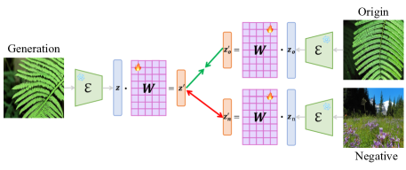
Figure 4: The implementation of learning theoretical-expected matrix $\mathbf{W}$. Specifically, in practice, we use gradient descent to optimize a metric loss function in order to learn $\mathbf{W}$.

4.3 Implementation

As illustrated in Fig. 4, we show how to learn the theoretical-expected matrix $\mathbf{W}$ in practice. Consider a triplet $\left(g,o,n\right)$, where $g$ is the generated image, $o$ is the origin used to generate $g$, and $n$ is a negative sample relative to $g$. We have:

$$\mathbf{z}=\mathcal{E}\left(g\right),\mathbf{z}_{o}=\mathcal{E}\left(o\right),\ \operatorname{and},\ \mathbf{z}_{n}=\mathcal{E}\left(n\right),$$ (8)

where $\mathcal{E}$ is the encoder of VAE. Therefore, the final loss is defined as:

$$\mathcal{L}=\mathcal{L}_{mtr}\left(\mathbf{z}\cdot\mathbf{W},\mathbf{z}_{o}\cdot\mathbf{W},\mathbf{z}_{n}\cdot\mathbf{W}\right),$$ (9)

where $\mathcal{L}_{mtr}$ is a metric learning loss function that aims to bring positive data points closer together in the embedding space while pushing negative data points further apart. We use CosFace [40] here as $\mathcal{L}_{mtr}$ for its simplicity and effectiveness. Using gradient descent, we can optimize the loss function $\mathcal{L}$ to obtain the theoretically expected matrix $\mathbf{W}$.

5 Experiments

5.1 Evaluation Protocols and Training Details

Evaluation protocols. We adopt two commonly used evaluation metrics for our ID² task: i.e., Mean Average Precision (mAP) and Top-1 Accuracy (Acc). mAP evaluates a model’s precision at various recall levels, while Acc measures the proportion of instances where the model’s top prediction exactly matches the original image. Acc is stricter as it only counts when the first guess is correct.

Training details. We distribute the optimization of the theoretically expected matrix $\mathbf{W}$ across 8 NVIDIA A100 GPUs using PyTorch [30]. The images are resized to a resolution of $256\times 256$ before being embedded by the VAE encoder. The peak learning rate is set to $3.5\times 10^{-4}$, and the Adam optimizer [16] is used.

Table 2: Publicly available models fail on the test set of OriPID.

	Method	Venue	mAP	Acc
Supervised	Swin-B [23]	ICCV	$3.9$	$2.7$
Pre-trained	ResNet-50 [12]	CVPR	$4.5$	$3.0$
Models	ConvNeXt [24]	CVPR	$4.5$	$3.1$
	EfficientNet [38]	ICML	$4.6$	$3.3$
	ViT-B [8]	ICLR	$6.2$	$4.6$
Self-	SimSiam [6]	CVPR	$1.8$	$1.0$
supervised	MoCov3 [13]	CVPR	$2.1$	$1.2$
Learning	DINOv2 [27]	TMLR	$4.3$	$2.9$
Models	MAE [14]	CVPR	$11.6$	$9.2$
	SimCLR [5]	ICML	$11.3$	$9.7$
Vision-	CLIP [34]	ICML	$2.9$	$1.8$
language	SLIP [25]	ECCV	$5.4$	$3.7$
Models	ZeroVL [7]	ECCV	$5.6$	$3.8$
	BLIP [19]	ICML	$8.3$	$5.9$
Image Copy	ASL [42]	AAAI	$5.2$	$4.1$
Detection	CNNCL [47]	PMLR	$6.3$	$5.0$
Models	BoT [41]	PMLR	$10.5$	$8.2$
	SSCD [31]	CVPR	$14.8$	$12.5$
	AnyPattern [43]	Arxiv	$29.1$	$25.7$

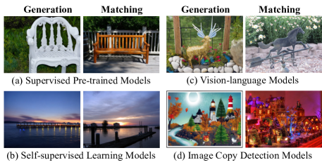
Figure 5: Examples of failure cases for each kind of model.

5.2 The Challenge from ID²

This section benchmarks popular public deep embedding models on the OriPID test dataset. As shown in Table 2 and Fig. 5, we extensively experiment on supervised pre-trained models, self-supervised learning models, vision-language models, and image copy detection models. We use these models as feature extractors, matching query features against references. The mAP and Acc are calculated by averaging the results of 7 diffusion models. Please refer to Table 8 in Supplementary for the complete results. We observe that: (1) All existing methods fail on the OriPID test dataset, highlighting the importance of constructing specialized training datasets and developing new methods. Specifically, supervised pre-trained models overly focus on category-level similarity and thus achieve a maximum mAP of $6.2\%$; self-supervised learning models handle only subtle changes and thus achieve a maximum mAP of $11.6\%$; vision-language models return matches with overall semantic consistency, achieving a maximum mAP of $8.3\%$; and image copy detection models are trained with translation patterns different from those of the ID² task, thus achieving a maximum mAP of $29.1\%$. (2) AnyPattern [43] achieves significantly higher mAP ($29.1\%$) and accuracy ($25.7\%$) compared to other methods. This is reasonable because it is designed for pattern generalization. Although the translation patterns generated by diffusion models in our ID² differ from the manually designed ones in AnyPattern, there remains some generalizability.

Table 3: VAE differs between seen and unseen diffusion models.

	Sim.	SDXL	OpDa	CoXL	Kan3	SD3	Kolor
	Conv.	$\hskip-1.13809pt0.169$	$\hskip-1.13809pt0.169$	$\hskip-1.13809pt0.169$	$\hskip-1.13809pt0.002$	-	$\hskip-1.13809pt0.169$
SD2	Embed.	$\hskip-1.13809pt0.120$	$\hskip-1.13809pt0.121$	$\hskip-1.13809pt0.120$	$\hskip-1.13809pt0.023$	-	$\hskip-1.13809pt0.120$

Table 4: Our method excels in performance while keeping efficiency. ‘mAP’ and ‘Acc’ are in percentage; ‘Train’, ‘Extract’, and ‘Match’ are in ‘h’, ‘$10^{-4}$ s/img’, and ‘$10^{-10}$ s/pair’, respectively.

			Seen $\uparrow$		Unseen $\uparrow$		Efficiency $\downarrow$
	Method	Venue	mAP	Acc	mAP	Acc	Train	Extract	Match
Similarity	Circle loss [37]	CVPR	$70.4$	$64.3$	$53.9$	$48.5$	$1.79$	$2.81$	$0.80$
-based	SoftMax [18]	NC	$82.7$	$78.3$	$55.0$	$49.4$	$2.25$	$2.81$	$0.80$
Models	CosFace [40]	CVPR	$87.1$	$83.2$	$52.2$	$46.5$	$2.43$	$2.81$	$0.80$
General-	IBN-Net [28]	ECCV	$88.6$	$85.1$	$54.6$	$49.0$	$2.03$	$3.42$	$2.14$
izable	TransMatcher [20]	NeurIPS	$65.6$	$60.3$	$65.3$	$60.7$	$1.84$	$2.30$	$941$
Models	QAConv-GS [21]	CVPR	$78.8$	$74.9$	$75.8$	$72.3$	$1.47$	$2.30$	$464$
	Embeddings of VAE	-	$51.0$	$47.0$	$46.9$	$43.0$	-	$1.59$	$4.25$
Ours	With Linear Transformation	-	$\mathbf{88.8}$	$\mathbf{86.6}$	$\mathbf{86.6}$	$\mathbf{84.5}$	$\mathbf{0.17}$	$\mathbf{1.59}$	$\mathbf{0.53}$
	Upper: Train&Test Same Domain	-	$88.8$	$86.6$	$92.0$	$90.4$	$0.17$	$1.59$	$0.53$

5.3 VAE differs between Seen and Unseen Models

A common misunderstanding is that the generalizability of our method comes from different diffusion models sharing the same or similar VAE. In Table 3, we demonstrate that the VAE encoders used in our method differ between the diffusion models for generating training and testing images: (1) The parameters of VAE encoders are different. For instance, the cosine similarity of the last convolutional layer weights of the VAE encoder between Stable Diffusion 2 and Stable Diffusion XL is only $0.169$. Furthermore, the number of channels in the last convolutional layer differs between Stable Diffusion 2 and Stable Diffusion 3. (2) The embeddings encoded by VAEs from different diffusion models vary. For instance, the average cosine similarity of VAE embeddings for 100,000 original images between Stable Diffusion 2 and Kandinsky-3 is close to $0$. Additionally, the dimension of the VAE embedding for Stable Diffusion 2 is $4,096$, whereas for Stable Diffusion 3, it is $16,384$.

5.4 The Effectiveness of our Method

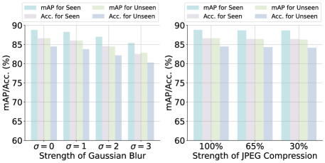
Figure 6: Our method demonstrates a certain level of robustness against different types and intensities of attacks.

This section shows the effectiveness of our method in terms of (1) generalizability, (2) efficiency, (3) robustness, and (4) the consistency between theory and experiments. The experimental results for ‘Unseen’ are obtained by averaging the results from six different unseen diffusion models.

Our method is much more generalizable than others. In Table 4, we compare our method with common similarity-based methods (incorporating domain generalization designs), all trained on the OriPID training dataset. The mAP and Acc for ‘Unseen’ are calculated by averaging the results of 6 unseen diffusion models. Please refer to Table 8 and Section 11 in Supplementary for the complete results and failure cases, respectively. We make three observations: (1) On unseen data, our method demonstrates significant performance superiority over common similarity-based models. Specifically, compared against the best one, we achieve a superiority of $+31.6\%$ mAP and $+35.1\%$ Acc. (2) Although domain generalization methods alleviate the generalization problem, they are still not satisfactory compared to ours (with at least a $-10.8\%$ mAP and $-9.1\%$ Acc). Moreover, those with the best performance suffer from severe efficiency issues, as detailed in the next section. (3) On the seen data, we achieve comparable performance with others. Specifically, there is a $0.2\%$ mAP and $1.5\%$ Acc superiority compared to the best one.

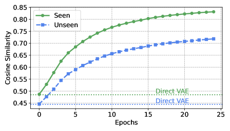
Figure 7: As expected by the theory, the cosine similarities increase w.r.t. epochs.

Table 5: Ablation for choices of VAE encoders.

	Seen $\uparrow$		Unseen $\uparrow$
VAE	mAP	Acc	mAP	Acc
Open-Sora	$86.3$	$83.5$	$86.5$	$84.2$
Open-Sora-Plan	$88.8$	$86.4$	$86.1$	$84.0$
Stable Diffusion 2	$\mathbf{88.8}$	$\mathbf{86.6}$	$\mathbf{86.6}$	$\mathbf{84.5}$

Table 6: Ablation for different supervision losses.

	Seen $\uparrow$		Unseen $\uparrow$
Supervision	mAP	Acc	mAP	Acc
SoftMax	$76.1$	$72.6$	$62.4$	$59.0$
Circle loss	$84.9$	$82.0$	$82.5$	$80.4$
CosFace	$\mathbf{88.8}$	$\mathbf{86.6}$	$\mathbf{86.6}$	$\mathbf{84.5}$

Our method outperforms others in terms of efficiency. Efficiency is crucial for the proposed task, as it often involves matching a query against a large-scale database in real-world scenarios. In Table 4, we compare the efficiency of our method with others regarding (1) training, (2) feature extraction, and (3) matching. We draw three observations: (1) Training: Learning a matrix based on VAE embeddings is more efficient compared to training deep models on raw images. Specifically, our method is $8.6$ times faster than the nearest competitor. (2) Feature extraction: Compared to other models that use deep networks, such as ViT [8], the VAE encoder we use is relatively lightweight, resulting in faster feature extraction. (3) Matching: Compared to the best domain generalization models, QAConv-GS [21], which use feature maps for matching, our method still relies on feature vectors. This leads to an $\mathbf{875}\bm{\times}$ superiority in matching speed.

Our method is relatively robust against different attacks. In the real world, the quality of an image may deteriorate during transmission. As shown in Fig. 6, we apply varying intensities of Gaussian blur and JPEG compression, following previous works such as [45, 4], to evaluate the robustness of our method. It is observed that the side effects of these attacks are relatively minor. For instance, for the unseen diffusion models, the strongest Gaussian blur ($\sigma=3$) reduces the mAP by only $3.7\%$, while the strongest compression ($30\%$) decreases the mAP by just $0.3\%$. Note that our models are not trained with these attacks.

Our training scheme successfully learns the theory-anticipated matrix $\mathbf{W}$. In the theorems, we have proven that $\mathcal{E}_{1}\left(g_{1}/g_{2}\right)\cdot\mathbf{W}=\mathcal{E}_{1}(o)\cdot\mathbf{W}$ holds ideally. In Fig. 7, we experimentally show this phenomenon. Specifically, we first calculate two cosine similarities of $<\mathcal{E}_{1}\left(g_{1}\right)\cdot\mathbf{W},\mathcal{E}_{1}(o)\cdot\mathbf{W}>$ (seen) and $<\mathcal{E}_{1}\left(g_{2}\right)\cdot\mathbf{W},\mathcal{E}_{1}(o)\cdot\mathbf{W}>$ (unseen), and then plot their changes with respect to the epochs. We observe that: (1) as expected, the two cosine similarities increase during training; and (2) the cosine similarities of the seen models are higher than those of the unseen ones, which is reasonable due to a certain degree of overfitting.

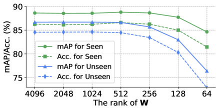
Figure 8: The change in performance w.r.t the rank of $\mathbf{W}$.

5.5 Ablation Study

In this section, we ablate the proposed method by (1) using different VAE encoders, (2) supervising the training with different loss functions, (3) exploring the minimum rank of $\mathbf{W}$, and (4) experimentally exploring beyond the theoretical guarantees.

As shown in Table 6, Table 6, Fig. 8, and Fig. 9, we observe that: (1) Our method is insensitive to the choice of VAE encoder; (2) In practice, selecting an appropriate supervision for learning $\mathbf{W}$ is essential; (3) To improve efficiency, the rank of $\mathbf{W}$ can be relatively low; and (4) Using a multilayer perceptron (MLP) with activation function instead of the theoretically expected $\mathbf{W}$ leads to overfitting. Please see the details in Supplementary (Section 12).

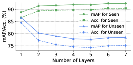
Figure 9: The change in performance w.r.t the number of layers.

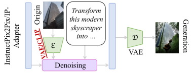
Figure 10: The image-to-image paradigm beyond our theorems.

6 Conclusion

This paper explores popular text-guided image-to-image diffusion models from a novel perspective: retrieving the original image of a query translated by these models. The proposed task, ID², is both important and timely, especially as awareness of security concerns posed by diffusion models grows. To support this task, we introduce the first ID² dataset, OriPID, designed with a focus on addressing generalization challenges. Specifically, the training set is generated by one diffusion model, while the test set is generated by seven different models. Furthermore, we propose a simple, generalizable solution with theoretical guarantees: First, we theoretically prove the existence of linear transformations that minimize the distance between the VAE embeddings of a query and its original image. Then, we demonstrate that the learned linear transformations generalize across different diffusion models, i.e., the VAE encoder and the learned transformations can effectively embed images generated by new diffusion models.

Limitation. We note that certain methods, such as InstructPix2Pix [2] and IP-Adapter [46] (see Fig. 10), perform text-guided image-to-image tasks in paradigms that go beyond the scope of our theorems. For a more detailed discussion, please refer to Supplementary (Section 13).

Supplementary Material

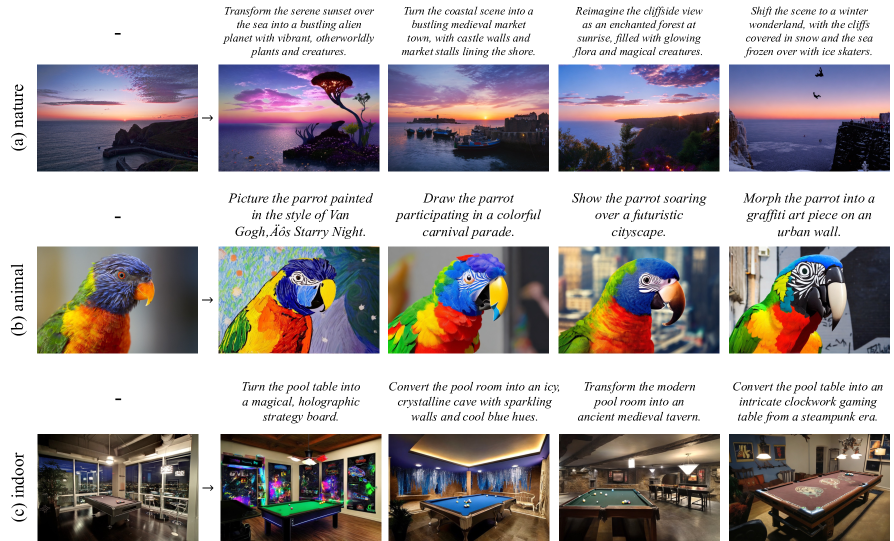
Figure 11: Illustration of prompts and corresponding generated images for 6 different subjects in our dataset. Our dataset comprehensively includes various subjects found in the real world.

7 Proofs of Lemmas

Proof.

Denote $\mathbf{z}_{0}=\mathcal{E}_{1}(o)$ and $\mathbf{z}_{0}^{\prime}$ as $\mathbf{z}_{0}$ after adding noise and denoising. Therefore, we have

$$\mathcal{E}_{1}\left(g_{1}\right)-\mathcal{E}_{1}(o)=\mathcal{E}_{1}\left(\mathcal{D}_{1}\left(\mathbf{z}_{0}^{\prime}\right)\right)-\mathbf{z}_{0}=\mathbf{z}_{0}^{\prime}-\mathbf{z}_{0},$$ (11)

where $\mathcal{D}_{1}$ is the decoder of VAE.

Given an initial data point $\mathbf{z}_{0}$, the forward process in a diffusion model adds noise to the data step by step. The expression for $\mathbf{z}_{t}$ at a specific timestep $t$ can be written as:

$$\mathbf{z}_{t}=\sqrt{\bar{\alpha_{t}}}\mathbf{z}_{0}+\sqrt{1-\bar{\alpha_{t}}}\bm{\epsilon}.$$ (12)

To denoise $\mathbf{z}_{t}$ and recover an estimate of the original data $\mathbf{z}_{0}$, the reverse process is used. A neural network $\theta$ is trained to predict the noise $\bm{\epsilon}$ added to $\mathbf{z}_{0}$. The denoised data $\mathbf{z}_{0}^{\prime}$ can be expressed as:

$$\mathbf{z}_{0}^{\prime}=\frac{1}{\sqrt{\bar{\alpha}_{t}}}\left(\mathbf{z}_{t}-\sqrt{1-\bar{\alpha}_{t}}\bm{\epsilon}_{\theta}\left(\mathbf{z}_{t},t,\mathbf{c}\right)\right).$$ (13)

Therefore, we have:

$$\begin{gathered}\mathcal{E}_{1}\left(g_{1}\right)-\mathcal{E}_{1}(o)=\mathbf{z}_{0}^{\prime}-\mathbf{z}_{0}\\ =\frac{1}{\sqrt{\bar{\alpha}_{t}}}\left(\mathbf{z}_{t}-\sqrt{1-\bar{\alpha}_{t}}\bm{\epsilon}_{\theta}\left(\mathbf{z}_{t},t,\mathbf{c}\right)\right)-\mathbf{z}_{0}\\ =\frac{1}{\sqrt{\bar{\alpha}_{t}}}\left(\sqrt{\bar{\alpha}_{t}}\mathbf{z}_{0}+\sqrt{1-\bar{\alpha}_{t}}\bm{\epsilon}-\sqrt{1-\overline{\alpha_{t}}}\bm{\epsilon}_{\theta}\left(\mathbf{z}_{t},t,\mathbf{c}\right)\right)-\mathbf{z}_{0}\\ =\frac{\sqrt{1-\bar{\alpha}_{t}}}{\sqrt{\bar{\alpha}_{t}}}\left(\bm{\epsilon}-\bm{\epsilon}_{\theta}\left(\mathbf{z}_{t},t,\mathbf{c}\right)\right).\end{gathered}$$ (14)

The Eq. 10 is proved. ∎

Proof.

Consider a matrix $\mathbf{A}\in\mathbb{R}^{m\times n}$. According to Lemma 3, there exists orthogonal matrices $\mathbf{U}\in\mathbb{R}^{m\times m}$ and $\mathbf{V}\in\mathbb{R}^{n\times n}$, and diagonal matrix $\mathbf{\Sigma}\in\mathbb{R}^{m\times n}$ with non-negative singular values, such that, $\mathbf{A}=\mathbf{U}\mathbf{\Sigma}\mathbf{V}^{*}$. Therefore, the linear equation can be transformed as:

$$\mathbf{U}\mathbf{\Sigma}\mathbf{V}^{*}\mathbf{X}=\mathbf{0}.$$ (15)

Considering $\mathbf{U}^{*}\mathbf{U}=\mathbf{I}$ and denoting $\mathbf{X}^{\prime}=\mathbf{V}^{*}\mathbf{X}$, we have $\mathbf{\Sigma}\mathbf{X}^{\prime}=\mathbf{0}$. Because $\mathbf{A}\approx\mathbf{O}$, all of its singular values approximately equals to $0$. Considering the floating-point precision we need, $\mathbf{\Sigma}\mathbf{X}^{\prime}=\mathbf{0}$ could be regarded as:

$$\left(\begin{gathered}\left(\begin{matrix}\sigma_{0}&&&\\ &\sigma_{1}&&\\ &&\ddots&\\ &&&\sigma_{r}\end{matrix}\right)\left(\begin{matrix}0&&&\\ &0&&\\ &&\ddots&\\ &&&0\end{matrix}\right)\\ \left(\begin{matrix}0&&&\\ &0&&\\ &&\ddots&\\ &&&0\end{matrix}\right)\ \left(\begin{matrix}0&&&\\ &0&&\\ &&\ddots&\\ &&&0\end{matrix}\right)\end{gathered}\right)\mathbf{X}^{\prime}=\mathbf{0},$$ (16)

where $r$ is the number of non-zero singular values. Therefore, there exists an $\mathbf{Z}^{\prime}\in\mathbb{R}^{n\times k}$ with $\text{rank}=\operatorname{min}(m,n)-r$. When $k\leqslant\operatorname{min}(m,n)-r$, $\mathbf{Z}^{\prime}$ is full rank, i.e, $\mathbf{Z}=\mathbf{V}\mathbf{Z}^{\prime}$ is an approximate full-rank solution to the linear equation $\mathbf{AX}=\mathbf{0}$. ∎

Proof.

Consider a matrix $\mathbf{A}\in\mathbb{R}^{m\times n}$. The matrix $\mathbf{A}^{*}\mathbf{A}$ is therefore symmetric and positive semi-definite, which means the matrix is diagonalizable with an eigendecomposition of the form:

$$\mathbf{A}^{*}\mathbf{A}=\mathbf{V}\Lambda\mathbf{V}^{*}=\sum_{i=1}^{n}\lambda_{i}\mathbf{v}_{i}\mathbf{v}_{i}^{*}=\sum_{i=1}^{n}\left(\sigma_{i}\right)^{2}\mathbf{v}_{i}\mathbf{v}_{i}^{*},$$ (17)

where $\mathbf{V}$ is an orthonormal matrix whose columns are the eigenvectors of $\mathbf{A}^{*}\mathbf{A}$.

We have defined the singular value $\sigma_{i}$ as the square root of the $i$-th eigenvalue; we know we can take the square root of our eigenvalues because positive semi-definite matrices can be equivalently characterized as matrices with non-negative eigenvalues.

For the $i$-th eigenvector-eigenvalue pair, we have

$$\mathbf{A}^{*}\mathbf{A}\mathbf{v}_{i}=\left(\sigma_{i}\right)^{2}\mathbf{v}_{i}.$$ (18)

Define a new vector $\mathbf{u}_{i}$, such that,

$$\mathbf{u}_{i}=\frac{\mathbf{A}\mathbf{v}_{i}}{\sigma_{i}}.$$ (19)

This construction enables $\mathbf{u}_{i}$ as a unit eigenvector of $\mathbf{A}\mathbf{A}^{*}$. Now let $\mathbf{V}$ be an $n\times n$ matrix – because $\mathbf{A}\mathbf{A}^{*}$ is $n\times n$ – where the $i$-th column is $\mathbf{v}_{i}$; let $\mathbf{U}$ be an $m\times m$ matrix – because $\mathbf{A}\mathbf{v}_{i}$ is an $m$-vector – where the $i$-th column is $\mathbf{u}_{i}$; and let $\mathbf{\Sigma}$ be a diagonal matrix whose $i$-th element is $\sigma_{i}$. Then we can express the relationships we have so far in matrix form as:

$$\mathbf{U} =\mathbf{A}\mathbf{V}\mathbf{\Sigma}^{-1},$$ (20)

$$\mathbf{U}\mathbf{\Sigma} =\mathbf{A}\mathbf{V},$$

$$\mathbf{A} =\mathbf{U}\mathbf{\Sigma}\mathbf{V}^{*},$$

where we use the fact that $\mathbf{V}\mathbf{V}^{*}=I$ and $\mathbf{\Sigma}^{-1}$ is a diagonal matrix where the $i$-th value is the reciprocal of $\sigma_{i}$. ∎

Proof.

To prove Lemma 4, we must demonstrate two directions: if a matrix $\mathbf{A}$ has a left inverse, then it must have full rank, and conversely, if a matrix $\mathbf{A}$ has full rank, then it has a left inverse.

(1) Suppose $\mathbf{A}\in\mathbb{R}^{m\times n}$ has a left inverse $\mathbf{B}\in\mathbb{R}^{n\times m}$ such that $\mathbf{B}\mathbf{A}=\mathbf{I}_{n}$. Because the $\mathbf{I}_{n}$ is of rank $n$, the matrix $\mathbf{A}\mathbf{B}$ must have rank $n$. Considering the inequality:

$$\begin{gathered}n=\text{rank}(\mathbf{BA})\leq\min(\text{rank}(\mathbf{A}),\text{rank}(\mathbf{B}))\\ \leq\text{rank}(\mathbf{A})\leq\min(m,n)\leq n\end{gathered}$$ (21)

we have $\text{rank}(\mathbf{A})=n$, i.e., $\mathbf{A}$ has full rank.

(2) Suppose $\mathbf{A}\in\mathbb{R}^{m\times n}$ has full rank, i.e., $\text{rank}(\mathbf{A})=\min(m,n)$. We have the rows of $\mathbf{A}$ are linearly independent, and thus there exists an $n\times m$ matrix $\mathbf{C}$ such that $\mathbf{C}\mathbf{A}=\mathbf{I}_{n}$. That means $\mathbf{C}$ is a left inverse of $\mathbf{A}$. ∎

8 Prompt and Generation Examples

In Fig. 11, we present several prompts with their corresponding generated images from our dataset, OriPID. The dataset comprehensively covers a wide range of subjects commonly found in real-world scenarios, such as natural sceneries, cultural architectures, lively animals, luxuriant plants, artistic paintings, and indoor items. It is important to note that in the training set, for each original image, OriPID contains 20 prompts with corresponding generated images, and for illustration, we only show 4 of them in Fig. 11.

9 Implementation of GPT-4o

As shown in Fig. 12, we request GPT-4o to generate $20$ different prompts for each original image.

+

Figure 12: The script for requesting GPT-4o to generate $20$ different prompts for each original image.

10 Complete Experiments for 7 Models

We provide two types of complete experiments for seven different diffusion models: (1) Table 8 presents the results from directly testing publicly available models on the OriPID test dataset; and (2) Table 8 shows the results from testing models that we trained on the OriPID training dataset, which contains only images generated by Stable Diffusion 2.

Table 7: The performance of publicly available models on 7 different diffusion models.

		SD2 $\uparrow$		SDXL $\uparrow$		OpDa $\uparrow$		CoXL $\uparrow$		Kan3 $\uparrow$		SD3 $\uparrow$		Kolor $\uparrow$
	Method	mAP	Acc	mAP	Acc	mAP	Acc	mAP	Acc	mAP	Acc	mAP	Acc	mAP	Acc
Supervised	Swin-B	$3.1$	$2.0$	$2.9$	$1.9$	$4.1$	$2.9$	$4.2$	$3.1$	$6.8$	$4.7$	$2.9$	$1.9$	$3.0$	$2.0$
Pre-trained	ResNet-50	$3.8$	$2.6$	$3.1$	$2.0$	$5.3$	$3.7$	$4.5$	$3.2$	$8.1$	$5.7$	$3.4$	$2.0$	$3.4$	$2.2$
Models	ConvNeXt	$3.5$	$2.1$	$3.3$	$2.2$	$4.7$	$3.3$	$5.0$	$3.5$	$8.4$	$6.2$	$3.5$	$2.4$	$3.6$	$2.6$
	EfficientNet	$2.9$	$1.9$	$2.9$	$2.0$	$4.9$	$3.4$	$5.4$	$3.9$	$8.7$	$6.5$	$3.3$	$2.2$	$4.1$	$3.0$
	ViT-B	$4.1$	$2.8$	$4.5$	$3.1$	$7.2$	$5.5$	$6.7$	$5.0$	$11.2$	$8.7$	$4.1$	$2.8$	$5.6$	$4.3$
Self-	SimSiam	$1.5$	$1.0$	$1.2$	$0.7$	$1.8$	$0.9$	$1.7$	$1.0$	$3.1$	$1.9$	$1.5$	$0.8$	$1.4$	$0.8$
supervised	MoCov3	$1.4$	$0.8$	$1.5$	$0.9$	$2.4$	$1.3$	$2.2$	$1.3$	$3.8$	$2.4$	$1.9$	$1.1$	$1.6$	$1.0$
Learning	DINOv2	$2.6$	$1.6$	$2.7$	$1.7$	$4.6$	$3.0$	$5.5$	$3.6$	$8.4$	$5.9$	$2.9$	$1.9$	$3.6$	$2.6$
Models	MAE	$14.9$	$11.4$	$10.0$	$8.0$	$13.1$	$10.5$	$8.1$	$6.4$	$17.6$	$14.3$	$11.2$	$8.5$	$6.5$	$5.1$
	SimCLR	$6.0$	$4.2$	$7.0$	$5.2$	$13.5$	$10.6$	$13.0$	$10.1$	$23.7$	$19.3$	$7.3$	$12.0$	$8.8$	$6.7$
Vision-	CLIP	$2.6$	$1.7$	$2.1$	$1.4$	$3.1$	$2.1$	$3.2$	$2.0$	$4.2$	$2.7$	$2.5$	$1.6$	$2.1$	$0.7$
language	SLIP	$5.6$	$3.8$	$3.5$	$2.3$	$5.8$	$4.0$	$4.9$	$3.3$	$9.1$	$6.7$	$5.4$	$3.5$	$3.8$	$2.5$
Models	ZeroVL	$5.2$	$3.5$	$4.4$	$2.9$	$6.4$	$4.4$	$4.5$	$3.2$	$9.8$	$6.9$	$4.7$	$3.0$	$4.3$	$3.0$
	BLIP	$6.8$	$4.8$	$6.5$	$4.5$	$9.9$	$7.0$	$8.7$	$6.3$	$13.8$	$10.2$	$6.0$	$3.9$	$6.4$	$4.5$
Image Copy	ASL	$2.3$	$1.7$	$3.0$	$2.3$	$5.6$	$4.4$	$5.7$	$4.6$	$10.3$	$8.7$	$2.7$	$2.1$	$3.7$	$2.9$
Detection	CNNCL	$4.0$	$2.9$	$4.2$	$3.2$	$8.3$	$6.7$	$5.7$	$4.5$	$12.2$	$9.9$	$3.7$	$2.7$	$6.3$	$5.0$
Models	BoT	$6.6$	$4.9$	$6.1$	$4.4$	$10.4$	$8.2$	$12.5$	$10.2$	$20.6$	$16.8$	$7.4$	$5.4$	$9.3$	$7.3$
	SSCD	$9.7$	$7.7$	$8.7$	$6.8$	$16.4$	$14.0$	$18.1$	$15.6$	$28.1$	$24.6$	$9.0$	$6.8$	$14.1$	$11.9$
	AnyPattern	$17.6$	$14.3$	$18.5$	$15.7$	$33.0$	$29.2$	$37.8$	$34.0$	$48.0$	$43.9$	$18.2$	$15.0$	$30.7$	$27.5$

Table 8: The performance of our trained models on 7 different diffusion models. Note that these models are trained on images generated by SD2 and tested on images from multiple models.

		SD2 $\uparrow$		SDXL $\uparrow$		OpDa $\uparrow$		CoXL $\uparrow$		Kan3 $\uparrow$		SD3 $\uparrow$		Kolor $\uparrow$
	Method	mAP	Acc	mAP	Acc	mAP	Acc	mAP	Acc	mAP	Acc	mAP	Acc	mAP	Acc
Similarity-	Circle loss	$70.4$	$64.3$	$56.2$	$50.1$	$56.5$	$51.8$	$41.6$	$37.0$	$60.0$	$53.8$	$65.6$	$59.3$	$43.5$	$39.2$
based	SoftMax	$82.7$	$78.3$	$62.4$	$56.5$	$58.3$	$53.0$	$37.3$	$32.2$	$52.5$	$46.0$	$75.9$	$70.2$	$43.6$	$38.7$
Models	CosFace	$87.1$	$83.2$	$63.7$	$58.2$	$56.7$	$51.7$	$30.5$	$25.2$	$47.5$	$40.6$	$71.5$	$65.5$	$43.0$	$38.0$
General-	IBN-Net	$88.6$	$85.1$	$65.7$	$60.1$	$59.4$	$54.2$	$33.3$	$28.3$	$49.8$	$42.8$	$74.0$	$68.3$	$45.4$	$40.5$
izable	TransMatcher	$65.6$	$60.3$	$60.6$	$55.8$	$67.9$	$63.6$	$61.7$	$57.4$	$68.9$	$64.2$	$64.7$	$59.2$	$67.9$	$63.9$
Models	QAConv-GS	$78.8$	$74.9$	$71.6$	$67.5$	$77.4$	$74.3$	$73.6$	$70.5$	$75.2$	$71.2$	$77.3$	$73.6$	$79.5$	$76.9$
	VAE Embed.	$51.0$	$47.0$	$38.3$	$33.8$	$42.3$	$38.6$	$51.6$	$48.8$	$54.7$	$50.4$	$47.7$	$42.9$	$46.9$	$43.6$
Ours	Linear Trans.	$\hskip-1.13809pt\mathbf{88.8}$	$\hskip-1.13809pt\mathbf{86.6}$	$\hskip-1.13809pt\mathbf{81.5}$	$\hskip-1.13809pt\mathbf{78.8}$	$\hskip-1.13809pt\mathbf{87.3}$	$\hskip-1.13809pt\mathbf{85.3}$	$\hskip-1.13809pt\mathbf{89.3}$	$\hskip-1.13809pt\mathbf{87.7}$	$\hskip-1.13809pt\mathbf{85.7}$	$\hskip-1.13809pt\mathbf{83.3}$	$\hskip-1.13809pt\mathbf{85.7}$	$\hskip-1.13809pt\mathbf{82.9}$	$\hskip-1.13809pt\mathbf{90.3}$	$\hskip-1.13809pt\mathbf{88.8}$
	Upper	$88.8$	$86.6$	$84.9$	$82.4$	$90.8$	$89.2$	$93.1$	$91.9$	$95.4$	$94.3$	$93.7$	$92.0$	$94.0$	$92.8$

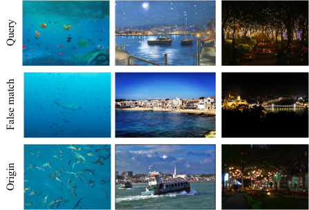
Figure 13: This illustration shows failure cases predicted by our method. We have identified that our model may fail when encountering hard negative samples.

11 Failure Cases and Potential Directions

Failure cases. As shown in Fig. 13, we observe that our model may fail when negative samples are too visually similar to the queries. This hard negative problem is reasonable because our method relies on the VAE embeddings, which capture high-level representations and is insensitive to subtle changes. As a result, visually similar negative samples can produce embeddings that are close to those of the queries, leading to inaccurate matchings.

Potential directions. The hard negative problem has been studied in the Image Copy Detection (ICD) community, as exemplified by ASL [42]. It learns to assign a larger norm to the deep features of images that contain more content or information. However, this method cannot be directly used in our scenario because the query and reference here do not have a simple relationship in terms of information amount. Nevertheless, it offers a promising research direction from the perspective of information. Specifically, on one hand, the noise-adding and denoising processes result in a loss of information, while on the other hand, the guided text introduces new information into the output.

12 Details of Ablation Studies

Our method is insensitive to the choice of VAE encoder. In Table 6, we replace the VAE encoder from Stable Diffusion 2 with two different encoders from Open-Sora [48] and Open-Sora-Plan [32]. It is observed that, despite using significantly different well-trained VAEs, such as ones for videos, the performance drop is minimal (less than $1\%$). This observation experimentally extends the Eq. 1 from $\mathcal{E}_{1}\left(g_{1}\right)\cdot\mathbf{W}=\mathcal{E}_{1}(o)\cdot\mathbf{W}$ to $\mathcal{E}_{2}\left(g_{1}\right)\cdot\mathbf{W}=\mathcal{E}_{2}(o)\cdot\mathbf{W}$, where $\mathcal{E}_{2}$ is an encoder from a totally different VAE.

In practice, selecting an appropriate supervision for learning $\mathbf{W}$ is essential. In Table 6, we replace the used supervision CosFace [40] with two weaker supervisions, i.e., SoftMax [18] and Circle loss [37]. We observe that switching to Circle loss results in a drop in mAP for seen and unseen categories by $3.9\%$ and $4.1\%$, respectively. Furthermore, using SoftMax leads to mAP drops of $12.7\%$ and $24.2\%$ for the two categories, respectively. We infer this is because: while our theorems guarantee the distance between a translation and its origin, many negative samples serve as distractors during retrieval. Without appropriate hard negative solutions, these distractors compromise the final performance.

To improve efficiency, the rank of $\mathbf{W}$ can be relatively low. Assume the matrix $\mathbf{W}$ has a shape of $n\times m$, where $n$ is the dimension of the VAE embedding and $m$ is a hyperparameter. We show that $\mathbf{W}$ is approximately full-rank in the proof of existence, and expect that $m\leq n$ in the proof of generalization. Therefore, the rank of $\mathbf{W}$ is $m$. Experimentally, $n=4,096$, and we explore the minimum rank of $\mathbf{W}$ from $4,096$ as shown in Fig. 8. It is observed that: (1) From $4,096$ to $512$, the performance remains nearly unchanged. This suggests that we can train a relatively low-rank $\mathbf{W}$ to improve efficiency in real-world applications. (2) It is expected to see a performance decrease when reducing the rank from $512$ to $64$. This is because a matrix with too low rank cannot carry enough information to effectively linearly transform the VAE embeddings.

Using a multilayer perceptron (MLP) with activation function instead of the theoretically expected $\mathbf{W}$ leads to overfitting. In the theoretical section, we proved the existence and generalization of $\mathbf{W}$ using concepts from diffusion models and linear algebra. A natural experimental extension of this is to use an MLP with activation functions to replace the simple linear transformation ($\mathbf{W}$). Although linear algebra theory cannot guarantee these cases, we can still explore them experimentally. Experimentally, we increase the number of layers from $1$ to $7$, all using ReLU activation and residual connections. As shown in Fig. 9, we observe overfitting in one type of diffusion model. Specifically, on one hand, the performance on seen diffusion models improves. For example, with 2 layers, the mAP increases to $91.4\%$ ($+2.6\%$), and Acc rises to $89.4\%$ ($+2.8\%$). However, on the other hand, a significant performance drop is observed on unseen diffusion models: with 2 layers, the mAP decreases from $86.6\%$ to $80.3\%$ ($-6.3\%$), and Acc drops from $84.5\%$ to $77.3\%$ ($-7.2\%$). The performance drop becomes even more severe when using more layers.

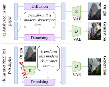
Figure 14: Different paradigms used by text-guided image-to-image translations.

13 Limitations and Future Works

Limitations. Although the paradigm analyzed in the main paper (Fig. 14 (a)) is the simplest approach for text-guided image-to-image translation and serves as the default mode in the $\mathtt{AutoPipelineForImage2Image}$ of $\mathtt{diffusers}$, we also observe the existence of an alternative paradigm, as shown in Fig. 14 (b). While this paradigm lies beyond our theoretical guarantees, we can still analyze it experimentally, as demonstrated in Table 9. Interestingly, we find that (1) our method generalizes well to InstructP2P, which still uses a VAE encoder to embed the original images; and (2) all methods, including ours, fail on IP-Adapter, which uses CLIP for encoding. We also try the linear transformed CLIP embedding, but it still fails to generalize ($36.6\%$ mAP and $27.8\%$ Acc). Based on these experiments, we conclude with a hypothesis about the upper limit of our method:

Future Works. Future works may focus on (1) providing a theoretical proof for Hypothesis 1, and (2) developing new generalization methods for text-guided image-to-image based on CLIP encodings.

Table 9: The generalization results on InstructPix2Pix [2] and IP-Adapter [46]. No method succeeds in generalizing to IP-Adapter.

		InstructP2P $\uparrow$		IP-Adapter $\uparrow$
	Method	mAP	Acc	mAP	Acc
Similarity	Circle loss	$44.9$	$42.7$	$6.2$	$4.0$
-based	SoftMax	$21.5$	$19.2$	$5.8$	$3.5$
Models	CosFace	$20.1$	$17.7$	$1.5$	$0.9$
General-	IBN-Net	$21.4$	$18.9$	$1.5$	$0.8$
izable	TransMatcher	$56.6$	$54.5$	$2.7$	$1.4$
Models	QAConv-GS	$55.1$	$53.0$	$1.2$	$0.6$
	VAE Embed.	$68.2$	$67.1$	$0.2$	$0.1$
Ours	Linear Trans. VAE	$80.7$	$79.2$	$0.4$	$0.2$

References

- Arkhipkin et al. [2023] Vladimir Arkhipkin, Andrei Filatov, Viacheslav Vasilev, Anastasia Maltseva, Said Azizov, Igor Pavlov, Julia Agafonova, Andrey Kuznetsov, and Denis Dimitrov. Kandinsky 3.0 technical report. arXiv preprint arXiv:2312.03511, 2023.
- Brooks et al. [2023] Tim Brooks, Aleksander Holynski, and Alexei A Efros. Instructpix2pix: Learning to follow image editing instructions. In Proceedings of the IEEE/CVF Conference on Computer Vision and Pattern Recognition, pages 18392–18402, 2023.
- Chen et al. [2023] Chuan Chen, Zhenpeng Wu, Yanyi Lai, Wenlin Ou, Tianchi Liao, and Zibin Zheng. Challenges and remedies to privacy and security in aigc: Exploring the potential of privacy computing, blockchain, and beyond. arXiv preprint arXiv:2306.00419, 2023.
- Chen et al. [2024] Jiaxuan Chen, Jieteng Yao, and Li Niu. A single simple patch is all you need for ai-generated image detection. arXiv preprint arXiv:2402.01123, 2024.
- Chen et al. [2020] Ting Chen, Simon Kornblith, Mohammad Norouzi, and Geoffrey Hinton. A simple framework for contrastive learning of visual representations. In International conference on machine learning, pages 1597–1607. PMLR, 2020.
- Chen and He [2021] Xinlei Chen and Kaiming He. Exploring simple siamese representation learning. In Proceedings of the IEEE/CVF conference on computer vision and pattern recognition, pages 15750–15758, 2021.
- Cui et al. [2022] Quan Cui, Boyan Zhou, Yu Guo, Weidong Yin, Hao Wu, Osamu Yoshie, and Yubo Chen. Contrastive vision-language pre-training with limited resources. In European Conference on Computer Vision, pages 236–253. Springer, 2022.
- Dosovitskiy et al. [2021] Alexey Dosovitskiy, Lucas Beyer, Alexander Kolesnikov, Dirk Weissenborn, Xiaohua Zhai, Thomas Unterthiner, Mostafa Dehghani, Matthias Minderer, Georg Heigold, Sylvain Gelly, Jakob Uszkoreit, and Neil Houlsby. An image is worth 16x16 words: Transformers for image recognition at scale. ICLR, 2021.
- Esser et al. [2024] Patrick Esser, Sumith Kulal, Andreas Blattmann, Rahim Entezari, Jonas Müller, Harry Saini, Yam Levi, Dominik Lorenz, Axel Sauer, Frederic Boesel, et al. Scaling rectified flow transformers for high-resolution image synthesis. In Forty-first International Conference on Machine Learning, 2024.
- Fan et al. [2023] Mingyuan Fan, Cen Chen, Chengyu Wang, and Jun Huang. On the trustworthiness landscape of state-of-the-art generative models: A comprehensive survey. arXiv preprint arXiv:2307.16680, 2023.
- Fernandez et al. [2023] Pierre Fernandez, Matthijs Douze, Hervé Jégou, and Teddy Furon. Active image indexing. In International Conference on Learning Representations (ICLR), 2023.
- He et al. [2016] Kaiming He, Xiangyu Zhang, Shaoqing Ren, and Jian Sun. Deep residual learning for image recognition. In Proceedings of the IEEE conference on computer vision and pattern recognition, pages 770–778, 2016.
- He et al. [2020] Kaiming He, Haoqi Fan, Yuxin Wu, Saining Xie, and Ross Girshick. Momentum contrast for unsupervised visual representation learning. In Proceedings of the IEEE/CVF conference on computer vision and pattern recognition, pages 9729–9738, 2020.
- He et al. [2022] Kaiming He, Xinlei Chen, Saining Xie, Yanghao Li, Piotr Dollár, and Ross Girshick. Masked autoencoders are scalable vision learners. In Proceedings of the IEEE/CVF conference on computer vision and pattern recognition, pages 16000–16009, 2022.
- Izquierdo [2023] Alexander Izquierdo. Opendallev1.1, 2023.
- Kingma [2014] Diederik P Kingma. Adam: A method for stochastic optimization. arXiv preprint arXiv:1412.6980, 2014.
- KolorsTeam [2024] KolorsTeam. Kolors: Effective training of diffusion model for photorealistic text-to-image synthesis. 2024.
- LeCun et al. [1989] Yann LeCun, Bernhard Boser, John S Denker, Donnie Henderson, Richard E Howard, Wayne Hubbard, and Lawrence D Jackel. Backpropagation applied to handwritten zip code recognition. Neural computation, 1(4):541–551, 1989.
- Li et al. [2022] Junnan Li, Dongxu Li, Caiming Xiong, and Steven Hoi. Blip: Bootstrapping language-image pre-training for unified vision-language understanding and generation. In International Conference on Machine Learning, pages 12888–12900. PMLR, 2022.
- Liao and Shao [2021] Shengcai Liao and Ling Shao. Transmatcher: Deep image matching through transformers for generalizable person re-identification. Advances in Neural Information Processing Systems, 34:1992–2003, 2021.
- Liao and Shao [2022] Shengcai Liao and Ling Shao. Graph sampling based deep metric learning for generalizable person re-identification. In Proceedings of the IEEE/CVF Conference on Computer Vision and Pattern Recognition, pages 7359–7368, 2022.
- Lin et al. [2024] Li Lin, Neeraj Gupta, Yue Zhang, Hainan Ren, Chun-Hao Liu, Feng Ding, Xin Wang, Xin Li, Luisa Verdoliva, and Shu Hu. Detecting multimedia generated by large ai models: A survey. arXiv preprint arXiv:2402.00045, 2024.
- Liu et al. [2021] Ze Liu, Yutong Lin, Yue Cao, Han Hu, Yixuan Wei, Zheng Zhang, Stephen Lin, and Baining Guo. Swin transformer: Hierarchical vision transformer using shifted windows. In Proceedings of the IEEE/CVF international conference on computer vision, pages 10012–10022, 2021.
- Liu et al. [2022] Zhuang Liu, Hanzi Mao, Chao-Yuan Wu, Christoph Feichtenhofer, Trevor Darrell, and Saining Xie. A convnet for the 2020s. In Proceedings of the IEEE/CVF conference on computer vision and pattern recognition, pages 11976–11986, 2022.
- Mu et al. [2022] Norman Mu, Alexander Kirillov, David Wagner, and Saining Xie. Slip: Self-supervision meets language-image pre-training. In European Conference on Computer Vision, pages 529–544. Springer, 2022.
- OpenAI [2024] OpenAI. Hello gpt-4o, 2024.
- Oquab et al. [2023] Maxime Oquab, Timothée Darcet, Theo Moutakanni, Huy V. Vo, Marc Szafraniec, Vasil Khalidov, Pierre Fernandez, Daniel Haziza, Francisco Massa, Alaaeldin El-Nouby, Russell Howes, Po-Yao Huang, Hu Xu, Vasu Sharma, Shang-Wen Li, Wojciech Galuba, Mike Rabbat, Mido Assran, Nicolas Ballas, Gabriel Synnaeve, Ishan Misra, Herve Jegou, Julien Mairal, Patrick Labatut, Armand Joulin, and Piotr Bojanowski. Dinov2: Learning robust visual features without supervision, 2023.
- Pan et al. [2018] Xingang Pan, Ping Luo, Jianping Shi, and Xiaoou Tang. Two at once: Enhancing learning and generalization capacities via ibn-net. In Proceedings of the european conference on computer vision (ECCV), pages 464–479, 2018.
- Papakipos et al. [2022] Zoë Papakipos, Giorgos Tolias, Tomas Jenicek, Ed Pizzi, Shuhei Yokoo, Wenhao Wang, Yifan Sun, Weipu Zhang, Yi Yang, Sanjay Addicam, et al. Results and findings of the 2021 image similarity challenge. In NeurIPS 2021 Competitions and Demonstrations Track, pages 1–12. PMLR, 2022.
- Paszke et al. [2019] Adam Paszke, Sam Gross, Francisco Massa, Adam Lerer, James Bradbury, Gregory Chanan, Trevor Killeen, Zeming Lin, Natalia Gimelshein, Luca Antiga, et al. Pytorch: An imperative style, high-performance deep learning library. Advances in neural information processing systems, 32, 2019.
- Pizzi et al. [2022] Ed Pizzi, Sreya Dutta Roy, Sugosh Nagavara Ravindra, Priya Goyal, and Matthijs Douze. A self-supervised descriptor for image copy detection. In Proceedings of the IEEE/CVF Conference on Computer Vision and Pattern Recognition, pages 14532–14542, 2022.
- PKU-Yuan and etc. [2024] Lab PKU-Yuan and Tuzhan AI etc. Open-sora-plan, 2024.
- Podell et al. [2024] Dustin Podell, Zion English, Kyle Lacey, Andreas Blattmann, Tim Dockhorn, Jonas Müller, Joe Penna, and Robin Rombach. SDXL: Improving latent diffusion models for high-resolution image synthesis. In The Twelfth International Conference on Learning Representations, 2024.
- Radford et al. [2021] Alec Radford, Jong Wook Kim, Chris Hallacy, Aditya Ramesh, Gabriel Goh, Sandhini Agarwal, Girish Sastry, Amanda Askell, Pamela Mishkin, Jack Clark, et al. Learning transferable visual models from natural language supervision. In International conference on machine learning, pages 8748–8763. PMLR, 2021.
- Recoilme [2023] Recoilme. Colorfulxl-lightning, 2023.
- Rombach et al. [2022] Robin Rombach, Andreas Blattmann, Dominik Lorenz, Patrick Esser, and Björn Ommer. High-resolution image synthesis with latent diffusion models. In Proceedings of the IEEE/CVF Conference on Computer Vision and Pattern Recognition (CVPR), pages 10684–10695, 2022.
- Sun et al. [2020] Yifan Sun, Changmao Cheng, Yuhan Zhang, Chi Zhang, Liang Zheng, Zhongdao Wang, and Yichen Wei. Circle loss: A unified perspective of pair similarity optimization. In Proceedings of the IEEE/CVF conference on computer vision and pattern recognition, pages 6398–6407, 2020.
- Tan and Le [2019] Mingxing Tan and Quoc Le. Efficientnet: Rethinking model scaling for convolutional neural networks. In International conference on machine learning, pages 6105–6114. PMLR, 2019.
- Thomee et al. [2016] Bart Thomee, David A Shamma, Gerald Friedland, Benjamin Elizalde, Karl Ni, Douglas Poland, Damian Borth, and Li-Jia Li. Yfcc100m: The new data in multimedia research. Communications of the ACM, 59(2):64–73, 2016.
- Wang et al. [2018] Hao Wang, Yitong Wang, Zheng Zhou, Xing Ji, Dihong Gong, Jingchao Zhou, Zhifeng Li, and Wei Liu. Cosface: Large margin cosine loss for deep face recognition. In Proceedings of the IEEE conference on computer vision and pattern recognition, pages 5265–5274, 2018.
- Wang et al. [2021] Wenhao Wang, Weipu Zhang, Yifan Sun, and Yi Yang. Bag of tricks and a strong baseline for image copy detection. arXiv preprint arXiv:2111.08004, 2021.
- Wang et al. [2023a] Wenhao Wang, Yifan Sun, and Yi Yang. A benchmark and asymmetrical-similarity learning for practical image copy detection. In Proceedings of the AAAI Conference on Artificial Intelligence, pages 2672–2679, 2023a.
- Wang et al. [2024a] Wenhao Wang, Yifan Sun, Zhentao Tan, and Yi Yang. Anypattern: Towards in-context image copy detection. In arXiv preprint arXiv:2404.13788, 2024a.
- Wang et al. [2024b] Wenhao Wang, Yifan Sun, and Yi Yang. Pattern-expandable image copy detection. International Journal of Computer Vision, pages 1–17, 2024b.
- Wang et al. [2023b] Zhendong Wang, Jianmin Bao, Wengang Zhou, Weilun Wang, Hezhen Hu, Hong Chen, and Houqiang Li. Dire for diffusion-generated image detection. In Proceedings of the IEEE/CVF International Conference on Computer Vision, pages 22445–22455, 2023b.
- Ye et al. [2023] Hu Ye, Jun Zhang, Sibo Liu, Xiao Han, and Wei Yang. Ip-adapter: Text compatible image prompt adapter for text-to-image diffusion models. 2023.
- Yokoo [2021] Shuhei Yokoo. Contrastive learning with large memory bank and negative embedding subtraction for accurate copy detection. arXiv preprint arXiv:2112.04323, 2021.
- Zheng et al. [2024] Zangwei Zheng, Xiangyu Peng, Tianji Yang, Chenhui Shen, Shenggui Li, Hongxin Liu, Yukun Zhou, Tianyi Li, and Yang You. Open-sora: Democratizing efficient video production for all, 2024.