${\mathcal{K}}$-Lorentzian and ${\mathcal{K}}$-CLC Polynomials in Stability Analysis

Abstract.

We study the class of ${\mathcal{K}}$-Lorentzian polynomials, a generalization of the distinguished class of Lorentzian polynomials. As shown in [BD24], the set of ${\mathcal{K}}$-Lorentzian polynomials is equivalent to the set of ${\mathcal{K}}$-completely log-concave (aka ${\mathcal{K}}$-CLC) forms. Throughout this paper, we interchangeably use the terms ${\mathcal{K}}$-Lorentzian polynomials for the homogeneous setting and ${\mathcal{K}}$-CLC polynomials for the non-homogeneous setting. By introducing an alternative definition of ${\mathcal{K}}$-CLC polynomials through univariate restrictions, we establish that any strictly ${\mathcal{K}}$-CLC polynomial of degree $d\leq 4$ is Hurwitz-stable polynomial over ${\mathcal{K}}$. Additionally, we characterize the conditions under which a strictly ${\mathcal{K}}$-CLC of degree $d\geq 5$ is Hurwitz-stable over ${\mathcal{K}}$. Furthermore, we associate the largest possible proper cone, denoted by ${\mathcal{K}}(f,v)$, with a given ${\mathcal{K}}$-Lorentzian polynomial $f$ in the direction $v\in\operatorname{int}{\mathcal{K}}$. Finally, we investigate applications of ${\mathcal{K}}$-CLC polynomials in the stability analysis of evolution variational inequalities (EVI) dynamical systems governed by differential equations and inequality constraints.

1. Introduction

${\mathcal{K}}$-Lorentzian polynomials are introduced and studied by Brändén and Leake in [BL23a], and by Blekherman and Dey in [BD24]. Our approach in [BD24] not only generalizes Lorentzian polynomials introduced by June Huh and Petter Brändén in [BH20] and simultaneously by Anari, Oveis Gharan and Vinzant [AGV21] (under the name of completely log-concave polynomials), but also provides a unified framework for extending this class. In [BD24], we established a link between ${\mathcal{K}}$-Lorentzian polynomials and ${\mathcal{K}}$-nonnegative matrices, which arise in the context of the generalized Perron-Frobenius Theorem. Leveraging this connection, we presented a further characterization of ${\mathcal{K}}$-Lorentzian polynomials over self-dual cones, yielding an additional necessary and sufficient condition for Lorentzian polynomials over the nonnegative orthant.

We observe that for any ${\mathcal{K}}$-Lorentzian polynomial over self-dual cone ${\mathcal{K}}$, the nonsingular Hessian matrices evaluated at points $a\in{\mathcal{K}}$ satisfy the generalized Perron-Frobenius Theorem. We introduce an alternative definition of ${\mathcal{K}}$-CLC polynomials by restricting them to lines, which enables the analysis of log-concavity in the coefficients of the resulting univariate polynomials. Furthermore, leveraging the structure of the coefficients, we show that any strictly ${\mathcal{K}}$-CLC polynomial of degree $d\leq 4$ is Hurwitz-stable over ${\mathcal{K}}$, [see Theorem˜4.20]. Moreover, for degree $d\geq 5$, we characterize the class of strictly ${\mathcal{K}}$-CLC polynomials which are Hurwitz-stable over ${\mathcal{K}}$ using a known result to characterize Hurwitz-stability for univariate polynomials of degree $d\geq 5$, [see Theorem˜4.21]. An example of a strictly CLC polynomial of $d=5$ that is not Hurwitz stable is provided. This plays a crucial role in stability analysis of a dynamical system when trajectories are constrained on certain regions.

Throughout this article, unless otherwise stated, we assume that ${\mathcal{K}}$ is a proper convex cone. A natural progression is to determine an appropriate ${\mathcal{K}}$ for a given ${\mathcal{K}}$-Lorentzian polynomial, similar to the way hyperbolicity cones correspond to hyperbolic polynomials. To achieve this, we identify the largest possible proper cone w.r.t a direction $v$, denoted by ${\mathcal{K}}(f,v)$, associated with a ${\mathcal{K}}$-Lorentzian candidate. We provide a characterization of the interior of the closed cone ${\mathcal{K}}(f,v)$, [see Theorem˜5.5] and demonstrate that if $f$ is ${\mathcal{K}}$-Lorentzian on ${\mathcal{K}}(f,v)$, then ${\mathcal{K}}(f,v)$ is a convex set, [see Theorem˜5.7]. Notably, when $f$ is a hyperbolic polynomial, ${\mathcal{K}}(f,v)$ corresponds to the hyperbolicity cone of $f$ in the direction $v$. The Rayleigh -Difference polynomial, defined as $\Delta_{i,j}f(x):=\partial_{i}f\partial_{j}f-f\partial_{i}\partial_{j}f$, plays a significant role in optimization and sampling algorithms (fast algorithm in MCMC methods), especially in high-dimensional, non-convex settings. In statistics, many distributions (e.g., Gaussian, exponential) are log-concave. The nonnegative condition of the Rayleigh difference polynomial ensures the preservation of log-concavity under marginalization or convolution. We demonstrate that for a ${\mathcal{K}}$-Lorentzian polynomial $f$, the Rayleigh difference polynomials $D_{w}f.D_{v}f-f\cdot D_{w}D_{v}f$ are nonnegative over ${\mathcal{K}}$ for all $v,w\in{\mathcal{K}}$, [see Theorem˜5.14]. An additional area of exploration involves the semipositive cone, obtained as the intersection of a hyperbolicity cone with the nonnegative orthant, for a hyperbolic generating polynomial $f_{A}$ associated with a nonsingular semipositive matrix $A$, [see Proposition˜5.15]. This class of polynomials facilitates the characterization of the intersection cone, as the ${\mathcal{K}}$-semipositive cone, [see Theorem˜5.21].

The Hurwitz-stability of strictly CLC polynomial $f(t)$ over the interval $t\geq 0$ establishes a connection to stable LTI dynamical systems of the form $\frac{dx}{dt}=Ax$, where the characteristic polynomial $\chi(A)=f(t)$, [see Theorem˜6.2] and Theorem˜6.4]. Moreover, we introduce a method to assess the (Lyapunov-type) stability w.r.t ${\mathcal{K}}$ of certain dynamical systems through ${\mathcal{K}}$-Lorentzian polynomials. This class is known as the Evolution Variational Inequality (EVI), and characterized by a combination of differential equations and inequality constraints. These systems describe the evolution of a state $x(t)$ in time, constrained by a variational inequality associated with a convex set and a functional that defines the system dynamics. Specifically, for EVI systems, we show that even if the system lacks global (asymptotic) stability, it can still exhibit (asymptotic) stability w.r.t ${\mathcal{K}}$ via ${\mathcal{K}}$-CLC polynomials, [see Theorem˜6.18 and Theorem˜6.23]. Additionally, ${\mathcal{K}}$-Lorentzian polynomials can be employed to identify regions where stability is achievable. EVIs often arise as the continuous-time counterpart of optimization problems constrained by convex sets. For example, they can model gradient flows constrained by feasibility conditions, where the goal is to minimize a convex function $f(x)$ subject to $x\in{\mathcal{K}}$. EVIs are extensively used in applied mathematics and various scientific disciplines, with applications spanning control theory (e.g., when state variables or control inputs are constrained), game theory (such as saddle-point dynamics and Nash equilibrium computation), machine learning (e.g., gradient descent flows with constraints), and traffic and network flow analysis. For additional applications, see [GB04] and the references therein.

The rest of the paper is structured as follows: In Section˜2 we recall the definitions and essential theorems that will be utilized in the following sections. In Section˜3, we develop several key properties of ${\mathcal{K}}$-Lorentzian polynomials. Notably, we introduce an alternative definition of ${\mathcal{K}}$-CLC polynomials (which need not be forms) by restricting them to specific lines, allowing us to derive important necessary conditions for ${\mathcal{K}}$-CLC polynomials. One such condition highlights the log-concavity properties of the coefficients of the univariate restricted polynomials. Section˜4 explores the connection between Hurwitz-stability over ${\mathcal{K}}$ and strictly ${\mathcal{K}}$-CLC polynomials, noting that not all strictly ${\mathcal{K}}$-CLC polynomials of degree $d\geq 5$ are Hurwitz-stable, and examining cases where they are. In Section˜5, the largest proper cone ${\mathcal{K}}(f,v)$ with a given ${\mathcal{K}}$-CLC polynomial $f$ is introduced, along with nonnegativity results for Rayleigh difference polynomials and discussions on ${\mathcal{K}}$-semipositive cones. Finally, Section˜6 demonstrates how stability analysis of EVI systems is achieved through ${\mathcal{K}}$-CLC polynomials.

2. State of the Art

A nonempty convex set ${\mathcal{K}}\subseteq{\mathbb{R}}^{n}$ is said to be a cone if $c{\mathcal{K}}\subseteq{\mathcal{K}}$ for all $c\geq 0$. A cone ${\mathcal{K}}$ is called proper if it is closed (in the Euclidean topology on ${\mathbb{R}}^{n}$), pointed (i.e., ${\mathcal{K}}\cap(-{\mathcal{K}})=\{0\}$), and solid (i.e., the topological interior of ${\mathcal{K}}$, denoted as $\operatorname{int}{\mathcal{K}}$, is nonempty).

Let ${\mathbb{R}}[x]$ represent the space of $n$-variate polynomials over ${\mathbb{R}}$, and ${\mathbb{R}}[x]_{\leq d}$ represent the space of $n$-variate polynomials over ${\mathbb{R}}$ with degree at most $d$ and ${\mathbb{R}}[x]^{d}_{n}$ denote the space of real homogeneous polynomials (aka forms) in $n$ variables of degree $d$. A polynomial $f\in{\mathbb{R}}[x]$ is said to be (strictly) log-concave at a point $a\in{\mathbb{R}}^{n}$ if $f(a)>0$, and $\log f$ is a (strictly) concave function at $a$, i.e. the Hessian of $\log f$ is negative semidefinite (negative definite) at $a$. A polynomial $f\in{\mathbb{R}}[x]$ is log-concave on a proper cone ${\mathcal{K}}\subset{\mathbb{R}}^{n}$ if $f$ is log-concave at every point of the interior of ${\mathcal{K}}$. By convention, the zero polynomial is log-concave (but not strictly log-concave) at all points of ${\mathbb{R}}^{n}$.

If ${\mathcal{K}}={\mathcal{K}}^{\ast}$, a self-dual cone, then $K$ is closed, pointed, and full dimensional[BF76]. We denote quadratic forms by a lower case letter, and the matrix of the quadratic form by the corresponding upper case letter, i.e. if $q$ is a quadratic form, then its matrix is $Q$ and $q(x)=x^{t}Qx$.

For a point $a\in{\mathbb{R}}^{n}$ and $f\in{\mathbb{R}}[x]$, $D_{a}f$ denotes the directional derivative of $f$ in direction $a$: $D_{a}f=\sum_{i=1}^{n}a_{i}\frac{\partial f}{\partial x_{i}}$. Here are the definitions of the ${\mathcal{K}}$-completely log-concave polynomials and ${\mathcal{K}}$-Lorentzian forms.

Definition 2.1.

[BD24] A polynomial (form) $f\in{\mathbb{R}}[x]_{\leq d}$ is called a ${\mathcal{K}}$-completely log-concave aka ${\mathcal{K}}$-CLC (form) on a proper convex cone ${\mathcal{K}}$ if for any choice of $a_{1},\dots,a_{m}\in{\mathcal{K}}$, with $m\leq d$, we have that $D_{a_{1}}\dots D_{a_{m}}f$ is log-concave on $\operatorname{int}{\mathcal{K}}$. A polynomial (form) $f\in{\mathbb{R}}[x]$ is strictly ${\mathcal{K}}$-CLC if for any choice of $a_{1},\dots,a_{m}\in{\mathcal{K}}$, with $m\leq d$, $D_{a_{1}}\dots D_{a_{m}}f$ is strictly log-concave on all points of ${\mathcal{K}}$.

Definition 2.2.

[BD24] Let ${\mathcal{K}}$ be a proper convex cone. A form $f\in{\mathbb{R}}[x]_{n}^{d}$ of degree $d\geq 2$ is said to be ${\mathcal{K}}$-Lorentzian if for any $a_{1},\dots,a_{d-2}\in\operatorname{int}{\mathcal{K}}$, the quadratic form $q=D_{a_{1}}\dots D_{a_{d-2}}f$ satisfies the following conditions:

1. The matrix $Q$ of $q$ has exactly one positive eigenvalue.

2. For any $x,y\in\operatorname{int}{\mathcal{K}}$ we have $y^{t}Qx=\langle y,Qx\rangle>0$.

For degree $d\leq 1$ a form is ${\mathcal{K}}$-Lorentzian if it is nonnegative on ${\mathcal{K}}$.

Definition 2.3.

Let ${\mathcal{K}}$ be a proper convex cone in ${\mathbb{R}}^{n}$. An $n\times n$ matrix $A$ is ${\mathcal{K}}$-nonnegative if $Ax\in{\mathcal{K}}$ for any $x\in{\mathcal{K}}$, i.e. $A({\mathcal{K}})\subseteq{\mathcal{K}}$. A matrix $A$ is ${\mathcal{K}}$-positive if $Ax\in\operatorname{int}{\mathcal{K}}$ for any nonzero $x\in{\mathcal{K}}$. A ${\mathcal{K}}$-nonnegative matrix $A$ is called ${\mathcal{K}}$-irreducible if $A$ leaves no (proper) face of ${\mathcal{K}}$ invariant. A ${\mathcal{K}}$-nonnegative matrix which is not ${\mathcal{K}}$-irreducible is called ${\mathcal{K}}$-reducible, cf. [Gan98], [Van68].

Lemma 2.4.

[BD24, Lemma 3.1] A quadratic form $q(x)=x^{t}Qx\in{\mathbb{R}}[x]_{n}^{2}$ is ${\mathcal{K}}$-Lorentzian if and only if the matrix $Q$ of $q$ has exactly one positive eigenvalue and one of the following conditions holds:

1. for all $x\in{\mathcal{K}}$ we have $Qx\in{\mathcal{K}}^{*}$, i.e. $Q({\mathcal{K}})\subseteq{{\mathcal{K}}^{*}}$.

2. $y^{t}Qx\geq 0$ for all $x,y$ spanning extreme rays of ${\mathcal{K}}$.

3. $x^{t}Qx>0$ for all $x\in\operatorname{int}{\mathcal{K}}$.

Similar to copositive matrices over the nonnegative orthant, we define ${\mathcal{K}}$-copositive matrices over ${\mathcal{K}}$, see [GB04]. A matrix $Q$ is (strictly) ${\mathcal{K}}$-copositive if $x^{t}Qx(>0)\geq 0$ for all $x\in{\mathcal{K}}$.

Corollary 2.5.

If a quadratic form $q(x)=x^{t}Qx\in{\mathbb{R}}[x]_{n}^{2}$ is (strictly) ${\mathcal{K}}$-Lorentzian, then $Q$ is (strictly) ${\mathcal{K}}$-copositive matrix.

For a self-dual cone ${\mathcal{K}}$ we have the following result.

Corollary 2.6.

[BD24, Cor 3.8] Let ${\mathcal{K}}$ be a self-dual cone. Then the quadratic form $q=x^{t}Qx$ is ${\mathcal{K}}$-Lorentzian if and only if the matrix $Q$ of $q$ has exactly one positive eigenvalue and $Q$ is ${\mathcal{K}}$-nonnegative.

Proposition 2.7.

[BD24, Cor 3:10] Let ${\mathcal{K}}\subset{\mathbb{R}}^{n}$ be a self-dual cone. Then $q=x^{t}Qx$ is ${\mathcal{K}}$-Lorentzian if and only if the matrix $Q$ of $q$ has exactly one positive eigenvalue and $Q$ is either nonsingular and ${\mathcal{K}}$-irreducible, or singular and ${\mathcal{K}}$-nonnegative.

Remark 2.8.

Then $q$ is a quadratic Lorentzian (aka stable) polynomial if and only if the matrix $Q$ of $q$ has exactly one positive eigenvalue and $Q$ is nonnegative matrix.

3. Properties of ${\mathcal{K}}$-Lorentzain polynomials

3.1. Proper Convex Cones

Using Lemma˜2.4 we show that ${\mathcal{K}}$-nonnegativity is a sufficient condition for ${\mathcal{K}}$-Lorentzian polynomials if ${\mathcal{K}}$ is contained in its dual cone, ${\mathcal{K}}^{\ast}$.

Corollary 3.1.

Consider the quadratic form $q(x)=x^{t}Qx\in{\mathbb{R}}[x]_{n}^{2}$ and ${\mathcal{K}}$ be a proper cone such that ${\mathcal{K}}\subseteq{\mathcal{K}}^{\ast}$. If the matrix $Q$ of $q$ has exactly one positive eigenvalue and $Q$ is ${\mathcal{K}}$-nonnegative, then $q$ is a ${\mathcal{K}}$-Lorentzian on the proper convex cone ${\mathcal{K}}$.

Proof.

Since $Q$ is ${\mathcal{K}}$-nonnegative, so $Q({\mathcal{K}})\subseteq{\mathcal{K}}\subseteq{\mathcal{K}}^{\ast}$. Then the rest follows from Lemma˜2.4. ∎

Based on Lemma˜2.4 we show that ${\mathcal{K}}$-nonnegativity is a necessary condition for ${\mathcal{K}}$-Lorentzian polynomials if ${\mathcal{K}}$ contains its dual cone, ${\mathcal{K}}^{\ast}$.

Corollary 3.2.

If a quadratic form $q(x)\in{\mathbb{R}}[x]_{n}^{2}$ is ${\mathcal{K}}$-Lorentzian on a proper convex cone ${\mathcal{K}}$ and ${\mathcal{K}}^{\ast}\subseteq{\mathcal{K}}$, the matrix $Q$ of $q$ has exactly one positive eigenvalue and $Q$ is ${\mathcal{K}}$-nonnegative.

Proof.

By Lemma˜2.4 we have the matrix $Q$ of $q$ has exactly one positive eigenvalue and $Q({\mathcal{K}})\subseteq{{\mathcal{K}}^{*}}$. Thus, $Q({\mathcal{K}})\subseteq{\mathcal{K}}^{*}\subseteq{\mathcal{K}}$. Therefore, $Q$ is ${\mathcal{K}}$-nonnegative by Definition˜2.3. ∎

Remark 3.3.

The converse to Corollary˜3.2 is not true. It’s easy to construct counterexamples where ${\mathcal{K}}^{\ast}\subseteq{\mathcal{K}}$ and $Q({\mathcal{K}})\subseteq{\mathcal{K}}$ but $Q({\mathcal{K}})\not\subseteq{\mathcal{K}}^{\ast}$.

It’s shown that any closed convex cone contains its dual cone, i.e., ${\mathcal{K}}^{\ast}\subset{\mathcal{K}}$, if and only if there exist $y,z\in{\mathcal{K}}$ such that $x=y-z$ and $\langle y,z\rangle=0$, cf. [HH69] for detail. This is used to show that every $x\in{\mathbb{R}}^{n}$ has an (unique) orthogonal decomposition on ${\mathcal{K}}$ in [SV70] which have many well-known consequences. Additionally, the sum of two ${\mathcal{K}}$-nonnegative matrices is ${\mathcal{K}}$ nonnegative. Furthermore, if $A$ and $B$ are ${\mathcal{K}}$-nonnegative and $A$ is ${\mathcal{K}}$-irreducible, then so is $A+B$, cf. [BP94, Chap-1]. However, the sum of two log-concave polynomials may not be log-concave. The sufficient condition for the sum of two ${\mathcal{K}}$-Lorentzian polynomials to also be ${\mathcal{K}}$-Lorentzian can be found in [ALOGV24, Lemma 3.3] for the nonnegative orthant, and [BD24, Theorem 4.15] for any proper convex cone ${\mathcal{K}}$.

Theorem 3.4.

[BD24, Theorem 4.15] Let $f,g\in{\mathbb{R}}^{d}_{n}[x]$ be two ${\mathcal{K}}$-Lorentzian polynomials over the self-dual cone ${\mathcal{K}}$. Then the sum $f+g$ is ${\mathcal{K}}$-Lorentzian if there exist vectors $b,c\in{\mathcal{K}}$ such that $D_{b}f=D_{c}g\not\equiv 0$.

3.2. Perron-Frobenius Theorem for Cones

Let ${\mathcal{K}}$ be a proper convex cone. We can leverage the relationship between ${\mathcal{K}}$-Lorentzian polynomials and the generalized Perron-Frobenius theorem [KR48], [BS75] to distinguish potential ${\mathcal{K}}$-Lorentzian polynomial candidates from given log-concave polynomials. This also provides valuable insight into the structure of the cone K.

Theorem 3.5.

(Generalization of Perron-Frobenius Theorem) [KR48], [BS75]: Let $A$ be a ${\mathcal{K}}$-irreducible matrix with spectral radius $\rho$. Then

1. $\rho$ is a simple positive eigenvalue of $A$,

2. There exists a (up to a scalar multiple) unique ${\mathcal{K}}$-positive (right) eigenvector $u$ of $A$ corresponding to $\rho$,

3. $u$ is the only ${\mathcal{K}}$-semipositive eigenvector for $A$ (for any eigenvalue),

4. ${\mathcal{K}}\cap(\rho I-A){\mathbb{R}}^{n}=\{0\}$.

By applying [BD24, Lemma 4.12] and [BD24, Prop:4.13] we derive the following characterization of the Hessian matrices evaluated at any point over the cone ${\mathcal{K}}$ for any ${\mathcal{K}}$-Lorentzian polynomials where ${\mathcal{K}}$ is a proper convex cone.

Theorem 3.6.

Let $f\in{\mathbb{R}}[x]_{n}^{d}$ be a nonzero form of degree $d\geq 2$, and ${\mathcal{K}}$ be a proper convex cone in ${\mathbb{R}}^{n}$.

1. If $f$ is a strictly ${\mathcal{K}}$-CLC form, then $H_{f}(a)$ is nonsingular and has exactly one positive eigenvalue for all $a\in{\mathcal{K}}$. Also the quadratic form $x^{t}H_{f}(a)x$ is negative definite on $(H_{f}(a)b)^{\perp}$ for every $a,b\in{\mathcal{K}}$ such that $H_{f}(a)b\neq 0$.

2. If $f$ is a ${\mathcal{K}}$-CLC form, then $H_{f}(a)$ has exactly one positive eigenvalue for all $a\in\operatorname{int}{\mathcal{K}}$. Also the quadratic form $x^{t}H_{f}(a)x$ is negative semidefinite on $(H_{f}(a)b)^{\perp}$ for every $a\in\operatorname{int}{\mathcal{K}}$, and $b\in{\mathcal{K}}$ such that $H_{f}(a)b\neq 0$.

In special cases using the Definition˜2.2 and [BD24, Them:5.1] we have some necessary conditions for ${\mathcal{K}}$-Lorentzian polynomials over the self-dual cone ${\mathcal{K}}$.

Theorem 3.7.

Let $f\in{\mathbb{R}}[x]_{n}^{d}$ be a ${\mathcal{K}}$-Lorentzian polynomial of degree $d\geq 2$ over the self-dual cone ${\mathcal{K}}$. Then for all $a\in{\mathcal{K}}$

1. $H_{f}(a)$ is either nonsingular and ${\mathcal{K}}$-irreducible, or singular and ${\mathcal{K}}$-nonnegative.

2. $H_{f}(a)$ has exactly one positive eigenvalue.

By Theorem˜3.5 we have more stronger necessary conditions for ${\mathcal{K}}$-Lorentzian polynomials over the self-dual cone ${\mathcal{K}}$.

Corollary 3.8.

Let $f\in{\mathbb{R}}^{d}_{n}[x]$ be a ${\mathcal{K}}$-Lorentzian polynomial over the self-dual cone ${\mathcal{K}}$. Then for any $a\in{\mathcal{K}}$, the nonsingular Hessian $H_{f}(a)$ satisfies generalized Perron-Frobenius property.

Proof.

Since $f$ is a ${\mathcal{K}}$-Lorentzian polynomial, so for any $a\in{\mathcal{K}}$, the nonsingular Hessian $H_{f}(a)$ is ${\mathcal{K}}$-irreducible matrix and has exactly one positive eigenvalue. Therefore, if $H_{f}(a)$ is nonsingular, by Theorem˜3.5 this positive eigenvalue necessarily corresponds to the spectral radius, i.e., the positive eigenvalue must be the peripheral eigenvalue of $H_{f}(a)$, and its corresponding eigenvector must lie in the interior of the cone ${\mathcal{K}}$. ∎

The geometry of the set of symmetric Perron–Frobenius matrices has been studied in [Tar18]. In fact, it is not convex but is star convex with the identity matrix as the center. It’s a natural question to describe the geometry of the set of symmetric Perron–Frobenius matrices which have exactly one positive eigenvalue. We leave this question for future work.

3.3. Properties of ${\mathcal{K}}$-CLC polynomials

Here we propose another definition for ${\mathcal{K}}$-CLC multivariate polynomials by restricting them on certain lines. This allows us to show the log-concavity property among the coefficients of the corresponding univariate restrictions of a ${\mathcal{K}}$-CLC polynomial. Recall that a univariate polynomial $f(t)$ is log-concave over an interval $I$ if $f(t)>0$ for all $t\in I$ and $f(t)f^{{}^{\prime\prime}}(t)\leq(f^{{}^{\prime}}(t))^{2}$ for all $t\in I$. Equivalently, a univariate polynomial $f(t)$ is log-concave over an interval $I$ if $f(t)>0$ for all $t\in I$ and $\frac{d^{2}}{dt^{2}}\log f(t)\leq 0$ for all $t\in I$. So, we can define ${\mathcal{K}}$-CLC for any real multivariate polynomial as in Definition˜2.1, need not be homogeneous. If they are homogeneous, the set of ${\mathcal{K}}$-Lorentzian polynomials of degree $d$ are equivalent to the set of ${\mathcal{K}}$-CLC forms , cf. [BD24]). On the other hand, over the nonnegative orthant, a characterization for bivariate ${\mathcal{K}}$-CLC form has been established in the literature, providing a resolution to Mason’s conjecture.

Theorem 3.9.

[Gur09], [ALOGV24] $f=\sum_{k=0}^{n}c_{k}x^{n-k}y^{k}\in{\mathbb{R}}[x,y]$ is completely log- concave if and only if the sequence of nonnegative coefficients, $\{c_{0},\dots,c_{n}\}$ is ultra log-concave, i.e., for every $1<k<n$, $\left(\frac{c_{k}}{\binom{n}{k}}\right)^{2}\geq\frac{c_{k-1}}{\binom{n}{k-1}}\frac{c_{k+1}}{\binom{n}{k+1}}$.

Lemma 3.10.

Let $f(t)=\sum_{i=0}^{d}a_{i}t^{i}$ be a univariate polynomial. The univariate polynomial $f$ is CLC over $t\geq 0$ if and only if $a_{i}>0$ and the sequence $\{0!a_{0},\dots,d!a_{d}\}$ is a log-concave sequence, i.e., $ia_{i}^{2}\geq(i+1)a_{i-1}a_{i+1}$ for all $i=0(1)d$.

Proof.

It’s straightforward to verify that $f(t)=\sum_{i=0}^{d}a_{i}t^{i}$ with $a_{i}>0$ is CLC for $t\geq 0$ if and only if its homogenization $f(t,u)=\frac{u^{d}}{d!}a_{0}+\frac{u^{d-1}}{(d-1)!}a_{1}t+\dots+\frac{u^{0}}{0!}a_{d}t^{d}$ is CLC over ${\mathbb{R}}^{2}_{\geq 0}$. Then the rest follows from Theorem˜3.9 and the identity $a_{i}^{2}(i!)^{2}\geq a_{i-1}a_{i+1}(i-1)!(i+1)!\Leftrightarrow ia_{i}^{2}\geq(i+1)a_{i-1}a_{i+1}$. ∎

Corollary 3.11.

The polynomial $f(t)=\sum_{i=0}^{d}a_{i}t^{d-i}$ with $a_{i}>0$ is CLC for all $t\geq 0$ if and only $\{d!a_{0},\dots,i!a_{d-i},\dots,0!a_{d}\}$ is a log-concave sequence

Proof.

Due to Lemma˜3.10 and symmetry, $((d-k)!a_{k})^{2}\geq(d-k-1)!(d-k+1)!a_{k-1}a_{k+1}\Leftrightarrow(d-k)a_{k}^{2}\geq(d-k+1)a_{k-1}a_{k+1}\Leftrightarrow ia_{d-i}^{2}\geq(i+1)a_{d-i-1}a_{d-i+1}$. ∎

We discuss some properties of ${\mathcal{K}}$-CLC polynomials which lead to another characterization of ${\mathcal{K}}$ -CLC in terms of its line restriction. It is important to note that the convexity of a function can be characterized in terms of one-dimensional convexity as follows. A function $f:{\mathbb{R}}^{n}\rightarrow{\mathbb{R}}$ is convex over a convex set ${\mathcal{K}}$ if and only if for any $x\in{\mathcal{K}}$ and $v\in{\mathbb{R}}^{n}$, the function $g:{\mathbb{R}}\rightarrow{\mathbb{R}},g(t)=f(x+tv)$ is convex as function in $t$ for all $t$ such that $x+tv\in{\mathcal{K}}$ [BV04]. In the same spirit, we introduce a definition of ${\mathcal{K}}$-CLC polynomial after restricting it to certain lines.

Definition 3.12.

$f(x)\in{\mathbb{R}}[x]$ is (completely) log-concave over a proper convex cone ${\mathcal{K}}\subseteq{\mathbb{R}}^{n}$ if and only if for any $x\in{\mathcal{K}}$ and $v\in{\mathbb{R}}^{n}$, $g(t)=f(x+tv)$ is (completely) log-concave for all $t$ such that $x+tv\in{\mathcal{K}}$.

Next we provide two necessary conditions for a $f$ to be ${\mathcal{K}}$-CLC along $v\in\operatorname{int}{\mathcal{K}}$.

Proposition 3.13.

Let $f(x)$ be a nonzero ${\mathcal{K}}$-CLC over a proper convex cone ${\mathcal{K}}$. Then for any $x,v\in\operatorname{int}{\mathcal{K}}$, the coefficients of $f(x+tv)$ are positive.

Proof.

Since $f$ is CLC over ${\mathcal{K}}$, its directional derivatives are log-concave, i.e., they satisfy the positivity condition at each degree level $d\geq 1$. Therefore, in particular, $D_{v}f(x+tv)=f^{{}^{\prime}}(x+tv)>0,$ and $D_{v}D_{v}f(x+tv)=f^{{}^{\prime\prime}}(x+tv)>0$ for all $v\in\operatorname{int}{\mathcal{K}}$. That enforces all the coefficients of $f(x+tv)=f(x)+tD_{v}f(x)+\frac{t^{2}}{2}D_{v}^{2}f(x)+\dots+\frac{t^{d}}{d!}D_{v}^{d}f(x)$ to be positive. ∎

Corollary 3.14.

Let $f(x)$ be a strictly ${\mathcal{K}}$-CLC over a proper convex cone ${\mathcal{K}}$. Then for any $x,v\in{\mathcal{K}}$, the coefficients of $f(x+tv)$ are positive.

Proof.

It follows from Definition˜2.1 and Proposition˜3.13. ∎

Theorem 3.15.

Let $f(x)$ be a nonzero ${\mathcal{K}}$-CLC over a proper convex cone ${\mathcal{K}}$ and $v,x\in\operatorname{int}{\mathcal{K}}$. Then the sequence $\{f(x),D_{v}f(x),D_{v}^{2}f(x),\dots,D_{v}^{d}f(x)\}$ of positive real numbers forms a log-concave sequence.

Proof.

Since $f$ is ${\mathcal{K}}$-CLC, so it follows from Definition˜3.12 that the univariate restriction $f(x+tv)$, for any $x,v\in\operatorname{int}{\mathcal{K}}$, is CLC as a polynomial in $t$ for all $t\geq 0$. According to Proposition˜3.13, we know that all the coefficients of these univariate restricted polynomials are positive. Then the rest follows from Lemma˜3.10. ∎

Remark 3.16.

The condition that the coefficients form a log-concave sequence is not sufficient, as the log-concavity of the univariate polynomial must hold for any $v\in{\mathbb{R}}^{n}$, not just for $v\in{\mathcal{K}}$, as required by Definition˜3.12.

4. Half-Plane Property

Let ${\mathcal{H}}$ be the open left half-plane $\{x\in{\mathbb{C}}:\mathsf{Re}\ x<0\}$. A real valued $n\times n$ matrix $A$ is stable if all its eigenvalues belong to the open left half plane. A univariate polynomial $g(t)$ is called Hurwitz-stable if all its roots have negative real part.

Note that Hurwitz stability is closed under inversion, so we have

Proposition 4.1.

$g(t)\in{\mathbb{R}}[t]$ is Hurwitz-stable of degree $d$ over an interval $[a,b]$ if and only if $t^{d}g(1/t)$ is Hurwitz-stable over $[a,b]$.

Let $f(t)=\sum_{k=0}^{d}a_{k}t^{k}$. Then the corresponding $d\times d$ Hurwitz matrix is given by ${\mathrm{Hur}}_{f(t)}=\begin{bmatrix}a_{1}&a_{3}&a_{5}&\dots&\dots&\dots&0&0&0\\ a_{0}&a_{2}&a_{4}&&&&\vdots&\vdots&\vdots\\ 0&a_{1}&a_{3}&&&&\vdots&\vdots&\vdots\\ \vdots&a_{0}&a_{2}&\ddots&&&0&\vdots&\vdots\\ \vdots&0&a_{1}&&\ddots&&a_{d}&\vdots&\vdots\\ \vdots&\vdots&a_{0}&&&\ddots&a_{d-1}&0&\vdots\\ \vdots&\vdots&0&&&&a_{d-2}&a_{d}&\vdots\\ \vdots&\vdots&\vdots&&&&a_{d-3}&a_{d-1}&0\\ 0&0&0&\dots&\dots&\dots&a_{d-4}&a_{d-2}&a_{d}\end{bmatrix}$, cf., [JM12, Chap-7].

Theorem 4.2.

Using Routh-Hurwitz criterion, cf., [BK64, Chap 4], the FAE:

1. $f(t)$ is Hurwitz-stable

2. All the leading principal minors of the corresponding Hurwitz matrix ${\mathrm{Hur}}_{f(t)}$ are positive.

Remark 4.3.

By expanding the determinant of ${\mathrm{Hur}}_{f(t)}$ along the elements of its last column gives $\det({\mathrm{Hur}}_{f(t)})=a_{d}\Delta_{d-1}$ where $\Delta_{k}$ represents the $k\times k$ leading principal minor of ${\mathrm{Hur}}_{f(t)}$. Since $a_{i}>0$, to demonstrate $f(t)$ of degree $d$ is Hurwitz-stable, it suffices to verify that $\Delta_{k}$ are positive for all $1\leq k\leq d-1$.

The following result is a refinement of the Routh-Hurwitz criterion above.

Theorem 4.4.

(Liénard-Chipart) Necessary and sufficient conditions for the polynomial $f(t)=\sum_{k=0}^{d}a_{k}t^{k}$ with $a_{0}>0$ to be stable can be given in any one of the following four forms: [Gan98, pg-221]

1. $a_{k}>0,a_{k-2}>0,\dots;\Delta_{1}>0,\Delta_{3}>0,\dots$

2. $a_{k}>0,a_{k-2}>0,\dots;\Delta_{2}>0,\Delta_{4}>0,\dots$

3. $a_{k}>0,a_{k-1}>0,a_{k-3}>0,\dots;\Delta_{1}>0,\Delta_{3}>0,\dots$

4. $a_{k}>0,a_{k-1}>0,a_{k-3}>0,\dots;\Delta_{2}>0,\Delta_{4}>0,\dots$

A multivariate polynomial $f(x)\in{\mathbb{R}}[x]$ is called Hurwitz-stable polynomial if all of its roots lie in the open left half plane, i.e., $f(x)\neq 0$ for all $x\in{\mathbb{R}}^{n}$ with $\mathsf{Re}(x_{i})>0$ for all $1(i)n$ or it’s a zero polynomial [COSW04]. Equivalently, a nonzero polynomial $f\in{\mathbb{R}}[x]$ is Hurwitz-stable polynomial if $f(x+tv)$ is Hurwitz-stable polynomial for any $v\in\operatorname{int}{\mathcal{K}}$ and all $x\in{\mathbb{R}}^{n}$.

Definition 4.5.

A polynomial $f\in{\mathbb{R}}[x]$ is said to be Hurwitz-stable polynomial over a proper convex cone ${\mathcal{K}}$ if its univariate restriction polynomial $f(x+tv)$ is Hurwitz stable for all $x\in{\mathbb{R}}^{n}$ and $v\in\operatorname{int}{\mathcal{K}}$, or it’s a zero polynomial.

Theorem 4.6.

[BGLS01, Theorem 5.3] Any hyperbolic polynomial $f\in{\mathbb{R}}[x]^{d}_{n}$ is Hurwitz-stable over its hyperbolicity cone $\Lambda_{++}(f,e)$ containing $e$ such that $f(e)>0$.

Proposition 4.7.

Let $f(t)=\sum_{k=0}^{n}a_{k}t^{k}$ be a univariate polynomial with positive $a_{k}$ for $k=0,\dots,n$. If $a_{k}^{2}\geq\frac{k+1}{k}a_{k-1}a_{k+1}$ for all $1\leq k\leq d-1$, the following inequalities hold:

1. For any $1\leq k\leq d-2$, $a_{k}a_{k+1}\geq\frac{k+2}{k}a_{k-1}a_{k+2}\Leftrightarrow\frac{a_{k}}{a_{k-1}}\geq\frac{k+2}{k}\frac{a_{k+2}}{a_{k+1}}\Leftrightarrow\frac{a_{k+1}}{a_{k-1}}\geq\frac{k+2}{k}\frac{a_{k+2}}{a_{k}}$.

2. For any $1\leq k\leq d-2$, $a_{k}^{2}\geq\frac{(k+2)(k+1)}{k(k-1)}a_{k-2}a_{k+2}$.

3. For any $1\leq k\leq d-3$, $a_{k}a_{k+2}\geq\frac{k+3}{k}a_{k-1}a_{k+3}$, and for any $1\leq k\leq d-1$, $a_{k}a_{d-1}\geq\frac{d}{k}a_{k-1}a_{d}$.

4. $a_{i}a_{j}\geq\frac{l}{i}a_{k}a_{l}$ if $i+j=k+l$ for any $k<i<j<l$

Proof.

$(a)$

$$a_{k}^{2}\geq\frac{k+1}{k}a_{k-1}a_{k+1},a_{k+1}^{2}\geq\frac{k+2}{k+1}a_{k}a_{k+2}\Rightarrow a_{k}a_{k+1}\geq\frac{k+2}{k}a_{k-1}a_{k+2}$$

$(b)$

$$a_{k}^{2}\geq\frac{k+1}{k}a_{k-1}a_{k+1},a_{k+1}^{2}\geq\frac{k+2}{k+1}a_{k}a_{k+2},a_{k-1}^{2}\geq\frac{k}{k-1}a_{k-2}a_{k}$$

$$\Rightarrow a_{k}^{2}\geq\frac{k+1}{k}\sqrt{\frac{k+2}{k+1}}\sqrt{\frac{k}{k-1}}\sqrt{a_{k-2}a_{k}}\sqrt{a_{k}a_{k+2}}$$

$$\Rightarrow a_{k}^{2}\geq\frac{k+1}{k}\frac{k+2}{k-1}a_{k-2}a_{k+2}$$

$(c)$

$$a_{k}^{2}\geq\frac{k+1}{k}a_{k-1}a_{k+1},a_{k+1}^{2}\geq\frac{k+2}{k+1}a_{k}a_{k+2},a_{k+2}^{2}\geq\frac{k+3}{k+2}a_{k+1}a_{k+3}$$

$$\Rightarrow a_{k}^{2}a_{k+2}^{2}\geq\frac{k+1}{k}\frac{k+3}{k+2}a_{k-1}a_{k+1}^{2}a_{k+3}$$

$$\Rightarrow a_{k}^{2}a_{k+2}^{2}\geq\frac{k+1}{k}\frac{k+3}{k+2}\frac{k+2}{k+1}a_{k-1}a_{k}a_{k+2}a_{k+3}$$

$$\Rightarrow a_{k}a_{k+2}\geq\frac{k+3}{k}a_{k-1}a_{k+3}$$

By applying the same process iteratively, we arrive at the final inequality of $(c)$.
$(d)$ This result follows from the established pattern above. ∎

Proposition 4.8.

Let $f(t)=\sum_{k=0}^{n}a_{k}t^{k}$ be a univariate polynomial with positive $a_{k}$ for $k=0,\dots,n$. If $a_{k}^{2}\geq\frac{k+1}{k}a_{k-1}a_{k+1}$ for all $1\leq k\leq d-1$, then the following inequalities hold:

1. $\frac{a_{2}}{a_{0}}>\frac{a_{3}}{a_{1}}>\frac{a_{4}}{a_{2}}>\frac{a_{5}}{a_{3}}>\dots>\frac{a_{k}}{a_{k-2}}>\frac{a_{k+1}}{a_{k-1}}>\frac{a_{k+2}}{a_{k}}>\dots$.

2. $\frac{a_{1}}{a_{0}}>\frac{a_{3}}{a_{2}}>\frac{a_{5}}{a_{4}}>\dots\frac{a_{k-1}}{a_{k-2}}>\frac{a_{k+1}}{a_{k}}>\frac{a_{k+3}}{a_{k+2}}>\dots$

3. $\frac{a_{k+1}-a_{k}r}{a_{k-1}-a_{k-2}r}<\frac{a_{k+1}}{a_{k-1}}\Leftrightarrow a_{k}a_{k-1}>a_{k-2}a_{k+1}$, and  $\frac{a_{k+1}-a_{k+2}r}{a_{k-1}-a_{k}r}>\frac{a_{k+1}}{a_{k-1}}\Leftrightarrow a_{k}a_{k+1}>a_{k-1}a_{k+2}$ for any positive $r$.

Proof.

$(a)$ The chain of inequalities are obtained by combining Proposition˜4.7 $(a)$ and $(d)$.
$(b)$ It follows from $(a)$ by rearranging the position of $a_{i}$.
$(c)$ These are derived by applying the identity $\frac{a}{b}>\frac{c}{d}\Leftrightarrow ad>bc$.

∎

Lemma 4.9.

Let $f(x)$ be a nonzero ${\mathcal{K}}$-CLC over a proper convex cone ${\mathcal{K}}$ and $v\in\operatorname{int}{\mathcal{K}}$. Then the following inequalities are satisfied.

1. $(D_{v}^{k}f(x))^{2}\geq D_{v}^{k-1}f(x)D_{v}^{k+1}f(x)$ for any $1\leq k\leq d-1$ and $x\in\operatorname{int}{\mathcal{K}}$.

2. For any $0\leq k\leq d-3$, $D_{v}^{k+1}f(x)D_{v}^{k+2}f(x)\geq D_{v}^{k}f(x)D_{v}^{k+3}f(x)\Leftrightarrow\frac{D_{v}^{k+1}f(x)}{D_{v}^{k}f(x)}\geq\frac{D_{v}^{k+3}f(x)}{D_{v}^{k+2}f(x)}$.

3. For any $0\leq k\leq d-4$, $(D_{v}^{k+2}f(x))^{2}\geq D_{v}^{k}f(x)D_{v}^{k+4}f(x)$.

Proof.

$(a)$ Since $f$ is ${\mathcal{K}}$-CLC, so the sequence $\{f(x),D_{v}f(x),D_{v}^{2}f(x),\dots,D_{v}^{d}f(x)\}$ of positive real numbers forms a log-concave sequence for any $x\in\operatorname{int}{\mathcal{K}}$ by Theorem˜3.15.
$(b)$ and $(c)$ The inequalities hold for any $x\in\operatorname{int}{\mathcal{K}}$ by Proposition˜4.7. ∎

Recall that two polynomials $f$ and $g$ are Hurwitz-stable if and only if the product $fg$ is Hurwitz-stable. Additionally, the Hadamard (coefficient-wise) product of two Hurwitz stable polynomials is again Hurwitz stable. Here we report the product rule for ${\mathcal{K}}$-CLC polynomials.

Proposition 4.10.

[BL23b, Corollary 8:13] If $f\in{\mathbb{R}}[x]$ and $g\in{\mathbb{R}}[x]$ are ${\mathcal{K}}$-CLC multivariate polynomials, the product $fg$ is ${\mathcal{K}}$-CLC polynomial

The converse of the above statement need not be true in general.

Example 4.11.

Although $f(t)=3+7t+7t^{2}+4t^{3}=(1+t+t^{2})(3+4t)$ is CLC on $t\geq 0$ but its factor $1+t+t^{2}$ is not CLC over $t\geq 0$.

We establish a connection between ${\mathcal{K}}$-CLC polynomials and Hurwitz-stable polynomials over ${\mathcal{K}}$. Let $f(t)=\sum_{k=0}^{d}a_{k}t^{k}$ be a real univariate polynomial of degree $d$. The even and odd parts of a real polynomial $f(t)$ are defined as:

$$f^{\mathrm{even}}(t) :=a_{0}+a_{2}t^{2}+a_{4}t^{4}+\dots$$

$$f^{\mathrm{odd}}(t) :=a_{1}t+a_{3}t^{3}+a_{5}t^{5}+\dots$$

Define

$$f^{e}(t):=\sum_{m=0}^{\lfloor{d/2\rfloor}}(-1)^{m}a_{2m}t^{m}$$

$$f^{o}(t):=\sum_{m=0}^{\lfloor{(d-1)/2\rfloor}}(-1)^{m}a_{2m+1}t^{m}$$

Theorem 4.12.

Hermite-Biehler’s criterion for stability: [Lev80, Chap VII], [Kur92] Let $f(t)=\sum_{k=0}^{d}a_{k}t^{k}$ be a univariate polynomial with positive $a_{k}$ for $k=0,\dots,d$. $f(t)$ is stable if and only if $f^{e}(t)$ and $tf^{o}(t)$ have simple real interlacing zeros. Alternatively, $f(t)$ is stable if and only if all the zeros of $f^{\mathrm{even}}(t)$ and $f^{\mathrm{odd}}(t)$ are distinct, lie on the imaginary axis and alternate along it.

We use the following Hurwitz-Stability test for real polynomials based on the Interlacing Theorem and therefore, on the Boundary Crossing Theorem, cf. [BK95, Chap 1]. Note that $f(t)=f^{\mathrm{even}}(t)+f^{\mathrm{odd}}(t)$. Define the polynomial $g(t)$ of degree $d-1$ by :

$$\mbox{If}\ d=2m:g(t) =[f^{\mathrm{even}}(t)-\frac{a_{2m}}{a_{2m-1}}tf^{\mathrm{odd}}(t)]+f^{\mathrm{odd}}(t)]$$

$$\mbox{If}\ d=2m+1:g(t) =[f^{\mathrm{odd}}(t)-\frac{a_{2m+1}}{a_{2m}}tf^{\mathrm{even}}(t)]+f^{\mathrm{even}}(t)]$$

i.e., in general with $\mu=\frac{a_{d}}{a_{d-1}}$,

$$g(t)=a_{d-1}t^{d-1}+(a_{d-2}-\mu a_{d-3})t^{d-2}+a_{d-3}t^{d-3}+(a_{d-4}-\mu a_{d-5})t^{d-4}+\dots$$

Theorem 4.13.

[BK95, Chap 1] If $f(t)$ has all its coefficients positive, $f(t)$ is stable if and only if $g(t)$ is stable

It is well known and easy to verify that polynomials of degree $1$ and $2$ with positive leading coefficients are Hurwitz-stable if and only if all their coefficients are positive. Thus the result is trivially true for $d=1$ and $d=2$. By Theorem˜4.2, it’s easy to verify that for $d=3$, the $3\times 3$ leading principal minor of ${\mathrm{Hur}}_{f(t)}$ is positive if and only if $a_{1}a_{2}-a_{0}a_{3}>0$, cf. [BK95, Chap-1]. Since $a_{1}a_{2}>3a_{0}a_{3}$ by Proposition˜4.7, so $f(t)$ is Hurwitz-stable.

Proposition 4.14.

Let $f(t)=\sum_{k=0}^{4}a_{k}t^{k}$ be a univariate polynomial with positive $a_{k}$ for $k=0,\dots,4$. If $a_{k}^{2}>\frac{k+1}{k}a_{k-1}a_{k+1}$ for all $1\leq k\leq d-1$, then $f(t)$ is Hurwitz-stable polynomial.

Proof.

For $d=4$, by Theorem˜4.13, $f(t)=\sum_{k=0}^{4}a_{k}t^{k}$ is Hurwitz-stable if and only if $g(t):=f(t)-\mu tf^{\mathrm{odd}}(t)=a_{0}+a_{1}t+(a_{2}-\frac{a_{4}}{a_{3}}a_{1})t^{2}+a_{3}t^{3}$ is Hurwitz-stable, where $\mu=\frac{a_{4}}{a_{3}}$. Note that $g(t)$ is a cubic univariate polynomial with positive coefficients since $a_{2}a_{3}>a_{1}a_{4}$ by Proposition˜4.7(a). Thus, cubic polynomial $g(t)$ is Hurwitz-stable if and only if $0<\frac{a_{0}}{a_{2}-\frac{a_{4}}{a_{3}}a_{1}}<\frac{a_{1}}{a_{3}}\Leftrightarrow a_{1}a_{2}a_{3}-a_{1}^{2}a_{4}-a_{0}a_{3}^{2}>0\Leftrightarrow a_{1}(a_{2}a_{3}-2a_{1}a_{4})+a_{1}^{2}a_{4}-a_{0}a_{3}^{2}>0$. Furthermore,

$$a_{1}(a_{2}a_{3}-2a_{1}a_{4})+2a_{0}a_{2}a_{4}-a_{0}a_{3}^{2}>0$$

$$\Leftrightarrow a_{1}(a_{2}a_{3}-2a_{1}a_{4})>a_{0}(a_{3}^{2}-2a_{2}a_{4})$$

$$\Leftrightarrow\frac{a_{1}}{a_{0}}>\frac{a_{3}}{a_{2}}\frac{a_{3}-2\frac{a_{2}}{a_{3}}a_{4}}{a_{3}-2\frac{a_{1}}{a_{2}}a_{4}}$$

Note that the denominator and numerator in the rhs are all positive and $\frac{a_{3}-2\frac{a_{2}}{a_{3}}a_{4}}{a_{3}-2\frac{a_{1}}{a_{2}}a_{4}}<1$ since $\frac{a_{2}}{a_{3}}>\frac{a_{1}}{a_{2}}$. Thus, the strict inequality $\frac{a_{1}}{a_{0}}>\frac{a_{3}}{a_{2}}>\frac{a_{3}}{a_{2}}\frac{a_{3}-2\frac{a_{2}}{a_{3}}a_{4}}{a_{3}-2\frac{a_{1}}{a_{2}}a_{4}}$ holds because $a_{1}a_{2}>a_{0}a_{3}$. On the other hand, since $a_{1}^{2}>2a_{0}a_{2}$, so $a_{1}(a_{2}a_{3}-2a_{1}a_{4})+a_{1}^{2}a_{4}-a_{0}a_{3}^{2}>a_{1}(a_{2}a_{3}-2a_{1}a_{4})+2a_{0}a_{2}a_{4}-a_{0}a_{3}^{2}>0$. Thus, $g(t)$ is Hurwitz-stable. Consequently, $f(t)$ is Hurwitz-stable. ∎

Therefore, we can conclude the following result.

Corollary 4.15.

Let $f(t)=\sum_{k=0}^{d}a_{k}t^{k}$ be a univariate strictly-CLC polynomial for $t\geq 0$ with positive $a_{k}$ for $k=0,\dots,d$. For $1\leq d\leq 4$, then $f(t)$ is Hurwitz-stable polynomial.

Lemma 4.16.

$\frac{a_{3}-a_{5}k_{1}}{a_{2}-a_{4}k_{1}}<\frac{a_{3}-a_{5}k_{2}}{a_{2}-a_{4}k_{2}}$ if and only if either $a_{2}a_{5}>a_{3}a_{4}$ if $k_{1}>k_{2}$, or $a_{2}a_{5}<a_{3}a_{4}$ if $k_{1}<k_{2}$.

Proof.

It follows from the following equivalence.

$$\frac{a_{3}-a_{5}k_{1}}{a_{2}-a_{4}k_{1}}>\frac{a_{3}-a_{5}k_{2}}{a_{2}-a_{4}k_{2}}\Leftrightarrow a_{2}a_{5}(k_{1}-k_{2})<a_{3}a_{4}(k_{1}-k_{2})\Leftrightarrow\begin{cases}a_{2}a_{5}>a_{3}a_{4}\ \mbox{if}\ k_{1}>k_{2},\\ a_{2}a_{5}<a_{3}a_{4}\ \mbox{if}\ k_{1}<k_{2}\end{cases}$$

∎

Lemma 4.17.

For any positive $k$, $\frac{a_{1}}{a_{0}}>\frac{a_{3}-a_{5}k}{a_{2}-a_{4}k}$ if and only if $k<\frac{a_{1}a_{2}-a_{0}a_{3}}{a_{1}a_{4}-a_{0}a_{5}}$.

Proof.

This is obtained by applying the identity $\frac{a}{b}>\frac{c}{d}\Leftrightarrow ad>bc$. ∎

Theorem 4.18.

Let $f(t)=\sum_{k=0}^{5}a_{k}t^{k}$ be a univariate polynomial with positive $a_{k}$ for $k=0,\dots,5$. If $a_{k}^{2}>\frac{k+1}{k}a_{k-1}a_{k+1}$ and $(a_{1}a_{4}-a_{0}a_{5})^{2}<(a_{1}a_{2}-a_{0}a_{3})(a_{3}a_{4}-a_{2}a_{5})$ for all $1\leq k\leq 4$, then $f(t)$ is Hurwitz-stable polynomial.

Proof.

By Theorem˜4.2 and Remark˜4.3, if $d=5$, it is sufficient to show that $\Delta_{k}>0$ for all $1\leq k\leq 4$ for ${\mathrm{Hur}}_{f(t)}=\begin{bmatrix}a_{1}&a_{3}&a_{5}&0&0\\ a_{0}&a_{2}&a_{4}&0&0\\ 0&a_{1}&a_{3}&a_{5}&0\\ 0&a_{0}&a_{2}&a_{4}&0\\ 0&0&a_{1}&a_{3}&a_{5}\end{bmatrix}$. By the given hypothesis, we have $a_{1}>0,a_{1}a_{2}-a_{0}a_{3}>0$ and $\begin{vmatrix}a_{1}&a_{3}&0\\ a_{0}&a_{2}&a_{4}\\ 0&a_{1}&a_{3}\end{vmatrix}>0$, which implies that $\begin{vmatrix}a_{1}&a_{3}&a_{5}\\ a_{0}&a_{2}&a_{4}\\ 0&a_{1}&a_{3}\end{vmatrix}>0$, i.e., $\Delta_{k}>0$ for all $1\leq k\leq 3$. We need to show that the $4\times 4$ leading principal minor is positive, i.e.,

(1) $$\frac{a_{1}}{a_{0}}>\frac{\begin{vmatrix}a_{3}&a_{5}&0\\ a_{1}&a_{3}&a_{5}\\ a_{0}&a_{2}&a_{4}\end{vmatrix}}{\begin{vmatrix}a_{2}&a_{4}&0\\ a_{1}&a_{3}&a_{5}\\ a_{0}&a_{2}&a_{4}\end{vmatrix}}=\frac{a_{3}-a_{5}\frac{a_{1}a_{4}-a_{0}a_{5}}{a_{3}a_{4}-a_{2}a_{5}}}{a_{2}-a_{4}\frac{a_{1}a_{4}-a_{0}a_{5}}{a_{3}a_{4}-a_{2}a_{5}}}.$$

Let $r=\frac{a_{1}a_{4}-a_{0}a_{5}}{a_{3}a_{4}-a_{2}a_{5}}$. Since $\frac{a_{3}}{a_{2}}>\frac{a_{5}}{a_{4}}$, so by combining $(a)$ and $(c)$ of Proposition˜4.8, we have $\frac{a_{3}-a_{5}\frac{a_{1}a_{4}-a_{0}a_{5}}{a_{3}a_{4}-a_{2}a_{5}}}{a_{2}-a_{4}\frac{a_{1}a_{4}-a_{0}a_{5}}{a_{3}a_{4}-a_{2}a_{5}}}>\frac{a_{3}}{a_{2}}$. By Lemma˜4.17 the inequality in Equation˜1 holds true if and only if

$$\frac{a_{1}a_{4}-a_{0}a_{5}}{a_{3}a_{4}-a_{2}a_{5}}<\frac{a_{1}a_{2}-a_{0}a_{3}}{a_{1}a_{4}-a_{0}a_{5}}$$

$$\Leftrightarrow (a_{1}a_{4}-a_{0}a_{5})^{2}<(a_{1}a_{2}-a_{0}a_{3})(a_{3}a_{4}-a_{2}a_{5})$$

∎

In fact, a stronger result is presented in [KV08, Theorem 3] for entire functions. However, we limit our focus here to univariate polynomials, cf. [KV08, Theorem 1].

Theorem 4.19.

If the coefficients of $f(t)=\sum_{k=0}^{d}a_{k}t^{k}$ are positive and satisfy the inequalities $a_{k}a_{k+1}\geq x_{0}a_{k-1}a_{k+2}$ for $1\leq k\leq d-1$ where $x_{0}$ is the unique positive root of the polynomial $x^{3}-x^{2}-2x-1(x_{0}\approx 2.1479)$, then $f(t)$ is Hurwitz-stable. In particular, the conclusion is true if $a_{k}^{2}\geq\sqrt{x_{0}}a_{k-1}a_{k+1}$ for $1\leq k\leq d-1$.

Theorem 4.20.

Let $f(x)\in{\mathbb{R}}[x]$ be a strictly ${\mathcal{K}}$-CLC of degree up to $4$ over a proper convex cone ${\mathcal{K}}$. Then $f(x)$ is a Hurwitz-stable polynomial over ${\mathcal{K}}$.

Proof.

Since $f$ is strictly ${\mathcal{K}}$-CLC, so by Definition˜3.12, the univariate polynomial $f(x+tv)=f(x)+D_{v}f(x)t+\dots+\frac{D_{v}^{d}f(x)}{d!}t^{d}$ is a strictly CLC/Lorentzian for all $t$ such that $x+tv\in{\mathcal{K}}$. Moreover, for any $x,v\in{\mathcal{K}}$, all the coefficients of $f(x+tv)$ are positive by Corollary˜3.14. Since $f(x)$ is strictly ${\mathcal{K}}$-CLC, so by Theorem˜3.15, $D_{v}^{k}f(x)^{2}>D_{v}^{k-1}f(x)D_{v}^{k+1}f(x)$ for any $1\leq k\leq d-1$ and $x\in{\mathcal{K}}$. On the other hand, since the univariate restriction $f(x+tv)$ is Hurwitz-stable for any $x,v\in\operatorname{int}{\mathcal{K}}$, so by Definition˜4.5, $f(x)$ is Hurwitz-stable polynomial over ${\mathcal{K}}$. Then the rest follows from Proposition˜4.14. ∎

Theorem 4.21.

Let $f(x)\in{\mathbb{R}}[x]$ be a strictly ${\mathcal{K}}$-CLC of degree $d\geq 5$ over a proper convex cone ${\mathcal{K}}$. If $\left(D_{v}^{k}f(x)\right)^{2}>\frac{\alpha k}{k+1}D_{v}^{k-1}f(x)D_{v}^{k+1}f(x)$ for any $1\leq k\leq d-1$, $x,v\in\operatorname{int}{\mathcal{K}}$, and $\alpha$ is the unique positive root of the polynomial $t^{3}-t^{2}-2t-1(\alpha\approx 2.1479)$, then $f(x)$ is a Hurwitz-stable polynomial over ${\mathcal{K}}$.

Proof.

Since $f$ is strictly ${\mathcal{K}}$-CLC, so by Definition˜3.12, the univariate polynomial $f(x+tv)=f(x)+D_{v}f(x)t+\dots+\frac{D_{v}^{d}f(x)}{d!}t^{d}$ is a strictly CLC/Lorentzian for all $t$ such that $x+tv\in{\mathcal{K}}$. Then the result follows from Theorem˜4.19 by setting $f(x+tv)=g(t)=\sum_{k=0}^{d}a_{k}t^{d}$ for some $x,v\in{\mathcal{K}}$ and realizing $a_{k}=\frac{D_{v}^{k}(f)}{k!}$. ∎

Remark 4.22.

Not all ${\mathcal{K}}$-strictly CLC are Hurwitz stable polynomial over ${\mathcal{K}}$. For example, consider $f=5+14t+12.5t^{2}+7.2t^{3}+3t^{4}+t^{5}$. This polynomial is not Hurwitz-stable but Lorentzian for $t\geq 0$. On the other hand, consider $f=5+25t+50t^{2}+30t^{3}+10t^{4}+3t^{5}$. It is Hurwitz-stable but not Lorentzian.

5. Cone associated with ${\mathcal{K}}$-Lorentzian polynomials

We propose a method to construct a proper cone ${\mathcal{K}}$ for a given ${\mathcal{K}}$-Lorentzian polynomial. We define that $f$ is ${\mathcal{K}}$-Lorentzian with respect to $v\in\operatorname{int}{\mathcal{K}}$ if $f$ is Lorentzian along the ray passing through the point $v$. Note that the equivalence between the spaces of ${\mathcal{K}}$-Lorentzian polynomials and ${\mathcal{K}}$-CLC forms is established in [BD24, Theorem 4.10]).

In this context, we associate a proper cone ${\mathcal{K}}$ containing $v$ as an interior point of $f$, akin to the concept of hyperbolic polynomials with respect to $e$ and their corresponding hyperbolicity cone. We denote this cone as ${\mathcal{K}}(f,v)$, indicating its dependence on the polynomial $f$ and the point $v$.

First, we provide a polynomial inequality description of ${\mathcal{K}}(f,v)$, which is a semialgebraic set. Since $f$ is CLC with respect to $v\in\operatorname{int}{\mathcal{K}}$, all its directional derivatives along the direction of $v$ are log-concave. Therefore, by utilizing the Proposition˜3.13 we define

$$\operatorname{\mathring{{\mathcal{K}}}}(f,v)=\{x\in{\mathbb{R}}^{n}:f(x)>0,D_{v}f(x)>0,\dots,D_{v}^{d-1}f(x)>0\}$$

By construction, $\operatorname{\mathring{{\mathcal{K}}}}(f,v)$ is an open (semialgebraic) cone.

Proposition 5.1.

$\operatorname{\mathring{{\mathcal{K}}}}(f,v)$ is a connected component of $\{x\in{\mathbb{R}}^{n}:f(x)\neq 0\}$ containing $v$.

Proof.

In order to show that $\operatorname{\mathring{{\mathcal{K}}}}(f,v)$ is a connected component it’s enough to show there exists a path from $x$ to $v$ on which $f(x)$ remains strictly positive. Let $l$ be the line segment with endpoints $x,v$. For sufficiently large $\lambda$, all $y\in l$ satisfy $f(y+\lambda v)>0$. Since $x,v\in\operatorname{int}{\mathcal{K}}(f,v)$, due to linearity property of differentials, $x+tv,v+tv\in\operatorname{int}{\mathcal{K}}(f,v)$ for any $t\geq 0$. That implies that $f(x+tv)>0,f(v+tv)>0$ for any $t\geq 0$. Therefore, the segments $\{x+tv;0\leq t\leq\lambda\}$, $\{y+\lambda v;y\in l\}$ and $\{v+tv;0\leq t\leq\lambda\}$ form a path from $x$ to $v$ such that $f$ remains strictly positive. ∎

Remark 5.2.

Since for any $t>0$, $tv+w\in\operatorname{\mathring{{\mathcal{K}}}}(f,v)$ for any $v,w\in\operatorname{\mathring{{\mathcal{K}}}}(f,v)$, so $\operatorname{\mathring{{\mathcal{K}}}}(f,v)$ is a star-shaped set with respect to $v$. Since $v\in\operatorname{\mathring{{\mathcal{K}}}}(f,v)$, $\operatorname{\mathring{{\mathcal{K}}}}(f,v)$ has a nonempty interior. Note that if $x\in\operatorname{\mathring{{\mathcal{K}}}}(f,v)$, then $-x\notin\operatorname{\mathring{{\mathcal{K}}}}(f,v)$. Since $\operatorname{\mathring{{\mathcal{K}}}}(f,v)$ does not contain any line, so $\operatorname{\mathring{{\mathcal{K}}}}(f,v)$ is a proper star-shaped cone.

We define ${\mathcal{K}}(f,v)$ as follows

$${\mathcal{K}}(f,v)=\{x\in{\mathbb{R}}^{n}:f(x)\geq 0,D_{v}f(x)\geq 0,\dots,D_{v}^{d-1}f(x)\geq 0\}$$

Thus, ${\mathcal{K}}(f,v)$ is a closed set since it’s the finite intersection of closed semialgebraic sets. We show that ${\mathcal{K}}(f,v)$ is the Zariski closure of the connected component $\operatorname{\mathring{{\mathcal{K}}}}(f,v)$. The following results are required for the proof.

Proposition 5.3.

[BD24, Prop:4.5] Let $f\in{\mathbb{R}}[x]_{n}^{d}$ be a form of degree $d\geq 2$ and ${\mathcal{K}}\subset{\mathbb{R}}^{n}$ be a proper convex cone. Suppose that $f(a)>0$ for all $a\in\operatorname{int}{\mathcal{K}}$, and let $Q_{a}$ denote the Hessian matrix of $f$ evaluated at a: $Q_{a}=H_{f}(a)$. The following statements are equivalent:

1. $f$ is log-concave on ${\mathcal{K}}$.

2. $H_{f}(a)$ has exactly one positive eigenvalue for all $a\in\operatorname{int}{\mathcal{K}}$.

3. The quadratic form $x^{t}H_{f}(a)x$ is negative semidefinite on the hyperplane $(H_{f}(a)a)^{\perp}$ for all $a\in\operatorname{int}{\mathcal{K}}$.

Following the terminology mentioned in [G9̈7] we define the lineality space of a polynomial, denoted as $L(f)$, and the lineality space of a cone, denoted as $L({\mathcal{K}})$ as follows.

$$L(f)= \{x\in{\mathbb{R}}^{n}:f(y+tx)=f(y)\ ,t\in{\mathbb{R}},y\in{\mathbb{R}}^{n}\}$$

$$L({\mathcal{K}})= \{x\in{\mathbb{R}}^{n}:{\mathcal{K}}+x={\mathcal{K}}\}$$

Proposition 5.4.

Let $f$ be a ${\mathcal{K}}$-Lorentzian polynomial over a proper convex cone ${\mathcal{K}}$. We have

$$L(f)=L({\mathcal{K}}).$$

Proof.

$x\in L(f)\Leftrightarrow f(y+tx)=f(y)$ for any $t\in{\mathbb{R}},y\in{\mathbb{R}}^{n}\Leftrightarrow D_{x}f\equiv 0\Leftrightarrow y+tx\in{\mathcal{K}}$ for any $t\in{\mathbb{R}}$ and $y\in{\mathcal{K}}\Leftrightarrow x\in L({\mathcal{K}})$ . ∎

Then we call $f$ is a complete polynomial if and only if the associated cone is regular.

Theorem 5.5.

Let $f$ be a ${\mathcal{K}}$-Lorentzian polynomial w.r.t $v\in\operatorname{\mathring{{\mathcal{K}}}}(f,v)$. Then $\operatorname{\mathring{{\mathcal{K}}}}(f,v)$ is the interior of ${\mathcal{K}}(f,v)$ and

$${\mathcal{K}}(f,v)=\overline{\operatorname{\mathring{{\mathcal{K}}}}(f,v)}.$$

Proof.

By construction, $\operatorname{\mathring{{\mathcal{K}}}}(f,v)\subset{\mathcal{K}}(f,v)$, $\operatorname{\mathring{{\mathcal{K}}}}(f,v)$ is an open set and ${\mathcal{K}}(f,v)$ is a closed set. Therefore by taking closure on both sides, we have $\overline{\operatorname{\mathring{{\mathcal{K}}}}(f,v)}\subset{\mathcal{K}}(f,v)$. We show $\operatorname{\mathring{{\mathcal{K}}}}(f,v)$ is the interior of ${\mathcal{K}}(f,v)$ by showing that it’s the largest open subset of ${\mathcal{K}}(f,v)$, i.e., any point $x\in{\mathcal{K}}(f,v)\setminus\operatorname{\mathring{{\mathcal{K}}}}(f,v)$ does not lie in the interior of ${\mathcal{K}}(f,v)$, denoted as $\operatorname{int}{\mathcal{K}}(f,v)$. If $x\in{\mathcal{K}}(f,v)\setminus\operatorname{\mathring{{\mathcal{K}}}}(f,v)$, then it suffices to examine two possible cases.

Case I: Assume $x_{0}\in{\mathcal{K}}(f,v)\setminus\operatorname{\mathring{{\mathcal{K}}}}(f,v)$ such that $f$ vanishes on it but $D_{v}f(x_{0})=\langle\nabla f(x_{0}),v\rangle>0$. Therefore, $x_{0}$ is not a critical point $\Leftrightarrow\nabla f(x_{0})\not\equiv 0$. Then consider the tangent space $T_{x_{0}}=\{y:\nabla f(x_{0})^{T}y=0\}$, a.k.a supporting hyperplane to the cone ${\mathcal{K}}(f,v)$ at $x_{0}$. Note that for any $w\in T_{x_{0}}$, $D_{w}^{2}f(x_{0})\leq 0$ by Proposition˜5.3 since $H_{f}(x_{0})x_{0}=(d-1)\nabla f(x_{0})\not\equiv 0$. If $D_{w}^{2}f(x_{0})=0$ for any $w\in T_{x_{0}}$, this forces $f(x_{0}+tw)\equiv 0$ for any $t$ near $0$, meaning $f$ is identically zero in the neighbourhood of $x_{0}$. Therefore, there exists $\varepsilon>0$ such that $x_{0}+tw$ is in the boundary of ${\mathcal{K}}(f,v)$ for any $-\varepsilon<t<\varepsilon$. Thus, $x_{0}$ cannot be an interior point of ${\mathcal{K}}(f,v)$. Now, assume there exists an $w\in T_{x_{0}}$ such that $D_{w}^{2}f(x_{0})<0$. Then for any $\varepsilon>0$, $x_{0}+\varepsilon w\notin{\mathcal{K}}(f,v)$, and hence is not in $\operatorname{int}{\mathcal{K}}(f,v)$.

Case II: Assume that $x_{0}\in{\mathcal{K}}(f,v)\setminus\operatorname{\mathring{{\mathcal{K}}}}(f,v)$ is a common root of $f$ and the directional derivative of $f$ along the direction $v$, meaning $f(x_{0})=0$ and $D_{v}f(x_{0})=0$. Either $D_{v}^{m}f(x_{0})=0$ for all $2\leq m\leq d-1$ or there exists an $2\leq m\leq d-1$ such that $D_{v}^{m}f(x)>0$. In the first case, $f(x_{0})=f(x_{0}+tv)\Leftrightarrow v\in L(f)$, contradicting ${\mathcal{K}}$ being a proper convex cone, more precisely, $v$ being an interior point. Therefore, there must exist an $2\leq m\leq d-1$ such that $D_{v}^{m}f(x_{0})>0$. Since $f$ is ${\mathcal{K}}$-Lorentzian (CLC) along the ray passing through $v$, so our proof method applies to any such $m$. Thus, wlog we assume $D_{v}^{2}f(x_{0})>0$, i.e., $m=2$. In this case, we repeat the argument from Case I for the polynomial $D_{v}f$ instead of $f$.

By Proposition˜5.1, $\operatorname{\mathring{{\mathcal{K}}}}(f,v)$ is an open connected set. For a closed semialgebraic set $S$, the boundary structure (a semialgebraic set with dimension strictly less than the dimension of $S$) ensures that all points in ${\mathcal{K}}(f,v)\setminus\operatorname{\mathring{{\mathcal{K}}}}(f,v)$ are precisely the limit points of $\operatorname{\mathring{{\mathcal{K}}}}(f,v)$. Thus, ${\mathcal{K}}(f,v)$ is the smallest closed set containing $\operatorname{\mathring{{\mathcal{K}}}}(f,v)$. Therefore, ${\mathcal{K}}(f,v)$ is the closure of its interior, $\operatorname{\mathring{{\mathcal{K}}}}(f,v)$. ∎

Recall that the hyperbolicity cone associated with a hyperbolic polynomial $f$ w.r.t $v$ is given by

$$\Lambda_{++}(f,v) =\{{\mathbf{x}}\in{\mathbb{R}}^{n}:t\mapsto f(x+tv)\ \mbox{has negative roots}\}$$

$$=\{{\mathbf{x}}\in{\mathbb{R}}^{n}:f(x+tv)=0\Rightarrow t<0\}$$

and its closure

$$\Lambda_{+}(f_{A},v) =\{{\mathbf{x}}\in{\mathbb{R}}^{n}:t\mapsto f(x+tv)\ \mbox{has nonnegative roots}\}$$

$$=\{{\mathbf{x}}\in{\mathbb{R}}^{n}:f(x+tv)=0\Rightarrow t\leq 0\}$$

Then by combining Proposition 18 and Theorem 20 in [Ren04] one can derive that ${\mathcal{K}}(f,v)=\Lambda_{+}(f,v)$ and $\operatorname{\mathring{{\mathcal{K}}}}(f,v)=\Lambda_{++}(f,v)$ when $f$ is a hyperbolic polynomial w.r.t $v\in\Lambda_{++}(f,v)$ where $\Lambda_{++}(f,v)$ denotes the interior of the hyperbolicty cone $\Lambda_{+}(f,v)$ containing $v\in\Lambda_{++}(f,v)$ such that $f(v)>0$. This observation can also be found in [LRS24, Section 2.2].

It is naturally of interest to investigate whether the cone ${\mathcal{K}}(f,v)$ is generally convex, similar to a hyperbolicity cone, when $f$ is ${\mathcal{K}}$-CLC but not a hyperbolic polynomial. In Example˜5.11, it is shown that when $f$ is nonhyperbolic but Lorentzian, ${\mathcal{K}}(f,v)$ is not a convex set and the nonnegative orthant is contained in ${\mathcal{K}}(f,v)$.

Lemma 5.6.

Let ${\mathcal{K}}$ be a proper convex cone such that $v\in\operatorname{int}{\mathcal{K}}$, and $f$ be a ${\mathcal{K}}$-Lorentzian polynomial. Then ${\mathcal{K}}\subseteq{\mathcal{K}}(f,v)$.

Proof.

Since $f$ is ${\mathcal{K}}$-Lorentzian polynomial, so $f(x),D_{w}f(x),\dots,D_{w}^{d-1}f(x)$ are log-concave functions on $\operatorname{int}{\mathcal{K}}$ for any $w\in{\mathcal{K}}$, including $v\in\operatorname{int}{\mathcal{K}}$. Thus, ${\mathcal{K}}\subseteq{\mathcal{K}}(f,v)$ from the construction of ${\mathcal{K}}(f,v)$. ∎

Theorem 5.7.

Let ${\mathcal{K}}$ be a proper convex cone containing $v$ as an interior point, and $f$ be a ${\mathcal{K}}$-Lorentzian polynomial. Consider ${\mathcal{K}}(f,v)=\{x\in{\mathbb{R}}^{n}:f(x)\geq 0,D_{v}f(x)\geq 0,\dots,D_{v}^{d-1}f(x)\geq 0\}$. If $f$ is ${\mathcal{K}}(f,v)$-Lorentzian polynomial w.r.t $v\in\operatorname{int}{\mathcal{K}}$, then ${\mathcal{K}}(f,v)$ is a convex set.

Proof.

Since $f$ is ${\mathcal{K}}(f,v)$-Lorentzian polynomial, $f(x),D_{v}f(x),\dots,D_{v}^{d-1}f(x)$ are log-concave functions on ${\mathcal{K}}(f,v)$. If a function $g(x)$ is log-concave on ${\mathcal{K}}(f,v)$, then for $x_{1},x_{2}\in{\mathcal{K}}(f,v)$ and $\lambda\in[0,1]$, $g(x_{\lambda})\geq[g(x_{1})]^{\lambda}[g_{x_{2}}]^{1-\lambda}$. If $g(x_{1})\geq 0,g(x_{2})\geq 0$, then $g(x_{\lambda})\geq 0$ where $x_{\lambda}=\lambda x_{1}+(1-\lambda)x_{2}$. Thus, we have the following: $f(x_{\lambda})>0$ since $f(x_{1})>0$ and $f(x_{2})>0$ for $x_{1},x_{2}\in{\mathcal{K}}(f,v)$. Similarly, $D_{v}f(x_{\lambda})>0$,$D_{v}^{2}f(x_{\lambda})>0$, …, $D_{v}^{d-1}f(x_{\lambda})>0$. Therefore, if $x_{1},x_{2}\in{\mathcal{K}}(f,v)$, then all the inequalities that define ${\mathcal{K}}(f,v)$ hold at $x_{\lambda}$. Therefore, ${\mathcal{K}}(f,v)$ must be a convex set due to the definition of log-concave function. ∎

Remark 5.8.

By its construction, ${\mathcal{K}}(f,v)$ satisfies ${\mathcal{K}}\subseteq{\mathcal{K}}(f,v)$, shown in Lemma˜5.6. Indeed, if ${\mathcal{K}}(f,v)$ is convex, ${\mathcal{K}}(f,v)$ represents the largest possible set on which $f$ can be ${\mathcal{K}}$-Lorentzian.

It would be intriguing to determine whether the converse of Theorem˜5.7 holds true.

5.1. Generating ${\mathcal{K}}$-Lorentzian polynomials

Here we explain a means to construct generating ${\mathcal{K}}$-Lorentzian polynomials from a given nonsingular matrix $A$.

Proposition 5.9.

If $A=(a_{ij})$ is nonsingular, the generating polynomial $f_{A}({\mathbf{x}})=\det(\sum_{j=1}^{n}x_{j}D_{j})$ where $D_{j}=\operatorname{Diag}(a_{1j},\dots,a_{nj})$, is a hyperbolic polynomial w.r.t some direction $e\in{\mathbb{R}}^{n}$.

Proof.

Note that $f_{A}=\det(\sum_{j=1}^{n}x_{j}D_{j})=\det\left(\operatorname{Diag}(\sum_{j=1}^{n}x_{j}a_{1j},\dots,\sum_{j=1}^{n}x_{j}a_{nj})\right)$. A determinantal polynomial is a hyperbolic polynomial if there exists a direction in which the linear span of its coefficient matrices is positive definite due to the result that any non-empty semidefinite slice is a hyperbolicity cone, see [LPR05]. So, it is sufficient to find such a direction. Wlog, we can assume the desired positive definite matrix is the identity matrix for which we need to find a direction, $e=(e_{1},\dots,e_{n})$. That means there must exist $e$ such that $\sum_{j=1}^{n}e_{j}D_{j}=I$. This is equivalent to the linear system of equations, $Ae=1$, all-ones vector. Therefore, if $A$ is an invertible matrix, the linear system is consistent and one can find the direction $e$ in ${\mathbb{R}}^{n}$. Thus, $f_{A}$ is a hyperbolic polynomial w.r.t some direction $e\in{\mathbb{R}}^{n}$. ∎
Special Cases

1. If $A$ is a nonsingular matrix with nonnegative entries, the generating polynomial $f_{A}$ is a stable polynomial. A doubly stochastic matrix is an example of a nonnegative matrix.

2. If $A$ is an $n\times n$ (symmetric) positive definite matrix, the generating polynomial $f_{A}$ is a hyperbolic polynomial where the monomial $x_{1}\dots x_{n}$ appears with positive coefficient.

Example 5.10.

Consider $A=\begin{bmatrix}-1&1&1&1\\ 1&-1&1&1\\ 1&1&-1&1\\ 1&1&1&-1\end{bmatrix}$. Then the generating polynomial, $f_{A}=\det(\sum_{j=1}^{n}x_{j}D_{j})$ where $D_{j}=\operatorname{Diag}(a_{1j},\dots,a_{nj})$ is given by

$$f_{A}=-\sum_{i=1}^{4}x_{i}^{4}+2\sum_{i,j\in\{1,2,3,4\},i<j}x_{i}^{2}x_{j}^{2}+8x_{1}x_{2}x_{3}x_{4}.$$

Note that the Hessian of $f_{A}$ evaluated at $1$ has one positive eigenvalue and the positive eigenvalue is its peripheral eigenvalue.

$$H_{f_{A}}(1)=16\begin{bmatrix}0&1&1&1\\ 1&0&1&1\\ 1&1&0&1\\ 1&1&1&0\end{bmatrix}=:16B$$

where $B$ is the adjacency matrix of the complete graph $K4$. Thus it’s easy to check that $f_{A}$ is a ${\mathcal{K}}$-Lorentzian polynomial where the cone ${\mathcal{K}}$ contains the ray passing through $1$, all-ones vector. In fact, the generating polynomial created in this manner is always a hyperbolic polynomial w.r.t some $e$ by Proposition˜5.9.

Example 5.11.

Not all ${\mathcal{K}}$-Lorentzian polynomials are hyperbolic polynomials. For example, consider $f=4x_{1}^{3}+15x_{1}^{2}x_{2}+18x_{1}x_{2}^{2}+6x_{2}^{3}$. By Theorem˜3.9, $f$ is a Lorentzian polynomial (over the nonnegative orthant), but it’s not hyperbolic w.r.t $(1,1)$ since its univariate restriction along $(1,1)$ is not a real rooted polynomial for $x=(2,1)$. Thus, it’s not a real stable polynomial even though all of its coefficients are positive. In fact, it’s not ${\mathcal{K}}(f,v)$ Lorentzian since ${\mathcal{K}}(f,v)$ is not a convex set, as shown in Figure˜1. For example, $(0,0)$ and $(1,-1)$ are in ${\mathcal{K}}(f,v)$ but $(0.5,-0.5)$ is not in ${\mathcal{K}}(f,v)$.

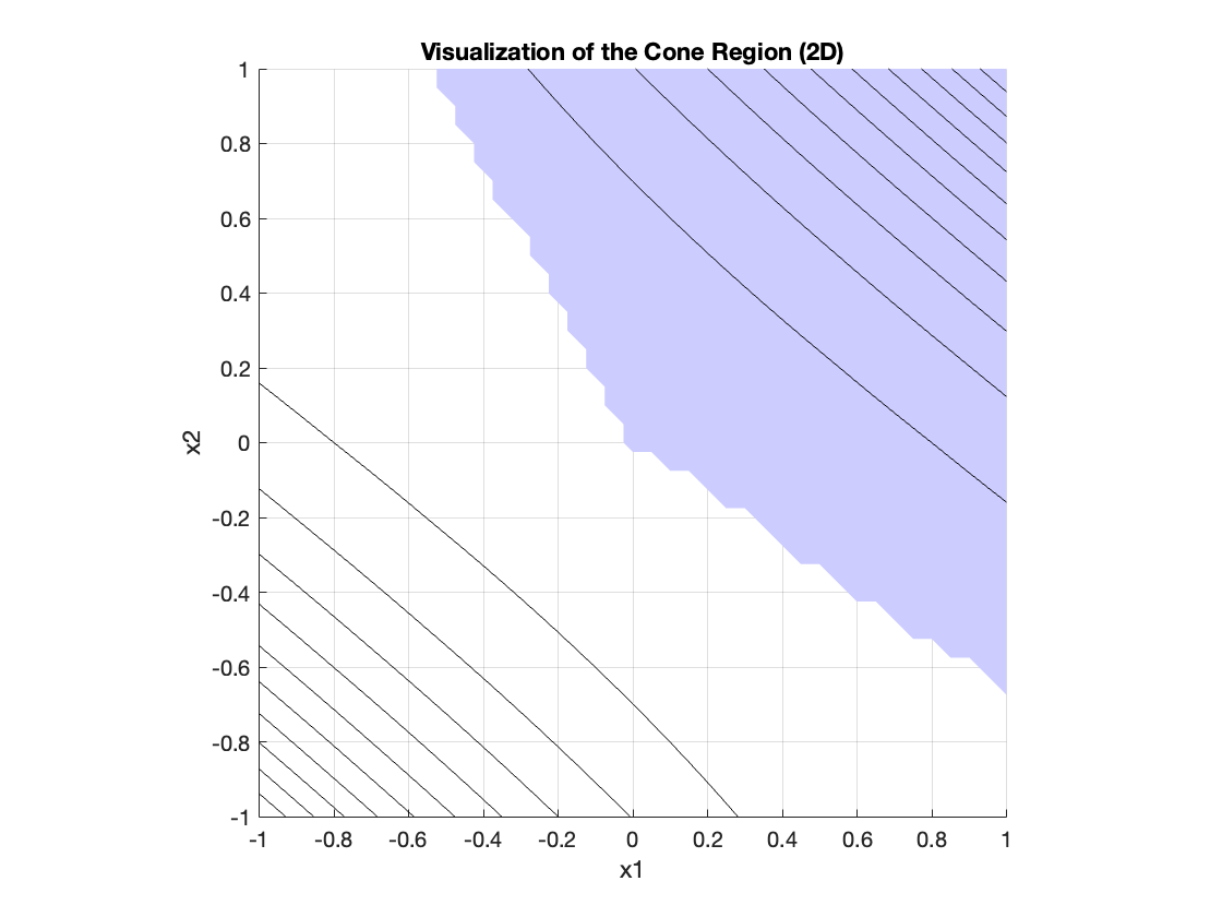
Figure 1. Cone ${\mathcal{K}}={\mathcal{K}}(f,v)$

5.2. Rayleigh-Difference Polynomial

Let $f$ be a multi-affine polynomial. Then $f$ is real stable over the nonnegative orthant if and only if the Rayleigh -Difference polynomial $\Delta_{i,j}f(x):=\partial_{i}f\partial_{j}f-f\partial_{i}\partial_{j}f$ is nonnegative for all $x\in{\mathbb{R}}^{n},i,j\in[n]$ [Theorem 5.6][Brä07]. Here we provide a necessary and sufficient condition for a multi-affine polynomial to be log-concave over a convex cone ${\mathcal{K}}$.

Lemma 5.12.

Let $f$ be a multi-affine polynomial. Then $f$ is log-concave over a convex cone $K$ if and only if $\Delta_{i,j}f(x)$ is nonnegative for all $x\in K,i,j\in[n]$.

Proof.

For any multi-affine polynomial $f$, we have $\Delta_{i,j}f=\left(\frac{\partial f}{\partial x_{i}}\frac{\partial f}{\partial x_{j}}-f.\frac{\partial^{2}f}{\partial x_{i}\partial x_{j}}\right)=-f^{2}\frac{\partial^{2}}{\partial x_{i}\partial x_{j}}\log f$. Therefore, $f$ is log-concave over $K$ if and only if $\frac{\partial^{2}}{\partial x_{i}\partial x_{j}}\log f(x)$ is negative for all $x\in K,i,j\in[n]$ if and only if $\Delta_{i,j}f\geq 0$ for all $x\in K$ and $i,j\in[n]$.

Remark 5.13.

If $f$ is a stable polynomial, the Rayleigh difference polynomial is globally nonnegative. Consequently, by applying Lemma˜5.12, we deduce that $f$ is log-concave over ${\mathbb{R}}^{n}$. Furthermore, since $f$ is stable, it follows that $f$ is hyperbolic with respect to every point in the nonnegative orthant, which implies that $f$ is CLC over the nonnegative orthant. Note that CLC is a stronger property than log-concavity, meaning a stronger condition is required for a multiaffine polynomial to be ${\mathcal{K}}$-CLC.

Note that $\Delta_{v,w}(f):=D_{w}f.D_{v}f-f.D_{w}D_{v}f$ is known as the Rayleigh difference polynomial w.r.t $v,w$, of degree $2d-2$ for any $f\in{\mathbb{R}}^{d}_{n}[x]$. Consider the polynomial $f(x)=-2x_{1}^{3}+12x_{1}^{2}x_{2}+18x_{1}x_{2}^{2}-8x_{2}^{3}$. It’s is hyperbolic w.r.t $(1,1)$. The Rayleigh difference polynomial, $\Delta_{v,w}(f)$, is a quartic bivariate polynomial. Using the Hilbert’s 17-th problem non-negative $\Delta_{v,w}(f)$ is equivalent to a sum of square polynomial. It’s easy to find a positive semidefinite matrix $M$ such that $f=q(x)Mq(x)^{T}$ where $q(x)=\begin{bmatrix}x_{1}^{2}&x_{1}x_{2}&x_{2}^{2}\end{bmatrix}$ denotes the vector monomial.

This technique is known for defining hyperbolicity cones via nonnegative polynomials for any hyperbolic polynomials, see [KPV15] for details.Although the result cannot be extended for ${\mathcal{K}}$-Lorentzian polynomials, meaning let $f(x)\in{\mathbb{R}}^{d}_{n}[x]$ be a ${\mathcal{K}}$-Lorentzian polynomial over the proper convex cone ${\mathcal{K}}$ and $v\in\operatorname{int}{\mathcal{K}}$. Then the Rayleigh difference polynomial $D_{w}f.D_{v}f-f\cdot D_{w}D_{v}f$ need not be nonnegative over ${\mathbb{R}}^{n}$. However, we show that it’s nonnegative over the proper convex cone ${\mathcal{K}}(f,v)$. For instance, consider Example˜5.11. Then Rayleigh difference polynomial w.r.t $v=(1,1)$ and $w=(2,1)$ is $\Delta_{v,w}f(x)=3(119x_{1}^{4}+580x_{1}^{3}x_{2}+1002x_{1}^{2}x_{2}^{2}+768x_{1}x_{2}^{3}+240x_{2}^{4})$, a quartic bivariate polynomial. It’s easy to check using any computer algebra system that there cannot exist any positive semidefinite matrix for which $f=q(x)Mq(x)^{T}$ where $q(x)=\begin{bmatrix}x_{1}^{2}&x_{1}x_{2}&x_{2}^{2}\end{bmatrix}$. Thus, it’s not a SOS polynomial and consequently, not a nonnegative polynomial by Hilbert’s 17th problem. Although, note that $\Delta_{v,w}f(x)$ is nonnegative over the nonnegative orthant. Moreover, $f$ is a $2(1-1/d)$-Rayleigh, i.e., $2(1-1/d)D_{w}f.D_{v}f\geq f\cdot D_{w}D_{v}f$ as proved in [BH20, Prop 2.19]. Note that for this example, the Rayleigh difference polynomial is not nonnegative over ${\mathbb{R}}^{n}$ but it’s nonnegative over ${\mathbb{R}}^{n}_{\geq 0}$. We extend this result for ${\mathcal{K}}$-Lorentzian polynomials.

Theorem 5.14.

let $f(x)\in{\mathbb{R}}^{d}_{n}[x]$ be a ${\mathcal{K}}$-Lorentzian polynomial over the proper convex cone ${\mathcal{K}}$ and $v,w\in{\mathcal{K}}$. Then the Rayleigh difference polynomials $D_{w}f.D_{v}f-f\cdot D_{w}D_{v}f$ are nonnegative over ${\mathcal{K}}$ for all $v,w\in{\mathcal{K}}$.

Proof.

Let $M(x):=\nabla f(x)\nabla f(x)^{t}-f(x)H_{f}(x)$. Since $f$ is ${\mathcal{K}}$-Lorentzian polynomial, the Hessian of $-\log f(x)$, $-H_{\log f}(x)=\frac{M(x)}{f(x)^{2}}$ is positive semidefinite on ${\mathcal{K}}$. Therefore, for any $x\in{\mathcal{K}}$, $M(x)\succeq 0$. Note that for all $v,w\in{\mathcal{K}}$, $M(x)\succeq 0$ on ${\mathcal{K}}\Leftrightarrow\langle v,M(x)w\rangle\geq 0$. Then the rest follows from the fact $v^{t}M(x)w\geq 0$ is equivalent to $D_{v}f(x)D_{w}f(x)-f(x)D_{v}D_{w}f(x)\geq 0$. ∎

5.3. Semipositive cone

Here we are interested to characterize the hyperbolic polynomials whose hyperbolicity cones intersect the positive orthant. We show that when the matrix $A$ is nonsingular and semipositive, the generating hyperbolic polynomials has the desired property. Note that a matrix $A$ is semipositve if there exists $x>0$ such that $Ax>0$. The corresponding semipositive cone is defined as follows.

$$\operatorname{int}K_{A}=\{x\in{\mathbb{R}}^{n}_{>0}:Ax>0\}$$

It’s shown that if $A\in{\mathbb{R}}^{n\times n}$ is semipositive, the closure of $\operatorname{int}K_{A}$, denoted as $K_{A}=\{x\in{\mathbb{R}}^{n}_{\geq 0}:Ax\geq 0\}$ is a proper convex cone in ${\mathbb{R}}^{n}$, cf. [Tsa16]. Furthermore, $K_{A}$ is a polyhedral cone which is obtained as the intersection of two polyhedral cones, specifically, the nonnegative orthant ${\mathbb{R}}^{n}_{+}$ and the cone generated by the columns of $A$.

Proposition 5.15.

The intersection of the hyperbolicity cone $\Lambda_{+}(f_{A},e)$ with the nonnegative orthant is the semipositive cone $K_{A}$ when $f_{A}$ is the generating polynomial of the nonsingular and semipositive matrix $A$.

Proof.

Note that the generating polynomial is a hyperbolic polynomial w.r.t some $e$ by Proposition˜5.9. Moreover, $f_{A}=\det(\sum_{j=1}x_{j}D_{j})$ where diagonal matrices $D_{j}$ are defined by the corresponding $j$-th column of $A$. Thus, it is a determinantal polynomial and the hyperbolicity cone $\Lambda_{+}(f_{A},e)$ is a simplicial cone. More precisely, $\Lambda_{+}(f_{A},e)=\{x\in{\mathbb{R}}^{n}:\sum_{j=1}^{n}x_{j}D_{j}\geq 0\}=\{x\in{\mathbb{R}}^{n}:Ax\geq 0\}$. Hence $\Lambda_{+}(f_{A},e)\cap{\mathbb{R}}^{n}_{\geq 0}=\{x\in{\mathbb{R}}^{n}_{\geq 0}:Ax\geq 0\}=K_{A}$, a proper polyhedral cone. ∎

Corollary 5.16.

Let $A$ be a nonsingular matrix. Then $f_{A}$ is a ${\mathcal{K}}$-Lorentzian (and indeed hyperbolic) polynomial where ${\mathcal{K}}=\Lambda_{+}(f_{A},e)$, a simplicial cone.

Example 5.17.

Consider the matrix outlined in Example˜5.10. Then the corresponding semipositive cone $K_{A}=\{x\in{\mathbb{R}}^{n}_{\geq 0}:Ax\geq 0\}$ is depicted in Figure˜2.

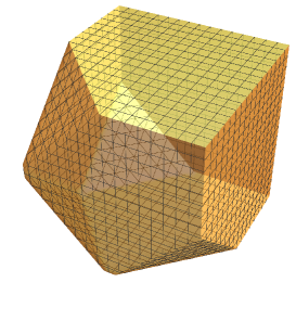
Figure 2. 3D compact base of the cone ${\mathcal{K}}_{A}=\Lambda_{+}(f_{A},1)\cap{\mathbb{R}}^{4}_{\geq 0}$ at $x_{4}=1$

Generalization: ${\mathcal{K}}$-semipositive cone

Here we generalize the notion of semipositive matrices and its corresponding semipositive cone for any proper convex cone ${\mathcal{K}}$ instead of nonnegative orthant. Let ${\mathcal{K}}$ be a proper convex cone. A matrix $A\in{\mathbb{R}}^{n\times n}$ is called ${\mathcal{K}}$-semipositive if it satisfies $Ax\in\operatorname{int}{\mathcal{K}}$ implies $x\in\operatorname{int}{\mathcal{K}}$, i.e., $A(\operatorname{int}{\mathcal{K}})\cap\operatorname{int}{\mathcal{K}}\neq\emptyset$.

Theorem 5.18.

[BP94, Chap-5, Th 5.1] Let ${\mathcal{K}}$ be a proper convex cone.

1. If $A$ is ${\mathcal{K}}$-irreducible and $A({\mathcal{K}})={\mathcal{K}}$, then $A^{-1}$ is also ${\mathcal{K}}$-irreducible and $A(\partial{\mathcal{K}})=A^{-1}(\partial{\mathcal{K}})=\partial{\mathcal{K}}$.

2. Let $A$ be a ${\mathcal{K}}$-nonnegative and ${\mathcal{K}}$-semipositive matrix. Then $A({\mathcal{K}})={\mathcal{K}}$.

As an example, consider $J=\operatorname{Diag}[1,-1,-1,\dots,-1]$, which is ${\mathcal{L}}_{n}$-irreducible and satisfies $J({\mathcal{L}}_{n})={\mathcal{L}}_{n}$ where ${\mathcal{L}}_{n}$ denotes the $n$ dimensional second order cone. We demonstrate that this is not the only such case; one of the key advantages of this type of situation is its significant role in optimization when the feasible set is formed by the intersection of two proper convex cones.

Remark 5.19.

Let $A({\mathcal{K}})={\mathcal{K}}$ where ${\mathcal{K}}$ be a proper convex cone. If $A$ is nonsingular, then both of $A$ and $A^{-1}$ are ${\mathcal{K}}$-nonnegative.

Remark 5.20.

Let $A$ be a nonsingular and ${\mathcal{K}}$-irreducible matrix such that $A({\mathcal{K}})={\mathcal{K}}$. Then the eigenvalues of $A$ have the same modulus. The matrix $A$ in Example˜5.10 satisfies all the conditions over its hyperbolicity cone.

In Example˜5.10, the matrix $A$ is ${\mathcal{K}}$-irreducible and (${\mathbb{R}}^{4}_{\geq 0}$)-semipositive. Therefore, $f_{A}$ is $K_{A}$-Lorentzian on the semipositive cone $K_{A}=\{x\in{\mathbb{R}}^{n}_{\geq 0}:Ax\geq 0\}=\Lambda_{+}(f_{A},e)\cap{\mathbb{R}}^{n}_{\geq 0}$, a proper polyhedral cone. In line with Corollary˜5.16 and Theorem˜5.18 we establish the following.

Theorem 5.21.

Let $A$ be a nonsingular and $\tilde{{\mathcal{K}}}$-semipositive matrix where $\tilde{{\mathcal{K}}}$ is a proper convex cone containing $e$. Then the generating polynomial $f_{A}$ is ${\mathcal{K}}_{A}$-Lorentzian polynomial where $K_{A}:=\Lambda_{+}(f_{A},e)\cap\tilde{{\mathcal{K}}}$, a $\tilde{{\mathcal{K}}}$-semipositive cone.

Proof.

Since $A$ be a nonsingular matrix, so by Corollary˜5.16 the generating polynomial $f_{A}$ is a $\Lambda_{+}(f,e)$-Lorentzian polynomial for some $e\in\Lambda_{+}(f,e)$, a simplicial cone. It’s shown in Proposition˜5.15 that $\Lambda_{+}(f,e)=\{x\in{\mathbb{R}}^{n}:Ax\geq 0\}$. Since $A$ is $\tilde{{\mathcal{K}}}$-semipositive and $e\in\tilde{{\mathcal{K}}}$, so, $f_{A}$ is ${\mathcal{K}}_{A}$- Lorentzian polynomial where ${\mathcal{K}}_{A}:=\{x\in\tilde{{\mathcal{K}}}:Ax\geq 0\}=\Lambda_{+}(f_{A},e)\cap\tilde{{\mathcal{K}}}$, a $\tilde{{\mathcal{K}}}$-semipositive cone. ∎

In [BGLS01, Sec-8] it has been shown that every homogeneous convex cone admits a hyperbolic barrier function. While not every hyperbolicity cone is necessarily a homogeneous cone, the following result illustrates the conditions under which a hyperbolicity cone forms a homogeneous cone.

Example 5.22.

We get $A\left(\Lambda_{+}(f_{A},1)\right)=\Lambda_{+}(f_{A},1)$ for $A$ as discussed in Example˜5.10.

6. Stability Analysis via ${\mathcal{K}}$-Lorentzian polynomials

Lyapunov theorem states that the positive stability of a transformation $A$ is equivalent to the global asymptotic stability of $\frac{dx}{dt}+Ax=0$. A matrix $A$ is stable if every eigenvalue of $A$ has negative real part. If $A$ is a real symmetric matrix, then $A$ is stable if and only if $A$ is negative definite. Lyapunov Theorem asserts that $A$ is positive stable equivalently, $-A$ is stable) if and only if there exists a positive definite matrix $P$ such that the Lyapunov operator $L_{A}:=A^{t}P+PA$ is positive definite. Recall that a real-valued $n\times n$ matrix $A$ is stable if all its eigenvalues belong to the open left half plane.

Theorem 6.1.

Using Routh-Hurwitz criterion, cf., [Poz09, Chap-9] and [JM12, Chap-7], the FAE:

1. The matrix $A$ is stable.

2. The characteristic polynomial $\chi(A)=f(t)$ is Hurwitz-stable polynomial.

3. All the leading principal minors of the corresponding Hurwitz matrix ${\mathrm{Hur}}_{f(t)}$ are positive.

Hence, we have the following.

Theorem 6.2.

Let $f(t)$ be a strictly CLC polynomial of degree $d\leq 4$ for $t\geq 0$. Then the corresponding dynamical system $\frac{dx}{dt}=Ax$ is stable if the characteristic polynomial $\chi(A)=f(t)$.

Proof.

Since $f(t)$ is a strictly CLC polynomial of degree $d\leq 4$ for $t\geq 0$, $f(t)$ is Hurwitz-stable by Theorem˜4.20. Then it follows from Theorem˜6.1. ∎

Corollary 6.3.

Let $f(t)=\sum_{k=0}^{5}a_{k}t^{k}$ be a strictly CLC polynomial of degree $5$ for $t\geq 0$. If $(a_{1}a_{4}-a_{0}a_{5})^{2}<(a_{1}a_{2}-a_{0}a_{3})(a_{3}a_{4}-a_{2}a_{5})$, then the corresponding dynamical system $\frac{dx}{dt}=Ax$ is stable where the characteristic polynomial $\chi(A)=f(t)$.

Proof.

The proof follows from Theorem˜4.18 and Theorem˜6.2. ∎

Theorem 6.4.

Let $f(t)=\sum_{k=0}^{d}a_{k}t^{k},d\geq 5$ be a univariate polynomial with positive coefficients and $a_{k}^{2}>x_{0}a_{k-1}a_{k+1}$ where $x_{0}$ is the unique positive root of the polynomial $x^{3}-x^{2}-2x-1(x_{0}\approx 2.1479)$. Then

1. $f(t)$ is Hurwitz-stable and

2. if the characteristic polynomial $\chi(A)=f(t)$, the corresponding dynamical system $\frac{dx}{dt}=Ax$ is stable.

Furthermore, we extend the result for multivariate polynomials.

Theorem 6.5.

Let $f(x)$ be a strictly ${\mathcal{K}}$-CLC of degree $d\leq 4$ with $v\in\operatorname{int}{\mathcal{K}}$. If the characteristic polynomial $\chi(A)=f(x_{0}+tv)$ for some $x_{0}\in\operatorname{int}{\mathcal{K}}$, the dynamical system $\frac{dx}{dt}=Ax$ is stable.

Proof.

If $f(x)$ is a strictly ${\mathcal{K}}$-CLC of degree $d\leq 4$, then by Theorem˜4.20, $f(x)$ is Hurwitz-stable polynomial over ${\mathcal{K}}$. Then it follows from Definition˜4.5 that univariate restriction $f(x+tv)$ is Hurwitz-stable for any $x,v\in\operatorname{int}{\mathcal{K}}$. Thus, the matrix $A$ is (Lyapunov-type) stable if $\chi(A)=f(x_{0}+tv)$ for $x_{0},v\in\operatorname{int}{\mathcal{K}}$ by Theorem˜4.2. Equivalently, all the leading principal minors of the corresponding Hurwitz matrix ${\mathrm{Hur}}_{f(x_{0}+tv)}$ are positive for any $x_{0},v\in\operatorname{int}{\mathcal{K}}$. ∎

Theorem 6.6.

Let $f(x)$ be a strictly ${\mathcal{K}}$-CLC of degree $d\geq 5$ with $v\in\operatorname{int}{\mathcal{K}}$. If the characteristic polynomial $\chi(A)=f(x_{0}+tv)=\sum_{k=0}^{d}a_{k}t^{k}$ with $a_{k}^{2}>\alpha a_{k-1}a_{k+1}$ where $\alpha$ is the unique positive root of the polynomial $t^{3}-t^{2}-2t-1(\alpha\approx 2.1479)$ for any $x_{0}\in\operatorname{int}{\mathcal{K}}$, the dynamical system $\frac{dx}{dt}=Ax$ is stable.

6.1. Cone-Stability

Consider the linear time invariant system (IVP)

$$\frac{dx(t)}{dt}+Ax(t)=0,x(0)=x_{0}\in{\mathcal{K}}.$$

For example, in $2D$ system, consider $A=\begin{bmatrix}1&2\\ 1&1\end{bmatrix}$ and ${\mathcal{K}}={\mathbb{R}}^{2}_{\geq 0}$, cf. [GB04, Example 1], [STH22, Example 1]. Clearly, $A$ is not a stable matrix, since $\operatorname{eig}(A)=\{1+\sqrt{2},1-\sqrt{2}\}$. Another example in 3D system, let $A=\begin{bmatrix}1&3&2\\ 5&-1&1\\ -3&10&2\end{bmatrix}$ and ${\mathcal{K}}={\mathbb{R}}^{3}_{\geq 0}$. $A$ is not a stable matrix, since $\operatorname{eig}(A)=\{6.2773,-2.1387+1.5087i,-2.1387-1.5087i\}$. Thus, the origin is unstable when systems are not constrained on ${\mathcal{K}}$. It is shown in [GB04], [STH22] that the trivial solution, $0$ is asymptotically stable on ${\mathcal{K}}={\mathbb{R}}^{2}_{\geq 0}$ and ${\mathbb{R}}^{3}_{\geq 0}$ respectively. In essence, the equilibrium point may not be stable in the entire state space, but is stable when the system states are constrained to a cone ${\mathcal{K}}$. Inspired by the evidence of the instances that constraints make the system stable even though the unconstrained system was not, we consider the following class of dynamical systems as outlined in [GB04], [STH22], and references therein.

The notation $C^{0}([t_{0},+\infty);{\mathbb{R}}^{d})$ represents the space of continuous functions defined on the interval $[t_{0},+\infty)$,and taking values in ${\mathbb{R}}^{d}$. The notation $L^{\infty}_{\mathrm{loc}}(t_{0},+\infty;{\mathbb{R}}^{d})$ represents the space of locally essentially bounded functions defined on $(t_{0},+\infty)$ with values in ${\mathbb{R}}^{d}$. The notation $C^{1}({\mathbb{R}}^{d};{\mathbb{R}})$ represents the space of continuously differentiable scalar-valued functions defined on ${\mathbb{R}}^{d}$.

The class of Dynamical Systems: Let ${\mathcal{K}}\subset{\mathbb{R}}^{d}$ be a nonempty closed convex set. Let $A\in{\mathbb{R}}^{d\times d}$ be a given matrix and $F:{\mathbb{R}}^{d}\rightarrow{\mathbb{R}}^{d}$ a nonlinear operator. For $(t_{0},x_{0})\in{\mathbb{R}}\times{\mathcal{K}}$, we consider the following problem $P(t_{0},x_{0})$: Find a function $t\rightarrow x(t)(t\geq t_{0})$ with $x\in C^{0}([t_{0},+\infty);{\mathbb{R}}^{d})$ , and $\frac{dx}{dt}\in L^{\infty}_{\mathrm{loc}}(t_{0},+\infty;{\mathbb{R}}^{d})$ such that

(2) $$\begin{cases}&\langle\frac{dx}{dt}(t)+Ax(t)+F(x(t)),v-x(t)\rangle\geq 0,\ \ \forall v\in{\mathcal{K}},\ \mbox{a.e}\ t\geq t_{0}\\ &x(t)\in{\mathcal{K}},\ \ \ \ t\geq t_{0}\end{cases}$$

$$x(t_{0})=x_{0}.$$

This is known as an evolution variational inequality (EVI) dynamical system. Recall that the normal cone of a closed convex set ${\mathcal{K}}$ at a point $x\in{\mathcal{K}}$ is defined as:

$$N_{{\mathcal{K}}}(x)=\{y\in{\mathbb{R}}^{n}:\langle y,v-x\rangle\leq 0,\forall v\in{\mathcal{K}}\}$$

The tangent cone is the polar of the normal cone:

$$T_{{\mathcal{K}}}(x)=\{d\in{\mathbb{R}}^{n}:\langle d,y\rangle\leq 0,\forall y\in N_{{\mathcal{K}}}\}=\mathrm{cl}\{d\in{\mathbb{R}}^{n}:d=\alpha(v-x),v\in{\mathcal{K}},\alpha\geq 0\}$$

Then, using the standard convex analysis tools one can equivalently rewrite the EVI dynamical system $P(t_{0},x_{0})$ as

$$\begin{cases}\langle\frac{dx}{dt}+Ax+F(x),v-x\rangle\geq 0,\ \forall v\in{\mathcal{K}},\ \mbox{a.e}\ t\geq t_{0}\\ x(t)\in{\mathcal{K}},\ \ t\geq t_{0}\end{cases}\Leftrightarrow\begin{cases}\frac{dx}{dt}+Ax+F(x)\in-N_{{\mathcal{K}}}(x)\\ x(t)\in{\mathcal{K}},t\geq t_{0}\end{cases}$$

Here we mention the conditions for the existence and uniqueness of the initial value problem $P(t_{0},x_{0})$ which is a special case of more general setting outlined in [GMM03, Theorem 2.1-Kato, Cor 2.2].

Theorem 6.7.

[GB04] Let ${\mathcal{K}}\subset{\mathbb{R}}^{d}$ be a nonempty closed convex set of ${\mathbb{R}}^{d}$ and let $A\in{\mathbb{R}}^{d\times d}$ be a real matrix of order $d$. Suppose that $F:{\mathbb{R}}^{d}\rightarrow{\mathbb{R}}^{d}$ can be written as

$$F=F_{1}+\Phi^{{}^{\prime}}$$

where $F_{1}$ is Lipschitz continuous and $\Phi\in C^{1}({\mathbb{R}}^{d};{\mathbb{R}})$ is convex. Let $t_{0}\in{\mathbb{R}}$ and $x_{0}\in{\mathcal{K}}$ be given. Then there exists a unique $x(t):=x(.;t_{0},x_{0})\in C^{0}([t_{0},+\infty);{\mathbb{R}}^{d})$, such that $\frac{dx}{dt}\in L^{\infty}_{\mathrm{loc}}(t_{0},+\infty;{\mathbb{R}}^{d})$, $x$ is right differentiable on $[t_{0},+\infty)$, and the conditions of (2) are satisfied.

Remark 6.8.

Additionally, if it is assumed that $0\in{\mathcal{K}}$ and $\langle F(0),v\rangle\geq 0$ for all $v\in{\mathcal{K}}$, then the unique solution $x(t,t_{0},0)=0$, $t\geq t_{0}$, i.e., the trivial solution $0$ is the unique solution of the problem $P(t_{0},0)$. We consider the class of dynamical system which satisfies all the conditions mentioned in Theorem˜6.7 along with $0\in{\mathcal{K}}$ and $\langle F(0),v\rangle\geq 0$ for all $v\in{\mathcal{K}}$. We refer such systems as $P(t_{0},x_{0})$ throughout the rest of the paper unless stated otherwise.

We now define stability of an equilibrium point w.r.t a closed convex set ${\mathcal{K}}$ for the EVI system as outlined in [GB04], [STH22].

Definition 6.9.

The equilibrium point $x=0\in{\mathcal{K}}$ is called (Lyapunov-type) stable w.r.t ${\mathcal{K}}$ if for any $\epsilon>0$, there exists a $\delta>0$ such that for any initial condition $x_{0}\in{\mathcal{K}}$ with $\|x_{0}\|\leq\delta$, the solution $x(t)\in{\mathcal{K}}$ of the system EVI satisfies $\|x(t)\|<\epsilon$ for all $t\geq t_{0}$. The equilibrium point $x=0\in{\mathcal{K}}$ is called asymptotically stable w.r.t ${\mathcal{K}}$ if it is stable and there exists a $\delta>0$ such that for any $x_{0}\in{\mathcal{K}}$ with $\|x_{0}\|\leq\delta$, the solution $x(t)\in{\mathcal{K}}$ of the EVI system approaches to the origin, i.e., $\lim_{t\rightarrow\infty}\|x(t)\|=0$, equivalently, $\lim_{t\rightarrow\infty}x(t)=0$.

This means that any trajectory within the cone that starts sufficiently close to $0$ remains within a specified distance from $0$ for all future times. In this paper, we assume that ${\mathcal{K}}$ is a proper convex cone. However, these results also apply to any closed convex set ${\mathcal{K}}$ that contains the origin; see [GB04] for details. Here we discuss some results related to ${\mathcal{K}}$-copositive matrices, stability w.r.t ${\mathcal{K}}$, and strictly ${\mathcal{K}}$-CLC. In order to do that we first report some general abstract theorems of stability, asymptotic stability and instability w.r.t ${\mathcal{K}}$ in terms of generalized Lyapunov functions, cf. [GB04].

Theorem 6.10.

Consider a system $P(t_{0},x_{0})$. Suppose there exist $\sigma>0$ and $V\in C^{1}({\mathbb{R}}^{d};{\mathbb{R}})$ such that

1. $V(x)\geq a(\|x\|),\ x\in{\mathcal{K}},\|x\|\leq\sigma$ with $a:[0,\sigma]\rightarrow{\mathbb{R}}$ satisfying $a(t)>0$, for all $t\in(0,\sigma)$;

2. $V(0)=0$;

3. $x-V^{{}^{\prime}}(x)\in{\mathcal{K}}$, for any $x\in\partial{\mathcal{K}}$ and $\|x\|\leq\sigma$ ;

4. $\langle Ax+F(x),V^{{}^{\prime}}(x)\rangle\geq 0$, for all $x\in{\mathcal{K}}$ and $\|x\|\leq\sigma$.

Then, the trivial solution of $P(t_{0},x_{0})$ is stable w.r.t ${\mathcal{K}}$.

Theorem 6.11.

Consider a system $P(t_{0},x_{0})$. Suppose there exist $\lambda>0,\sigma>0$ and $V\in C^{1}({\mathbb{R}}^{d};{\mathbb{R}})$ such that

1. $V(x)\geq a(\|x\|),\ x\in{\mathcal{K}},\|x\|\leq\sigma$ with $a:[0,\sigma]\rightarrow{\mathbb{R}}$ satisfying $a(t)>ct^{\tau}$, for all $t\in[0,\sigma]$, for some constants $c>0,\tau>0$;

2. $V(0)=0$;

3. $x-V^{{}^{\prime}}(x)\in{\mathcal{K}}$, for any $x\in\partial{\mathcal{K}}$ and $\|x\|\leq\sigma$ ;

4. $\langle Ax+F(x),V^{{}^{\prime}}(x)\rangle\geq\lambda V(x)$, for all $x\in{\mathcal{K}}$ and $\|x\|\leq\sigma$.

Then, the trivial solution of $P(t_{0},x_{0})$ is asympotically stable w.r.t ${\mathcal{K}}$.

Remark 6.12.

The condition $(3)$ is a sufficient condition which implies $-V^{{}^{\prime}}(x)\in T_{{\mathcal{K}}}(x)$ for all $x\in\partial{\mathcal{K}}$, $\|x\|\leq\sigma$, where $T_{{\mathcal{K}}}(x)$ is the tangent cone to ${\mathcal{K}}$.

We discuss Lyapunov Stability on ${\mathcal{K}}$ as outlined in [GB04].

Definition 6.13.

The matrix $A\in{\mathbb{R}}^{n\times n}$ is Lyapunov positive stable (semi-stable) on ${\mathcal{K}}$ if there exists a matrix $P\in{\mathbb{R}}^{n\times n}$ such that

1. $\mathrm{inf}_{x\in{\mathcal{K}}\setminus\{0\}}\frac{x^{t}Px}{\|x\|^{2}}>0$;

2. $\langle Ax,[P+P^{t}]x\rangle>0(\geq 0)$ for all $x\in{\mathcal{K}}$;

3. $x\in\partial{\mathcal{K}}\Rightarrow(I-[P+P^{t}])x\in{\mathcal{K}}$.

Let $\mathcal{P}_{{\mathcal{K}}}$ ($\mathcal{P}^{+}_{{\mathcal{K}}}$) denote the set of ${\mathcal{K}}$- copositive (resp. strictly copositive) matrices and

$$\mathcal{P}^{++}_{{\mathcal{K}}}=\{P\in{\mathbb{R}}^{n\times n}:\mathrm{inf}_{x\in{\mathcal{K}}\setminus\{0\}}\frac{x^{t}Px}{\|x\|^{2}}>0\}.$$

Let ${\mathcal{L}}_{k}$ denote the set of all Lyapunov semi-stable matrices on ${\mathcal{K}}$, i.e.,

$${\mathcal{L}}_{{\mathcal{K}}}=\{A\in{\mathbb{R}}^{n\times n}:\exists P\in{\mathcal{P}}^{++}_{{\mathcal{K}}}\ \mbox{such that}\ (I-[P+P^{t}])\partial{\mathcal{K}}\subset{\mathcal{K}}\ \mbox{and}\ A^{t}P+PA\in{\mathcal{P}}_{{\mathcal{K}}}\}$$

and ${\mathcal{L}}^{++}_{k}$ denote the set of all Lyapunov positive stable matrices on ${\mathcal{K}}$, i.e.,

$${\mathcal{L}}^{++}_{{\mathcal{K}}}=\{A\in{\mathbb{R}}^{n\times n}:\exists P\in{\mathcal{P}}^{++}_{{\mathcal{K}}}\ \mbox{such that}\ (I-[P+P^{t}])\partial{\mathcal{K}}\subset{\mathcal{K}}\ \mbox{and}\ A^{t}P+PA\in{\mathcal{P}}^{++}_{{\mathcal{K}}}\}$$

Remark 6.14.

Note that $\langle Ax,[P+P^{t}]x\rangle>0\Leftrightarrow A^{t}P+PA\in{\mathcal{P}}^{++}_{{\mathcal{K}}}$. Let $A\in{\mathbb{R}}^{n\times n}$ be a positive strictly-stable matrix, i.e., the real part of all its eigenvalues are positive. Then there exists a matrix $P$ such that the conditions $(a)$ and $(b)$ in Definition˜6.13 are satisfied since by Lyapunov Theorem there exists a positive definite matrix $P\in{\mathbb{R}}^{n\times n}$ such that $A^{t}P+PA=Q$, a positive definite matrix and $\langle Ax,[P+P^{t}]x\rangle=\langle Qx,x\rangle>0$ for all $x\in{\mathbb{R}}^{d}\setminus\{0\}$.

Lemma 6.15.

[GMM03], [GB04] If ${\mathcal{K}}$ is a proper convex cone, ${\mathcal{P}}^{++}_{{\mathcal{K}}}={\mathcal{P}}^{+}_{{\mathcal{K}}}$.

Furthermore, [GB04, Theorem 5] establishes that in the special case of problem $P(t_{0},x_{0})$ with $F\equiv 0$ referred to as the linear evolution variational inequality (LEVI), Lyapunov stability of matrix $A$ with respect to ${\mathcal{K}}$ can determine the stability of the trivial solution of the $P(t_{0},x_{0})$, LEVI system. Consider LEVI system defined as follows.

(3) $$\begin{cases}\langle\frac{dx}{dt}+Ax,v-x\rangle\geq 0,\ \forall v\in{\mathcal{K}},\ \mbox{a.e}\ t\geq t_{0}\\ x(t)\in{\mathcal{K}},\ \ t\geq t_{0}\end{cases}$$

$$x(t_{0})=x_{0}$$

Theorem 6.16.

[GB04]

1. If $A$ is ${\mathcal{K}}$-copositive, $A$ is Lyapunov semi-stable

2. If $A$ is strictly ${\mathcal{K}}$-copositive, $A$ is Lyapunov positive stable

Proof.

(a) Let $P=\frac{1}{2}I$. Conditions $(a)$ and $(b)$ are straightforward. Additionally, $(A-[P+P^{t}])x=0\in{\mathcal{K}}$. Thus, $A\in L_{{\mathcal{K}}}$.
(b) The choice of $P=\frac{1}{2}I$ still works. ∎

Theorem 6.17.

[GB04, Theorem 5] Let ${\mathcal{K}}$ be a proper convex cone and consider the LEVI system defined in (3). Then

1. If $A\in{\mathcal{L}}_{{\mathcal{K}}}$, then the trivial solution of the LEVI system is stable w.r.t ${\mathcal{K}}$.

2. If $A\in{\mathcal{L}}_{{\mathcal{K}}}^{++}$, then the trivial solution of the LEVI system is asymptotically stable w.r.t. ${\mathcal{K}}$.

Theorem 6.18.

If the quadratic form $x^{t}Ax$ is (strictly)-${\mathcal{K}}$-CLC (equivalently, (strictly) ${\mathcal{K}}$-Lorentzian), then the trivial solution of the LEVI system defined in (3) is (asymptotically) stable w.r.t ${\mathcal{K}}$.

Proof.

If the quadratic form $x^{t}Ax$ is ${\mathcal{K}}$-CLC or strictly ${\mathcal{K}}$-CLC, then the matrix $A$ is ${\mathcal{K}}$-copositive or strictly ${\mathcal{K}}$-copositive, respectively, as stated in Corollary˜2.5. Additionally, if $A$ is ${\mathcal{K}}$-copositive or strictly ${\mathcal{K}}$-copositive, then $A$ is Lyapunov semi-stable or Lyapunov positive stable by Theorem˜6.16. The claim then follows from Theorem˜6.17. ∎

Corollary 6.19.

If the quadratic form $x^{t}Ax$ is (strictly)-${\mathcal{K}}$-CLC, then the trivial solution of the linear autonomous dynamical system of the form $\frac{dx}{dt}+Ax=0$ with $x(t)\in{\mathcal{K}}$ is (asymptotically) stable w.r.t ${\mathcal{K}}$.

Proof.

Note that the linear autonomous dynamical system $\frac{dx}{dt}+Ax=0$ is a special case contained in the general case, LEVI dynamical system. ∎

Here, we illustrate the situation through an example by visualizing the cone and system trajectories using MATLAB simulation.

Example 6.20.

Consider the quadratic form $q=-x_{1}^{2}+2x_{1}x_{2}-x_{2}^{2}+2x_{1}x_{3}+2x_{2}x_{3}-x_{3}^{2}$. It is not Lorentzian, but ${\mathcal{K}}$-Lorentzian where ${\mathcal{K}}={\mathcal{K}}(f,v)$ as shown in Figure˜4. The corresponding system is $\frac{dx}{dt}+Ax=0$ where $A=\begin{bmatrix}-1&1&1\\ 1&-1&1\\ 1&1&-1\end{bmatrix}$. The MATLAB simulation code demonstrates how the trajectories converge to the origin when the initial conditions are selected from the cone.

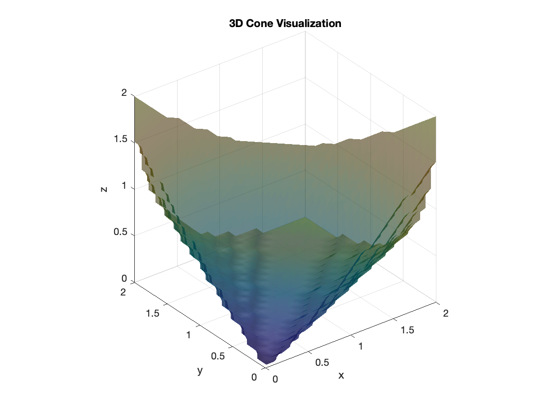
Figure 3. ${\mathcal{K}}={\mathcal{K}}(f,v)$

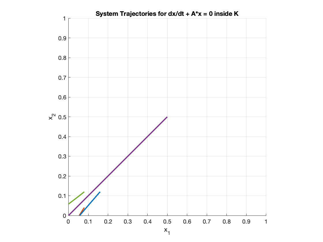
Figure 4. Stability of the origin w.r.t ${\mathcal{K}}$

Corollary 6.21.

If the matrix $A$ is a (positive) nonnegative matrix with exactly one positive eigenvalue, the corresponding LEVI system defined in (3) is (asymptotically) stable over the nonnegative orthant.

Proof.

Note that $A$ is not a positive semidefinite matrix, so the system is not globally asymptotically stable. However, the corresponding quadratic form $x^{t}Ax$ is a (strictly) Lorentzian polynomial by Remark˜2.8. Consequently, it follows from Theorem˜6.18. ∎

Testing whether a quadratic form $q=x^{t}Qx$ is ${\mathcal{K}}$-CLC can be approached in several ways. The characterization of ${\mathcal{K}}$-CLC quadratic forms on three prominent self-dual cones is provided in [BD24]. For the nonnegative orthant (${\mathbb{R}}^{n}_{\geq 0})$, and the Lorentz cone ($\mathcal{L}_{n})$, verifying the ${\mathcal{K}}$-CLC property is relatively simpler compared to testing it over the positive semidefinite (PSD) cone. Let $q$ be a quadratic form on $\mathcal{S}^{n}$ whose matrix $Q$ is nonsingular and has exactly one positive eigenvalue. As shown in [BD24], $q$ is $\mathcal{S}^{n}_{+}$-Lorentzian if and only if the associated quartic polynomial $q(xx^{t})$ is nonnegative for all $x\in\mathbb{R}^{n}$. As a result, determining whether a quadratic form is $\mathcal{S}^{n}_{+}$-Lorentzian is a NP-hard problem, see [BD24] for details.

Now we discuss the case of nonlinear perturbations of LEVI systems. Let ${\mathcal{K}}$ be a proper convex cone. Consider the problem $P(t_{0},x_{0})$: Find $x\in C^{0}([t_{0},+\infty);{\mathbb{R}}^{d})$ where $\frac{dx}{dt}\in L^{\infty}_{\mathrm{loc}}(t_{0},+\infty;{\mathbb{R}}^{d})$ such that

(4) $$\begin{cases}&x(t)\in{\mathcal{K}},\ \ \ \ t\geq t_{0}\\ &\langle\frac{dx}{dt}(t)+Ax(t)+F(x(t)),v-x(t)\rangle\geq 0,\ \ \forall v\in{\mathcal{K}},\ \mbox{a.e}\ t\geq t_{0}\\ \end{cases}$$

$$x(t_{0})=x_{0}$$

Theorem 6.22.

[GB04, Theorem 7] Let ${\mathcal{K}}$ be a proper convex cone. Consider the dynamical system defined in (4), such that $-\Phi^{{}^{\prime}}(0)\in N_{{\mathcal{K}}}(0)$ and $\lim_{\|x\|\rightarrow 0}\frac{\|F_{1}(x)\|}{\|x\|}=0$ where $F=F_{1}+\Phi^{{}^{\prime}}$. If $A\in\mathcal{P}^{++}_{{\mathcal{K}}}$, then the trivial solution of this system is asymptotically stable.

Theorem 6.23.

If the quadratic form $x^{t}Ax$ is (strictly)-${\mathcal{K}}$-CLC, then the trivial solution of the nonlinear perturbed LEVI system defined in (4) is (asymptotically) stable w.r.t ${\mathcal{K}}$.

Proof.

Note that the assumptions $-\Phi^{{}^{\prime}}(0)\in N_{{\mathcal{K}}}(0)$ and $\lim_{\|x\|\rightarrow 0}\frac{\|F_{1}(x)\|}{\|x\|}=0$ ensure that $-F(0)\in N_{{\mathcal{K}}}(0)$, i.e., $\langle F(0),v\rangle\geq 0$ for all $v\in{\mathcal{K}}$. Therefore, the trivial solution $0$ is the unique solution of $P(t_{0},0)$. If the quadratic form $x^{t}Ax$ is (strictly) ${\mathcal{K}}$-CLC, $A$ is (strictly) ${\mathcal{K}}$-copositive by Corollary 2.5. Then the result follows from Theorem˜6.22 ∎

Acknowledgements. I am deeply grateful to Greg Blekherman and Marcella M. Gomez for their valuable suggestions on the earlier version of this article, which significantly contributed to its improvement.

References

- [AGV21] Nima Anari, Shayan Oveis Gharan, and Cynthia Vinzant. Log-concave polynomials, I: entropy and a deterministic approximation algorithm for counting bases of matroids. Duke Math. J., 170(16):3459–3504, 2021.
- [ALOGV24] Nima Anari, Kuikui Liu, Shayan Oveis Gharan, and Cynthia Vinzant. Log-concave polynomials III: Mason’s ultra-log-concavity conjecture for independent sets of matroids. Proc. Amer. Math. Soc., 152(5):1969–1981, 2024.
- [BD24] Grigoriy Blekherman and Papri Dey. -lorentzian polynomials. arXiv preprint arXiv:2405.12973, 2024.
- [BF76] George Philip Barker and James Foran. Self-dual cones in Euclidean spaces. Linear Algebra Appl., 13(1-2):147–155, 1976. Collection of articles dedicated to Olga Taussky Todd.
- [BGLS01] Heinz H Bauschke, Osman Güler, Adrian S Lewis, and Hristo S Sendov. Hyperbolic polynomials and convex analysis. Canadian Journal of Mathematics, 53(3):470–488, 2001.
- [BH20] Petter Brändén and June Huh. Lorentzian polynomials. Annals of Mathematics, 192(3):821–891, 2020.
- [BK64] Richard Ernest Bellman and Robert E Kalaba. Selected papers on mathematical trends in control theory. (No Title), 1964.
- [BK95] Shankar P Bhattacharyya and Lee H Keel. Robust control: the parametric approach. In Advances in control education 1994, pages 49–52. Elsevier, 1995.
- [BL23a] Petter Brändén and Jonathan Leake. Lorentzian polynomials on cones. arXiv preprint arXiv:2304.13203, 2023.
- [BL23b] Petter Brändén and Jonathan Leake. Lorentzian polynomials on cones. arXiv preprint arXiv:2304.13203, 2023.
- [BP94] Abraham Berman and Robert J. Plemmons. Nonnegative matrices in the mathematical sciences, volume 9 of Classics in Applied Mathematics. Society for Industrial and Applied Mathematics (SIAM), Philadelphia, PA, 1994. Revised reprint of the 1979 original.
- [Brä07] Petter Brändén. Polynomials with the half-plane property and matroid theory. Advances in Mathematics, 216(1):302–320, 2007.
- [BS75] GP Barker and Hans Schneider. Algebraic perron-frobenius theory. Linear Algebra and its Applications, 11(3):219–233, 1975.
- [BV04] Stephen P Boyd and Lieven Vandenberghe. Convex optimization. Cambridge university press, 2004.
- [COSW04] Young-Bin Choe, James G Oxley, Alan D Sokal, and David G Wagner. Homogeneous multivariate polynomials with the half-plane property. Advances in Applied Mathematics, 32(1-2):88–187, 2004.
- [G9̈7] Osman Güler. Hyperbolic polynomials and interior point methods for convex programming. Math. Oper. Res., 22(2):350–377, 1997.
- [Gan98] F. R. Gantmacher. The theory of matrices. Vol. 1. AMS Chelsea Publishing, Providence, RI, 1998. Translated from the Russian by K. A. Hirsch, Reprint of the 1959 translation.
- [GB04] Daniel Goeleven and Bernard Brogliato. Stability and instability matrices for linear evolution variational inequalities. IEEE Transactions on Automatic Control, 49(4):521–534, 2004.
- [GMM03] D Goeleven, D Motreanu, and VV Motreanu. On the stability of stationary solutions of first order evolution variational inequalities. Advances in Nonlinear Variational Inequalities, 6(1):01–30, 2003.
- [Gur09] Leonid Gurvits. On multivariate newton-like inequalities. In Advances in combinatorial mathematics, pages 61–78. Springer, 2009.
- [HH69] Emilie Haynsworth and A. J. Hoffman. Two remarks on copositive matrices. Linear Algebra Appl., 2:387–392, 1969.
- [JM12] Rolf Jeltsch and Mohamed Mansour. Stability Theory: Hurwitz Centenary Conference Centro Stefano Franscini, Ascona, 1995, volume 121. Birkhäuser, 2012.
- [KPV15] Mario Kummer, Daniel Plaumann, and Cynthia Vinzant. Hyperbolic polynomials, interlacers, and sums of squares. Mathematical Programming, 153:223–245, 2015.
- [KR48] Mark Grigor’evich Krein and Mark A Rutman. Linear operators leaving invariant a cone in a banach space. Uspekhi mat. nauk, 3(1):3–95, 1948.
- [Kur92] David C. Kurtz. A sufficient condition for all the roots of a polynomial to be real. Amer. Math. Monthly, 99(3):259–263, 1992.
- [KV08] Olga M. Katkova and Anna M. Vishnyakova. A sufficient condition for a polynomial to be stable. J. Math. Anal. Appl., 347(1):81–89, 2008.
- [Lev80] B. Ja. Levin. Distribution of zeros of entire functions, volume 5 of Translations of Mathematical Monographs. American Mathematical Society, Providence, RI, revised edition, 1980. Translated from the Russian by R. P. Boas, J. M. Danskin, F. M. Goodspeed, J. Korevaar, A. L. Shields and H. P. Thielman.
- [LPR05] Adrian Lewis, Pablo Parrilo, and Motakuri Ramana. The lax conjecture is true. Proceedings of the American Mathematical Society, 133(9):2495–2499, 2005.
- [LRS24] Bruno F. Lourenço, Vera Roshchina, and James Saunderson. Hyperbolicity cones are amenable. Math. Program., 204(1-2, Ser. A):753–764, 2024.
- [Poz09] Alexander S Poznyak. Advanced mathematical tools for automatic control engineers: Stochastic techniques. Elsevier Ltd, 2009.
- [Ren04] James Renegar. Hyperbolic programs, and their derivative relaxations. Technical report, Cornell University Operations Research and Industrial Engineering, 2004.
- [STH22] Marianne Souaiby, Aneel Tanwani, and Didier Henrion. Cone-copositive Lyapunov functions for complementarity systems: converse result and polynomial approximation. IEEE Trans. Automat. Control, 67(3):1253–1268, 2022.
- [SV70] Hans Schneider and Mathukumalli Vidyasagar. Cross-positive matrices. SIAM Journal on Numerical Analysis, 7(4):508–519, 1970.
- [Tar18] Pablo Tarazaga. On the structure of the set of symmetric matrices with the perron–frobenius property. Linear Algebra and its Applications, 549:219–232, 2018.
- [Tsa16] MJ Tsatsomeros. Geometric mapping properties of semipositive matrices. Linear Algebra and its Applications, 498:349–359, 2016.
- [Van68] James S. Vandergraft. Spectral properties of matrices which have invariant cones. SIAM J. Appl. Math., 16:1208–1222, 1968.