Analysis of Fluorescence Telescope Data Using Machine Learning Methods

Abstract

Fluorescence telescopes are among the key instruments used for studying ultra-high energy cosmic rays in all modern experiments. We use model data for a small ground-based telescope EUSO-TA to try some methods of machine learning and neural networks for recognizing tracks of extensive air showers in its data and for reconstruction of energy and arrival directions of primary particles. We also comment on the opportunities to use this approach for other fluorescence telescopes and outline possible ways of improving the performance of the suggested methods.

1 Introduction

Fluorescence telescopes (FTs) are an important part of all major modern experiments aimed at studying ultra-high energy cosmic rays (UHECRs, $E\geq 1$ EeV), both the Pierre Auger Observatory [1] and the Telescope Array [2]. FTs register scintillation light emitted from nitrogen molecules in the air excited during the development of extensive air showers (EASs) generated by UHECRs. Measurements are performed in clear moonless nights in the near-UV band. The future cosmic ray observatories are also planned to employ the fluorescence technique, both in ground-based experiments like GCOS [3] and in orbital experiments like K-EUSO [4] or POEMMA [5]. In comparison with surface detectors, be it scintillation detectors of Telescope Array or water tanks of Auger, FTs allow one to estimate energy of primary UHECRs calorimetrically, decreasing the dependence on models of hadronic interactions that cannot be verified experimentally at these energies (see, e.g., [1] for details).

However, both Auger and Telescope Array experiments employ large, expensive telescopes. Another approach, based on using small and comparatively cheap FTs is being developed since mid-2010s: these are the FAST [6] and CRAFFT projects [7] that develop telescopes with an aperture around 1 m². Besides this, a small EUSO-TA telescope built by the JEM-EUSO collaboration has been in operation at the Telescope Array site since 2015 [8]. Using the Telescope Array trigger, it demonstrated the ability to register cosmic rays with energies at around 1 EeV and higher.

Besides their main purpose, FTs have proved to be multi-purpose instruments that can be used to register other fast phenomena that manifest themselves via UV emission in the atmosphere. In particular, they are used by the Auger collaboration to study ELVEs [9] and by the Telescope Array to study terrestrial gamma-ray flashes [10]. The first orbital FT, TUS, was also able to register flashes of multiple different types [11]. Besides this, the joint Russian-Italian fluorescence telescope Mini-EUSO (“UF atmosfera” in the Russian Space Program) has been in operation onboard the International Space Station since 2019, creating a UV map of the nocturnal atmosphere of the Earth but also registering meteors, transient luminous events and other phenomena [12, 13]. All these considerations, together with the current state of the future orbital missions, made us consider the scientific potential of a small FT of the EUSO-TA type in terms of recognizing tracks of EASs and the following reconstruction of energy and arrival directions of primary UHECRs, see also [14]. Using model data, we developed a few methods based on machine learning and neural networks to solve the two tasks. In what follows, we describe the main ideas of the approach, the difficulties we had to overcome, and outline possible directions of the further improvement of the suggested methods.

2 The EUSO-TA Telescope and Simulated Data

EUSO-TA is a refractor type telescope equipped with two Fresnel lenses with a diameter of 1 m each, and a concave focal surface (FS) built of $48\times 48$ pixels. The total field of view (FoV) of the instrument is $10.5^{\circ}\times 10.5^{\circ}$, and the time resolution (also called gate-time unit, GTU) equals 2.5 $\mu$s. Each record consists of 128 data frames of the size of $48\times 48$ (“snapshots” of the focal surface) written each GTU. The telescope can operate at different elevation angles. A detailed description of EUSO-TA can be found in [8].

To create data sets for training and testing our models, we employed CONEX [15] and EUSO-$\overline{\rm Off}$$\underline{\rm line}$ codes [16]. The first program was used to simulate EASs produced by proton primaries in the energy range 5–100 EeV distributed uniformly vs. azimuth angles and proportionally to $\cos\theta$ for zenith angles $0^{\circ}$–$70^{\circ}$. QGSJETII-04 [17] was chosen as a model of hadronic interactions. EUSO-$\overline{\rm Off}$$\underline{\rm line}$ was used to simulate the detector response. The shower cores were put within the projection of the FoV of EUSO-TA on the ground. The distance between shower cores and the telescope varied from 2 km to 40 km, depending on the energy of primary particles. Uniform background illumination had an average rate of 1 photon count per pixel per GTU, as is typical in real observations during moonless nights. We tried data sets with energy distributed quasi-uniformly and log-uniformly. Neither of the two methods demonstrated superiotity in terms of the accuracy of energy reconstruction.

Simulated signals used in our models were requested to produce software triggers. No other quality cuts were applied to the data set, except omitting signals that had just a few hit pixels in one of the corners of the telescope FS. In particular, we did not demand that tracks contained intervals with the shower maximum, even though this can strongly improve the accuracy of energy reconstruction.

3 Track Recognition

The problem of recognizing hit pixels of tracks produced by EASs can be considered as semantic segmentation, i.e., a computer vision task that assigns a class label to each pixel of an image. We are only interested in finding two classes (types) of pixels: those that form a track and all the rest. In [18], we presented a solution of this task based on a convolutional encoder-decoder. Here we show a totally different approach, based on “classical” machine learning methods that do not have some shortcomings of neural networks [19].

The main and most common method of classical machine learning for classification and regression problems is gradient boosting. It is based on reducing the error by constructing an ensemble of simple models (most often decision trees), each of which at a new step tries to reduce the error of the previous step [20]. Gradient boosting has the following advantages:

• it does not require designing the model architecture;

• it does not require data normalization;

• it works with categorical factors;

• it does not require graphics accelerators for training and inference.

In particular, our experiment was run on a basic version of Google Colab with an Intel Xeon CPU with two vCPUs and 13 GB of RAM.

The track segmentation model on a separate frame is a gradient boosting model that solves the problem of binary classification. That is, for each pixel, based on the factors collected for it, it predicts an estimate of the probability that this particular pixel on the current frame is a part of the track. Thus, each data record consisting of 128 frames of the size of $48\times 48$ generates almost 295 thousand potential points for training. However, a major part of the frames does not contain a track and therefore can be excluded from training. In frames where a track is present, it usually occupies 1–10% of all pixels in the frame.

Data for the model was sampled from the original data set as follows:

1. The size of the sample (the number of events) for the model was chosen.

2. In each event, only those frames where the proportion of hit pixels was greater than 1% of the total were selected.

3. The value of photon counts in each pixel was normalized (divided) by the maximum value in the frame.

4. Track labels were modified: pixels with relative normalized values less than 0.25 were excluded from the list of hit pixels.

5. Factors were generated for pixels in each frame.

6. The pixels were randomly divided into training, validation, and testing samples in the ratio of 60/20/20.

The factors for the model are various filters from the OpenCV library [21] that are applied to each frame and transform the value of the signal in each pixel according to a certain rule. Standard linear and inverse transformations were selected as filters, the parameters for which were chosen basing on preliminary training (on 1–2 examples). A visual representation of the filters that were used further in the model can be seen in Fig. 1. An in-depth discussion of image filtering can be found in [22].

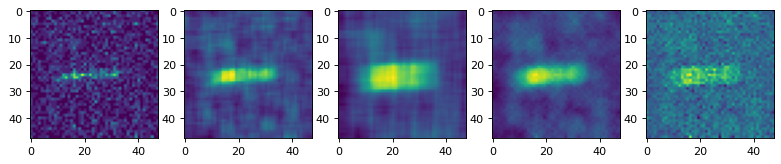
Figure 1: Visual representation of the generated features. From left to right: the initial signal with background illumination, 5-neighbor average, 10-neighbor average, a bilateral filter, and an inverse bilateral filter.

After creating the samples, parameters for the boosting algorithm (XGBoost) were set. Gradient boosting can not build connections between points on a model level as convolutional neural networks do. Instead, for each pixel and each GTU it relies on seven numbers. These are a label assigned to the pixel and six features: four different filterings as shown in Fig. 1, the maximum photon count in the data frame for this particular GTU, and the photon count in the pixel normalized by the maximum value in the frame. Thus, the model does not need to see the whole frame at once to process connections between pixels, and therefore the pixel-level sampling was implemented.

Data from the training and validation samples were fed to the model to control overfitting. Metrics were calculated on the test data. Next, to translate the probability estimates into binary labels, the optimal cutoff was selected: various cutoff values from 0 to 1.0 with a step of 0.01 were considered and the value equal to 0.67 giving the maximum F1-score on the test data was determined. An example of applying the model to a data frame can be seen in Fig. 2. More details about methods of selecting a cutoff can be found in [23].

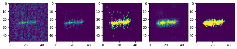
Figure 2: The track recognition model in action. From left to right: the initial signal with background illumination, the same signal with the background removed, the focal surface with hit pixels (yellow) and all the rest, predicted probabilities for the FS pixels to belong to the track, recognized hit pixels (yellow).

To determine the optimal parameters, several versions of the models were trained, in which the number of iterations and the size of the training sample were sequentially increased. Our tests have revealed that a reasonable balance between the time necessary for training the model and the values of metrics that characterize its performance is reached for samples that include just 2000 events. The final model had the following parameters: the number of trees and the maximum tree depth were equal to 3000 and 3 respectively. The learning rate was chosen to be 0.05.

Two performance metrics that are often used in tasks of image recognition to evaluate the accuracy of models are the area under the precision-recall curve (PR AUC) and the balanced accuracy, which is just the mean of the true positive and true negative rates. Our model demonstrated PR AUC and the balanced accuracy equal to 0.900 and 0.898 respectively. These values are slightly lower than 0.958 and 0.949 obtained with the convolutional encoder-decoder, but they needed 16 times less sample size to train the model. This significantly lowers demands on computing resources and also suggest a way for training similar models with limited training samples.

4 Reconstruction of Energy and Arrival Directions

The conventional procedure of reconstructing an event registered with a fluorescence telescope begins with the determination of the shower-detector plane (SDP), see, e.g., [24]. The accuracy of finding the SDP depends on a number of factors, among them the length of the track on the FS of the detector. Next, the shower axis is reconstructed using the timing information from hit pixels. Finally, after the shower geometry is defined, reconstruction of energy becomes possible taking into account all contributing light sources (fluorescence and Cherenkov light, multiple-scattered light) and necessary corrections for “invisible energy” carried away by neutrinos and high-energy muons. Still, it should be remarked that the accuracy of monocular reconstruction is limited even with huge FTs at the Auger and Telescope Array installations when the measured angular speed does not change much over the observed track length. This can be the case, e.g., for short tracks. That is why the best results are usually obtained when data of fluorescence telescopes are combined with information from surface detectors (so called hybrid reconstruction). In this case, the energy resolution of the Auger FT defined as event-to-event statistical uncertainty equals 10% [24].

For EUSO-TA, the task of energy reconstruction is complicated by its small field of view, so that only a small part of a shower track is available in a typical record, see a detailed discussion in [25]. Due to its comparatively coarse time resolution (2.5 $\mu$s compared to 100 ns for the Auger and Telescope Array FTs), data records of EUSO-TA have less accurate information on the temporal development of EAS. It should also be remarked that luminosity of a shower signal in a ground-based FT strongly depends on the distance from the telescope to the shower axis. As a result, a shower originated from a strong but distant EAS can be dimmer than a nearby shower generated by a less energetic primary.

In 2023, we developed a simple 6-layer convolutional neural network (CNN) [26] for reconstructing energy of events registered by the fluorescence telescope of the stratospheric EUSO-SPB2 experiment [27]. It demonstrated decent accuracy with the mean absolute percent error (MAPE) of the order of 10% when just integrated tracks were used as input data. However, the timing information is crucial for a successful reconstruction of events registered by a ground-based FT. This applies to estimating both energy and arrival directions because “flat” images of integrated tracks do not allow one to determine neither real luminosity of an extensive air shower, nor its azimuth with respect to the telescope.

This suggested arranging input data in the form of a “stack” of images of the focal surface. Each image represented a “screenshot” of the FS at one particular GTU. Thus, a sequence of images made at consecutive moments of time provided information about the temporal development of events. The simulated data had trigger GTUs near the beginning of records. Our tests demonstrated that in most cases it is sufficient to utilize data of the first 12 GTUs, thus strongly reducing demands on the amount of memory needed for model training.

The initial CNN developed for EUSO-SPB2 was optimized to use more complex data representation necessary for EUSO-TA. The data set used for training the neural network consisted of 52 thousand events with 20% of them acting as a validation set. All data records were linearly scaled so that the brightest signal was equal to 1. As a result, we were able to teach the CNN to reconstruct both energy and arrival directions of the simulated events. The loss function, which is needed at the stage of training, was chosen according to the reconstructed parameters. The MAPE was employed when energy was the only parameter to be reconstructed. In other cases, we used either mean squared error or mean absolute error. Angular separation complemented one of the two functions in case we were only interested in reconstructing arrival directions. It is interesting to mention that, contrary to the conventional approach, we do not need to determine the shower geometry before reconstructing the energy of a primary particle. The CNN is able to reconstruct energy independently of the arrival direction, and vice versa, as well as it is able to solve both tasks simultaneously.

The trained models were tested on data sets that included 200–500 events from the whole range of energies and arrival directions. In a typical test, energy was reconstructed with MAPE in the range 15–20%, see an example in Fig. 3. The mean error was around 1% with the standard deviation $\sim 20\%$. The largest errors as expressed in MAPE were observed for events at the lower end of energies and arriving from directions nearly orthogonal to the axis of the field of view of EUSO-TA due to the signal being confined to mere 1-2 GTUs of the respective record.

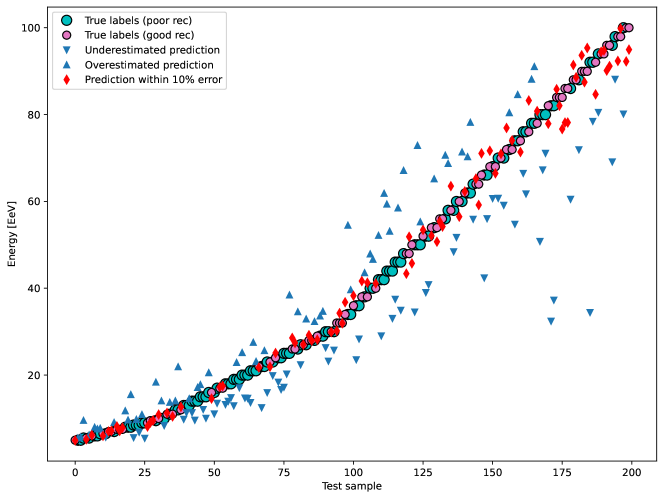
Figure 3: Example of energy reconstruction for EUSO-TA on a test sample consisting of 200 events with energies in the range 5–100 EeV. Circles: true (simulated) energies of primary protons, diamonds: predicted energies with the absolute percentage error $<10\%$, triangles: other predictions. MAPE equals 17.7% in this test.

Zenith and azimuth angles were reconstructed with mean errors $\leq 0.5^{\circ}$ and standard deviations of the order of $4^{\circ}$–$5^{\circ}$ and $15^{\circ}$ respectively. The median value of angular separation between true and reconstructed arrival directions was typically around $4^{\circ}$–$5^{\circ}$. Expectedly, the largest errors took place for events with azimuth angles nearly orthogonal to the axis of the FoV and for events touching only the very corners of the focal surface. Azimuth angles that were along the axis of the telescope $\pm 20^{\circ}$ were reconstructed with the least errors. Fig. 4 presents a typical distribution of angular separation between true and reconstructed arrival directions.

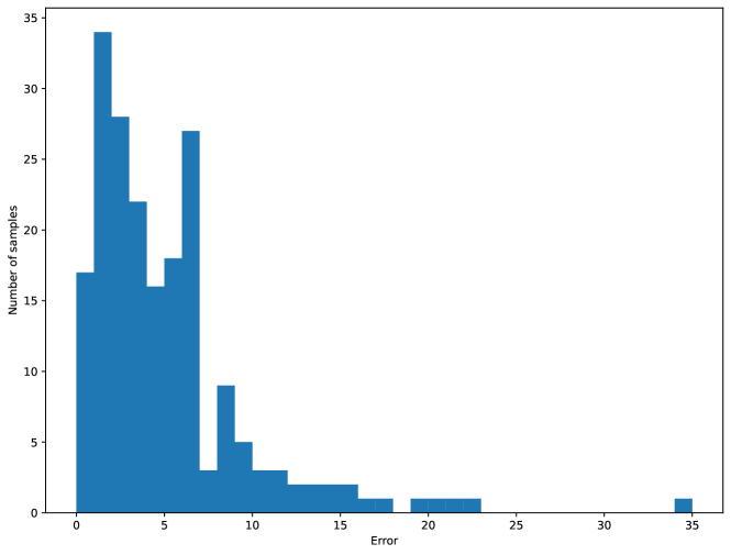
Figure 4: Angular separation between true (simulated) and reconstructed arrival directions for the same sample as in Fig. 3. Errors are expressed in degrees. The median error equals $3.9^{\circ}$.

5 Discussion and Conclusions

We have developed a proof-of-concept convolutional neural network, which is able to reconstruct energy and arrival directions of UHECRs for a small ground-based fluorescence telescope EUSO-TA using simulated data. The same CNN is able to solve this task for the FT pointed in nadir from a stratospheric instrument EUSO-SPB2. The accuracy of reconstruction cannot be directly compared with the much more sophisticated and large FTs working at Pierre Auger Observatory and the Telescope Array, but we think the first results are promising and can be further improved. In particular, models can be trained on a virtual focal surface which is much larger than the real one to teach the neural network to reconstruct missing information from tracks that otherwise hit just a few pixels. More obvious ways of improving the results are to increase the size of the training data set, to tune the hyperparameters of the CNN, to perform training on subsets of the energy range and arrival directions, etc.

We have also developed two methods of recognizing EAS tracks in the focal surface of fluorescence telescopes of both EUSO-TA and EUSO-SPB2. One of them employs gradient boosting, one of the well-known methods of classical machine learning. The second one uses a convolutional encoder-decoder, i.e., an artificial neural network with a special architecture. Both methods demonstrated accuracy $\gtrsim 0.9$ with the neural network performing slightly better. However, the method based on gradient boosting needed a considerably smaller training set and put lower demands on computing resources.

We believe that the suggested methods for EAS track recognition and for reconstruction of energy and arrival directions of primary ultra-high energy cosmic rays are generic and can be applied to other fluorescence telescopes though the architecture of the neural networks will probably need certain modifications to take into account features of a particular instrument.

Funding: M.Z. is supported by grant 22-62-00010 from the Russian Science Foundation.

References

- [1] The Pierre Auger Collaboration, Nuclear Instruments and Methods in Physics Research A 798, 172 (2015). https://doi.org/10.1016/j.nima.2015.06.058
- [2] T. Abu-Zayyad, R. Aida, M. Allen et al., Nuclear Instruments and Methods in Physics Research A 689, 87 (2012). https://doi.org/10.1016/j.nima.2012.05.079
- [3] J.R. Hörandel, in Proc. 37th International Cosmic Ray Conference, Berlin, Germany, PoS 395, 27 (2021). https://doi.org/10.22323/1.395.0027
- [4] P. Klimov, M. Battisti, A. Belov et al., Universe 8, 88 (2022). https://doi.org/10.3390/universe8020088
- [5] A.V. Olinto, J. Krizmanic, J.H. Adams et al., Journal of Cosmology and Astroparticle Physics 2021, 007 (2021). https://doi.org/10.1088/1475-7516/2021/06/007
- [6] M. Malacari, J. Farmer, T. Fujii et al., Astroparticle Physics 119, 102430 (2020). https://doi.org/10.1016/j.astropartphys.2020.102430
- [7] Y. Tameda, T. Tomida, M. Yamamoto et al., Progress of Theoretical and Experimental Physics 2019, 043F01 (2019). https://doi.org/10.1093/ptep/ptz025
- [8] J.H. Adams, S. Ahmad, J.-N. Albert et al., Experimental Astronomy 40, 301 (2015). https://doi.org/10.1007/s10686-015-9441-6
- [9] A. Tonachini for the Pierre Auger Collaboration, Proc. 33rd International Cosmic Ray Conference, Rio de Janeiro, Brazil, 0676 (2013).
- [10] J. W. Belz, P. R. Krehbiel, J. Remington et al., JGR Atmospheres 125, e2019JD031940 (2020). https://doi.org/10.1029/2019JD031940
- [11] P. Klimov, S. Sharakin, M. Zotov, M.E. Bertaina and F. Fenu, Proc. 37th International Cosmic Ray Conference, Berlin, Germany, PoS 395, 316 (2021). https://doi.org/10.22323/1.395.0316
- [12] S. Bacholle, P. Barrillon, M. Battisti at al., Astrophysical Journal Supplement Series 253, 36 (2021). https://doi.org/10.3847/1538-4365/abd93d
- [13] D. Barghini, M. Battisti, A. Belov et al., Astronomy & Astrophysics 687, A304 (2024). https://doi.org/10.1051/0004-6361/202449236
- [14] P. Klimov, A. Belov, M. Zotov, S. Sharakin, D. Chernov, “Concept of a small fluorescence telescope for registering extensive air showers,” report at the 38th Russian Cosmic Ray Conference (2024).
- [15] T. Bergmann, R. Engel, D. Heck, N. Kalmykov, S. Ostapchenko, T. Pierog, T. Thouw, and K. Werner, Astroparticle Physics 26, 420 (2007). http://dx.doi.org/10.1016/j.astropartphys.2006.08.005
- [16] S. Abe, J.H. Adams, D. Allard et al., Journal of Instrumentation 19, P01007 (2024). https://dx.doi.org/10.1088/1748-0221/19/01/P01007
- [17] S. Ostapchenko, Nuclear Physics B Proceedings Supplements 151, 143 (2006). https://doi.org/10.1016/j.nuclphysbps.2005.07.026
- [18] M. Zotov, arXiv:2408.02440 (2024).
- [19] N. O’ Mahony, S. Campbell, A. Carvalho, S. Harapanahalli, G. Velasco-Hernandez, L. Krpalkova, D. Riordan and J. Walsh, in Advances in Computer Vision Proceedings of the 2019 Computer Vision Conference (CVC). Springer Nature Switzerland AG, pp. 128-144 (2020). https://doi.org/10.1007/978-3-030-17795-9
- [20] A. Natekin and A. Knoll, Frontiers in Neurorobotics 7, 21 (2013). https://doi.org/10.3389/fnbot.2013.00021
- [21] G. Bradski, Dr. Dobb’s Journal of Software Tools, 2236121 (2000). https://opencv.org
- [22] B. Desai, M. Paliwal, K.K. Nagwanshi, arXiv:2207.06481 (2022).
- [23] L. Ferrer, arXiv:2209.05355 (2022).
- [24] J. Abraham, P. Abreu, M. Aglietta et al., Nuclear Instruments and Methods in Physics Research A 620, 227 (2010). https://doi.org/10.1016/j.nima.2010.04.023
- [25] J.H. Adams, L. Anchordoqui, D. Barghini et al. Astroparticle Physics 163, 103007 (2024). https://doi.org/10.1016/j.astropartphys.2024.103007
- [26] G. Filippatos and M. Zotov, in Proc. 38th International Cosmic Ray Conference, Nagoya, Japan, PoS 444, 234 (2023). https://doi.org/10.22323/1.444.0234
- [27] J.H. Adams, D. Allard, P. Alldredge et al., Astroparticle Physics 165, 103046 (2024). https://doi.org/10.1016/j.astropartphys.2024.103046