Improving the stability and efficiency of high-order operator-splitting methods

Abstract

Operator-splitting methods are widely used to solve differential equations, especially those that arise from multi-scale or multi-physics models, because a monolithic (single-method) approach may be inefficient or even infeasible. The most common operator-splitting methods are the first-order Lie–Trotter (or Godunov) and the second-order Strang (Strang–Marchuk) splitting methods. High-order splitting methods with real coefficients require backward-in-time integration in each operator and hence may be adversely impacted by instability for certain operators such as diffusion. However, besides the method coefficients, there are many other ancillary aspects to an overall operator-splitting method that are important but often overlooked. For example, the operator ordering and the choice of sub-integration methods can significantly affect the stability and efficiency of an operator-splitting method. In this paper, we investigate some design principles for the construction of operator-splitting methods, including minimization of local error measure, choice of sub-integration method, maximization of linear stability, and minimization of overall computational cost. We propose a new four-stage, third-order, 2-split operator-splitting method with seven sub-integrations per step and optimized linear stability for a benchmark problem from cardiac electrophysiology. We then propose a general principle to further improve stability and efficiency of such operator-splitting methods by using low-order, explicit sub-integrators for unstable sub-integrations. We demonstrate an almost 30% improvement in the performance of methods derived from these design principles compared to the best-known third-order methods.

65L05, 65L06, 65L20

1 Introduction

Operator splitting is a popular approach to solving multi-physics problems. This approach splits the original differential equation into several operators, integrates each operator with an appropriate method, and composes the solutions from the sub-integrations to obtain a solution to the original problem. Generally speaking, any approach that involves distinct treatments of the operators, such as additive, partitioned, or implicit-explicit (IMEX) methods [33, 1, 15, 23, 26], can be considered to be a form of operator splitting. In this paper, we focus on compositional operator-splitting methods [12], also referred to as fractional-step methods [33, 31, 26](see also Eq. 6 below).

A fundamental difference between fractional-step methods and implicit-explicit (IMEX) methods or other additive methods is that in the case of fractional-step methods, each subsystem (fractional step) is integrated independently. The coupling between subsystems occurs only through the initial conditions used for the sub-integrations. In the case of additive methods, the sub-integrations have a stronger coupling. Fractional-step methods are in fact a special case of additive methods [26].

Consider a $2$-additively split ordinary differential equation (ODE)

(1) $$\derivative{y}{t}=\mathcal{F}(t,y)=\mathcal{F}^{[1]}(t,y)+\mathcal{F}^{[2]}(t,y).$$

Let $\displaystyle D^{[\ell]}=\sum\limits_{j}\mathcal{F}^{[\ell]}_{j}(y)\partialderivative{y_{j}}$ be the Lie derivative of $\mathcal{F}^{[\ell]}$. Let $\varphi_{t}^{[\ell]}$ be the exact flow of

(2) $$\derivative{y^{[\ell]}}{t}=\mathcal{F}^{[\ell]}(t,y^{[\ell]}),\quad\ell=1,2.$$

It can be shown that $\varphi_{t}^{[\ell]}(y_{0})=\exp(\Delta tD^{[\ell]})\text{Id}(y_{0})$ and the exact solution of the original differential equation Eq. 1 is $\Phi_{\Delta t}(y_{0})=\exp(\left(D^{[1]}+D^{[2]}\right)\Delta t)\text{Id}(y_{0})$ [12].

A popular method to approximate $\Phi_{\Delta t}(y_{0})$ by solving the subsystems Eq. 2 is

(3) $$\Phi_{\Delta t}(y_{0})=\exp(\left(D^{[1]}+D^{[2]}\right)\Delta t)\text{Id}(y_{0})\approx\exp(D^{[2]}\Delta t)\exp(D^{[1]}\Delta t)\text{Id}(y_{0}).$$

This method can be written as

(4) $$\Psi_{\Delta t}^{\text{LT}}=\varphi_{\Delta t}^{[2]}\circ\varphi_{\Delta t}^{[1]}$$

and is known as the Lie–Trotter (or Godunov) method [30, 9].

Another highly popular method operator-splitting method is the Strang (Strang–Marchuk) method [27, 18] defined as

(5) $$\Psi_{\Delta t}^{\text{S}}=\varphi_{\Delta t/2}^{[1]}\circ\varphi_{\Delta t}^{[2]}\circ\varphi_{\Delta t/2}^{[1]}.$$

Given a set of coefficients $\{\alpha_{k}^{[\ell]}\}_{k=1,2,\dots,s}^{\ell=1,2}$, we define a general $s$-stage, 2-split fractional-step method for solving Eq. 1 as

(6) $$\Psi_{\Delta t}=\varphi_{\alpha_{s}^{[2]}\Delta t}^{[2]}\circ\varphi_{\alpha_{s}^{[1]}\Delta t}^{[1]}\circ\varphi_{\alpha_{s-1}^{[2]}\Delta t}^{[2]}\circ\varphi_{\alpha_{s-1}^{[1]}\Delta t}^{[1]}\circ\cdots\circ\varphi_{\alpha_{1}^{[2]}\Delta t}^{[2]}\circ\varphi_{\alpha_{1}^{[1]}\Delta t}^{[1]},$$

where a stage is defined as a set of sub-integrations through the complete sequence of operators, in this case $\{1,2\}$. In other words, at each stage $k$, the subsystems Eq. 2 are integrated over a time step $\alpha_{k}^{[\ell]}\Delta t$, for $\ell=1,2$, using the solution from the previous sub-integration as the initial condition.

The integration of fractions of the right-hand side generally introduces a splitting error that is in addition to truncation errors from the sub-integrations or roundoff errors. For example, the Lie–Trotter method Eq. 4 is first-order accurate in the sense that the splitting error is $\mathcal{O}(\Delta t)$. The Strang method Eq. 5 is second-order.

In general, one way to construct high-order methods is by choosing the coefficients $\alpha_{k}^{[\ell]}$ satisfy order conditions [14, 2, 3]. Another way is by composing low-order methods [34, 12, 14]. Once a method is found for a given order, its adjoint, i.e., the inverse map with the time direction reversed, also has the same order [12, Theorem 3.1]. When discussing the existence of a given method below, we omit explicitly mentioning the adjoint as a distinct method.

Operator-splitting methods of order three or greater, however, require backward-in-time integration for each operator [10]. These backward integrations can be unstable for certain types of operators, e.g., diffusion, that are not time-reversible. This instability has undoubtedly been a deterrent to trying high-order methods in applications for systems that are not time-reversible. Nonetheless, stability and convergence are possible despite the presence of some instability [5, 26, 32].

There are many other ancillary considerations as well that go into the overall design, implementation, and ultimately performance of an operator-splitting method. For example, one must also select the sub-integration methods. One can use the exact solution of a subsystem Eq. 2, if available (and desirable), or approximate the solution using a numerical method. In this paper, we focus on the family of operator-splitting methods that uses Runge–Kutta methods as sub-integrators. These operator-splitting methods are fractional-step Runge–Kutta (FSRK) methods [26]. The stability function of an $N$-split FSRK method is presented in [26]; here, we present the special case of $N=2$ operators.

Let $R_{k}^{[\ell]}(z)$ be the stability function of the Runge–Kutta method applied to operator $\mathcal{F}^{[\ell]}$ at stage $k$, the stability function of the resulting FSRK method is

(7) $$R\left(z^{[1]},z^{[2]}\right)=\prod\limits_{k=1}^{s}R_{k}^{[1]}\left(\alpha_{k}^{[1]}z^{[1]}\right)R_{k}^{[2]}\left(\alpha_{k}^{[2]}z^{[2]}\right).$$

Equation 7 shows that the stability function of the FSRK method is the product of the stability functions of each Runge–Kutta method with argument, however, scaled by the operator-splitting method coefficient $\alpha_{k}^{[\ell]}$. This interpretation generally holds for $N$ operators. Equation 7 implies that the stability of an FSRK method is generally affected by the ordering of the operators because the arguments are operator-dependent, as well by the method coefficients $\alpha_{k}^{[\ell]}$ themselves and the choice of sub-integration methods.

Although it is clear that different operator-splitting methods perform differently, it is less clear exactly how performance is impacted by the choice of the method coefficients. It is shown in [25] that methods with a good balance between accuracy and cost per step are more efficient, especially when the splitting error is the dominant source of error. Also when using operator-splitting methods, it is also unclear what effect the ordering of the operators has on the performance of the overall method. For example, changing the ordering of the operators in the Lie–Trotter method does not affect the linear stability according to Eq. 7, nor does it generally affect the overall computation time per step because each operator is integrated over the same step-size $\Delta t$; however, the splitting errors are generally different (albeit trivially in this case). It is also straightforward to see that changing the ordering of operators for the Strang method can make a difference in computational efficiency if one operator is significantly more expensive than the other(s) [25]. For $2$-split palindromic methods, changing the order of operators makes no difference in stability; however, the accuracy can vary. In general, operator ordering can significantly impact the stability, accuracy, and performance of an operator-splitting method.

In this paper, we propose two strategies to improve the stability and efficiency of an FSRK method: first by optimizing the linear stability region using the method coefficients and operator ordering and second by using inexpensive explicit methods for unstable sub-integrations to improve both stability and computational efficiency per step while maintaining acceptable increases in error.

The remainder of the paper is organized as follows. In Section 2, we give an introduction to the order conditions of an $s$-stage operator-splitting method, the local error measure (LEM), which can be used as a metric to compare methods of the same order, some results on methods with minimal LEM, and the linear stability function of the FSKR method. In Section 3, we construct new operator-splitting methods by optimizing the intersection of the linear stability region with the negative real axis. In Section 4, we use the Niederer benchmark problem from cardiac electrophysiology [20] to compare the performance of the newly constructed methods with other methods such as the classical third-order Ruth method and demonstrate how the two strategies improve the stability and efficiency of FSRK methods. In Section 5, we summarize the findings of this study.

2 Background

The purpose of this study is to describe design principles that lead to new high-order operator-splitting methods that outperform existing methods. For a given order of accuracy, a general approach to design time-stepping methods is to minimize the leading error term [13], which for operator-splitting methods is through minimization of the local error measure [3]. Another approach to design time-stepping methods is to optimize stability, e.g., [1, 15]. For this purpose, we specialize the methods considered to FSRK methods. We then use linear stability analysis to maximize stability through the ordering of the operators as well as the choice of the method coefficients to maximize the extent along the negative real axis of the linear stability region. Finally, we further improve stability and computational efficiency per step through the choice of sub-integrator.

2.1 Order conditions of operator-splitting methods

The order of accuracy is an important characteristic of a numerical method and can often be determined by satisfying a set of order conditions. The order conditions for operator-splitting methods can be derived from the Baker–Campbell–Hausdorff formula [12, 4]. The following are the order conditions at order $p$, $p=1,2,3,4$, for the method Eq. 6 with coefficients $\{\alpha_{k}^{[\ell]}\}_{k=1,2,\dots,s}^{\ell=1,2}$:

(8a) $$p =1:\qquad\sum\limits_{k=1}^{s}\alpha_{k}^{[1]}=1,\quad\sum\limits_{k=1}^{s}\alpha_{k}^{[2]}=1,$$

(8b) $$p =2:\qquad\sum\limits_{i=1}^{s}\alpha_{i}^{[2]}\left(\sum\limits_{k=1}^{i}\alpha_{k}^{[1]}\right)=\frac{1}{2},$$

(8c) $$p =3:\qquad\sum\limits_{i=2}^{s}\alpha_{i}^{[1]}\left(\sum\limits_{k=1}^{i-1}\alpha_{k}^{[2]}\right)^{2}=\frac{1}{3},\quad\sum\limits_{i=1}^{s}\alpha_{i}^{[1]}\left(\sum\limits_{k=i}^{s}\alpha_{k}^{[2]}\right)^{2}=\frac{1}{3},$$

$$p =4:\qquad\sum\limits_{i=1}^{s-1}\alpha_{i}^{[2]}\left(\sum\limits_{k=i+1}^{s}\alpha_{k}^{[1]}\right)^{3}=\frac{1}{4},$$

$$\qquad\sum\limits_{i=1}^{s-1}(\alpha_{i}^{[2]})^{2}\left(\sum\limits_{k=i+1}^{s}\alpha_{k}^{[1]}\right)^{2}+2\,\sum\limits_{i=1}^{s-2}\alpha_{i}^{[2]}\left(\sum\limits_{k=i+1}^{s-1}\alpha_{k}^{[2]}\left(\sum\limits_{l=k+1}^{s}\alpha_{l}^{[1]}\right)^{2}\right)=\frac{1}{6},$$

$$\qquad\qquad\ \sum\limits_{i=2}^{s}\alpha_{i}^{[1]}\left(\sum\limits_{k=1}^{i-1}\alpha_{k}^{[2]}\right)^{3}=\frac{1}{4}.$$

As mentioned, operator-splitting methods are typically constructed by either solving the order conditions for a given order or by compositions of lower-order methods (and possibly their adjoints) to get higher-order methods. For example, the second-order Strang method [27] is a composition of the first-order Lie–Trotter method and its adjoint over $\Delta t/2$. The third-order Ruth method [22] is derived by solving the order conditions for $p=1,2,3$. The coefficients of the Ruth method as presented in [22] are given in Table 1.

Table 1: Coefficients $\alpha_{k}^{[\ell]}$ for the Ruth method

$k$	$\displaystyle\alpha_{k}^{[1]}$	$\displaystyle\alpha_{k}^{[2]}$
1	$7/24$	$2/3$
2	$3/4$	$-2/3$
3	$-1/24$	$1$

The Ruth method is a particularly elegant isolated solution of the order conditions $p=1,2,3$. There are also in fact infinitely many 2-split, three-stage, third-order operator-splitting methods consisting of two one-parameter families [14]. The Ruth method requires six sub-integrations, and it turns out it is not possible to achieve third order with fewer sub-integrations. We comment further on these aspects in Section 2.3.

2.2 Local error measure of operator-splitting methods

One way to measure the accuracy of an operator-splitting method is via the local error measure proposed in [3]. It is shown in [3] that for a method of order $p$, the leading local error $\mathcal{E}_{p+1}$ can be written as

(9) $$\mathcal{E}_{p+1}=\frac{\Delta t^{p+1}}{(p+1)!}\sum\limits_{j=1}^{\gamma_{p+1}}\kappa_{p+1,j}K_{p+1,j},$$

where $\kappa_{p+1,j}$ are constants that depend on the splitting coefficients $\alpha_{k}^{[\ell]}$ and $K_{p+1,j}$ are the $\gamma_{p+1}$ commutators of $D^{[1]}$ and $D^{[2]}$ of order $(p+1)$. For example, for an $s$-stage method, the leading local error $\mathcal{E}_{3}$ is

$$\mathcal{E}_{3}= \frac{\Delta t^{3}}{3!}\left\{\left(3\left(\sum\limits_{i=1}^{s-1}\alpha_{i}^{[2]}\left(\sum\limits_{k=i+1}^{s}\alpha_{k}^{[1]}\right)^{2}\right)-1\right)[D^{[1]},[D^{[1]},D^{[2]}]]\right.$$

$$\left.+\left(3\left(\sum\limits_{i=1}^{s}\alpha_{i}^{[1]}\left(\sum\limits_{k=i}^{s}\alpha_{k}^{[2]}\right)^{2}\right)-1\right)[[D^{[1]},D^{[2]}],D^{[2]}]\right\}.$$

To compare the accuracy of different methods of order $p$, it is reasonable to consider

$$\left(\sum\limits_{j=1}^{\gamma_{p+1}}|\kappa_{p+1,j}|^{2}\right)^{1/2}.$$

However, Auzinger et al. [3] proposed to use the measure

(10) $$\text{LEM}(p):=\left(\sum\limits_{j=1}^{\gamma_{p+1}}|\lambda_{p+1,j}|^{2}\right)^{1/2},$$

where $\lambda_{p+1,j}$ are coefficients of leading monomials in the sense of lexicographical order in the expanded commutators. These leading monomials correspond to the Lyndon words over the alphabet $D^{[1]}$ and $D^{[2]}$. The advantages of using $\lambda_{p+1,j}$ instead of $\kappa_{p+1,j}$ are that the coefficients $\lambda_{p+1,j}$ are constructed when finding order conditions for order $p+1$ and they are easier to compute than $\kappa_{p+1,j}$. More details regarding the construction of order conditions can be found in [3]. Because we focus on third-order methods in this study, we give the LEM of third-order method explicitly:

(11) $$\text{LEM}(3)=\left(|\lambda_{4,1}|^{2}+|\lambda_{4,2}|^{2}+|\lambda_{4,3}|^{2}\right)^{1/2},$$

where

$$\lambda_{4,1} =4\left[\sum\limits_{i=1}^{s-1}\alpha_{i}^{[2]}\left(\sum\limits_{k=i+1}^{s}\alpha_{k}^{[1]}\right)^{3}\right]-1,$$

$$\lambda_{4,2} =6\left[\sum\limits_{i=1}^{s-1}\left(\alpha_{i}^{[2]}\right)^{2}\left(\sum\limits_{k=i+1}^{s}\alpha_{k}^{[1]}\right)^{2}+2\sum\limits_{i=1}^{s-2}\alpha_{i}^{[2]}\left(\sum\limits_{k=i+1}^{s-1}\alpha_{k}^{[2]}\left(\sum\limits_{l=k+1}^{s}\alpha_{l}^{[1]}\right)^{2}\right)\right]-1,$$

$$\lambda_{4,3} =4\left[\sum\limits_{i=2}^{s}\alpha_{i}^{[1]}\left(\sum\limits_{k=1}^{i-1}\alpha_{k}^{[2]}\right)^{3}\right]-1.$$

Remark 2.1.

We note that the LEM is generally a fairly coarse measure of the splitting error. For example, it does not consider the commutators, which are distinctly problem-dependent and may vary greatly in magnitude. Moreover, the LEM does not take into account the ordering of the operators or the sub-integration methods. These factors often have a large impact on the overall performance of an operator-splitting method. However, if each $\varphi_{\alpha_{k}^{[\ell]}\Delta t}^{[\ell]}$ in Eq. 6 is approximated using a Runge–Kutta method, the resulting method can be written as fractional-step Runge–Kutta method, which can in turn be represented as an additive Runge–Kutta (ARK) method [26]. The ARK representation takes into account the operator-splitting method, the Runge–Kutta methods used for the sub-integrations, and the order in which the operators are applied. As shown in [16], one can use the generalized $B$-series of an ARK method to study the accuracy of the ARK method more precisely. The generalized $B$-series analyses the operators $\mathcal{F}^{[\ell]}$ through their elementary differentials. Although beyond the scope of this study, if desired, such an approach can be used to refine the LEM calculation for a specific problem.

2.3 Operator-splitting methods with optimal LEM

In order for a two-stage operator-splitting method applied to a $2$-additive ODE Eq. 1 to achieve third-order accuracy, the coefficients $\{\alpha_{k}^{[\ell]}\}_{k=1,2}^{\ell=1,2}$ must satisfy the following five equations:

(12) $$\left\{\begin{aligned} &\alpha_{1}^{[1]}+\alpha_{2}^{[1]}=1,\\ &\alpha_{1}^{[2]}+\alpha_{2}^{[2]}=1,\\ &\alpha_{1}^{[2]}\alpha_{1}^{[1]}+\alpha_{2}^{[2]}\left(\alpha_{1}^{[1]}+\alpha_{2}^{[1]}\right)=\frac{1}{2},\\ &\alpha_{1}^{[2]}\left(\alpha_{2}^{[1]}\right)^{2}=\frac{1}{3},\\ &\alpha_{1}^{[1]}\left(\alpha_{1}^{[2]}+\alpha_{2}^{[2]}\right)^{2}+\alpha_{2}^{[1]}\left(\alpha_{2}^{[2]}\right)^{2}=\frac{1}{3}.\end{aligned}\right.$$

The system Eq. 12 has no solution. It is easy to show that the set of coefficients $\displaystyle\left\{\alpha_{1}^{[1]}=\frac{1}{3},\alpha_{2}^{[1]}=\frac{2}{3},\alpha_{1}^{[2]}=\frac{3}{4},\alpha_{2}^{[2]}=\frac{1}{4}\right\}$ is the unique solution of the first four equations. However, it fails to satisfy the fifth equation. Hence, a third-order, 2-split operator-splitting method Eq. 6 must have at least three stages. Therefore, we start by considering $s=3$.

Consider a three-stage, third-order, 2-split operator-splitting method with coefficients $\{\alpha_{k}^{[\ell]}\}_{k=1,2,3}^{\ell=1,2}$. Solving the order conditions Eq. 8, we find the Ruth method (Table 1) as an isolated solution, as well as two one-parameter families of solutions. Denoting the free parameter by $\theta$, the two families of solutions can be expressed as

$$\alpha_{1}^{[1]} =1-\alpha_{2}^{[1]}-\alpha_{3}^{[1]}, \alpha_{1}^{[2]} =1-\alpha_{2}^{[2]}-\alpha_{3}^{[2]},$$

$$\alpha_{2}^{[1]} =\frac{2\alpha_{3}^{[1]}\alpha_{3}^{[2]}-2\alpha_{3}^{[1]}+1}{2\alpha_{1}^{[2]}}, \alpha_{2}^{[2]} =\frac{1-\theta}{2}\pm\frac{\sqrt{144\theta^{4}+72\theta^{3}-99\theta^{2}+30\theta-3}}{24\theta-6},$$

$$\alpha_{3}^{[1]} =-\frac{3\alpha_{2}^{[2]}+3\alpha_{3}^{[2]}-1}{6\alpha_{2}^{[2]}(\alpha_{3}^{[2]}-1)}, \alpha_{3}^{[2]} =\theta.$$

For finite values to exist for $\alpha_{1}^{[1]},\alpha_{3}^{[1]},\alpha_{2}^{[2]}$, and $\alpha_{3}^{[2]}$, we must have $\displaystyle\theta\neq\frac{1}{4},\frac{1}{3},1$. In addition, to obtain real-valued solutions, we must have $\theta>\displaystyle\frac{1}{4}$ or $\theta<-1.217077796$. These restrictions on $\theta$ imply that none of the coefficients vanish, and hence all three-stage, third-order, 2-split methods with real coefficients must have six sub-integrations. We restrict our attention to operator-splitting methods with real coefficients because they are most widely used in practice.

Minimizing the LEM Eq. 11 leads to the third-order palindromic method of the embedded pair Emb 3/2 AKS [3]. We denote this method as AKS3. The coefficients are given to 15 decimal places in Table 2.

Table 2: Coefficients $\alpha_{k}^{[\ell]}$ for the AKS3 method

$k$	$\displaystyle\alpha_{k}^{[1]}$	$\displaystyle\alpha_{k}^{[2]}$
1	$0.268330095673069$	$0.919661524555154$
2	$-0.187991620228223$	$-0.187991620228223$
3	$0.919661524555154$	$0.268330095673069$

In Section 3, we derive a method with optimized LEM by adding an extra stage but with a minimal amount of increased computation, i.e., only one extra sub-integration. Then in Section 4, we evaluate the performance of these methods on the Niederer benchmark problem.

2.4 Linear stability of the FSRK methods

Some problems are stability-constrained, i.e., the size of the time step used to solve a set of ODEs is governed by considerations of stability and not accuracy. Accordingly, if an FSRK method is used to solve a stability-constrained problem, it may be possible to improve performance by enhancing its linear stability.

We note that because $z^{[1]}$ and $z^{[2]}$ in Eq. 7 are independent variables, it is impossible to plot the traditional linear stability function Eq. 7 in the complex plane. However, in the case of reaction-diffusion problems, the Jacobians of each operator with respect to the solution $y$ are simultaneously diagonalizable in a neighbourhood of the solution. Hence, we can scale $z^{[1]}$ or $z^{[2]}$ based on the relative size of the eigenvalues of the two operators. Henceforth, we specialize our discussion to reaction-diffusion systems, noting that similar analysis is applicable to other simultaneously diagonalizable systems.

Let $\lambda^{[D]}$ and $\lambda^{[R]}$ be the most negative real eigenvalues of the Jacobians of the diffusion operator $\mathcal{F}^{[D]}$ and reaction operator $\mathcal{F}^{[R]}$, respectively. If the diffusion operator is considered as operator $1$, then let $\displaystyle z^{[1]}=\frac{\lambda^{[D]}}{\lambda^{[R]}}z^{[2]}$. Denoting $z^{[2]}$ by $z$, the linear stability function Eq. 7 can be written as the single-variable function

(13) $$R_{DR}\left(z\right)=\prod\limits_{k=1}^{s}R_{k}^{[D]}\left(\frac{\lambda^{[D]}}{\lambda^{[R]}}\alpha_{k}^{[1]}z\right)R_{k}^{[R]}\left(\alpha_{k}^{[2]}z\right),$$

where $R_{k}^{[D]},R_{k}^{[R]}$ are the stability functions of the Runge–Kutta methods applied to the diffusion and reaction operators at stage $k$, respectively. If the reaction operator is considered as operator $1$, then let $\displaystyle z^{[2]}=\frac{\lambda^{[D]}}{\lambda^{[R]}}z^{[1]}$. Denoting $z^{[1]}$ by $z$, the linear stability function Eq. 7 can be written as the single-variable function

(14) $$R_{RD}\left(z\right)=\prod\limits_{k=1}^{s}R_{k}^{[R]}\left(\alpha_{k}^{[1]}z\right)R_{k}^{[D]}\left(\frac{\lambda^{[D]}}{\lambda^{[R]}}\alpha_{k}^{[2]}z\right),$$

where we note that in both Eqs. 13 and 14, the variable $z=\lambda^{[R]}\Delta t$.

Theorem 2.1.

Let $\{\alpha_{k}^{[\ell]}\}_{k=1,\dots,s}^{\ell=1,2}$ be the coefficients of an operator-splitting method $\Psi$ and let $\{{\alpha}_{k}^{\ast\,[\ell]}\}_{k=1,\dots,s}^{\ell=1,2}$ be the coefficients of the adjoint method $\Psi^{\ast}$. Let $RK_{k}^{[D]}$ ($RK_{k}^{\ast[D]}$) and $RK_{k}^{[R]}$ ($RK_{k}^{\ast[R]}$) be the Runge–Kutta methods used to solve the diffusion and reaction operator, respectively, at stage $k$ of the operator-splitting method $\Psi$ ($\Psi^{\ast}$). We further assume that $RK_{k}^{[D]}=RK_{s-k+1}^{\ast[D]}$ and $RK_{k}^{[R]]}=RK_{s-k+1}^{\ast[R]}$, for all $k=1,2,\dots,s$. Then the stability function of solving a problem in the order of diffusion-reaction with the method $\Psi$ is the same as the stability function of solving the problem in the order of reaction-diffusion with the method $\Psi^{\ast}$.

Proof.

Because $\Psi$ and $\Psi^{\ast}$ are adjoints, $\alpha_{k}^{[1]}={\alpha}_{s-k+1}^{\ast\,[2]}$, and $\alpha_{k}^{[2]}={\alpha}_{s-k+1}^{\ast\,[1]}$. Therefore, $\{\alpha_{k}^{[1]}\}_{k=1,2,\dots,s}=\{{\alpha}_{k}^{\ast\,[2]}\}_{k=1,2,\dots,s}$ and $\{\alpha_{k}^{[2]}\}_{k=1,2,\dots,s}=\{{\alpha}_{k}^{\ast\,[1]}\}_{k=1,2,\dots,s}$, and hence the stability function Eq. 13 of solving a problem in the order of diffusion-reaction using the method $\Psi$ is identical to the stability function Eq. 14 of solving a problem in the order of reaction-diffusion using the adjoint method $\Psi^{\ast}$.

Strictly speaking, analysis based on Eq. 13 is for a scalar ODE. In such a case, it is useful to think of eigenvalues $\lambda^{[D]}$ and $\lambda^{[R]}$ as being given (from the problem) and then the stability of a given method can be analyzed as the stepsize $\Delta t$ (and hence $z$) is varied. However, this analysis cannot be directly applied to the system of ODEs that arises from the method of lines. For these problems, a given spatial discretization leads to a distribution of eigenvalues that will all be present when solving the ODEs. Accordingly, standard plots of stability regions need to be interpreted more in the sense of extremes, as described below.

The most celebrated way to solve a 2-split ODE Eq. 1 is the IMEX approach, i.e., to treat one operator implicitly and the other explicitly. Figure 1 gives two examples of stability regions for FSRK methods that use one implicit and one explicit sub-integrator. Fig. 1(a) depicts a stability region that consists of multiple disjointed parts. In this case, only the part of the stability region that contains the origin (shaded) is relevant to the stability of the method. Then for example, assuming all eigenvalues are real and negative, the largest stable stepsize can be estimated from $\lambda\,\Delta t\approx-5.8$, where $\lambda$ is the most negative eigenvalue of the operators. The other part (not shaded) is not relevant in practice for method-of-lines ODEs. A stable stepsize cannot be determined from $\lambda\,\Delta t\approx-8.8$ because there will generally be $z$ values (combinations of $\lambda\,\Delta t$ for given $\Delta t$) that land in the unstable region between the two regions and hence lead to instability of the overall method.

Fig. 1(b) depicts a stability region that has a hole of instability. The potential existence of such holes can be understood as follows. We recall that the linear stability function of an implicit Runge–Kutta method is a rational function and hence has poles. For normal (forward-in-time) integration, these poles are usually in the right-hand complex plane. However, when integrating backwards in time, these poles are now in the left-hand complex plane and manifest as holes of instability when they occur inside a stability region. Accordingly, in the presence of dominant negative real eigenvalues, a method’s practical stability is limited by the right-most negative $x$-intercept of $|R(z)|=1$ in the left-hand complex plane. More formally, the practical stability region of an FSRK method applied to a method-of-lines system of ODEs is the intersection of $|R(z)|\leq 1$ that contains the origin and $\{z=x+iy~|~\hat{x}\leq x\leq 0\}$, where $\hat{x}$ is the right-most negative $x$-intercept of $|R(z)|=1$.

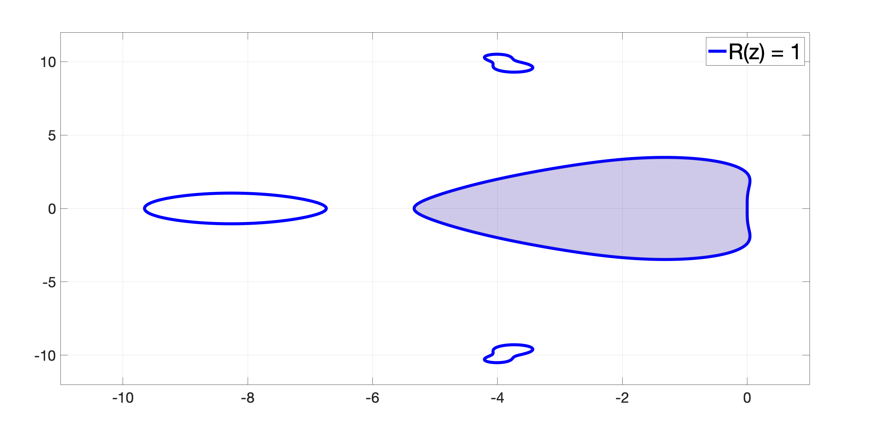
(a)

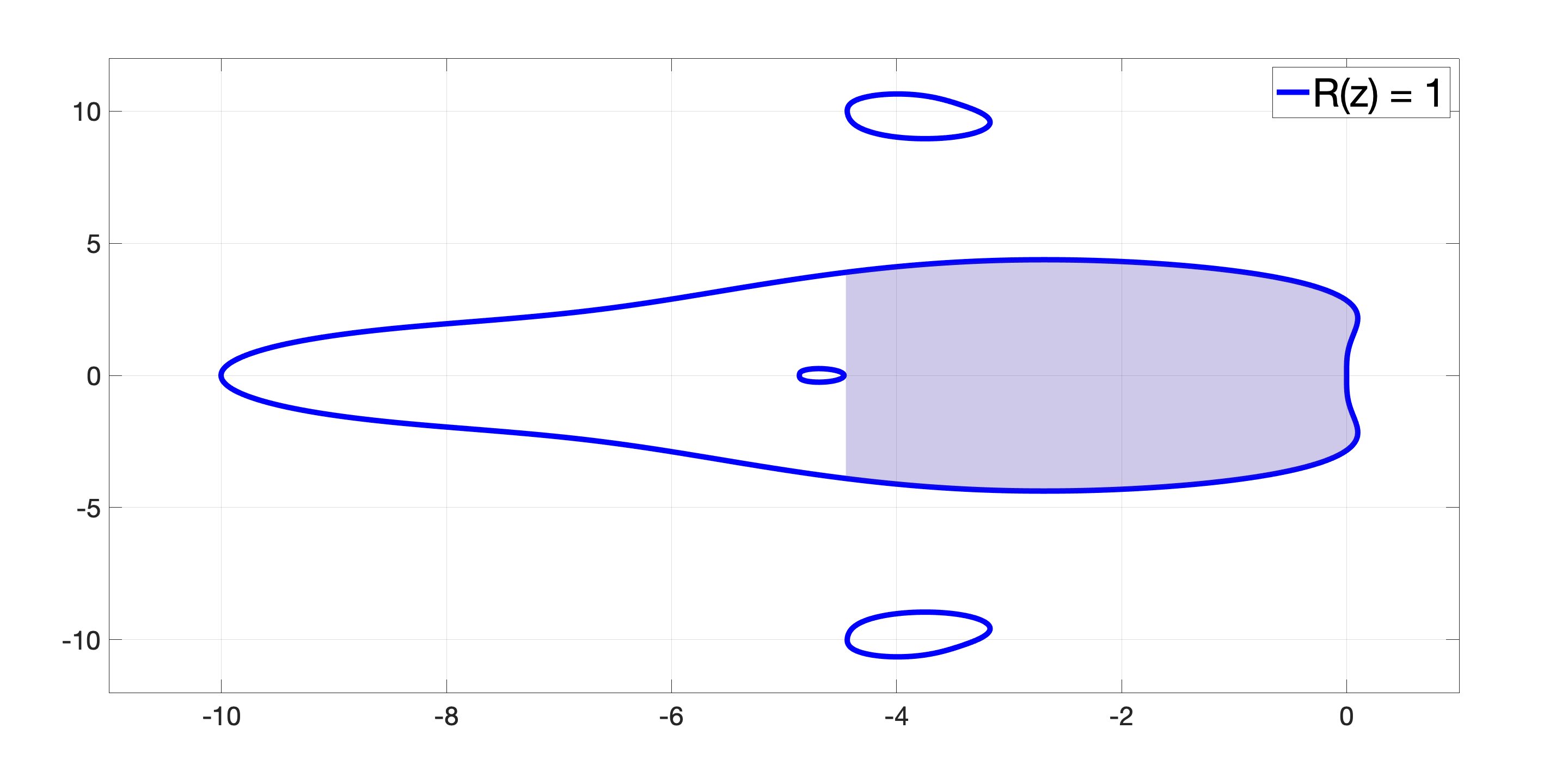
(b)

Figure 1: Examples of stability regions of FRSK methods that use one implicit and one explicit sub-integrator. Sub-regions relevant to stability of the method in practice when solving method-of-lines ODEs are shaded. Fig. 1(a): When a stability region consists of multiple disjointed parts, only the part that contains the origin is relevant to the stability of the method in practice. Fig. 1(b): If a hole of instability is present in the part of the stability region containing the origin, the right-most $x$-co-ordinate of the hole determines the largest stable step size in the presence of dominant negative real eigenvalues.

Theoretically, one can choose the sub-integration methods with full flexibility to optimize the stability region. For example, we often solve the stiff operator with an implicit method and the non-stiff operator with an explicit method. However, stability is not the only consideration when choosing a sub-integration method in practice; e.g., the computational cost of the non-linear solve may tip the balance in favor of an explicit sub-integration method. Therefore, for a given problem, we may choose the sub-integration method based on computational instead of stability considerations. We then focus on the choice of operator-splitting coefficients to improve the stability of the overall FSRK method.

Based on this analysis, we propose two strategies to mitigate the instability due to backward-in-time integration and at the same time reduce computational cost per step:

1. Choose operator-splitting coefficients and operator ordering so that the right-most negative $x$-intercept of $|R(z)|=1$ is located far from the origin. As noted by 2.1, changing the operator ordering is equivalent to solving the original operator ordering problem with the adjoint method.

2. Use an explicit Runge–Kutta method for backward-in-time sub-integrations. In this scenario, the idea is that an explicit Runge–Kutta method improves stability by removing the pole completely (because its stability function is a polynomial), and it also improves efficiency because explicit methods are generally less computationally expensive than implicit ones.

The effects of these strategies are demonstrated in Section 4.

3 Main results

In his 1968 paper [27], Strang mentioned three fundamental criteria when comparing numerical methods: accuracy, simplicity, and stability. In addition to the order of accuracy, we can characterize the accuracy of a method for a given order based on the local error measure [3]. Simplicity can be interpreted as the complexity of a method, or in this case, the number of sub-integrations required. Thus, it is associated with the computational cost of a method. The linear stability function can be used to characterize the stability of a fractional-step Runge–Kutta method [26]. In this section, we derive third-order operator-splitting methods by optimizing the linear stability region and local error measure. We include the simplicity (in the sense of computational cost) of the method in our analysis and discuss the effect of the operator ordering on the stability of the method. Accordingly, we minimize the LEM or $\hat{x}$ for a given number of stages while minimizing as well the number of sub-integrations. We denote an $N$-split operator-splitting method with $s$ stages, order $p$, and $f$ sub-integrations by OS${}_{N}(s,p)f$.

3.1 OS${}_{2}(4,3)7$ method with optimized LEM

To improve upon the LEM of the methods presented in Section 2.3 with minimal additional computational cost, we consider four-stage, third-order, 2-split methods with 7 sub-integrations; i.e., one of the coefficients $\{\alpha_{k}^{[\ell]}\}_{k=1,2,3,4}^{\ell=1,2}$ vanishes. Determination of such methods is performed as follows. For each $\alpha_{k}^{[\ell]}=0$, $k=1,2,3,4$, $\ell=1,2$, we minimize the LEM Eq. 11 using MATLAB’s GlobalSearch algorithm starting from 50 random seeds. From the candidate methods generated, we found two methods with the minimal LEM that are also adjoints of each other. We refer to one of these optimum methods as OS${}_{2}(4,3)7$${}_{\text{minLEM}}$. We note that there is no loss of generality through the choice made at this point because we have yet to specify operator ordering. The coefficients of OS${}_{2}(4,3)7$${}_{\text{minLEM}}$ are given to 15 decimal places in Table 3.

Table 3: Coefficients $\alpha_{k}^{[\ell]}$ of the OS${}_{2}(4,3)7$${}_{\text{minLEM}}$ method

$k$	$\displaystyle\alpha_{k}^{[1]}$	$\displaystyle\alpha_{k}^{[2]}$
1	$0.675603619637542$	$1.351207213243766$
2	$-0.175603577692365$	$-1.702414383919316$
3	$-0.175603614267295$	$1.351207170675550$
4	$0.675603572322118$	$0$

The required number of sub-integrations and the LEM (rounded to two decimal places) for Ruth, AKS3, and OS${}_{2}(4,3)7$${}_{\text{minLEM}}$ are given in Table 4. Although the OS${}_{2}(4,3)7$${}_{\text{minLEM}}$ method requires one more sub-integration than Ruth and AKS3, it may have better general accuracy properties given its comparatively small LEM. Hence, in principle, it may be able to overcome the added expense of an extra sub-integration per step by being able to take larger steps while maintaining the same accuracy and achieve improved performance. However, it turns out that the Niederer benchmark problem considered in Section 4 is too stability-constrained for this to be the case; see also Fig. 2 below.

Table 4: Summary of the properties of Ruth, AKS3, and OS${}_{2}(4,3)7$${}_{\text{minLEM}}$.

Method	$\#$ of sub-integrations	LEM
Ruth	$6$	$0.36$
AKS3	$6$	$0.25$
OS${}_{2}(4,3)7$${}_{\text{minLEM}}$	$7$	$6.55$110-8$$

3.2 Third-order, 2-split methods with optimized linear stability

As is shown in Section 2.4, given the most negative real eigenvalues $\lambda^{[D]}$ and $\lambda^{[R]}$ of each operator and the Runge–Kutta sub-integrators for each operator at each stage, the stability functions Eq. 13 or Eq. 14 of an FSRK method depends the operator-splitting coefficients $\displaystyle\{\alpha_{k}^{[\ell]}\}_{k=1,2,\dots,s}^{\ell=1,2}$. Fixing an operator ordering, we can achieve better stability, especially for problems with strictly real eigenvalues, by designing a method that minimizes $\hat{x}$, the right-most negative $x$-intercept of $|R(z)|=1$. When the Jacobians of the operators are simultaneously diagonalizable, this value is a good predictor of the largest stable step size in practice.We note that the adjoint of the optimal method can be used to solve the problem with the reversed operator ordering as indicated by 2.1.

Because we are interested in third-order operator-splitting methods with one implicit and one explicit sub-integrator, we use the two-stage, third-order SDIRK method with $\gamma=\displaystyle\frac{3+\sqrt{3}}{6}$ (SDIRK(2,3)) [13] and Kutta’s third-order explicit method (RK3) [17]. The stability functions of SDIRK(2,3) and RK3 are given by

$$R_{\text{SDIRK(2,3)}}(z) =1-\frac{z^{2}(2\gamma-1)}{2(\gamma z-1)^{2}}-\frac{z}{\gamma z-1},\quad\gamma=\frac{3+\sqrt{3}}{6},$$

$$R_{\text{RK3}}(z) =1+z+\frac{z^{2}}{2}+\frac{z^{3}}{6}.$$

The quantity $\hat{x}$ is minimized using the MATLAB GlobalSearch algorithm with $100$ random initial guesses for each case. We restrict the design space of each operator-splitting coefficient to the interval $[-1,1]$ because excessively large sub-steps are generally undesirable. Furthermore, backward sub-steps may be unstable, and accordingly, their lengths should generally be minimized. The operator-splitting method that gives the most negative $\hat{x}$ among the all candidates is then selected as the optimal method for the particular operator ordering.

In Section 4, we use the Niederer benchmark problem to explicitly demonstrate the performance of OS${}_{2}(3,3)6$ and OS${}_{2}(4,3)7$ methods with designed by optimizing linear stability and then further enhanced through judicious sub-integration.

4 Numerical experiments

The monodomain model is a popular mathematical model for cardiac electrophysiology [28]. It consists of a partial differential equation (PDE) that models the electrical activity in (co-located) intracellular and extracellular domains of myocardial tissue, coupled with a system of non-linear ODEs that describe the current density flowing through the membrane ionic channels. The monodomain model is a simplification of the bidomain model under the assumption that the intracellular conductivity is in constant proportion to the extracellular conductivity. Nonetheless, the monodomain model has practical utility along with its computational advantages [28]. Both the monodomain and bidomain models are computationally expensive because of the high resolution required from both spatial and temporal discretizations and the increasing size and complexity of the ionic membrane models. For these reasons, operator-splitting methods are used to achieve better efficiency and feasibility over monolithic approaches [28]. Software libraries for cardiac simulation typically implement the first-order Lie–Trotter method or the second-order Strang method for the simulation of the monodomain/bidomain models [28, 21, 8]. High-order methods have generally been considered unstable due to the backward-in-time integration. However, recent work has shown this is not necessarily the case [26], in particular for the monodomain and bidomain models [5, 6, 7]. In this section, we demonstrate various ways to improve the stability and efficiency of high-order operator-splitting methods to solve a well-known benchmark problem for the monodomain model.

A benchmark problem was studied in Niederer et al. [20] to verify and compare the performance of solutions of eleven myocardial tissue electrophysiology simulators. The benchmark problem consists of a 3D monodomain model described by the differential equations,

(15) $$\chi C_{m}\partialderivative{v}{t}+\chi{I_{\rm ion}}(\mathbf{s},v) =\nabla\cdot(\sigma\nabla v),$$

$$\partialderivative{\mathbf{s}}{t} =\mathbf{f}(t,\mathbf{s},v),$$

where $v$ is the transmembrane potential (or voltage), $\mathbf{s}$ is a set of variables describing the state of the cell, $\chi$ is the cell surface-to-volume ratio, $C_{m}$ is the specific membrane capacitance, and $\sigma$ is the conductivity tensor. The transmembrane current density, ${I_{\rm ion}}$, is defined by the cell model, whose states are governed by the ODEs with right-hand side $\mathbf{f}(t,\mathbf{s},v)$.

The Niederer benchmark problem is posed on a cuboid of dimension $0.3$ cm $\times\ 0.7$ cm $\times\ 2$ cm and time interval $[0,40]$ ms with a specified initial stimulus at a corner of the domain. The cell model used is that of ten Tusscher and Panfilov [29], a cell model of human epicardial myocytes. This cell model consists of 19 ODEs that model all the major ion channels and intracellular calcium dynamics. Details of the remaining parameters of the problem are given in [20]. To solve the Niederer benchmark problem numerically, we first discretize the 3D domain using central finite differences with a spatial mesh of size $\Delta x=\Delta y=\Delta z=0.05$ cm. A reference solution was computed by solving the problem with Strang splitting using the RK45 method in scipy.integrate.solve_ivp with rtol=1e-3 and atol=1e-6 as sub-integrators, and halving the time step until 3 digits matched across $4305$ equally spaced spatial points and $21$ temporal points $[0:2:40]$ ms.

To solve the Niederer benchmark problem using operator splitting, we split the resulting reaction-diffusion system into two operators, representing reaction and diffusion, respectively:

(16) $$\mathcal{F}^{[R]}=\left\{\begin{aligned} \partialderivative{v}{t}&=-\frac{1}{C_{m}}{I_{\rm ion}}(\mathbf{s},v),\\ \derivative{\mathbf{s}}{t}&=\mathbf{f}(t,\mathbf{s},v),\end{aligned}\right.\text{ and }\quad\mathcal{F}^{[D]}=\left\{\begin{aligned} \partialderivative{v}{t}&=\frac{1}{\chi C_{m}}\nabla\cdot(\sigma\nabla v),\\ \derivative{\mathbf{s}}{t}&=\mathbf{0}.\end{aligned}\right.$$

We solve the Niederer benchmark problem with different operator-splitting methods and different Runge–Kutta methods as sub-integrators. To measure the error of an FSRK method, we use the mixed root-mean-square (MRMS) error [19] of quantity $X$ [MRMS]_X at $M=4305\times 21$ space-time points defined by

$$[\text{MRMS}]_{X}=\sqrt{\frac{1}{M}\sum\limits_{i=1}^{M}\left(\frac{X_{i}-X_{i}^{\text{ref}}}{1+\absolutevalue{X_{i}^{\text{ref}}}}\right)^{2}},$$

where $X_{i}$ and $X_{i}^{\text{ref}}$, respectively, denote the numerical solution and the reference solution. Because the transmembrane potential $v$ is the main variable of interest, we focus on [MRMS]_v for the analysis. In practice, we set a level $[\text{MRMS}]_{v}=0.05$ as an acceptable error threshold. To examine the efficiency of these methods, we find the largest constant step sizes $\Delta t$ to two significant figures that yields [MRMS]${}_{v}\leq 0.05$. These step sizes are then used to solve the Niederer benchmark problem over the interval $[0,40]$. The simulations were performed using the pythOS operator splitting library [11] on an HP Z820 workstation running 64-bit Ubuntu 20.04 LTS with Linux kernel 5.4.0-177-generic. The machine has an Intel Xeon E5-2650 2.0 GHz octa-core CPU and 512 GB of 1600 MHz DDR3 RAM. CPU times using are reported as the minimum of three runs after checking for consistency.

For the Niederer benchmark problem, the most negative eigenvalues of the Jacobians of the diffusion and reaction operators are $\lambda^{[D]}\approx-1.92$ and $\lambda^{[R]}=-1260$ [24], respectively. For a given FSRK method, we form stability functions $R_{DR}(z)$, where the first operator is the diffusion operation and the second operator is the reaction operator, and $R_{RD}(z)$, where the first operator is the reaction operation and the second operator is the diffusion operator, as given in Eq. 13.

4.1 Optimized LEM

The stability regions of OS${}_{2}(4,3)7$${}_{\text{minLEM}}$ for the DR and RD orderings are shown in Fig. 2. Comparing Figs. 2 and 3, we see that the stability regions for both DR and RD orderings of OS${}_{2}(4,3)7$${}_{\text{minLEM}}$ are comparable to AKS3 but significantly smaller than those with optimized $\hat{x}$. These results suggest that OS${}_{2}(4,3)7$${}_{\text{minLEM}}$ would underperform OS${}_{2}(4,3)7$${}_{DR\hat{x}}$ derived in Section 4.2. Indeed, numerical experiments confirm that optimizing LEM does not lead to better performance for this example. Hence, we do not report on the OS${}_{2}(4,3)7$${}_{\text{minLEM}}$ method further.

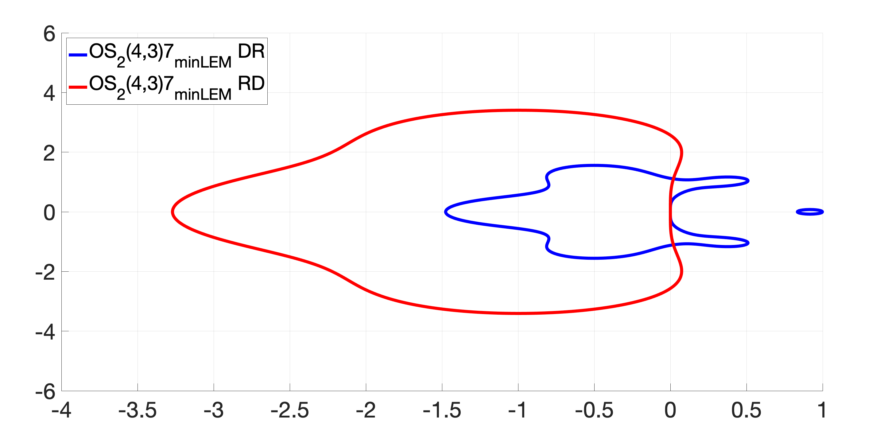
Figure 2: Stability regions of the OS${}_{2}(4,3)7$${}_{\text{minLEM}}$ method applied to the Niederer benchmark problem with different operator orderings.

4.2 Optimized linear stability

For the case of OS${}_{2}(3,3)6$ methods, we find the best result is a method whose $\hat{x}$ is marginally more negative than that of the Ruth method, which implies that it will allow a slightly larger step-size than that allowed by the Ruth method. However, because the computational cost per step for this method is the same as the Ruth method, it is not expected this method will achieve a significant improvement in the overall efficiency. Hence, the class of OS${}_{2}(3,3)6$ methods is not considered further.

For the class of OS${}_{2}(4,3)7$ methods, the coefficients of the best method in the DR ordering are given to 15 decimal places in Table 5. We denote this method by OS${}_{2}(4,3)7$${}_{DR\hat{x}}$. The best method with the RD ordering is the adjoint of OS${}_{2}(4,3)7$${}_{DR\hat{x}}$.

Table 5: Coefficients $\alpha_{k}^{[\ell]}$ for the OS${}_{2}(4,3)7$${}_{DR\hat{x}}$ method.

$k$	$\displaystyle\alpha_{k}^{[1]}$	$\displaystyle\alpha_{k}^{[2]}$
1	$0$	$0.214870149852186$
2	$0.511486052225367$	$0.668690687888393$
3	$-0.501427388979812$	$-0.041956908041494$
4	$0.989941336754445$	$0.158396070300915$

4.3 Operator ordering for optimal stability

As discussed in Section 2.4, the order of the operators should be chosen that the right-most negative $x$-intercept of $|R(z)|=1$ is far from the origin. In Fig. 3, we compare the stability regions of the Ruth, AKS3, and OS${}_{2}(4,3)7$${}_{DR\hat{x}}$ methods applied to the Niederer benchmark problem with different operator orderings: diffusion-reaction (DR) and reaction-diffusion (RD). The interior regions correspond to $|R(z)|<1$. The stability plots show that when using the Ruth method, the RD ordering is more stable, and when using the OS${}_{2}(4,3)7$${}_{DR\hat{x}}$ method, the DR ordering is more stable. These orderings suggest that it is preferable to integrate the stiff reaction operator backward for as short an interval as possible.

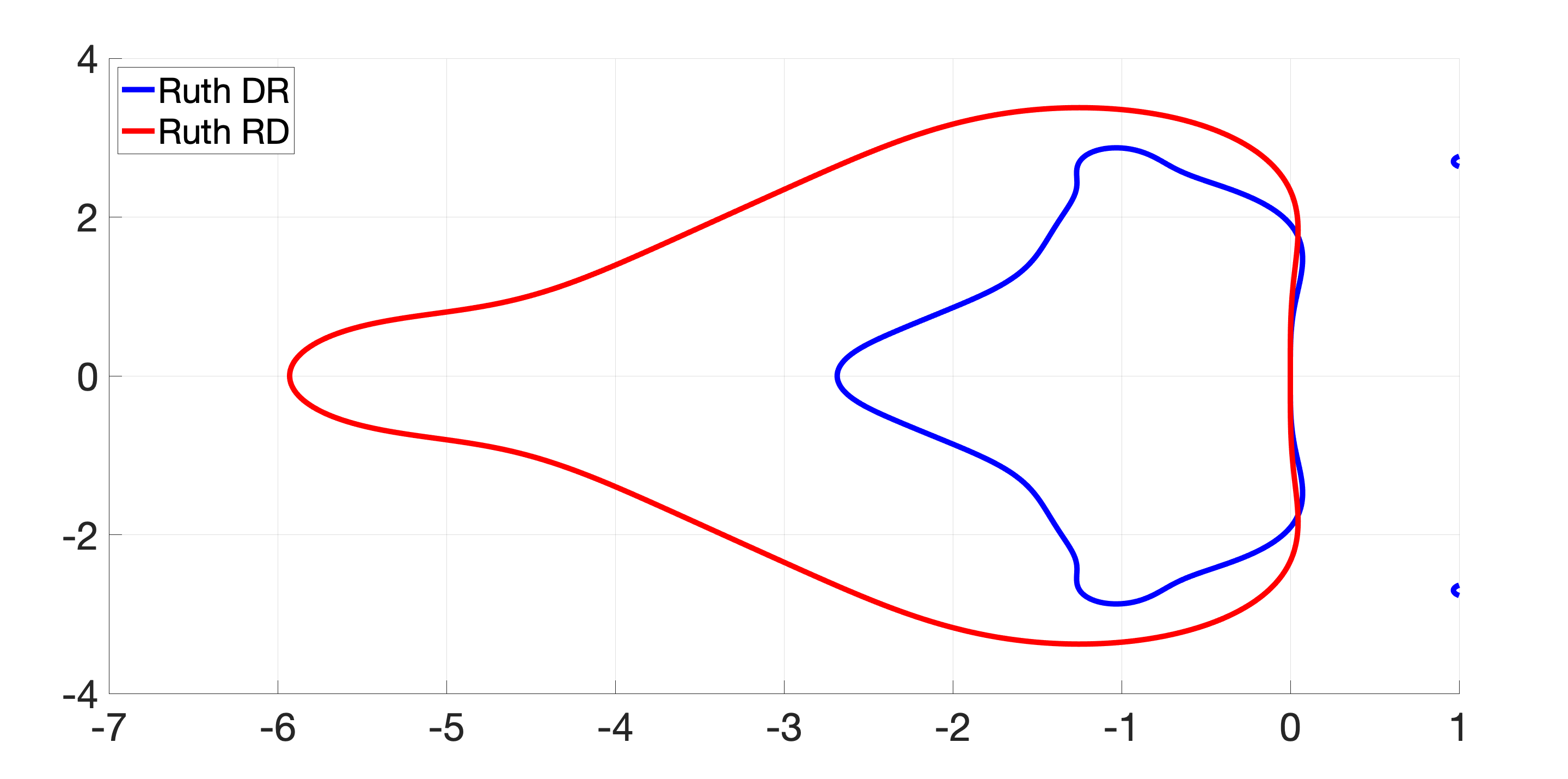
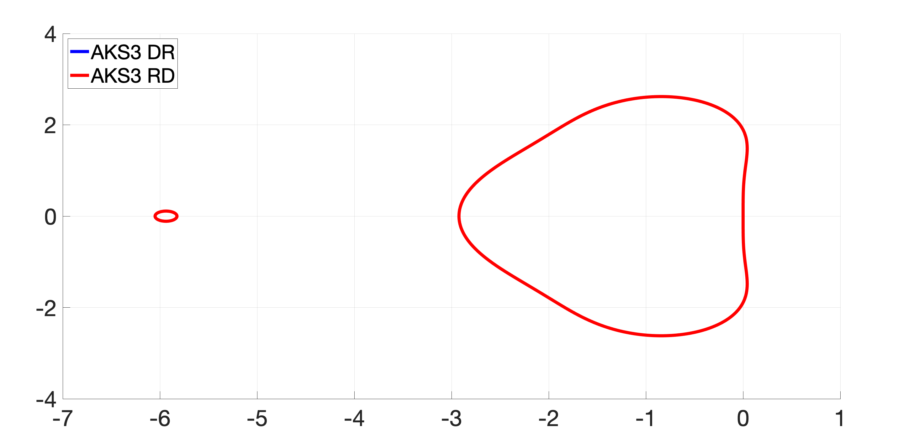
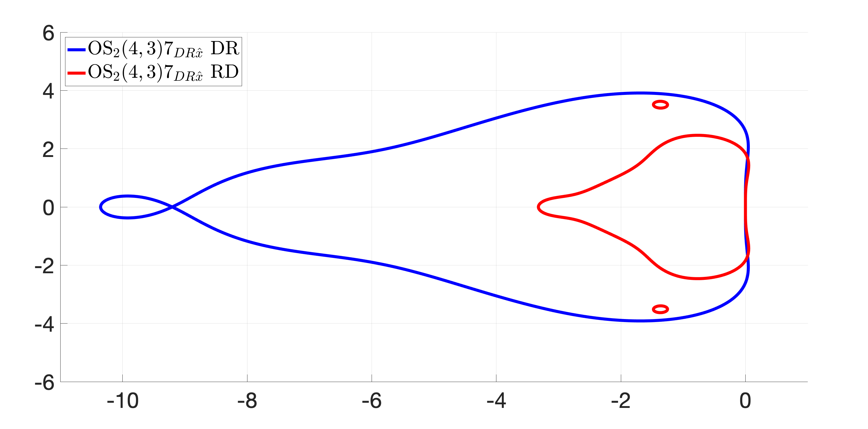
Figure 3: Stability regions of the Ruth, AKS3, and OS${}_{2}(4,3)7$${}_{DR\hat{x}}$ methods applied to the Niederer benchmark problem with different operator orderings.

We note that, in this case, no hole of instability appears in the main stability region; therefore, the stability of the methods is not dictated by the location of the pole on the left-hand side of the complex plane. If the stability region is restricted by a hole as in Fig. 1(b), the operator ordering that places the pole further to the left normally improves the stability property [26].

4.4 Performance of OS${}_{2}(4,3)7$ methods

The CPU times using the Ruth, AKS3, and OS${}_{2}(4,3)7$${}_{DR\hat{x}}$ methods are reported in Table 6. The results confirm the optimal integration orderings suggested in Fig. 3, i.e., the Ruth method can take a larger stable step size with operator ordering RD and OS${}_{2}(4,3)7$${}_{DR\hat{x}}$ can take a larger stable step size with operator ordering DR. We note that this computation is stability constrained because the [MRMS]_v errors for the allowed step sizes are well below $0.05$. The OS${}_{2}(4,3)7$${}_{DR\hat{x}}$ method exhibit a $36\%$ efficiency gain compared to the Ruth method (in RD order). AKS3 is less stable than the Ruth method for this problem, and so the advantage of a smaller LEM does not lead to a practical advantage for this (stability-constrained) problem.

Remark 4.1.

Fig. 3 suggests that the OS${}_{2}(4,3)7$${}_{DR\hat{x}}$ method applied in the RD ordering, i.e., in the opposite ordering for which it was designed, has a much smaller stable step size compared to the Ruth method. In other words, this new method is inefficient when not used according to its design principles. Accordingly, we omit details of this combination in Table 6.

method	Diffusion-Reaction			Reaction-Diffusion
	$\Delta t$	time	MRMS error	$\Delta t$	time	MRMS error
Ruth	0.0028	8831	0.00067	0.0062	3962	0.00039
AKS3	0.0031	7654	0.023	0.0031	7969	0.022
OS${}_{2}(4,3)7$${}_{DR\hat{x}}$	0.011	2509	0.00055	—	—	—

Table 6: Efficiency comparison of solving the Niederer benchmark problem using the Ruth, AKS3, and OS${}_{2}(4,3)7$${}_{DR\hat{x}}$ methods.

.

4.5 Use of explicit Runge–Kutta methods for backward-in-time integration

A further way to improve the linear stability of a fractional-step Runge–Kutta method is to remove any poles in the linear stability region in the left-hand side of the complex plane. Such poles can be caused by backward-in-time sub-integration with an implicit Runge–Kutta method. In such cases, the pole can be removed by replacing an implicit Runge–Kutta sub-integrator with an explicit Runge–Kutta sub-integrator when integrating backward in time. Because the Niederer benchmark problem is stability constrained and not accuracy constrained for the parameters chosen, we replace the negative steps in both operators with the forward Euler (FE) method. Interestingly, when integrating backward in time, the FE method in fact leads to a method with a larger linear stability region than Heun’s method, which is in turn more stable than Kutta’s third-order method, because, for $z$ values with positive real parts, $|R_{\text{FE}}(z)|<|R_{\text{Heun}}(z)|<|R_{\text{RK3}}(z)|$. Moreover, although use of the FE method negatively impacts the order of the overall method (and generally the accuracy of a given numerical solution), it has the least computational expense per step, and so the increase in error does not negate the increase in efficiency in this situation.

As shown in Figs. 4 and 5, replacing both SDIRK(2,3) and RK3 with FE for the negative steps made slight improvement in stability of all the Ruth, AKS3, OS${}_{2}(4,3)7$${}_{DR\hat{x}}$ methods.

As shown in Table 7, although the use of the forward Euler method increased the error in each computation, all errors are still acceptable. All methods, moreover, demonstrate significant efficiency gains. Although the improvement in stability leads to no further improvement in step size in this case, the OS${}_{2}(4,3)7$${}_{DR\hat{x}}$ method is approximately $25\%$ faster than the classical implementation reported in Table 6 and $29\%$ faster than the optimal implementation of the Ruth method.

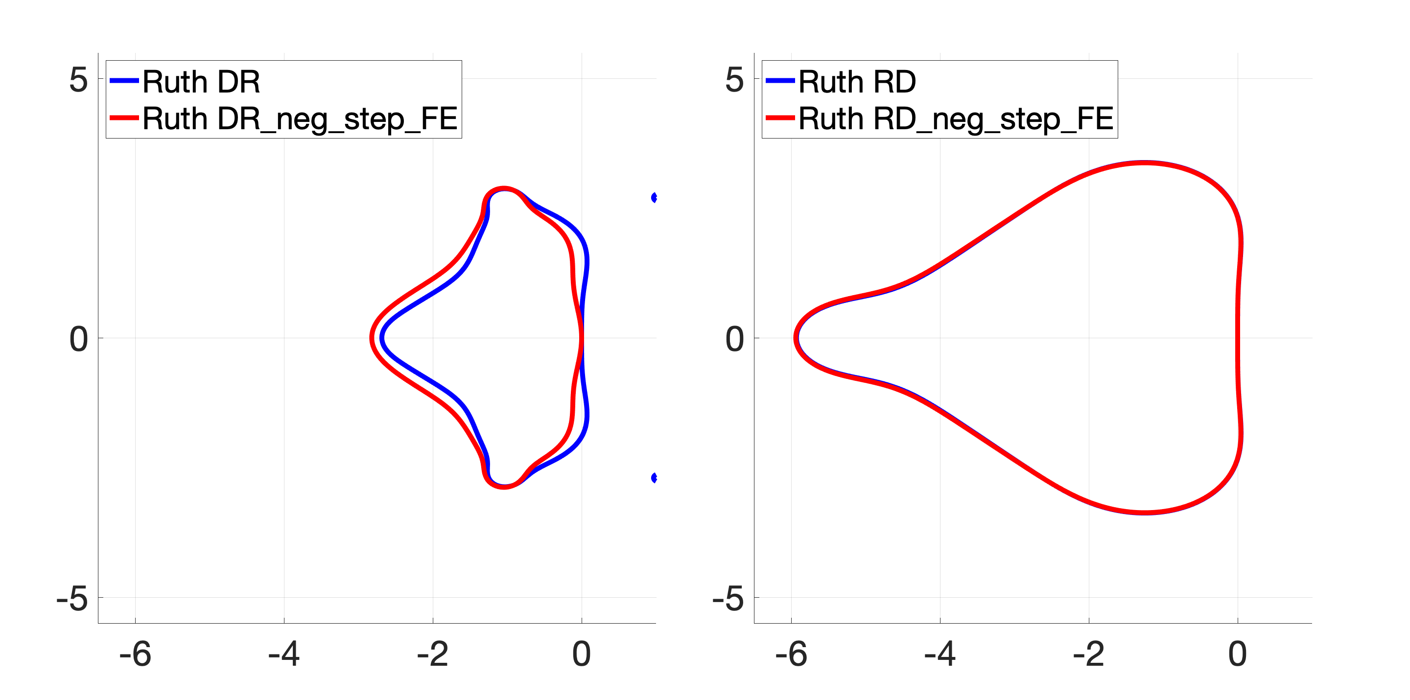
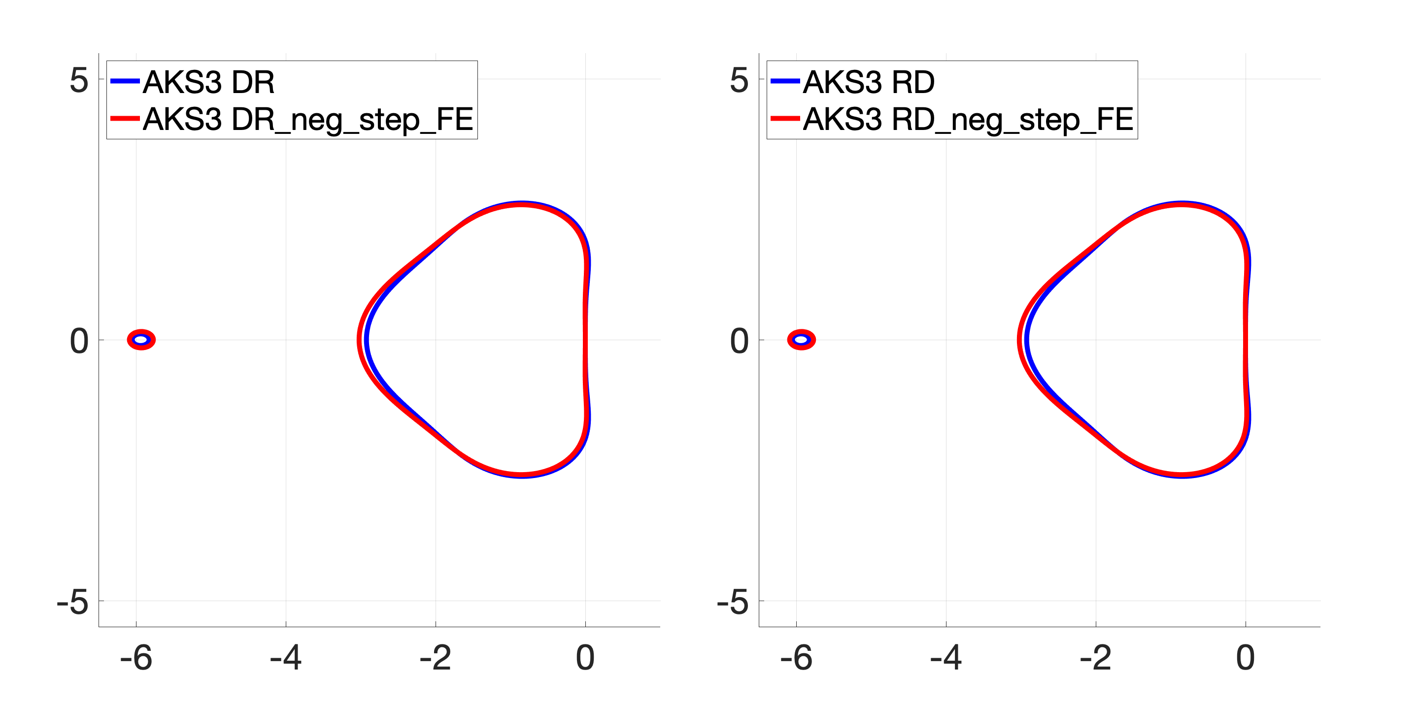
Figure 4: Stability regions of the Ruth and AKS3 applied to the Niederer benchmark problem with different operator orderings and FE applied to both negative steps.

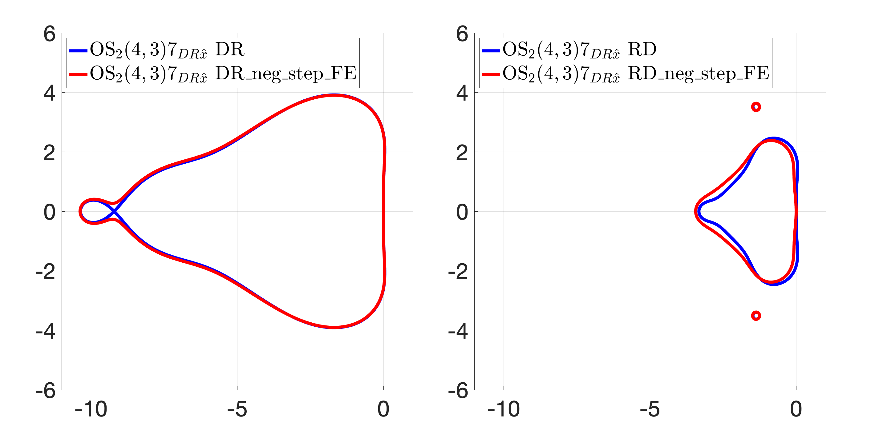
Figure 5: Stability regions of the OS${}_{2}(4,3)7$${}_{DR\hat{x}}$ applied to the Niederer benchmark problem with different operator orderings and FE applied to both negative sub-integrations.

method	DR (FE for both neg)			RD (FE for both neg)
	$\Delta t$	time	error	$\Delta t$	time	error
Ruth	0.0029	5752	0.021	0.0062	2678	0.041
AKS3	0.0031	5338	0.024	0.0031	5290	0.024
OS${}_{2}(4,3)7$${}_{DR\hat{x}}$	0.011	1906	0.0414	—	—	—

Table 7: Efficiency comparison of solving the Niederer benchmark problem using the Ruth, AKS3, and OS${}_{2}(4,3)7$${}_{DR\hat{x}}$ methods with the DR and RD orderings using forward Euler for both backward-in-time sub-integrations.

5 Conclusions

In this paper, we constructed a new four-stage, third-order, 2-split operator-splitting method with seven sub-integrations per time step and improved linear stability and computational efficiency over existing methods and implementations. The method was designed by optimizing the linear stability region on the negative real axis while considering the number and type of sub-integrations. This optimization represents balancing the tradeoff of stability against computational expense per step. Moreover, we also proposed two novel implementation strategies to improve the stability of FSRK methods for a given problem. First, operator ordering can be chosen to optimize the stability. Second, replacing an implicit Runge–Kutta sub-integrator with an explicit Runge–Kutta sub-integrator for backward-in-time sub-integrations generally improves efficiency and can yield (sometimes substantial) increases in stability. When low-order explicit Runge–Kutta sub-integrators are used, the increase in efficiency may nonetheless offset the increase in error, especially for stability-constrained problems. For future work, we plan to further explore high-order operator-splitting methods with an emphasis on problems where the Jacobians are not simultaneously diagonalizable.

References

- [1] U. M. Ascher, S. J. Ruuth, and R. J. Spiteri, Implicit-explicit Runge–Kutta Methods for Time-dependent Partial Differential Equations, Applied Numerical Mathematics, 25 (1997), pp. 151–167.
- [2] W. Auzinger and W. Herfort, Local error structures and order conditions in terms of Lie elements for exponential splitting schemes, Opuscula Mathematica, 34 (2014), pp. 243–255.
- [3] W. Auzinger, H. Hofstätter, D. Ketcheson, and O. Koch, Practical splitting methods for the adaptive integration of nonlinear evolution equations. Part I: Construction of optimized schemes and pairs of schemes, BIT Numerical Mathematics, 57 (2017), pp. 55–74.
- [4] S. Blanes, F. Casas, and A. Murua, Splitting methods for differential equations, arXiv.org, (2024).
- [5] J. Cervi and R. J. Spiteri, High-order operator splitting for the bidomain and monodomain models, SIAM Journal on Scientific Computing, 40 (2018), pp. A769–A786.
- [6] J. Cervi and R. J. Spiteri, High-order operator-splitting methods for the bidomain and monodomain models, in Mathematical and Numerical Modeling of the Cardiovascular System and Applications, Springer, 2018, pp. 23–40.
- [7] J. Cervi and R. J. Spiteri, A comparison of fourth-order operator splitting methods for cardiac simulations, Applied Numerical Mathematics, 145 (2019), pp. 227–235.
- [8] J. Cooper, R. J. Spiteri, and G. R. Mirams, Cellular cardiac electrophysiology modeling with chaste and cellml, Frontiers in physiology, 5 (2015), pp. 511–511.
- [9] S. K. Godunov, A difference method for numerical calculation of discontinuous solutions of the equations of hydrodynamics, Matematicheskii Sbornik, 89 (1959), pp. 271–306.
- [10] G. Goldman and T. J. Kaper, Nth-order operator splitting schemes and nonreversible systems, SIAM Journal on Numerical Analysis, 33 (1996), pp. 349–367.
- [11] V. Guenter, S. Wei, and R. J. Spiteri, pythos: A Python library for solving IVPs by operator splitting, https://arxiv.org/abs/2407.05475, https://arxiv.org/abs/https://arxiv.org/abs/2407.05475.
- [12] E. Hairer, C. Lubich, and G. Wanner, Geometric numerical integration: structure-preserving algorithms for ordinary differential equations, vol. 31, Springer Science & Business Media, 2006.
- [13] E. Hairer, S. P. Nørsett, and G. Wanner, Solving ordinary differential equations. I, vol. 8 of Springer Series in Computational Mathematics, Springer-Verlag, Berlin, second ed., 1993. Nonstiff problems.
- [14] E. Hansen and A. Ostermann, High order splitting methods for analytic semigroups exist, BIT, 49 (2009), pp. 527–542.
- [15] C. A. Kennedy and M. H. Carpenter, Additive Runge–Kutta schemes for convection–diffusion–reaction equations, Applied Numerical Mathematics, 44 (2003), pp. 139–181.
- [16] D. I. Ketcheson and H. Ranocha, Computing with b-series, ACM transactions on mathematical software, 49 (2023), pp. 1–23.
- [17] W. Kutta, Beitrag zur naherungsweisen integration totaler differentialgleichungen, Z. Math. Phys., 46 (1901), pp. 435–453.
- [18] G. I. Marchuk, On the theory of the splitting-up method., in Numerical Solution of Partial Differential Equations-II, Academic Press, 1971, pp. 469 – 500.
- [19] M. E. Marsh, S. Ziaratgahi, and R. J. Spiteri, The Secrets to the Success of the Rush–Larsen Method and its Generalizations, IEEE Transactions on Biomedical Engineering, 59 (2012), pp. 2506–2515.
- [20] S. A. Niederer, E. Kerfoot, A. P. Benson, M. O. Bernabeu, O. Bernus, C. Bradley, E. M. Cherry, R. Clayton, F. H. Fenton, A. Gary, et al., Verification of cardiac tissue electrophysiology simulators using an N-version benchmark, Philosophical Transactions of the Royal Society A, 369 (2011), pp. 4331–4351.
- [21] G. Plank, A. Loewe, A. Neic, C. Augustin, Y.-L. Huang, M. A. Gsell, E. Karabelas, M. Nothstein, A. J. Prassl, J. Sánchez, G. Seemann, and E. J. Vigmond, The opencarp simulation environment for cardiac electrophysiology, Computer Methods and Programs in Biomedicine, 208 (2021), p. 106223, https://doi.org/https://doi.org/10.1016/j.cmpb.2021.106223, https://www.sciencedirect.com/science/article/pii/S0169260721002972.
- [22] R. D. Ruth, A canonical integration technique, IEEE Transactions on Nuclear Science, 30 (1983), pp. 2669–2671.
- [23] A. Sandu and M. Günther, A generalized-structure approach to additive Runge–Kutta methods, SIAM Journal on Numerical Analysis, 53 (2015), pp. 17–42.
- [24] R. J. Spiteri and R. C. Dean, Stiffness analysis of cardiac electrophysiological models, Annals of Biomedical Engineering, 38 (2010), pp. 3592–3604.
- [25] R. J. Spiteri, A. Tavassoli, S. Wei, and A. Smolyakov, Practical 3-splitting beyond Strang, 2023, https://arxiv.org/abs/2302.08034.
- [26] R. J. Spiteri and S. Wei, Fractional-step Runge–Kutta methods: Representation and linear stability analysis, Journal of computational physics, 476 (2023), p. 111900.
- [27] G. Strang, On the construction and comparison of difference schemes, SIAM Journal on Numerical Analysis, 5 (1968), pp. 506–517.
- [28] J. Sundnes, G. T. Lines, and X. Cai, Computing the Electrical Activity in the Heart, Springer, 2006.
- [29] K. H. ten Tusscher and A. V. Panfilov, Alternans and spiral breakup in a human ventricular tissue model, American Journal of Physiology - Heart and Circulatory Physiology, 291 (2006), pp. H1088–H1100.
- [30] H. F. Trotter, Approximation of semi-groups of operators., Pacific Journal of Mathematics, 8 (1958), pp. 887–919.
- [31] R. Tyson, L. G. Stern, and R. J. LeVeque, Fractional step methods applied to a chemotaxis model, J. Math. Biol., 41 (2000), pp. 455–475, https://doi.org/10.1007/s002850000038.
- [32] S. Wei and R. J. Spiteri, Qualitative property preservation of high-order operator splitting for the sir model, Applied Numerical Mathematics, 172 (2022), pp. 332–350.
- [33] N. N. Yanenko, The method of fractional steps. The solution of problems of mathematical physics in several variables, Springer-Verlag, New York-Heidelberg, 1971. Translated from the Russian by T. Cheron. English translation edited by M. Holt.
- [34] H. Yoshida, Construction of higher order symplectic integrators, Physics Letters A, 150 (1990), pp. 262–268.