Detecting high-dimensional entanglement by local randomized projections

Abstract

The characterization of high-dimensional entanglement plays a crucial role in the field of quantum information science. Conventional methods perform either fixed measurement bases or randomized measurements with high-order moments. Here, we introduce a criterion for estimating the Schmidt number of bipartite high-dimensional states based on local randomized projections with first-order moments. To extract more information from limited experimental data, we propose an estimation algorithm of the Schmidt number. We exhibit the performance of the proposed approach by considering the maximally entangled state under depolarizing and random noise models. Our approach not only obtains a more accurate estimation of the Schmidt number but also reduces the number of projections compared to known methods.

Introduction—Quantum entanglement is a valuable resource in various quantum applications from quantum cryptography [1, 2, 3], quantum metrology [4, 5, 6], and quantum computation [7, 8]. The preparation, manipulation, and characterization of quantum entanglement are important in quantum information science. Beyond qubit systems, high-dimensional entanglement has attracted tremendous interest from bipartite [9, 10, 11, 12, 13, 14] to multipartite systems [15, 16]. The preparation of high-dimensional entangled states is feasible in different experimental platforms such as polar molecules [17], cold atomic ensembles [18], trapped ions [19], and photonic systems [20, 21, 22, 23]. High-dimensional entanglement in quantum communication brings several benefits by increasing information capacity [24] and improving noise resistance [25, 9, 26]. These advantages have sparked significant interest in the characterization of high-dimensional entanglement.

Entanglement witness provides an experimentally feasible way to detect entanglement of high-dimensional states [27, 28]. The typical Schmidt number $(\mathrm{SN})$ witness is defined by the fidelity between the target state and a maximally entangled pure state $|\phi_{d}^{+}\rangle=\frac{1}{\sqrt{d}}\sum_{j=1}^{d}|jj\rangle$. Nevertheless, the direct measurement of the fidelity-based SN witness has become increasingly challenging as the dimension grows, mainly due to the requirement of $d(d+1)$ projections [29]. To reduce the experimental cost, alternative methods have been proposed by measuring the correlations in fixed measurement bases such as mutually unbiased bases (MUBs) [30, 31, 30, 32, 33]. According to the number of employed MUBs, a sequence of $\mathrm{SN}$ criteria has been introduced [34]. This strategy is quite powerful in verifying high $\mathrm{SN}$ with a small number of measurements.

More recently, randomized measurements (RMs) have been introduced to analyze entanglement [35, 36, 37, 38, 39]. In particular, one rotates a bipartite state by random local unitary and then measures the local observables. Using the measured second- and fourth-order moments, one infers the $\mathrm{SN}$ by a classical optimization [40, 41]. RMs allow the experimenter to measure the state on a random measurement basis and are thus suitable for different experimental platforms.

However, both methods above still face limitations. One limitation is the trade-off between the accuracy of estimating the $\mathrm{SN}$ and the number of implemented MUBs [34]. While measuring a small number of projections experimentally is required, one obtains a less precise lower bound on the $\mathrm{SN}$. To improve accuracy, constructing and measuring more sets of MUBs is necessary, which poses significant challenges [31, 30, 32, 42]. Other randomized-based methods often encounter a large number of experimental runs and high-order unitary designs due to their reliance on high-order moments [40, 41]. For instance, verifying a $5\otimes 5$ bipartite state requires $800$ random unitaries [43]. These challenges emphasize the need for experimentally feasible and powerful strategies to analyze bipartite high-dimensional entanglement.

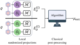
Figure 1: Illustration of our approach for estimating the Schmidt number of a bipartite high-dimensional state $\varrho$. The process consists of local randomized projections (LRPs) and classical post-processing. Both parties sample $N$ random unitaries $\{U_{l}\}_{l=1}^{N}$ and $N$ random orthogonal transformations $\{O_{l}\}_{l=1}^{N}$ independently from the Haar measure on unitary and orthogonal groups [44, 45, 46, 47]. LRPs implement local operations $U_{l}\otimes U_{l}$ and $O_{l}\otimes O_{l}$ and then measure on well-constructed observables $\mathcal{M}$ and $\hat{\mathcal{M}}$. From the obtained expectation values $E_{U}^{l}$ and $E_{O}^{(l)}$, the algorithm outputs the Schmidt number estimation $\mu_{\mathrm{est}}$.

In this work, we address the above issues and detect the entanglement of a bipartite high-dimensional state using local randomized projections. The overall procedure is shown in Fig. 1. In particular, Alice and Bob rotate the state locally under the same unitary or orthogonal transformation, followed by measurements on local observables. By analyzing the obtained first-order moments, we propose a criterion to estimate the Schmidt number of a target state, which approaches the fidelity-based witness [48, 49] with increasing number of random operations. Practically, we introduce an estimated algorithm to extract more information from the measured experimental data with limited local projections. This algorithm enables us to assess a lower bound of the Schmidt number. We apply our approach to mixed states with dimensions $d=20,30$. The numerical results indicate that $12$ random unitaries and $12$ random orthogonal transformations are sufficient to obtain a better estimation of the Schmidt numbers than previous approaches based on MUBs [34] and second-order moments in randomized measurements [40, 41]. The number of projections in our approach is independent of dimensions, while the number of projections increases linearly with the dimensions when using MUBs [34]. Thus, our approach significantly reduces the resource costs for analyzing the entanglement of bipartite high-dimensional states.

Schmidt number and fidelity-based witness.—The Schmidt number ($\mathrm{SN}$) of a pure quantum state $|\psi\rangle$ is defined by Schmidt rank ($\mathrm{SR}$), i.e., the number of nonzero Schmidt coefficients in their Schmidt decomposition [50], $|\psi\rangle=\sum_{j=1}^{\mu}\sqrt{s_{j}}|a_{j}b_{j}\rangle$, where $s_{j}>0$, $\sum_{j}s_{j}=1$, $\mu$ denotes the $\mathrm{SR}$, and $\{a_{j}\}$, $\{b_{j}\}$ are respectively orthonormal states. For mixed state $\varrho$, its $\mathrm{SN}$ is defined by [50], $\mathrm{SN}(\varrho)=\min_{\mathcal{D}(\varrho)}\{\mu_{\max}:\varrho=\sum_{j}p_{j}|\psi_{j}\rangle\langle\psi_{j}|,\mu_{\max}=\max_{j}\mu_{j}\}$, where $\mu_{j}$ is the $\mathrm{SR}$ of pure state $|\psi_{j}\rangle$ and $\mathcal{D}(\varrho)$ denotes the set of all pure-state decomposition of the state $\varrho$. The $\mathrm{SN}(\varrho)$ is an integer $[1,d]$. A larger $\mathrm{SN}$ in a bipartite state implies a higher degree of entanglement.

A typical way to determine the $\mathrm{SN}$ of a state $\varrho$ is to estimate the fidelity $F(\varrho)={\mathrm{tr}}(\varrho|\phi_{d}^{+}\rangle\langle\phi_{d}^{+}|)$ between $\varrho$ and a maximally entangled state $|\phi_{d}^{+}\rangle=\sum_{j=1}^{d}|jj\rangle/\sqrt{d}$. For any $\varrho$ with $\mathrm{SN}(\varrho)=\mu$, $F(\varrho)\leq\mu/d$ [50]. This inequality can be transformed into an $\mathrm{SN}=\mu+1$ witness, $\mathcal{W}_{\mu}=\mu\mathbbm{1}_{d}^{\otimes 2}/d-|\phi_{d}^{+}\rangle\langle\phi_{d}^{+}|$ [50, 48, 49, 51] such that ${\mathrm{tr}}(\varrho\mathcal{W}_{\mu})\geq 0$ for all $\varrho$ with $\mathrm{SN}(\varrho)\leq\mu$, where $\mathbbm{1}_{d}$ denotes the identity. Thus, if ${\mathrm{tr}}(\varrho\mathcal{W}_{\mu})<0$, $\varrho$ has at least $\mathrm{SN}(\varrho)=\mu+1$.

Schmidt number criterion via local randomized projections.—Consider a two-qudit state $\varrho$ shared by Alice and Bob. To detect the $\mathrm{SN}$ of $\varrho$, we measure $\varrho$ with local randomized projections. The measurement process includes two stages. The first stage allows Alice and Bob to perform measurements with any local observables $\mathcal{M}\otimes\mathcal{M}$ after applying the same random unitary $U\otimes U$ on the state $\varrho$. The expectation values for a fixed unitary $U$ is, $E_{U}(\varrho)={\mathrm{tr}}[\varrho(U\otimes U)(\mathcal{M}\otimes\mathcal{M})(U^{{\dagger}}\otimes U^{{\dagger}})]$. This randomized measurement strategy has been used to analyze multiparticle entanglement [38] and classify topological order [52]. When Alice and Bob are on the same platform, the joint operation $U\otimes U$ can be implemented by passing both parties through a single $U$ setup at different times, thereby reducing the operational costs while simultaneously mitigating imperfections of the unitary.

The second stage uses instead a random orthogonal transformation $O$, $O^{\top}O=OO^{\top}=\mathbbm{1}_{d}$, where $\top$ denotes the transpose operation. In this scenario, Alice and Bob implement the same orthogonal transformation $O\otimes O$ on the state $\varrho$ and perform measurements with local observables $\hat{\mathcal{M}}\otimes\hat{\mathcal{M}}$. The well-constructed observable satisfies $\hat{\mathcal{M}}=-\hat{\mathcal{M}}^{\top}$. The expectation value for a fixed orthogonal transformation $O$ is, $E_{O}(\varrho)={\mathrm{tr}}[\varrho(O\otimes O)(\hat{\mathcal{M}}\otimes\hat{\mathcal{M}})(O^{\top}\otimes O^{\top})]$. The implementation of $O\otimes O$ can also be simplified using a strategy similar to that of $U\otimes U$.

After sampling random unitary $U$ and orthogonal transformation $O$ respectively according to the Haar measure on unitary and orthogonal groups [44, 45, 46, 47], we consider two first-order moments,

$$\mathcal{R}(\varrho)\!=\!\int\!dUE_{U}(\varrho),\leavevmode\nobreak\ \mathcal{Q}(\varrho)\!=\!\int\!dOE_{O}(\varrho).$$ (1)

We adopt the optimal observables with the smallest rank, given by $\mathcal{M}=|j\rangle\langle j|$ and $\hat{\mathcal{M}}=-i|1\rangle\langle d|+i|d\rangle\langle 1|$, where $\{|j\rangle\}_{j=1}^{d}$ denotes the computational bases in a $d$-dimension Hilbert space and $i=\sqrt{-1}$. We have then, see Appendix A,

$$\mathcal{R}(\varrho) =\frac{1+{\mathrm{tr}}(\varrho\mathbb{S})}{d(d+1)},\mathcal{Q}(\varrho)=\frac{2{\mathrm{tr}}\left[\varrho\left(\mathbb{S}-\mathbb{S}^{\top_{B}}\right)\right]}{d(d-1)},$$ (2)

by using the Schur–Weyl duality in the unitary and orthogonal group [44, 45, 46, 47, 53, 54, 55, 56]. Here, $\mathbb{S}=\sum_{j,k=1}^{d}|jk\rangle\langle kj|$ is the $\mathrm{SWAP}$ operator and $\top_{B}$ denotes the partial transpose to the subsystem B.

Now, we present our result showing that the moments $\mathcal{R}(\varrho)$ and $\mathcal{Q}(\varrho)$ in Eq. (2) can be used to calculate the fidelity $F(\varrho)={\mathrm{tr}}(\varrho|\phi_{d}^{+}\rangle\langle\phi_{d}^{+})$ and characterize high-dimensional entanglement.

Observation 1.

For any bipartite state $\varrho$ of equal dimension $d$, the fidelity $F(\varrho)$ is given by

$$F(\varrho)=(d+1)\mathcal{R}(\varrho)-\frac{d-1}{2}\mathcal{Q}(\varrho)-\frac{1}{d}.$$ (3)

The Schmidt number of $\varrho$ is

$$\mu=\begin{cases}1,&F(\varrho)=0,\\ \lceil dF(\varrho)\rceil,&F(\varrho)\in(0,1],\\ \end{cases}$$ (4)

where the $\lceil\cdot\rceil$ is ceil function.

Equation (3) provides a formula to estimate the fidelity from the first-order moments $\mathcal{R}(\varrho)$ and $\mathcal{Q}(\varrho)$. Then, using obtained fidelity we obtain a $\mathrm{SN}$ of $\varrho$ based on Eq. (4). Detailed proof is presented in Appendix A, which utilizes the Eq. (2), the relation $d|\phi_{d}^{+}\rangle\langle\phi_{d}^{+}|=\mathbb{S}^{\top_{B}}$, as well as the property of the fidelity-based witness $\mathcal{W}_{\mu}$ [50, 48, 49, 51]. We remark that Eq. (4) is equivalent to the fidelity-based witness $\mathcal{W}_{\mu}$. This equivalence implies that our criterion and $\mathcal{W}_{\mu}$ possess the same capability to detect $\mathrm{SN}$.

Observation 1 provides a theoretical criterion and naturally requires us to estimate the moments $\mathcal{R}(\varrho)$ and $\mathcal{Q}(\varrho)$ exactly with infinite samples of random operations, which is impossible in a practical experimental scenario. Therefore, we introduce an algorithm to extract more information from the measured experimental data with limited local projections.

Experimental data acquisition and the number of local randomized projections.—For the estimation of the integral over unitary and orthogonal groups, the protocol samples $N$ unitaries $\{U_{l}\}_{l=1}^{N}$ and $N$ orthogonal transformations $\{O_{l}\}_{l=1}^{N}$ via the Haar measure from unitary and orthogonal groups [44, 46, 47, 45, 53, 54, 55, 56]. After performing measurements on a rank-one observable $\mathcal{M}=|j\rangle\langle j|$ and a rank-two observable $\hat{\mathcal{M}}=-i|1\rangle\langle d|+i|d\rangle\langle 1|$, we obtain a set of the expectation values $\mathcal{S}_{U}^{(N)}=\{E_{U}^{(l)}(\varrho)\}_{l=1}^{N}$ and $\mathcal{S}_{O}^{(N)}=\{E_{O}^{(l)}(\varrho)\}_{l=1}^{N}$, where the expectations values are

$$E_{U}^{(l)}(\varrho) ={\mathrm{tr}}[\varrho U_{l}^{\otimes 2}(\mathcal{M}\otimes\mathcal{M})U_{l}^{{\dagger}\otimes 2}],$$ (5)

$$E_{O}^{(l)}(\varrho) ={\mathrm{tr}}[\varrho O_{l}^{\otimes 2}(\hat{\mathcal{M}}\otimes\hat{\mathcal{M}})O_{l}^{\top\otimes 2}].$$ (6)

The data set $\mathcal{S}_{U}^{(N)}$ and $\mathcal{S}_{O}^{(N)}$ can then be used to obtain an estimator of the fidelity $F(\varrho)$.

The number of local randomized projections depends on the number of random operations, $N$, and the structure of observables. Measuring the observable $\mathcal{M}\otimes\mathcal{M}$ on the state $U_{l}^{{\dagger}\otimes 2}\varrho U_{l}^{\otimes 2}$ equivalents to perform the projector $\mathcal{P}_{1}^{l}=|e_{1}^{l}\rangle\langle e_{1}^{l}|^{\otimes 2}$ on $\varrho$, where $\{|e_{1}^{l}\rangle=U_{l}|j\rangle\}_{l=1}^{N}$. Similarly, measuring the observable $\hat{\mathcal{M}}\otimes\hat{\mathcal{M}}$ on the state $O_{l}^{\top\otimes 2}\varrho O_{l}^{\otimes 2}$ corresponds to the following four local projections

$$\mathcal{P}_{2}^{l} =|e_{2}^{l}\rangle\langle e_{2}^{l}|^{\otimes 2},\mathcal{P}_{3}^{l}=|e_{2}^{l}\rangle\langle e_{2}^{l}|\otimes|e_{3}^{l}\rangle\langle e_{3}^{l}|,$$

$$\mathcal{P}_{4}^{l} =|e_{3}^{l}\rangle\langle e_{3}^{l}|^{\otimes 2},\mathcal{P}_{5}^{l}=|e_{3}^{l}\rangle\langle e_{3}^{l}|\otimes|e_{2}^{l}\rangle\langle e_{2}^{l}|,$$ (7)

where the pure states $|e_{2}^{l}\rangle=O_{l}|\lambda_{1}\rangle$, $|e_{3}^{l}\rangle=O_{l}|\lambda_{2}\rangle$, and $|\lambda_{1}\rangle,|\lambda_{2}\rangle$ are two eigenvectors of $\hat{\mathcal{M}}$. As a result, the number of local projections for estimating the fidelity $F(\varrho)$ is $5N$, independent of dimension $d$.

Classical post-processing algorithm for the Schmidt number estimation.—With the data set $\mathcal{S}_{U}^{(N)}$ and $\mathcal{S}_{O}^{(N)}$ in hand, the natural estimator of the fidelity is inferred via Eq. (3),

$$F_{e}(\varrho)=(d+1)\mathcal{R}_{e}(\varrho)-\frac{d-1}{2}\mathcal{Q}_{e}(\varrho)-\frac{1}{d},$$ (8)

where the estimated moments $\mathcal{R}_{e}(\varrho)=\mathbb{E}[\mathcal{S}_{U}]$ and $\mathcal{Q}_{e}(\varrho)=\mathbb{E}[\mathcal{S}_{O}]$ are defined as the mean values of $\mathcal{S}_{U}$ and $\mathcal{S}_{O}$, respectively.

To estimate the statistic distribution of $F_{e}(\varrho)$, a direct approach is to calculate many $F_{e}(\varrho)$ from several data sets. However, obtaining more data sets is extremely challenging since additional experimental runs are required to estimate the expectation values of observables. In the following, we present an algorithm to estimate a $\mathrm{SN}$ lower bound by only using one data set $\mathcal{S}_{U}$ and $\mathcal{S}_{O}$.

For each expectation values $E_{U}^{(l)}(\varrho)$ and $E_{O}^{(l)}(\varrho)$ defined in Eqs. (5,6), we begin by estimating the quantity $F_{e}^{(l)}(\varrho)=(d+1)E_{U}^{(l)}(\varrho)-\frac{d-1}{2}E_{O}^{(l)}(\varrho)-\frac{1}{d}$ via Eq. (3). Then, we collect the data set $\tilde{F}_{e}(\varrho)=\{F_{e}^{(l)}(\varrho)\}_{l=1}^{N}$ and construct the confidence interval of $F(\varrho)$, $[F_{\mathrm{lb}},F_{\mathrm{ub}}]$, where the lower bound and upper bound are

$$F_{\mathrm{lb}} =\mathbb{E}\left[\tilde{F}_{e}(\varrho)\right]-\frac{st_{\alpha,N-1}}{\sqrt{N}},$$ (9)

$$F_{\mathrm{ub}} =\mathbb{E}\left[\tilde{F}_{e}(\varrho)\right]+\frac{st_{\alpha,N-1}}{\sqrt{N}}.$$ (10)

Here $\mathbb{E}[\tilde{F}_{e}(\varrho)]$ and $s$ are the sample mean and sample standard deviation of the data set $\tilde{F}_{e}(\varrho)$, respectively. The positive factor $t_{\alpha,N-1}$ is the upper percentage point of the $t$-distribution with $N-1$ degrees of freedom [57, 58] and the confidence level (CL) $\alpha\in(0,1)$. See details in Appendix B. Finally, we use the lower bound $F_{\mathrm{lb}}$ as an estimator of $F(\varrho)$ and thus obtain a $\mathrm{SN}$ estimator $\mu_{\mathrm{est}}$ based on Eq. (4) by replacing $F(\varrho)$ with $F_{\mathrm{lb}}$.

The basic idea of our algorithm is that we treat the fidelity $F(\varrho)$ as an unknown mean of a population. After sampling random unitaries and orthogonal transformations, we estimate the confidence interval of the unknown mean by using statistical methods [59]. We have several remarks on the algorithm. On the one hand, confidence intervals are random quantities varying from sample to sample. Whether the constructed confidence interval covers the true fidelity $F(\varrho)$ or not depends on the CL. A CL $\alpha$ implies that we have $\alpha\times 100\%$ confidence that $F(\varrho)$ is between $[F_{\mathrm{lb}},F_{\mathrm{ub}}]$. On the other hand, a trade-off exists between the CL and the estimated precision of the $\mathrm{SN}$. A higher CL induces a wider confidence interval of the fidelity $F(\varrho)$, thus corresponding to a smaller lower bound of the $\mathrm{SN}$ for a fixed $N$. In the scenario of estimating the $\mathrm{SN}$, the higher CL is desired since we require to ensure that the obtained confidence interval covers the fidelity $F_{\mathrm{lb}}$.

Moreover, when the number of samples is sufficiently large such as $N\geq 30$, the algorithm is valid based on the central limit theorem [60, 61]. For the small sample size, using the $t$-distribution to construct a confidence interval assumes the unknown population to be normal. However, the $t$ distribution-based confidence interval is relatively robust to this assumption [59, 62]. As shown in the next section, it works well for estimating the lower bound of the $\mathrm{SN}$. In Appendix B, we present an enhanced algorithm based on Bootstrap resample technique [63, 64, 65] to estimate the confidence interval of $F(\varrho)$. The enhanced algorithm does not require that the population distribution be normal or that sample sizes be large.

Entanglement with depolarizing noise.—To test the $\mathrm{SN}$ estimation algorithm, we suppose that the device produces the maximally entangled state $|\phi_{d}^{+}\rangle$ but under the depolarizing noise [66],

$$\varrho_{\mathrm{iso}}^{v} =v|\phi_{d}^{+}\rangle\langle\phi_{d}^{+}|+[(1-v)/d^{2}]\mathbbm{1}_{d}^{\otimes 2},$$ (11)

where the parameter $v\in[0,1]$. The fidelities of the state $\varrho_{\mathrm{iso}}^{v}$ is $F(\varrho_{\mathrm{iso}}^{v})=v+(1-v)/d^{2}$ and its Schmidt number is at least $\mu+1$ if and only if $v>(\mu d-1)/(d^{2}-1)$ [50].

In Fig. 2, we investigate the relation between the estimated $\mathrm{SN}$ $\mu_{\mathrm{est}}$ and the number of random operations $N$ with CL $99.9\%$. For each $N$, we exactly calculate the expectation values of observables. Iterative running the $\mathrm{SN}$ estimation algorithm $N_{\mathrm{iter}}=2000$ times [67], we obtain $N_{\mathrm{iter}}$ estimators, $\{\mu_{\mathrm{est}}^{(i)}\}_{i=1}^{N_{\mathrm{iter}}}$. Let us define the maximal and minimal estimation error for a fixed $N$ as

$$\mathcal{E}_{\max}(N)=\mu_{\mathrm{fid}}-\mu_{\mathrm{est}}^{\min},\mathcal{E}_{\min}(N)=\mu_{\mathrm{fid}}-\mu_{\mathrm{est}}^{\max},$$ (12)

where $\mu_{\mathrm{est}}^{\min}$ and $\mu_{\mathrm{est}}^{\max}$ are the minimal and maximal value of the data set $\{\mu_{\mathrm{est}}^{(i)}\}_{i=1}^{N_{\mathrm{iter}}}$, and $\mu_{\mathrm{fid}}$ is the $\mathrm{SN}$ estimated by the fidelity-based witness [50, 48, 49, 51]. We find that $\mathcal{E}_{\max}(N)$ is nearly monotone with the increase of $N$ as shown in Fig. 2, such as $\mathcal{E}_{\max}(6)=12$ and $\mathcal{E}_{\max}(20)=3$ from Fig. 2(a). The quantity $\mathcal{E}_{\min}(N)$ is not monotone due to the finite sampling times $N_{\mathrm{iter}}$ is a finite number. Fig. 2 indicates that the best estimation error $\mathcal{E}_{\min}(N)\leq 1$ for $N\in[6,30]$. The worst estimation error $\mathcal{E}_{\max}(N)$ does not increase with decreasing parameter $v$ for fixed $N$. For example, $\mathcal{E}_{\max}(12)=5,4,2,2$ for $v=0.95,0.77,0.52,0.3$, respectively.

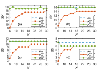
Figure 2: The distribution of estimated $\mathrm{SN}$ lower bound $\mu_{\mathrm{est}}$ of the state $\varrho_{\mathrm{iso}}^{v}$ with dimension $d=20$ as a function of the number of $N$, where (a) $v=0.95$, (b) $v=0.77$, (c) $v=0.52$, and (d) $v=0.3$. For each $N$, the expectation values of local observables are exactly calculated and the CL is $99.9\%$. After performing the $\mathrm{SN}$ estimation algorithm $N_{\mathrm{iter}}$ times, we collect $N_{\mathrm{iter}}$ estimators, $\{\mu_{\mathrm{est}}^{(i)}\}_{i=1}^{N_{\mathrm{iter}}}$, in which the minimal and maximal values are denoted as $\mu_{\mathrm{est}}^{\min}$ and $\mu_{\mathrm{est}}^{\max}$. $\mu_{\mathrm{fid}}$ denotes the $\mathrm{SN}$ estimated by the fidelity-based witness [50, 48, 49, 51].

Next, we evaluate the performance of the $\mathrm{SN}$ estimation algorithm with $N=12$ random operations. Fig. 3 displays the numerical results of the state $\varrho_{\mathrm{iso}}^{v}$ with dimension $d=20,30$ by fixing the CL $99.9\%$. In contrast, we compare our results with the $3$-MUBs criterion [34]. See the detailed construction of $3$-MUBs in Appendix B or Ref. [68]. As shown in Fig. 3(a), our approach provides a more accurate estimation of the $\mathrm{SNs}$ than the $3$-MUBs criterion for $v\leq 0.65$. For strong entanglement such as $v>0.65$, the $3$-MUBs criterion is more powerful. Similar results are obtained for $d=30$ from Fig. 3(b).

Note that the $3$-MUBs criterion for states $\varrho_{\mathrm{iso}}^{v}$ with $d=20,30$ required $60$ or $90$ projections, respectively. However, our approach uses only $5\times 12=60$ projections for $d=20,30$. Thus, our method employs fewer operations but obtains more accurate estimations for high-dimensional states with lower purity. Moreover, we compare our results with the existing optimal criterion based on the second moments [35]. For $d=20$, the optimal second moments criterion detects the state $\varrho_{\mathrm{iso}}^{v}$ as entangled for $v\geq 1/\sqrt{21}=0.2182$ [35] while our approach detect the state $\varrho_{\mathrm{iso}}^{v}$ for $v\geq 0.1$ as shown in Figs. 3(a).

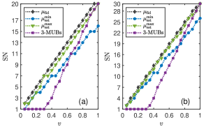
Figure 3: Numerical results for the states $\varrho_{\mathrm{iso}}^{v}$ with dimension (a) $d=20$ and (b) $d=30$ by fixing $N=12$ and the CL $99.9\%$. After performing the $\mathrm{SN}$ estimation algorithm $N_{\mathrm{iter}}$ times, we collect $N_{\mathrm{iter}}$ estimators, $\{\mu_{\mathrm{est}}^{(i)}\}_{i=1}^{N_{\mathrm{iter}}}$, in which the minimal and maximal values are denoted as $\mu_{\mathrm{est}}^{\min}$ and $\mu_{\mathrm{est}}^{\max}$. $\mu_{\mathrm{fid}}$ denotes the $\mathrm{SN}$ estimated by the fidelity-based witness. $3$-MUBs denote the results of the criterion based on the $3$ MUBs [34]. $\mu_{\mathrm{fid}}$ is the $\mathrm{SN}$ estimated by the fidelity-based witness [50, 48, 49, 51].

Remark that the above results are based on the $t$ distribution with a small sample size, $N=12$. Appendix B shows an enhanced algorithm based on the Bootstrap resample technique [63, 64, 65] to construct a confidence interval of $N=12$ and then estimate the lower bound of $\mathrm{SN}$ similar with the above algorithm. Numerical results indicate the enhanced algorithm obtains a tighter lower bound of $\mathrm{SN}$ than the original algorithm.

In Appendix C, we simulate the $\mathrm{SN}$ estimation algorithm for the state $\varrho_{\mathrm{iso}}$ with dimensions $d=40,50,60$, the noisy two-qudit purified thermal states [68], and the state $\varrho_{\mathrm{iso}}$ under random noise channel. The results indicate that $N=12$ is still sufficient to estimate the $\mathrm{SN}$ tighter than $3$-MUBs criterion, even considering the practical measurement noise of estimating the expectation values of observables.

Conclusion and outlooks.—In summary, we have introduced a criterion and a classical post-processing algorithm to estimate the Schmidt number of bipartite high-dimensional states. The proposed method offers several significant advantages. First, various experimental platforms can randomly select the measurement basis that aligns with their specific device, as long as the random operations satisfy the properties of unitary or orthogonal $2$-design. In contrast, the methods based on MUBs require that all platforms measure the state on a fixed measurement basis. It is challenging to implement MUBs for general physical platforms [69]. Second, our results rely on the first-order measurement information of observables and only require a $2$-design of unitary and orthogonal transformations. Existing high-order randomized measurements [41, 40] involve unitary $4$-design and require many random operation samples to achieve comparable precision. Finally, the proposed $\mathrm{SN}$ estimator algorithm allows for extracting more information from limited experimental data. It ensures fewer projections are sufficient to obtain a $\mathrm{SN}$ estimator of a high-dimensional entangled state. As a result, our approach saves the experimental cost, especially for high dimensional systems.

Notice that our approaches rely on the connection between the maximally entangled state and the $\mathrm{SWAP}$ operator. Therefore, it would be an interesting problem if our randomized approaches could be generalized to other entanglement witnesses for different entangled states. It would be also of significance to apply the proposed algorithm to estimate other quantities such as high-order moments in randomized measurements [35, 41, 40], Rényi entanglement entropy [70], and PT-moments [71, 72]. Moreover, one may investigate the potential of our approach to multipartite case [15]. Our results would also make it possible to experimentally characterize the entanglement of high-dimensional quantum channels [73].

Acknowledgment.—We thank Armin Tavakoli and Simon Morelli for their insightful discussions and suggestions. This work is supported by the National Natural Science Foundation of China (Grant Nos. 12125402, 12347152, 12405005, 12405006, 12075159, and 12171044), Beijing Natural Science Foundation (Grant No. Z240007), and the Innovation Program for Quantum Science and Technology (No. 2021ZD0301500), the Postdoctoral Fellowship Program of CPSF (No. GZC20230103), the China Postdoctoral Science Foundation (No. 2023M740118 and 2023M740119), the specific research fund of the Innovation Platform for Academicians of Hainan Province.

Supplemental material

In this Supplemental Material, we give more details on the theoretical results of the paper. In Appendix A, we show the proof of observation 1 in the main text. In Appendix B, we present information about the confidence interval estimation of the fidelity and the $t$-distribution. Moreover, we present an enhanced Schmidt number algorithm based on the Bootstrap resample technique [63, 64, 65]. This algorithm is suitable for small samples and does not depend on the population distribution assumption. Appendix C exhibits additional numerical results for different high-dimensional entangled states. At last, we show in Appendix D how one could estimate a lower bound of the well-known entanglement measure from the first-order moments discussed in the main text.

Appendix A Proof of the observation

Before proving the observation in the main text, we present a useful corollary showing how to calculate Haar integrals over the unitary and orthogonal groups. The proof of corollary 1 can be found in Refs. [53, 54, 55, 56].

Corollary 1.

Given $\mathcal{A}\in\mathcal{L}(\mathds{C}^{d}\otimes\mathds{C}^{d})$, we have

$$\int dU\,U^{\otimes 2}\mathcal{A}U^{{\dagger}\otimes 2} =a_{1}\mathbbm{1}_{d}\otimes\mathbbm{1}_{d}+a_{2}\mathbb{S},$$ (13)

$$\int dO\,O^{\otimes 2}\mathcal{A}O^{\top\otimes 2} =c_{1}\mathbbm{1}_{d}\otimes\mathbbm{1}_{d}+c_{2}\mathbb{S}+c_{3}\mathbb{S}^{\top_{B}},$$ (14)

where coefficients are

$$a_{1} =\frac{{\mathrm{tr}}(\mathcal{A})-d^{-1}{\mathrm{tr}}(\mathbb{S}\mathcal{A})}{d^{2}-1},$$ (15)

$$a_{2} =\frac{{\mathrm{tr}}(\mathbb{S}\mathcal{A})-d^{-1}{\mathrm{tr}}(\mathcal{A})}{d^{2}-1},$$ (16)

$$c_{1} =\frac{(d+1){\mathrm{tr}}(\mathcal{A})-{\mathrm{tr}}(\mathbb{S}\mathcal{A})-{\mathrm{tr}}(\mathbb{S}^{\top_{B}}\mathcal{A})}{d(d-1)(d+2)},$$ (17)

$$c_{2} =\frac{-{\mathrm{tr}}(\mathcal{A})+(d+1){\mathrm{tr}}(\mathbb{S}\mathcal{A})-{\mathrm{tr}}(\mathbb{S}^{\top_{B}}\mathcal{A})}{d(d-1)(d+2)},$$ (18)

$$c_{3} =\frac{-{\mathrm{tr}}(\mathcal{A})-{\mathrm{tr}}(\mathbb{S}\mathcal{A})+(d+1){\mathrm{tr}}(\mathbb{S}^{\top_{B}}\mathcal{A})}{d(d-1)(d+2)}.$$ (19)

Next, we discuss the properties of the involved four observables. Based on the main text, observables $\mathcal{M}$ and $\hat{\mathcal{M}}$ satisfy $\mathcal{M}=\mathcal{M}^{{\dagger}}$, $\hat{\mathcal{M}}=\hat{\mathcal{M}}^{{\dagger}}$, and $\hat{\mathcal{M}}=-\hat{\mathcal{M}}^{\top}$.

A.1 For rank-optimal observations

Note that observables $\mathcal{M}$ can be any observables. For simplicity, we choose $\mathcal{M}$ as a rank-$1$ projection operator, $\mathcal{M}=|j\rangle\langle j|$, where $\{|j\rangle\}$ denotes the computational bases in a $d$-dimension Hilbert space. Any antisymmetric observable $\hat{\mathcal{M}}$ satisfies the following conditions for all basis $\{|j\rangle\}_{j=1}^{d}$:

1. $\langle j|\hat{\mathcal{M}}|j\rangle=0$.

2. $\langle j|\hat{\mathcal{M}}|k\rangle=-\langle k|\hat{\mathcal{M}}|j\rangle$.

3. $\langle j|\hat{\mathcal{M}}|k\rangle=ib_{jk}$, where $i$ denotes the imaginary unit and $b_{jk}$ is a real number.

Thus, the simplest choice is that $\hat{\mathcal{M}}$ only has two nonzero elements. For example, $\hat{\mathcal{M}}=-i|j\rangle\langle k|+i|k\rangle\langle j|$ which is a rank-$2$ observable since its nonzero eigenvalues are $\pm 1$.

Now, we prove the observation 1 in the main text.

Observation 1.

For any bipartite state $\varrho$ of equal dimension $d$, the fidelity $F(\varrho)$ is given by

$$F(\varrho)=(d+1)\mathcal{R}(\varrho)-\frac{d-1}{2}\mathcal{Q}(\varrho)-\frac{1}{d}.$$ (20)

The Schmidt number of $\varrho$ is

$$\mu=\begin{cases}1,&F(\varrho)=0,\\ \lceil dF(\varrho)\rceil,&F(\varrho)\in(0,1],\\ \end{cases}$$ (21)

where the $\lceil\cdot\rceil$ is ceil function.

Proof.

Given rank-1 observables $\mathcal{M}=|j\rangle\langle j|$, we have

$${\mathrm{tr}}(\mathcal{M})=1,{\mathrm{tr}}(\mathbb{S}\mathcal{M}\otimes\mathcal{M})={\mathrm{tr}}(\mathcal{M}^{2})=1.$$ (22)

where $|j\rangle$ are computational basis of a $d$ dimension system. The moment $\mathcal{R}(\varrho)$ with observable $\mathcal{M}$ is given by

$$\mathcal{R}(\varrho) =\int dU{\mathrm{tr}}[\varrho(U\otimes U)(\mathcal{M}\otimes\mathcal{M})(U^{{\dagger}}\otimes U^{{\dagger}})]$$

$$={\mathrm{tr}}\left[\varrho\int dU(U\otimes U)(\mathcal{M}\otimes\mathcal{M})(U^{{\dagger}}\otimes U^{{\dagger}})\right]$$

$$=\frac{1}{d(d+1)}{\mathrm{tr}}\left[\varrho(\mathbbm{1}_{d}\otimes\mathbbm{1}_{d}+\mathbb{S})\right]$$ (23)

$$=\frac{1+{\mathrm{tr}}(\varrho\mathbb{S})}{d(d+1)},$$ (24)

where Eq. (23) uses Eq. (13) of corollary 1.

Constructing rank-$2$ observables $\hat{\mathcal{M}}=-i|1\rangle\langle d|+i|d\rangle\langle 1|$, we have

$${\mathrm{tr}}(\hat{\mathcal{M}}) =0,$$ (25)

$${\mathrm{tr}}(\mathbb{S}\hat{\mathcal{M}}\otimes\hat{\mathcal{M}}) ={\mathrm{tr}}(\hat{\mathcal{M}}^{2})=2,$$ (26)

$${\mathrm{tr}}(\mathbb{S}^{\top_{B}}\hat{\mathcal{M}}\otimes\hat{\mathcal{M}}) =-{\mathrm{tr}}(\hat{\mathcal{M}}^{2})=-2.$$ (27)

The moment $\mathcal{Q}(\varrho)$ with observable $\hat{\mathcal{M}}$ is given by

$$\mathcal{Q} =\int dO{\mathrm{tr}}[\varrho(O\otimes O)(\hat{\mathcal{M}}\otimes\hat{\mathcal{M}})(O^{\top}\otimes O^{\top})]$$

$$={\mathrm{tr}}\left[\varrho\int dU(O\otimes O)(\hat{\mathcal{M}}\otimes\hat{\mathcal{M}})(O^{\top}\otimes O^{\top})\right]$$

$$=\frac{2}{d(d-1)}{\mathrm{tr}}\left[\varrho(\mathbb{S}-\mathbb{S}^{\top_{B}})\right]$$ (28)

$$=\frac{2}{d(d-1)}[{\mathrm{tr}}(\varrho\mathbb{S})-{\mathrm{tr}}(\varrho\mathbb{S}^{\top_{B}})],$$ (29)

where Eq. (28) uses Eq. (14) of corollary 1 and $i=\sqrt{-1}$.

Based on Eqs. (24,29), we obtain

$${\mathrm{tr}}(\varrho\mathbb{S}^{\top_{B}}) =d(d+1)\mathcal{R}(\varrho)-\frac{d(d-1)}{2}\mathcal{Q}(\varrho)-1.$$ (30)

Notice that the fidelity-based witness is $\mathcal{W}_{\mu}=\mu\mathbbm{1}_{d}^{\otimes 2}/d-|\phi_{d}^{+}\rangle\langle\phi_{d}^{+}|$, where $|\phi_{d}^{+}\rangle=\sum_{j=1}^{d}|jj\rangle/\sqrt{d}$. For any state $\varrho$ with Schmidt number $\leq\mu$, we have ${\mathrm{tr}}(\mathcal{W}_{\mu}\varrho)\geq 0$. Recall that $|\phi_{d}^{+}\rangle$ can be expressed as

$$|\phi_{d}^{+}\rangle\langle\phi_{d}^{+}| =\frac{1}{d}\sum_{j,k=1}^{d}|j\rangle\langle k|\otimes|j\rangle\langle k|$$

$$=\frac{1}{d}\sum_{j,k=1}^{d}|j\rangle\langle k|\otimes(|k\rangle\langle j|)^{\top}=\frac{1}{d}\mathbb{S}^{\top_{B}}.$$ (31)

As a result, the fidelity for any state $\varrho$ is

$$F(\varrho) ={\mathrm{tr}}(\varrho|\phi_{d}^{+}\rangle\langle\phi_{d}^{+}|)=\frac{1}{d}{\mathrm{tr}}(\varrho\mathbb{S}^{\top_{B}})$$

$$=(d+1)\mathcal{R}(\varrho)-\frac{d-1}{2}\mathcal{Q}(\varrho)-\frac{1}{d},$$ (32)

which is the first result of observation 1.

For any state $\varrho$ with Schmidt number $\mu$,

$${\mathrm{tr}}(\mathcal{W}_{\mu}\varrho) =\frac{\mu-{\mathrm{tr}}(\varrho\mathbb{S}^{\top_{B}})}{d}=\frac{\mu}{d}-F(\varrho)\geq 0.$$ (33)

The above inequality also implies that for any state $\varrho$ with Schmidt number $\mu$ we have

$$dF(\varrho)\leq\mu.$$ (34)

Thus, we prove that the Schmidt number of $\varrho$ is

$$\mu=\begin{cases}1,&F(\varrho)=0,\\ \lceil dF(\varrho)\rceil,&F(\varrho)\in(0,1],\\ \end{cases}$$ (35)

where the $\lceil\cdot\rceil$ is ceil function. ∎

A.2 For general observables

Note that in the above analysis, we focus on well-constructed observables with rank-optimal. However, our approach is also suitable for more general observables. Suppose we construct two arbitrary observable $\mathcal{M}$, $\hat{\mathcal{M}}$ satisfying

$$\mathcal{M}=\mathcal{M}^{{\dagger}},\hat{\mathcal{M}}=-\hat{\mathcal{M}}^{\top}.$$ (36)

We perform eigenvalue decomposition for two observables

$$\mathcal{M}=VDV^{{\dagger}},\hat{\mathcal{M}}=\hat{V}\hat{D}\hat{V}^{{\dagger}},$$ (37)

where two diagonal operators,

$$D =\mathrm{diag}\left(\alpha_{1},\alpha_{2},\cdots,\alpha_{d}\right),$$ (38)

$$\hat{D} =\mathrm{diag}\left(\hat{\alpha}_{1},\hat{\alpha}_{2},\cdots,\hat{\alpha}_{d}\right),$$ (39)

and $\alpha_{i},\hat{\alpha}_{i}$ are eigenvalues. Thus, we have

$${\mathrm{tr}}(\mathcal{M}) =\sum_{i=1}^{d}\alpha_{i},$$ (40)

$${\mathrm{tr}}(\mathbb{S}\mathcal{M}\otimes\mathcal{M}) ={\mathrm{tr}}(\mathcal{M}^{2})=\sum_{i=1}^{d}\alpha_{i}^{2}.$$ (41)

The moment $\mathcal{R}(\varrho)$ with observable $\mathcal{M}$ is given by

$$\mathcal{R}(\varrho) =\int dU{\mathrm{tr}}[\varrho(U\otimes U)(\mathcal{M}\otimes\mathcal{M})(U^{{\dagger}}\otimes U^{{\dagger}})]$$

$$={\mathrm{tr}}\left[\varrho(a_{1}\mathbbm{1}_{d}\otimes\mathbbm{1}_{d}+a_{2}\mathbb{S})\right]$$

$$=a_{1}+a_{2}{\mathrm{tr}}\left[\mathbb{S}\varrho\right],$$ (42)

where coefficients are

$$a_{1} =\frac{\left(\sum_{i=1}^{d}\alpha_{i}\right)^{2}-d^{-1}\sum_{i=1}^{d}\alpha_{i}^{2}}{d^{2}-1},$$ (43)

$$a_{2} =\frac{\sum_{i=1}^{d}\alpha_{i}^{2}-d^{-1}\left(\sum_{i=1}^{d}\alpha_{i}\right)^{2}}{d^{2}-1}.$$ (44)

For observables $\hat{\mathcal{M}}$, we have

$${\mathrm{tr}}(\hat{\mathcal{M}}) =\sum_{i=1}^{d}\hat{\alpha}_{i},$$ (45)

$${\mathrm{tr}}(\mathbb{S}\hat{\mathcal{M}}\otimes\hat{\mathcal{M}}) =\sum_{i=1}^{d}\hat{\alpha}_{i}^{2},$$ (46)

$${\mathrm{tr}}(\mathbb{S}^{\top_{B}}\hat{\mathcal{M}}\otimes\hat{\mathcal{M}}) =-\sum_{i=1}^{d}\hat{\alpha}_{i}^{2}.$$ (47)

The moment $\mathcal{Q}(\varrho)$ with observable $\hat{\mathcal{M}}$ is given by

$$\mathcal{Q} =\int dO{\mathrm{tr}}[\varrho(O\otimes O)(\hat{\mathcal{M}}\otimes\hat{\mathcal{M}})(O^{\top}\otimes O^{\top})]$$

$$={\mathrm{tr}}\left[\varrho(c_{1}\mathbbm{1}_{d}\otimes\mathbbm{1}_{d}+c_{2}\mathbb{S}+c_{3}\mathbb{S}^{\top_{B}})\right]$$

$$=c_{1}+c_{2}{\mathrm{tr}}(\varrho\mathbb{S})+c_{3}{\mathrm{tr}}(\varrho\mathbb{S}^{\top_{B}}),$$ (48)

where coefficients are

$$c_{1} =\frac{(d+1)\left(\sum_{i=1}^{d}\hat{\alpha}_{i}\right)^{2}}{d(d-1)(d+2)},$$ (49)

$$c_{2} =\frac{-\left(\sum_{i=1}^{d}\hat{\alpha}_{i}\right)^{2}+(d+2)\sum_{i=1}^{d}\hat{\alpha}_{i}^{2}}{d(d-1)(d+2)},$$ (50)

$$c_{3} =\frac{-\left(\sum_{i=1}^{d}\hat{\alpha}_{i}\right)^{2}-(d+2)\sum_{i=1}^{d}\hat{\alpha}_{i}^{2}}{d(d-1)(d+2)}.$$ (51)

Based on Eqs. (42,48), we obtain

$${\mathrm{tr}}(\varrho\mathbb{S}^{\top_{B}}) =\frac{\mathcal{Q}(\varrho)}{c_{3}}-\frac{c_{1}}{c_{3}}-\frac{c_{2}\left[\mathcal{R}(\varrho)-a_{1}\right]}{c_{3}}.$$ (52)

Finally, the fidelity is

$$F(\varrho) =\frac{{\mathrm{tr}}(\varrho\mathbb{S}^{\top_{B}})}{d}$$

$$=\frac{\mathcal{Q}(\varrho)}{dc_{3}}-\frac{c_{1}}{dc_{3}}-\frac{c_{2}\left[\mathcal{R}(\varrho)-a_{1}\right]}{dc_{3}}.$$ (53)

With the above equation, we estimate the $\mathrm{SN}$ by the fidelity-based witness.

In particular, for the rank-optimal observables constructed before, $\alpha_{1}=1,\alpha_{i}=0$ for $i=2,\cdots,d$ and $\hat{\alpha}_{1}=1,\hat{\alpha}_{2}=-1,\hat{\alpha}_{i}=0$ for $i=3,\cdots,d$. Thus, the parameters are

$$a_{1} =a_{2}=\frac{1}{d(d+1)},$$

$$c_{1} =0,c_{2}=\frac{2}{d(d-1)}=-c_{3}.$$ (54)

Putting the above parameters into Eq. (53), the corresponding fidelity is in agreement with the result in the main text.

Appendix B Confidence interval for the mean and the bootstrapping resample technique

Suppose we are interested in a population and want to figure out the population parameter such as the mean of the population. But we have no prior on the distribution of the population. Generally, we assume the distribution of the population is a normal distribution with unknown mean $g$ and the unknown deviation $\sigma$. But, you can obtain a data set $X=\{X_{j}\}_{j=1}^{N}$ with $N$ samples randomly generated from the population. The goal is to estimate a range of the unknown mean $g$ from the sample $X=\{X_{j}\}_{j=1}^{N}$.

First, we can calculate the sample mean $\bar{X}=\mathbb{E}[x]=\frac{1}{N}\sum_{j=1}^{N}X_{j}$, which is a point estimation of the mean $g$. Then the confidence interval is constructed by

$$\bar{X}\pm t_{\alpha,N-1}\frac{s}{\sqrt{N}}.$$ (55)

Here, $s=\sqrt{\frac{\sum_{j=1}^{N}\left(X_{j}-\bar{X}\right)^{2}}{N-1}}$ is the sample standard deviation, and the critical factor $t_{\alpha,N-1}$ comes from the $t$-distribution. Note that $t_{\alpha,N-1}$ depends on the confidence level $\alpha$ and sample size $N$. For example, $t_{95\%,11}\neq t_{95\%,20}$.

The central limit Theorem [60, 61] states that for sample size $N\geq 30$, the sample mean $\mathbb{E}[x]$ is approximately normally distributed, with mean $g$ and standard deviation $\sigma(\bar{X})=\frac{\sigma}{\sqrt{N}}$. Regardless of the distribution of the population, as the sample size is increased the sampling distribution of the sample mean becomes a normal distribution. That is we can always obtain a confidence interval with sample size $N\geq 30$ and the population distribution is not important.

However, for a small sample size $N<30$, the confidence interval is only efficient when the population distribution is normal. If the assumption is violated, the constructed confidence interval may be inaccurate.

Two of the traditional methods for obtaining a confidence interval for the mean of a non-normal distribution are the central limit theorem [60, 61], reported above, and the bootstrap resampling technique [63, 64, 65]. The bootstrap resampling technique is a popular non-parametric method and is useful for small sample sizes. The detailed process is the following [63, 64, 65, 62, 74].

Input: Given a data set $X=\{X_{j}\}_{j=1}^{N}$ with $N$ samples randomly generated from the population. Generally, $N<30$.

Step 1. Resample the observed sample with replacement and calculate the sample mean for this bootstrap sample.

Step 2. Repeat Step 1. $B$ times.

Output: Construct the confidence interval for the data set with size $B$ by using the Eq. (55).

In the main text, we would like to calculate the fidelity

$$F(\varrho) =(d+1)\mathcal{R}(\varrho)-\frac{d-1}{2}\mathcal{Q}(\varrho)-\frac{1}{d}$$

$$=(d+1)\int dUE_{U}(\varrho)-\frac{d-1}{2}\int dOE_{O}(\varrho)-\frac{1}{d}$$

$$=\int dWF_{W}(\varrho),$$ (56)

where the quantity

$$F_{W}(\varrho)=(d+1)E_{U}(\varrho)-\frac{d-1}{2}E_{O}(\varrho)-\frac{1}{d}.$$ (57)

We can treat the fidelity $F(\varrho)$ as a mean of an unknown population. Thus, we can estimate the fidelity $F(\varrho)$ from a statistical view. After sampling $N$ random unitaries and random orthogonal transformations, we obtain $n$ fidelities estimated by one unitary and one orthogonal transformation. Except for obtaining a point estimation from finite samples, we also try to construct a confidence interval of the unknown mean, $F(\varrho)$. The construction approach follows the Eq. (55).

Note that the population distribution with mean $F(\varrho)$ is unknown and thus we are not sure whether it is normal or not. Hence, direct construction from Eq. (55) requires the number of sample $\geq 30$. However, in our case, measuring the expectation values for large $N$ is challenging. Thus, it is preferred to estimate a few random operations, such as $N<30$. Due to the population distribution being unknown, the constructed confidence interval for $N<30$ may be inaccurate. Fortunately, numerical results indicate that this direct construction works well. The estimated $\mathrm{SNs}$ is a true lower bound of the exact $\mathrm{SNs}$.

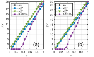
Figure C6: Test for algorithm based on Bootstrapping resampling technique. Numerical results for the states $\varrho_{\mathrm{iso}}^{v}$ with dimension (a) $d=20$ and (b) $d=30$ by fixing $N=12$ and the CL $99.9\%$. We set the number of resampling $B=5000$. After performing the $\mathrm{SN}$ estimation algorithm $N_{\mathrm{iter}}=2000$ times, we collect $N_{\mathrm{iter}}$ estimators, $\{\mu_{\mathrm{est}}^{(i)}\}_{i=1}^{N_{\mathrm{iter}}}$, in which the minimal and maximal values are denoted as $\mu_{\mathrm{est}}^{\min}$ and $\mu_{\mathrm{est}}^{\max}$. $\mu_{\mathrm{fid}}$ denotes the $\mathrm{SN}$ estimated by the fidelity-based witness. $3$-MUBs denote the results of the criterion based on the $3$ MUBs [34].

Here, we employ the Bootstrap resample technique [63, 64, 65] to construct a confidence interval of $N=12$ and then estimate the lower bound of $\mathrm{SN}$. As shown in Fig. C6, the enhanced algorithm obtains a tighter lower bound of the $\mathrm{SN}$. It is better than the original algorithm in the main text.

Appendix C Analysis of numerical results

In this section, we review the $3$-MUBs criterion [34] and the randomized measurements [40, 41] for detecting the Schmidt number.

The $3$-MUBs criterion [34] employes $3$-MUBs to estimate the $\mathrm{SNs}$. For any dimensions, reference [68] constructs the following $3$ MUBs, $\{|e_{a}^{1}\rangle=|a\rangle\}_{a=0}^{d-1}$, $\{|e_{a}^{2}\rangle\}_{a=0}^{d-1}$, and $\{|e_{a}^{3}\rangle\}_{a=0}^{d-1}$ with

$$|e_{a}^{2}\rangle =\frac{1}{\sqrt{d}}\sum_{j=1}^{d}e^{2\pi i\left(\frac{\alpha j^{2}}{2d}+\frac{aj}{2d}\right)}|j\rangle,$$ (58)

$$|e_{a}^{3}\rangle =\frac{1}{\sqrt{d}}\sum_{j=1}^{d}e^{2\pi i\left(\frac{(\alpha+d-1)j^{2}}{2d}+\frac{aj}{2d}\right)}|j\rangle.$$ (59)

Based on the criterion in [34], for any bipartite state $\varrho$ with dimension $d$ and $\mathrm{SN}$ at most $\mu$ it hold that

$$\mathcal{S}_{3,d}(\varrho)\leq 1+\frac{2\mu}{d},$$ (60)

where the quantity

$$\mathcal{S}_{3,d}(\varrho)=\sum_{z=1}^{3}\sum_{a=1}^{d}{\mathrm{tr}}\left[\varrho|e_{a}^{z}\rangle\langle e_{a}^{z}|\otimes|e_{a}^{z*}\rangle\langle e_{a}^{z*}|\right].$$ (61)

It is clear from Eq. (61) that the total number of projections required to perform $3$ MUBs is $3d$ which scales linearly with dimension $d$. In contrast, our approach requires $5N$ projections independent of dimension $d$, where $N$ represents the number of random unitary or orthogonal transformations.

The randomized measurements obtain the quantity

$$R^{(t)}=\int dU_{A}\int dU_{B}E_{AB}^{t},$$ (62)

where $t$ is an integer and the expectation value is defined as

$$E_{AB}={\mathrm{tr}}\left[(U_{A}\otimes U_{B})\varrho(U_{A}^{{\dagger}}\otimes U_{B}^{{\dagger}})(G_{A}\otimes G_{B})\right],$$ (63)

for some well-defined observables $G_{A}$ and $G_{B}$. The random unitary $U_{A}$ and $U_{B}$ are sampled via the Haar measure on the unitary group [44, 45, 46, 47].

Second, we consider the decomposition of $\varrho$ in terms of the Gell-Mann matrices

$$\varrho=\frac{1}{d^{2}} \left[\mathbbm{1}_{d}\otimes\mathbbm{1}_{d}+\sum_{j=1}^{d^{2}-1}\alpha_{j}\lambda_{j}\otimes\mathbbm{1}_{d}+\sum_{k=1}^{d^{2}-1}\mathbbm{1}_{d}\otimes\beta_{k}\lambda_{k}\right.$$

$$\left.+\sum_{j,k=1}^{d^{2}-1}T_{jk}\lambda_{j}\otimes\lambda_{k}\right].$$ (64)

In this way, the reduced states are

$$\varrho_{A} ={\mathrm{tr}}_{B}(\varrho)=\frac{1}{d}\left(\mathbbm{1}_{d}+\sum_{j=1}^{d^{2}-1}\alpha_{j}\lambda_{j}\right),$$ (65)

$$\varrho_{B} ={\mathrm{tr}}_{B}(\varrho)=\frac{1}{d}\left(\mathbbm{1}_{d}+\sum_{k=1}^{d^{2}-1}\beta_{k}\lambda_{k}\right).$$ (66)

We define the correlation matrix $T=(T_{jk})$ for $j,k=1,\cdots,d^{2}-1$. In particular, we have

$${\mathrm{tr}}(\varrho^{2}) =\frac{1}{d^{2}}\Big{(}1+\sum_{j=1}^{d^{2}-1}\alpha_{j}^{2}+\sum_{k=1}^{d^{2}-1}\beta_{k}^{2}+\sum_{j,k=1}^{d^{2}-1}T_{jk}^{2}\Big{)},$$ (67)

$${\mathrm{tr}}(\varrho_{A}^{2}) =\frac{1}{d}\Big{(}1+\sum_{j=1}^{d^{2}-1}\alpha_{j}^{2}\Big{)},{\mathrm{tr}}(\varrho_{B}^{2})=\frac{1}{d}\Big{(}1+\sum_{k=1}^{d^{2}-1}\beta_{k}^{2}\Big{)},$$ (68)

and then

$${\mathrm{tr}}(\varrho^{2})=\frac{1}{d^{2}}\Big{[}d{\mathrm{tr}}(\varrho_{A}^{2})+d{\mathrm{tr}}(\varrho_{B}^{2})-1+\sum_{j,k=1}^{d^{2}-1}T_{jk}^{2}\Big{]}.$$ (69)

It is clear to see that

$$\|T\|_{{\mathrm{tr}}}^{2} =\sum_{j,k=1}^{d^{2}-1}T_{jk}^{2}$$ (70)

$$=d^{2}{\mathrm{tr}}(\varrho^{2})-d{\mathrm{tr}}(\varrho_{A}^{2})-d{\mathrm{tr}}(\varrho_{B}^{2})+1.$$ (71)

Note that each purities ${\mathrm{tr}}(\varrho^{2})$, ${\mathrm{tr}}(\varrho_{A}^{2})$, and ${\mathrm{tr}}(\varrho_{B}^{2})$ can be accessed by the second moments $R^{(2)}$.

The criterion based on the second moments is constructed by calculating the second moments of the $d\otimes d$ state $|\phi_{+}^{\mu}\rangle=\frac{1}{\sqrt{\mu}}\sum_{j=0}^{\mu-1}|jj\rangle$. For $\mu=1,2,\cdots,d$, we obtain a data set

$$\left[R^{(2)}(|\phi_{+}^{1}\rangle\langle\phi_{+}^{1}|),\cdots,R^{(2)}(|\phi_{+}^{d}\rangle\langle\phi_{+}^{d}|)\right].$$ (72)

Then given a state $\varrho$ if $R^{(2)}(\varrho)\leq R^{(2)}(|\phi_{+}^{\mu}\rangle\langle\phi_{+}^{\mu}|)$ for $\mu\in[1,d-1]$ then $\varrho$ has a Schmidt number $\mu$. If $R^{(2)}(\varrho)>R^{(2)}(|\phi_{+}^{d-1}\rangle\langle\phi_{+}^{d-1}|)$, then $\varrho$ has a Schmidt number $d$. See details in Refs. [35, 40, 41]. We call this criterion $2$-RMs as shown in Fig. C4(a).

The purified thermal states mixed with white noise is

$$\varrho_{\mathrm{thermal}}(v,\beta)=v|\psi(\beta)\rangle\langle\psi(\beta)|+\frac{v}{d^{2}}\mathbbm{1}_{d^{2}},$$ (73)

where $v\in[0,1]$ and the pure state

$$|\psi(\beta)\rangle=\frac{1}{\sqrt{\sum_{j=1}^{d}e^{-\beta j}}}\sum_{j=1}^{d}e^{-\beta j}|jj\rangle.$$ (74)

Furthermore, we consider the random noise state

$$\varrho_{\mathrm{rand}}^{v}(\sigma) =v|\phi_{d}^{+}\rangle\langle\phi_{d}^{+}|+(1-v)\sigma,$$ (75)

where $v\in[0,1]$ and the random states $\sigma$ is sampled according to the Hilbert-Schmidt metric [75].

Finally, we simulate the performance of the $\mathrm{SN}$ estimation algorithm in an experimental scenario. Note that in the main text, we iteratively run the $\mathrm{SN}$ estimation algorithm $N_{\mathrm{iter}}$ times for a fixed $N$. However, in an experimental scenario, we only obtain a few data by sampling $N$ random unitaries and $N$ random orthogonal transformations. This process only performs the $\mathrm{SN}$ estimation algorithm one time. In the following simulations, we set the number of measurements for local observables as $M=100d$. Fig. C4 and C5 display additional numerical results for different states. These results suggest that $N=12$ is efficient for high dimensions and exhibits significant advantages compared with the $3$-MUBs criterion and the secon-order moment from randomized measurements.

The code of generating random unitaries and orthogonal transformations can be found in the link: "http://www.qetlab.com/RandomUnitary".

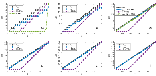
Figure C4: Numerical results for the states $\varrho_{\mathrm{iso}}^{v}$ with dimension (a) $d=10$, (b) $d=15$, (c) $d=40$, (d) $d=50$, (e) $d=60$, (f) $d=80$. For (a,b), the number of measurements for each local observable is $M=100d$. For (c-f), we directly calculate the expectation values of observables. In (a,b,d,e,f), the CL is $99\%$.

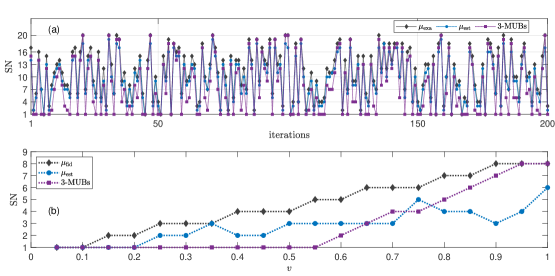
Figure C5: (a) shows the numerical results for the states $\varrho_{\mathrm{rand}}^{v}$ with dimension $d=20$. The parameter $v\in[0,1]$ and the state $\sigma$ are random for each iteration. The number of measurements for each local observable is $M=100d$ and the CL is $99\%$. (b) shows the results for the noisy two-qudit purified thermal states $\varrho_{\mathrm{thermal}}(v,\beta)$ with dimension $d=20$ and the parameter $\beta=0.5$.

Appendix D The entanglement quantification

Here, we show that the moments $\mathcal{R}(\varrho)$ and $\mathcal{Q}(\varrho)$, Eq. (2), induce lower bounds of entanglement measures in quantum information.

An important entanglement measure is based on the trace distance, $E_{T}(\varrho)=\min_{\sigma\in\mathrm{SEP}}D_{T}(\varrho,\sigma)$, given by the smallest trace distance between $\varrho$ and separable state set $\mathrm{SEP}$ [66], where the trace distance is defined as half of the trace norm, $D_{T}(\varrho,\sigma)=\frac{1}{2}\|\varrho-\sigma\|_{{\mathrm{tr}}}$, and $\|C\|_{{\mathrm{tr}}}$ denotes the trace norm of $C$, i.e., the sum of the absolute values of eigenvalues of $C$. We present our results as follows.

Observation 2.

For any bipartite state $\varrho$ of equal dimension $d$, the entanglement measure based on the trace distance $E_{T}(\varrho)$ has a lower bound,

$$E_{T}(\varrho)\geq(d+1)\mathcal{R}(\varrho)-\frac{d-1}{2}\mathcal{Q}(\varrho)-\frac{2}{d}.$$ (76)

Proof.

Let $\sigma_{\mathrm{opt}}$ be the closest separable state. We have the inequality, $E_{T}(\varrho)=\frac{1}{2}\|\varrho-\sigma_{\mathrm{opt}}\|_{1}\geq\frac{1}{2}|{\mathrm{tr}}[(\varrho-\sigma_{\mathrm{opt}})]|\geq\frac{1}{2}|{\mathrm{tr}}[(\varrho-\sigma_{\mathrm{opt}})\mathcal{W}_{1}^{{}^{\prime}}]|\geq-{\mathrm{tr}}(\varrho\mathcal{W}_{1})$, where $\mathcal{W}_{1}=\mathbbm{1}_{d}^{\otimes 2}/d-|\phi_{d}^{+}\rangle\langle\phi_{d}^{+}|$ is the fidelity-based entanglement witness [49] and $\mathcal{W}_{1}^{{}^{\prime}}=2\mathcal{W}_{1}-(\frac{2}{d}-1)\mathbbm{1}_{d}^{\otimes^{2}}$. The first inequality holds due to the absolute value inequality. The second inequality is true since the absolute values of the eigenvalues of $\mathcal{W}_{1}^{{}^{\prime}}$ are equal to one. The third inequality is based on the property of the entanglement witness $\mathcal{W}_{1}$. By expressing ${\mathrm{tr}}(\varrho\mathcal{W}_{1})$ in terms of $\mathcal{R}(\varrho)$ and $\mathcal{Q}(\varrho)$ based on observation 1, we complete the proof. ∎

Following the Refs. [76, 77], other entanglement measures such as the concurrence [78], the G-concurrence [79], the entanglement of formation [80], the geometric measure of entanglement [81], and the robustness of entanglement [82] have a connection with the entanglement witness $\mathcal{W}_{1}$. Thus, these entanglement measures can also be bounded by a function of $\mathcal{R}(\varrho)$ and $\mathcal{Q}(\varrho)$.

References

- Scarani et al. [2009] V. Scarani, H. Bechmann-Pasquinucci, N. J. Cerf, M. Dušek, N. Lütkenhaus, and M. Peev, Rev. Mod. Phys. 81, 1301 (2009).
- Xu et al. [2020] F. Xu, X. Ma, Q. Zhang, H.-K. Lo, and J.-W. Pan, Rev. Mod. Phys. 92, 025002 (2020).
- Pirandola et al. [2020] S. Pirandola, U. L. Andersen, L. Banchi, M. Berta, D. Bunandar, R. Colbeck, D. Englund, T. Gehring, C. Lupo, C. Ottaviani, et al., Adv. Opt. Photonics 12, 1012 (2020).
- Giovannetti et al. [2011] V. Giovannetti, S. Lloyd, and L. Maccone, Nat. Photonics 5, 222 (2011).
- Degen et al. [2017] C. L. Degen, F. Reinhard, and P. Cappellaro, Rev. Mod. Phys. 89, 035002 (2017).
- Tóth and Apellaniz [2014] G. Tóth and I. Apellaniz, J. Phys. A: Math. Theor. 47, 424006 (2014).
- Amico et al. [2008] L. Amico, R. Fazio, A. Osterloh, and V. Vedral, Rev. Mod. Phys. 80, 517 (2008).
- Zhao et al. [2024] Q. Zhao, Y. Zhou, and A. M. Childs, arXiv preprint arXiv:2406.02379 (2024).
- Erhard et al. [2020] M. Erhard, M. Krenn, and A. Zeilinger, Nat. Rev. Phys. 2, 365 (2020).
- Dada et al. [2011] A. C. Dada, J. Leach, G. S. Buller, M. J. Padgett, and E. Andersson, Nature Phys. 7, 677 (2011).
- Nape et al. [2021] I. Nape, V. Rodríguez-Fajardo, F. Zhu, H.-C. Huang, J. Leach, and A. Forbes, Nat. Commun. 12, 5159 (2021).
- Tabia et al. [2022] G. N. M. Tabia, V. S. R. Bavana, S.-X. Yang, and Y.-C. Liang, Phys. Rev. A 106, 012209 (2022).
- D’Alessandro et al. [2024] N. D’Alessandro, A. Tavakoli, et al., arXiv preprint arXiv:2410.02554 (2024).
- Tavakoli and Morelli [2024] A. Tavakoli and S. Morelli, Phys. Rev. A 110, 062417 (2024).
- Cobucci and Tavakoli [2024] G. Cobucci and A. Tavakoli, Sci. Adv. 10, eadq4467 (2024).
- Liu et al. [2024] S. Liu, Q. He, M. Huber, and G. Vitagliano, arXiv preprint arXiv:2405.03261 (2024).
- Yan et al. [2013] B. Yan, S. A. Moses, B. Gadway, J. P. Covey, K. R. Hazzard, A. M. Rey, D. S. Jin, and J. Ye, Nature 501, 521 (2013).
- Parigi et al. [2015] V. Parigi, V. D’Ambrosio, C. Arnold, L. Marrucci, F. Sciarrino, and J. Laurat, Nat. Commun. 6, 7706 (2015).
- Senko et al. [2015] C. Senko, P. Richerme, J. Smith, A. Lee, I. Cohen, A. Retzker, and C. Monroe, Phys. Rev. X 5, 021026 (2015).
- Mair et al. [2001] A. Mair, A. Vaziri, G. Weihs, and A. Zeilinger, Nature 412, 313 (2001).
- Wang et al. [2012] J. Wang, J.-Y. Yang, I. M. Fazal, N. Ahmed, Y. Yan, H. Huang, Y. Ren, Y. Yue, S. Dolinar, M. Tur, et al., Nat. photonics 6, 488 (2012).
- Krenn et al. [2016] M. Krenn, M. Malik, R. Fickler, R. Lapkiewicz, and A. Zeilinger, Phys. Rev. Lett. 116, 090405 (2016).
- Valencia et al. [2020] N. H. Valencia, V. Srivastav, M. Pivoluska, M. Huber, N. Friis, W. McCutcheon, and M. Malik, Quantum 4, 376 (2020).
- Vértesi et al. [2010] T. Vértesi, S. Pironio, and N. Brunner, Phys. Rev. Lett. 104, 060401 (2010).
- Cerf et al. [2002] N. J. Cerf, M. Bourennane, A. Karlsson, and N. Gisin, Phys. Rev. Lett. 88, 127902 (2002).
- Zhu et al. [2021] F. Zhu, M. Tyler, N. H. Valencia, M. Malik, and J. Leach, AVS Quantum Sci. 3, 011401 (2021).
- Gühne and Tóth [2009] O. Gühne and G. Tóth, Phys. Rep. 474, 1 (2009).
- Zhang et al. [2024] C. Zhang, S. Denker, A. Asadian, and O. Gühne, Phys. Rev. Lett. 133, 040203 (2024).
- Bavaresco et al. [2018] J. Bavaresco, N. Herrera Valencia, C. Klöckl, M. Pivoluska, P. Erker, N. Friis, M. Malik, and M. Huber, Nat. Phys. 14, 1032 (2018).
- Wootters and Fields [1989] W. K. Wootters and B. D. Fields, Ann. Phys. 191, 363 (1989).
- Ivonovic [1981] I. Ivonovic, J. Phys. A: Math. Gen. 14, 3241 (1981).
- Brierley and Weigert [2010] S. Brierley and S. Weigert, in J. Phys. Conf. Ser., Vol. 254 (IOP Publishing, 2010) p. 012008.
- Durt [2005] T. Durt, J. Phys. A 38, 5267 (2005).
- Morelli et al. [2023] S. Morelli, M. Huber, and A. Tavakoli, Phys. Rev. Lett. 131, 170201 (2023).
- Imai et al. [2021] S. Imai, N. Wyderka, A. Ketterer, and O. Gühne, Phys. Rev. Lett. 126, 150501 (2021).
- Liu et al. [2022] Z. Liu, P. Zeng, Y. Zhou, and M. Gu, Phys. Rev. A 105, 022407 (2022).
- Wyderka et al. [2023a] N. Wyderka, A. Ketterer, S. Imai, J. L. Bönsel, D. E. Jones, B. T. Kirby, X.-D. Yu, and O. Gühne, Phys. Rev. Lett. 131, 090201 (2023a).
- Imai et al. [2024] S. Imai, G. Tóth, and O. Gühne, Phys. Rev. Lett. 133, 060203 (2024).
- Cieśliński et al. [2024] P. Cieśliński, S. Imai, J. Dziewior, O. Gühne, L. Knips, W. Laskowski, J. Meinecke, T. Paterek, and T. Vértesi, Phys. Rep. 1095, 1 (2024).
- Liu et al. [2023] S. Liu, Q. He, M. Huber, O. Gühne, and G. Vitagliano, PRX Quantum 4, 020324 (2023).
- Wyderka and Ketterer [2023] N. Wyderka and A. Ketterer, PRX Quantum 4, 020325 (2023).
- Adamson and Steinberg [2010] R. B. A. Adamson and A. M. Steinberg, Phys. Rev. Lett. 105, 030406 (2010).
- Lib et al. [2024] O. Lib, S. Liu, R. Shekel, Q. He, M. Huber, Y. Bromberg, and G. Vitagliano, arXiv preprint arXiv:2412.04643 (2024).
- Goodman and Wallach [2000] R. Goodman and N. R. Wallach, Representations and invariants of the classical groups (Cambridge University Press, 2000).
- Collins and Śniady [2006] B. Collins and P. Śniady, Commun. Math. Phys. 264, 773 (2006).
- Gross et al. [2007] D. Gross, K. Audenaert, and J. Eisert, J. Math. Phys. 48, 052104 (2007).
- Dankert et al. [2009] C. Dankert, R. Cleve, J. Emerson, and E. Livine, Phys. Rev. A 80, 012304 (2009).
- Sanpera et al. [2001] A. Sanpera, D. Bruß, and M. Lewenstein, Phys. Rev. A 63, 050301 (2001).
- Gühne et al. [2021] O. Gühne, Y. Mao, and X.-D. Yu, Phys. Rev. Lett. 126, 140503 (2021).
- Terhal and Horodecki [2000] B. M. Terhal and P. Horodecki, Phys. Rev. A 61, 040301 (2000).
- Wyderka et al. [2023b] N. Wyderka, G. Chesi, H. Kampermann, C. Macchiavello, and D. Bruß, Phys. Rev. A 107, 022431 (2023b).
- Van Kirk et al. [2022] K. Van Kirk, J. Cotler, H.-Y. Huang, and M. D. Lukin, arXiv preprint arXiv:2212.06084 (2022).
- Mele [2024] A. A. Mele, Quantum 8, 1340 (2024).
- Hashagen et al. [2018] A. Hashagen, S. Flammia, D. Gross, and J. Wallman, Quantum 2, 85 (2018).
- García-Martín et al. [2023] D. García-Martín, M. Larocca, and M. Cerezo, arXiv preprint arXiv:2305.09957 (2023).
- Liang et al. [2024] J.-M. Liang, S. Imai, S. Liu, S.-M. Fei, O. Gühne, and Q. He, arXiv preprint arXiv:2411.06013 (2024).
- Student [1908] Student, Biometrika , 1 (1908).
- Bonett and Seier [2003] D. G. Bonett and E. Seier, Amer. Statist. 57, 233 (2003).
- Montgomery and Runger [2010] D. C. Montgomery and G. C. Runger, Applied statistics and probability for engineers (John wiley & sons, 2010).
- Rosenblatt [1956] M. Rosenblatt, Proc. Natl. Acad. Sci 42, 43 (1956).
- Bellhouse [2001] D. R. Bellhouse, Am. Stat. 55, 352 (2001).
- Wang [2001] F.-K. Wang, Quality and Reliability Engineering International 17, 257 (2001).
- Efron [1992] B. Efron, in Breakthroughs in statistics: Methodology and distribution (Springer, 1992) pp. 569–593.
- Efron [1982] B. Efron, The jackknife, the bootstrap and other resampling plans (SIAM, 1982).
- Efron and Tibshirani [1994] B. Efron and R. J. Tibshirani, An introduction to the bootstrap (Chapman and Hall/CRC, 1994).
- Nielsen and Chuang [2010] M. A. Nielsen and I. L. Chuang, Quantum computation and quantum information (Cambridge university press, 2010).
- [67] In our numerical simulation, we always set .
- Li et al. [2024] N. K. H. Li, M. Huber, and N. Friis, arXiv preprint arXiv:2406.04395 (2024).
- Euler and Gärttner [2023] N. Euler and M. Gärttner, PRX Quantum 4, 040338 (2023).
- Brydges et al. [2019] T. Brydges, A. Elben, P. Jurcevic, B. Vermersch, C. Maier, B. P. Lanyon, P. Zoller, R. Blatt, and C. F. Roos, Science 364, 260 (2019).
- Elben et al. [2020] A. Elben, R. Kueng, H.-Y. R. Huang, R. van Bijnen, C. Kokail, M. Dalmonte, P. Calabrese, B. Kraus, J. Preskill, P. Zoller, and B. Vermersch, Phys. Rev. Lett. 125, 200501 (2020).
- Yu et al. [2021] X.-D. Yu, S. Imai, and O. Gühne, Phys. Rev. Lett. 127, 060504 (2021).
- Engineer et al. [2024] S. Engineer, S. Goel, S. Egelhaaf, W. McCutcheon, V. Srivastav, S. Leedumrongwatthanakun, S. Wollmann, B. Jones, T. Cope, N. Brunner, et al., arXiv preprint arXiv:2408.15880 (2024).
- Pek et al. [2017] J. Pek, A. C. Wong, and O. C. Wong, Open J. Stat. 7, 405 (2017).
- Życzkowski and Sommers [2005] K. Życzkowski and H.-J. Sommers, Phys. Rev. A 71, 032313 (2005).
- Zhang et al. [2016] C. Zhang, S. Yu, Q. Chen, H. Yuan, and C. H. Oh, Phys. Rev. A 94, 042325 (2016).
- Sun et al. [2024] L.-L. Sun, X. Zhou, A. Tavakoli, Z.-P. Xu, and S. Yu, Phys. Rev. Lett. 132, 110204 (2024).
- Wootters [1998] W. K. Wootters, Phys. Rev. Lett. 80, 2245 (1998).
- Gour [2005] G. Gour, Phys. Rev. A 71, 012318 (2005).
- Wootters [2001] W. K. Wootters, Quantum Inf. Comput. 1, 27 (2001).
- Wei and Goldbart [2003] T.-C. Wei and P. M. Goldbart, Phys. Rev. A 68, 042307 (2003).
- Vidal and Tarrach [1999] G. Vidal and R. Tarrach, Phys. Rev. A 59, 141 (1999).