Bridging Simplicity and Sophistication using GLinear: A Novel Architecture for Enhanced Time Series Prediction

Abstract

Time Series Forecasting (TSF) is an important application across many fields. There is a debate about whether Transformers, despite being good at understanding long sequences, struggle with preserving temporal relationships in time series data. Recent research suggests that simpler linear models might outperform or at least provide competitive performance compared to complex Transformer-based models for TSF tasks. In this paper, we propose a novel data-efficient architecture, GLinear, for multivariate TSF that exploits periodic patterns to provide better accuracy. It also provides better prediction accuracy by using a smaller amount of historical data compared to other state-of-the-art linear predictors. Four different datasets (ETTh1, Electricity, Traffic, and Weather) are used to evaluate the performance of the proposed predictor. A performance comparison with state-of-the-art linear architectures (such as NLinear, DLinear, and RLinear) and transformer-based time series predictor (Autoformer) shows that the GLinear, despite being parametrically efficient, significantly outperforms the existing architectures in most cases of multivariate TSF. We hope that the proposed GLinear opens new fronts of research and development of simpler and more sophisticated architectures for data and computationally efficient time-series analysis. The source code is publicly available on GitHub.

I Introduction

Accurate forecasting has become increasingly valuable in today’s data-driven world, where computational intelligence is key to automated decision-making [10, 18]. Time Series Forecasting (TSF) tasks have various applications that impact diverse fields such as finance, healthcare, supply chain management, and climate science [12]. The ability to predict future trends based on historical data not only enhances decision-making processes, but also drives innovation and operational efficiency.

Forecasting is typically categorized into short-term, medium-term, and long-term predictions, each serving distinct purposes and employing tailored methodologies [17]. Short-term forecasting focuses on immediate needs; medium-term forecasting assists in strategic planning, while long-term forecasting aids in vision-setting and resource allocation [13]. Historically, traditional statistical methods like exponential smoothing [13] and ARIMA [15] have dominated the forecasting arena for short-term TSF. Traditional methods capture trend and seasonality components in the data and perform well due to their simplicity and responsiveness to recent data [16, 18]. However, they struggle with medium- and long-term predictions, and this decline can be attributed to assumptions of linearity and stationarity, often leading to overfitting and limited adaptability [19, 20].

The emergence of advanced and hybrid methods that use Deep Learning (DL), have revolutionized predictive modeling by enabling the extraction of complex patterns within the data [34]. Recurrent Neural Networks (RNNs), Long Short Term Memory (LSTM), and Transformer-based architectures have shown promising results in medium- and long-term forecasting without rigid assumptions [21, 1, 22]. Despite their sophistication, recent studies indicate that linear models can capture periodic patterns and provide competitive performance in certain contexts along with computational efficiency [1, 2].

Not all time-series data are suitable for precise predictions, particularly when it comes to long-term forecasting, which becomes especially difficult in chaotic systems [2]. Long-term forecasting has been shown to be most feasible for time series data when data exhibits clear trends and periodic patterns  [2, 1]. This brings up a question: How can we effectively integrate the simplicity of linear models with sophisticated techniques for capturing complex underlying patterns to further enhance medium- and long-term TSF?

Among popular linear models, NLinear [1] often struggles with non-linear relationships in data, leading to suboptimal performance in complex forecasting scenarios. On the other hand, DLinear [1] is computationally intensive and may require large amounts of training data, which can hinder real-time application and scalability. Although RLinear [2] models are capable of capturing trends and seasonality, they often fall short in their ability to generalize across varying datasets.

Inspired from long TSF linear models (NLinear, DLinear and RLinear); we propose a novel data-efficient architecture, GLinear. GLinear is a simple model that does not have any complex components, functions, or blocks (like self-attention schemes, positional encoding blocks, etc.) like previously mentioned linear models. It has capabilities of enhanced forecasting performance while maintaining simplicity. Furthermore, GLinear focuses on data efficiency and demonstrates the potential to perform robust forecasting without relying on extensive historical datasets, which is a common limitation of other TSF models. Our contributions in this paper are outlined as follows:

• We propose a novel architecture, GLinear that can deliver highly accurate TSF by leveraging periodic patterns, making it a promising solution for diverse forecasting applications.

• We rigorously perform experiments to validate the GLinear architecture through empirical experiments comparing its performance against state-of-the-art methods.

• We explore GLinear’s applicability across diverse sectors, assessing its impact on forecasting performance with varying data input length and the prediction horizons.

The remainder of the paper is organized as follows: Section II presents related work on TSF using state-of-the-art transformer-based models and linear predictors along with their limitations. Section III presents the architecture of different linear models to provide a better understanding of the proposed method. Section IV presents the proposed GLinear model. Section V presents the detail of experimental setup including used datasets, implementation details and evaluation metrics. Different experiments and their results are presented in Section VI. Finally, Section VII concludes our research with takeaways and future directions.

II Related Work

TSF has become increasingly crucial due to its wide range of real-world applications. Consequently, diverse methodologies have been developed to improve prediction accuracy and robustness. Recent research has explored both simpler (traditional) and complex (DL-based) approaches. One prominent direction leverages the power of multi-head attention mechanisms within Transformer architectures to capture intricate temporal dependencies [23, 24, 25]. In contrast, other studies [30, 1, 2] have demonstrated the effectiveness of simpler, computationally efficient models, such as single-layer linear models, for certain forecasting tasks.

II-A State-of-the-Art Transformers

Transformer architectures have demonstrated remarkable potential in time series forecasting by effectively capturing long-range dependencies, a critical aspect often overlooked by traditional methods. However, adapting Transformers for time series requires addressing inherent challenges such as computational complexity and the lack of inherent inductive biases for sequential data [23, 27]. This efficiency bottleneck is addressed with the Informer [24] model with the introduction of ProbSparse attention, which reduces complexity from $O(L^{2})$ to $O(L*logL)$ and enables efficient processing of long sequences [24]. They also employed a generative decoder, predicting long sequences in a single forward pass. Another version of the transformer model, Autoformer [25], was proposed to tackle the same complexity issue by replacing an auto-correlation mechanism with the dot product attention to efficiently extract dominant periods in the time series. Their approach proved particularly effective for long-term forecasting on datasets like ETT and Electricity Transformer [25]. Furthermore, Wu et al. [26] incorporated time-specific inductive biases in their approach. Their proposed model, TimesNet, was introduced to treat time series as images and leverage 2D convolution operations across multiple time scales to capture intra- and inter-variable relationships, achieving state-of-the-art results on various long-term forecasting benchmarks [26].

The flexibility of Transformer-based models has facilitated their application across diverse forecasting horizons and domains. For short- and medium-term forecasting, adaptations focusing on computational efficiency and local pattern extraction have been explored. For instance, FEDformer [27] proposed frequency-enhanced attention and a mixture of expert decoders to capture both global and local patterns efficiently. This approach has shown promising results in short-term load forecasting and other applications where capturing high-frequency components is crucial. For long-term forecasting, the ability of Transformers to model long-range dependencies becomes paramount. TimesNet has demonstrated remarkable performance in this domain [26]. Furthermore, some recent researches [28, 29] have utilized external factors and contextual information into Transformer models. Such as integrating weather data or economic indicators to improve forecasting accuracy in domains like energy consumption and financial markets. Additionally, probabilistic forecasting using Transformers is gaining traction, providing not only point predictions but also uncertainty quantification, which is essential for risk management in various applications [28, 29].

II-B State-of-the-Art Linear Predictors

While Transformer architectures have demonstrated remarkable success, their substantial computational demands and memory footprint pose challenges for deployment in resource-constrained environments, such as edge devices [14]. This computational burden has motivated a resurgence of interest in simpler, more efficient models, particularly linear predictors, which offer a compelling balance between forecasting accuracy and computational cost [1, 2]. Research in this area can be broadly categorized into two main directions: enhancements to traditional linear models through advanced techniques and the development of novel, specialized linear architectures designed explicitly for time series data [30, 32].

One prominent research direction focuses on enhancing classical linear methods to better capture complex temporal dynamics. Traditional methods like Autoregressive (AR) [35] models and their variants, while computationally efficient, often struggle with non-linear patterns and long-range dependencies. Zheng et al. [33] introduced a dynamic regression technique that allows the model coefficients to vary over time using adaptive filtering. This approach dynamically adjusts model parameters based on incoming data, improving the adaptability of these models to changing time series characteristics [33]. Other techniques utilizing Kalman filtering within a linear framework have demonstrated effectiveness in tracking evolving trends and seasonality [36]. Furthermore, it has been shown that the use of sparse linear models, such as LASSO regression, which select only the most relevant past observations for prediction, enhances both efficiency and interpretability [31]. These advancements aim to maximize the performance of established linear frameworks by integrating sophisticated techniques to mitigate their inherent limitations. Another research direction involves developing novel linear architectures specifically tailored for time series data. This includes models like DLinear which decomposes the time series into trend and seasonal components and models them with simple linear layers, achieving surprisingly strong performance on long-term forecasting tasks [1]. Similarly, N-Linear proposes a simple neural network with a single linear layer for forecasting, demonstrating competitive results while drastically reducing computational complexity [1].

Although linear predictors like NLinear, DLinear, and RLinear have achieved competitive accuracy with drastically reduced computational overhead; these models still exhibit some limitations. Such as struggling with capturing complex non-linear patterns or failing to effectively model specific time series characteristics, such as strong seasonality or abrupt changes in trend. Furthermore, these models also rely heavily on extensive historical data to achieve high prediction accuracy. This dependency can limit their effectiveness in scenarios with limited data availability, such as newly established systems or rapidly changing environments. These issues motivate the development of novel architectures and improvements in linear models, which aim to address these shortcomings.

GLinear achieves superior results by integrating two components: (1) a non-linear Gaussian Error Linear Unit (GeLU)-based transformation layer to capture intricate patterns, and (2) Reversible Instance Normalization (RevIN) to standardize data distributions across instances, ensuring consistent performance and adaptability across diverse datasets. This approach provides a more comprehensive and efficient solution for TSF.

III Architecture of Different Linear Models

Different state-of-the-art linear predictors are explained in this section to contrast enhancements of the proposed GLinear [1].

The input of a time series predictor is the $L$ timesteps of past input samples (also referred to as the lookup window or input sequence length). A predictor uses this input to predict $T$ timesteps of future values (also referred to as output horizon or prediction length). The details of different linear predictors are given below:

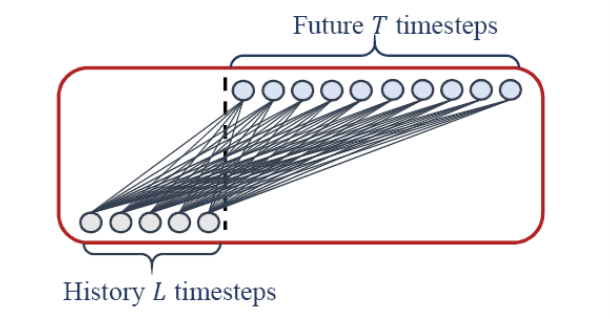
Figure 1: Architecture of LTSF-Linear.

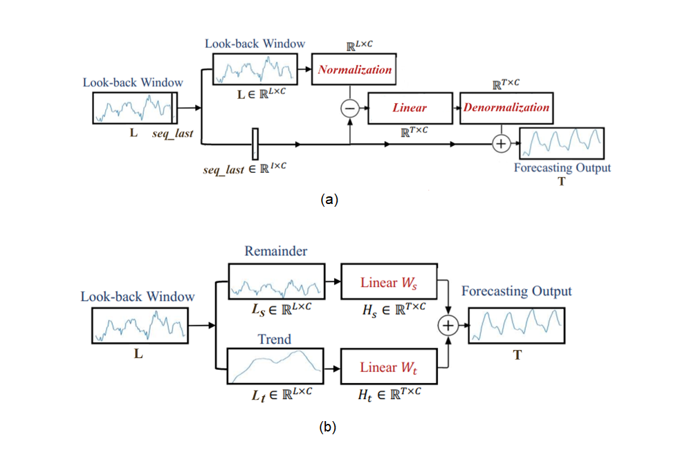
Figure 2: (a) The architecture of Nlinear predictor, (b) The architecture of DLinear predictor. The illustration of the architectures is created based on the description in the original paper [1].

III-A Linear Predictor (LTSF-Linear)

The first model is a LTSF-Linear predictor [1] where LTSF stands for long-term TSF. The architecture of the linear predictor can be visualized from Figure 1. This predictor is composed of a single fully connected linear layer, or dense layer. LSTF-Linear predictor does not model any spatial correlations. A single temporal linear layer directly regresses historical time series for future prediction via a weighted sum operation as follows:

$$T=WL+b$$ (1)

where $L$ refers to past input samples depending on defined input sequence length (can also be denoted as $X$), $T$ refers to predicted future samples depending on required prediction length (can also be denoted as $\hat{X}$), $W$ is weight matrix $W\in R^{T\times L}$ and $b$ is additive bias.

III-B NLinear Predictor (Normalization-based Linear Model)

To boost the performance of LTSF-Linear, NLinear [1] performs normalization to tackle the distribution shift in the dataset. NLinear first subtracts the input by the last value of the sequence, as shown in Figure 2 (a). Then, the input goes through a linear layer, and the subtracted part is added back before making the final prediction. The subtraction and addition in NLinear are a simple normalization for the input sequence.

III-C DLinear Predictor (Decomposition-based Linear Model)

DLinear [1] is a combination of a decomposition scheme used in Autoformer and FEDformer with linear layers. It first decomposes raw data input into a trend component by a moving average kernel and a remainder (seasonal) component as shown in Figure 2 (b). Then, two one-layer linear layers are applied to each component, and the two features are sum up to get the final prediction. By explicitly handling trend, DLinear enhances the performance of a vanilla linear when there is a clear trend in the data.

III-D RLinear Predictor (Reversible normalization-based Linear Model)

RLinear [2] combines a linear projection layer with RevIN to achieve competitive performance, as shown in Figure 3. The study reveals that RevIN enhances the model’s ability to handle distribution shifts and normalize input data effectively, leading to improved results even with a simpler architecture.

Figure 3: The schematic of the architecture of RLinear. The illustration of the architecture is created based on the description in the original paper [2].

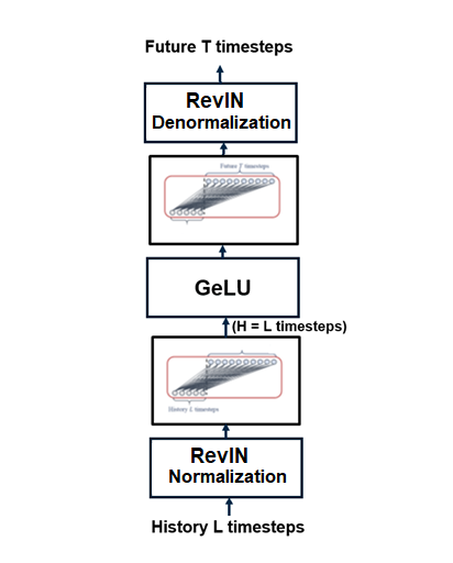
Figure 4: Architecture of the proposed GLinear predictor.

IV Methodology

Existing linear models use different simple operations like normalization and decomposition. It is worth noting that with the involvement of simpler mathematical operations, it is possible to build powerful linear predictors with some variations of activation functions to extract meaningful results for the required task [3]. Keeping these in mind, a new Gaussian-based linear predictor, GLinear, is proposed.

Figure 4 shows the architecture of the GLinear predictor that is composed of two fully-connected layers of the same input size having a GeLU nonlinearity in-between them. Different configurations of input and layers sizes are tested to lead to this final architecture. GeLU [5] is a non-linear activation function defined as follow:

$$\operatorname{GELU}(x)=x\cdot\Phi(x)$$ (2)

where $\Phi(x)$ refers to the cumulative distribution function (defined in (3)) of the standard normal distribution with an error function (erf).

$$\Phi(x)=\frac{1}{2}\left(1+\text{erf}\left(\frac{x}{\sqrt{2}}\right)\right)$$ (3)

Furthermore, RevIN is applied to the input and output layers of the GLinear model [4]. This normalization layer transforms the original data distribution into a mean-centred distribution, where the distribution discrepancy between different instances is reduced. This normalized data is then applied as new input to the used predictor, and then the final output is denormalized at the last step to provide the final prediction. RevIN can be used with any existing model. It does not add any significant overhead in training time due to low computational complexity of this normalization scheme.

The time-series data usually suffer from distribution shift problem due to changes in its mean and variance over time that can degrade the performance of time series predictors. RevIN utilizes learnable affine transformation to remove and restore the statistical information of a time-series instance that can be helpful to handle datasets with distribution shift problem.

Some features of GLinear model are:

• It is a simpler model; it is not made up of any complex components, functions or blocks (like self-attention schemes, positional encoding blocks, etc.). It integrates two components: (1) a non-linear GeLU-based transformation layer to capture intricate patterns, and (2) Reversible Instance Normalization (RevIN).

• Due to its simple architecture, training of this model is very fast as compared to other transformer based predictors.

• This proposed model provides comparable performance to other state-of-the-art predictors.

V Experimental Setup

In this section, we present the details about used datasets, experimental setup, and evaluation metrics.

V-A Dataset

We conducted experiments on four different real-world datasets (ETTh1, Electricity, Weather and Traffic). Table I provides a brief overview of these datasets.

V-A1 ETTh1

The ETTh1 dataset is used for long-sequence TSF in electric power. It includes two years of data from two Chinese counties, focusing on Electricity Transformer Temperature (ETT) [6]. It’s designed for detailed exploration of forecasting problems. This dataset is crucial for analyzing transformer temperatures and power load features in the electric power sector. ETTh1 differs from ETTh2 in granularity, focusing on long sequences compared to ETTh2’s hourly forecasting. The ETTh dataset serves the purpose of aiding research and analysis in the electric power sector, particularly for forecasting transformer temperatures and power load features. Applications of the ETTh dataset include research in long sequence time-series forecasting and studying power load features for better power deployment strategies.

The ETTh1 dataset is a multivariate time series dataset having 7 different variables (channels). It contains data of 725.83 days with granularity of 1 hour, meaning each timestamp represents a one-hour interval of data that provides 17420 timestamps values of each variable (17420 / 24 hours per day = 725.83 days of data).

V-A2 Electricity

The Electricity dataset [7] is also a multivariate time series dataset having 321 channels. It contains data of 1096 days with granularity of 1 hour that provides 26304 timestamps values of each channel (26304 / 24 hours per day = 1096 days of data).

V-A3 Weather

The Weather dataset [8] contains 52696 timestamp values collected in 365.86 days; each timestamp has 21 channels and a granularity of 10 minutes.

V-A4 Traffic

The Traffic dataset [9] contains 731 days of data with a granularity of 1 hour. It provides data of 862 channels each having 17544 timestamps values.

TABLE I: Overview of ETTh1, Electricity, Weather, and Traffic datasets.

Datasets	Timestamps	Variables(Channels)	Granularity
ETTh1	17420	7	1 hour
Electricity	26304	321	1 hour
Weather	52696	21	10 minutes
Traffic	17544	862	1 hour

V-B Implementation Details

The GLinear model is implemented using Python and is sourced from the official Pytorch implementation of LTSF-Linear . Respective code repository contains training and evaluation protocol of Autoformer, NLinear and DLinear. Similarly, the RLinear  model is trained and evaluated using the same protocol to ensure a fair comparison across all models.

The same set of hyperparameters are used for training all linear models, such as using the Mean Squared Error (MSE) criterion , Adam [11] optimizer and a learning rate of 0.001.

V-C Evaluation Metrics

The evaluation metrics used for comparison are MSE and Mean Absolute Error (MAE). These metrics are commonly used to assess the accuracy and performance of predictors [1, 12].

VI Experiments and Results

TABLE II: Multivariate Forecasting performance comparison across datasets and models (lower MSE/MAE is better). Input Sequence Length for all experiments is 336 and a range of Prediction Length {12, 24, 48, 96, 192, 336, 720} are used. The top-performing results are marked in bold. The second-best results are underlined.

		Lookup Window (Input Sequence Length) = 336 Learning Rate 0.001
Methods		Autoformer		NLinear		DLinear		RLinear		GLinear
Dataset / Output Horizon (Prediction Length)		MSE	MAE	MSE	MAE	MSE	MAE	MSE	MAE	MSE	MAE
Electricity	12	0.1638	0.2872	0.1000	0.2006	0.0997	0.2009	0.0967	0.1973	0.0883	0.1860
	24	0.1711	0.2917	0.1103	0.2092	0.1099	0.2089	0.1060	0.2049	0.0988	0.1952
	48	0.1827	0.2990	0.1255	0.2232	0.1249	0.2231	0.1201	0.2180	0.1144	0.2101
	96	0.1960	0.3106	0.1409	0.2366	0.1401	0.2374	0.1358	0.2317	0.1313	0.2258
	192	0.2064	0.3182	0.1551	0.2488	0.1538	0.2505	0.1518	0.2455	0.1494	0.2423
	336	0.2177	0.3290	0.1717	0.2654	0.1693	0.2678	0.1688	0.2621	0.1651	0.2582
	720	0.2477	0.3528	0.2104	0.2977	0.2042	0.3005	0.2071	0.2940	0.2027	0.2906
ETTh1	12	0.3991	0.4422	0.3069	0.3564	0.2976	0.3494	0.2862	0.3412	0.2848	0.3448
	24	0.4759	0.4733	0.3474	0.3842	0.3194	0.3627	0.3090	0.3559	0.3142	0.3654
	48	0.5046	0.4831	0.3553	0.3845	0.3477	0.3803	0.3454	0.3766	0.3537	0.3869
	96	0.5392	0.4979	0.3731	0.3941	0.3705	0.3919	0.3901	0.4054	0.3820	0.4025
	192	0.4907	0.4906	0.4089	0.4157	0.4044	0.4128	0.4223	0.4279	0.4202	0.4269
	336	0.4805	0.4886	0.4324	0.4307	0.4553	0.4582	0.4417	0.4383	0.4915	0.4715
	720	0.6303	0.5930	0.4369	0.4527	0.4975	0.5087	0.4634	0.4686	0.5923	0.5372
Traffic	12	0.5624	0.3830	0.3623	0.2662	0.3610	0.2644	0.3762	0.2744	0.3222	0.2385
	24	0.5801	0.3786	0.3719	0.2682	0.3709	0.2672	0.3834	0.2775	0.3369	0.2471
	48	0.6060	0.3796	0.3945	0.2769	0.3932	0.2760	0.4041	0.2864	0.3630	0.2607
	96	0.6426	0.3998	0.4113	0.2820	0.4104	0.2829	0.4194	0.2921	0.3875	0.2718
	192	0.6425	0.3967	0.4245	0.2872	0.4229	0.2881	0.4323	0.2965	0.4056	0.2802
	336	0.6675	0.4088	0.4375	0.2943	0.4362	0.2961	0.4451	0.3027	0.4200	0.2871
	720	0.6570	0.4030	0.4657	0.3109	0.4660	0.3152	0.4733	0.3191	0.4488	0.3038
Weather	12	0.2010	0.2933	0.0784	0.1127	0.0783	0.1158	0.0706	0.0974	0.0716	0.0940
	24	0.2095	0.3033	0.1056	0.1453	0.1040	0.1519	0.0905	0.1247	0.0909	0.1247
	48	0.2397	0.3202	0.1357	0.1824	0.1367	0.1937	0.1138	0.1566	0.1163	0.1602
	96	0.3004	0.3776	0.1761	0.2264	0.1756	0.2386	0.1450	0.1936	0.1457	0.1966
	192	0.3916	0.4382	0.2164	0.2595	0.2160	0.2739	0.1878	0.2339	0.1883	0.2385
	336	0.3830	0.4171	0.2664	0.2966	0.2652	0.3192	0.2404	0.2743	0.2407	0.2764
	720	0.5420	0.5032	0.3339	0.3437	0.3275	0.3667	0.3159	0.3271	0.3200	0.3334
Top 1 Performing		0		2		2		9		15
Top 2 Performing		0		5		10		17		23

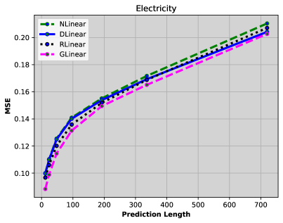
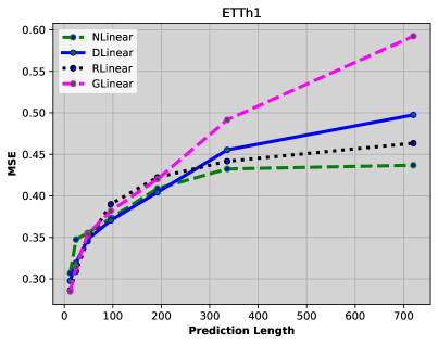
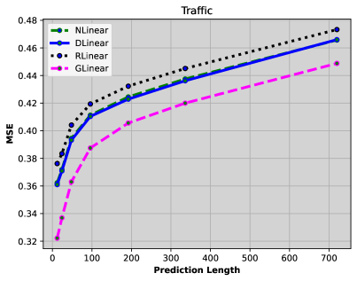
Figure 5: Multivariate Forecasting performance comparison across datasets and models. Input Sequence Length is 336 and values of Prediction Length are {12, 24, 48, 96, 192, 336, 720}. Datasets are (a) Electricity, (b) ETTh1, (c) Traffic, and (d) Weather.

The experimental setup was designed to assess GLinear’s performance in both short-term and long-term forecasting, as well as to analyze the impact of varying historical data lengths using two different experiments.

VI-A Evaluating Different Prediction Lengths for Fixed Input Length

In the first experiment, the length of the input sequence was fixed at 336 time steps, representing a historical window to learn the underlying patterns. The prediction lengths were varied across multiple time frames to assess the model’s ability to forecast different horizons, as displayed in Table II. Table II provides a comprehensive evaluation of all predictors, including Autoformer, NLinear, DLinear, RLinear, and the proposed GLinear across four datasets. In an extensive series of experiments, we varied the prediction lengths in range: {12, 24, 48, 96, 192, 336, 720}. This set of experiments allows for an evaluation of the model performance in forecasting short, medium and long-term future steps, helping to gauge the effectiveness of the model for various forecasting time horizons. We used a quantitative approach to score the best-performing candidate in all datasets, giving a point for the best and second-best results in each row. The results highlight that Glinear is a majority winner with substentially improved results in both evaluation metrics.

The performance of these models can also be compared using Figure 5. The results demonstrate that the proposed GLinear model outperforms other predictors in most cases (a lower MSE indicates better performance). Specifically, GLinear achieves the highest performance for the Electricity and Traffic datasets. For Weather forecasting, GLinear is the second-best model, with RLinear taking the top spot. However, the difference in MSE between the two models is minimal, as shown in Figure 5 (d). For the ETTh1 dataset, no single model consistently outperforms others across all prediction lengths. For the ETTh1 dataset, GLinear ranks among the top-performing models for shorter prediction lengths (12, 24, and 48), but the best-performing model changes as the prediction length increases. Additionally, the performance of GLinear deteriorates with longer prediction lengths for this dataset. The next experiment aims to provide an explanation to better understand the underlying reasons.

VI-B Impact of Input Sequence Length on Forecasting Future Steps

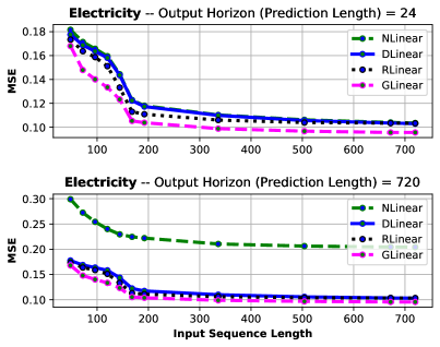
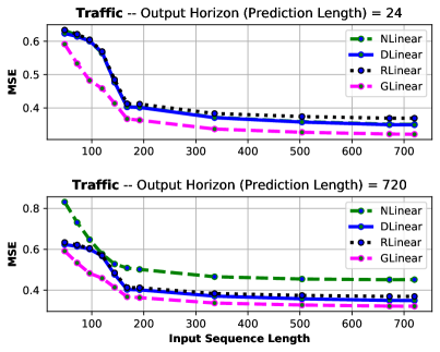
Figure 6: A performance comparison of all linear predictors (NLinear, DLinear, RLinear, and Proposed GLinear) with varying input sequence lengths in both long-term forecasting (720 time steps) and short-term forecasting (24 time steps) for different datasets, (a) Electricity, (b) ETTh1, (c) Traffic, and (d) Weather.

In the second experiment, the length of the input sequence was varied to understand how much historical data is required to accurately forecast the 24 and 720 future time steps. The input sequence lengths were set to {48, 72, 96, 120, 144, 168, 192, 336, 504, 672, 720}. For each of these input lengths, the model was trained to predict 24 and 720 future steps. This experiment aims to investigate how different lengths of historical data affect the model’s ability to generate accurate predictions for both short-term (24 steps) and long-term (720 steps) forecasts.

Figure 6 provides the result of the second experiment, which compares the performance of proposed GLinear with other state-of-the-art Linear predictors (NLinear, DLinear and RLinear) under different input prediction lengths to understand how much historical data is enough for short- and long-term forecasting. MSE results were computed for two prediction lengths (24 and 720 time steps) to analyze short-term and long-term forecasting performance, respectively.

It is worth noting that, similar to the previous experiment, the proposed GLinear model outperforms all other linear predictors for the Electricity and Traffic datasets. For the Weather dataset, both GLinear and RLinear show nearly identical forecasting performance.

The performance comparison of predictors on the ETTh1 dataset reveals interesting insights about the proposed GLinear model. Specifically, GLinear’s performance declines as it uses more historical data. However, it delivers the best performance for both short- and long-term forecasting when using shorter input sequence lengths, making it data-efficient by requiring less historical data to produce accurate forecasts.

VII Conclusion and Future Directions

In this paper, we have introduced GLinear, a novel and data-efficient architecture for multivariate time series forecasting (TSF) that leverages periodic patterns to enhance prediction accuracy while requiring less historical data compared to existing linear models. Our experiments across four datasets—ETTh1, Electricity, Traffic, and Weather—demonstrate that GLinear not only achieves competitive performance but also outperforms state-of-the-art models such as NLinear, DLinear, and RLinear, as well as Transformer-based models like Autoformer, in various TSF scenarios.

Overall, GLinear represents a promising step towards simpler, more efficient architectures for TSF tasks, achieving robust results with lower computational and data requirements. We believe that this approach opens new avenues for the development of efficient models for time series analysis, offering both better accuracy and computational savings.

Future work can explore applying the GLinear architecture to other time series-related tasks, such as anomaly detection or forecasting in different domains. Additionally, the periodic pattern extraction mechanism can be integrated into other deep learning models to enhance their efficiency and predictive performance.

Acknowledgment
This research has been partially funded by the European Union - Next Generation EU through the Project of National Relevance ”Innovative mathematical modeling for cell mechanics: global approach from micro-scale models to experimental validation integrated by reinforcement learning”, financed by European Union-Next-GenerationEU-National Recovery and Resilience Plan-NRRP-M4C1-I 1.1, CALL PRIN 2022 PNRR D.D. 1409 14-09-2022—(Project code P2022MXCJ2, CUP F53D23010080001) granted by the Italian MUR.

References

- [1] Zeng, A., Chen, M., Zhang, L. and Xu, Q., 2023, June. Are transformers effective for time series forecasting?. In Proceedings of the AAAI conference on artificial intelligence (Vol. 37, No. 9, pp. 11121-11128).
- [2] Li, Z., Qi, S., Li, Y. and Xu, Z., 2023. Revisiting long-term time series forecasting: An investigation on linear mapping. arXiv preprint arXiv:2305.10721.
- [3] Ni, R., Lin, Z., Wang, S. and Fanti, G., 2024, April. Mixture-of-Linear-Experts for Long-term Time Series Forecasting. In International Conference on Artificial Intelligence and Statistics (pp. 4672-4680). PMLR.
- [4] Kim, T., Kim, J., Tae, Y., Park, C., Choi, J.H. and Choo, J., 2021, May. Reversible instance normalization for accurate time-series forecasting against distribution shift. In International Conference on Learning Representations.
- [5] Hendrycks, D. and Gimpel, K., 2016. Gaussian error linear units (gelus). arXiv preprint arXiv:1606.08415.
- [6] Zhou, H., Zhang, S., Peng, J., Zhang, S., Li, J., Xiong, H. and Zhang, W., 2021, May. Informer: Beyond efficient transformer for long sequence time-series forecasting. In Proceedings of the AAAI conference on artificial intelligence (Vol. 35, No. 12, pp. 11106-11115).
- [7] Khan, Z.A., Hussain, T., Ullah, A., Rho, S., Lee, M. and Baik, S.W., 2020. Towards efficient electricity forecasting in residential and commercial buildings: A novel hybrid CNN with a LSTM-AE based framework. Sensors, 20(5), p.1399.
- [8] Angryk, R.A., Martens, P.C., Aydin, B., Kempton, D., Mahajan, S.S., Basodi, S., Ahmadzadeh, A., Cai, X., Filali Boubrahimi, S., Hamdi, S.M. and Schuh, M.A., 2020. Multivariate time series dataset for space weather data analytics. Scientific data, 7(1), p.227.
- [9] Chen, C., Petty, K., Skabardonis, A., Varaiya, P. and Jia, Z., 2001. Freeway performance measurement system: mining loop detector data. Transportation research record, 1748(1), pp.96-102.
- [10] Buansing, T. S. T., Golan, A., & Ullah, A. (2020). An information-theoretic approach for forecasting interval-valued SP500 daily returns. International Journal of Forecasting, 36(3), 800–813. Elsevier.
- [11] Kingma, D. P., & Ba, J. (2014). Adam: A method for stochastic optimization. arXiv.
- [12] Li, W., & Law, K. L. E. (2024). Deep learning models for time series forecasting: a review. IEEE Access. IEEE.
- [13] Makridakis, S., Spiliotis, E., & Assimakopoulos, V. (2018). Statistical and machine learning forecasting methods: Concerns and ways forward. PloS One, 13(3), e0194889. Public Library of Science
- [14] Kanwal, N., Eftestøl, T., Khoraminia, F., Zuiverloon, T. C. M., & Engan, K. (2023). Vision transformers for small histological datasets learned through knowledge distillation. In *Pacific-Asia Conference on Knowledge Discovery and Data Mining* (pp. 167–179). Springer.
- [15] Ariyo, A. A., Adewumi, A. O., & Ayo, C. K. (2014). Stock price prediction using the ARIMA model. In 2014 UKSim-AMSS 16th International Conference on Computer Modelling and Simulation (pp. 106–112). IEEE.
- [16] Abraham, G., Byrnes, G. B., & Bain, C. A. (2009). Short-term forecasting of emergency inpatient flow. IEEE Transactions on Information Technology in Biomedicine, 13(3), 380–388. IEEE.
- [17] Wazirali, R., Yaghoubi, E., Abujazar, M. S. S., Ahmad, R., & Vakili, A. H. (2023). State-of-the-art review on energy and load forecasting in microgrids using artificial neural networks, machine learning, and deep learning techniques. Electric Power Systems Research, 225, 109792. Elsevier.
- [18] Ouyang, T., He, Y., Li, H., Sun, Z., & Baek, S. (2019). Modeling and forecasting short-term power load with copula model and deep belief network. IEEE Transactions on Emerging Topics in Computational Intelligence, 3(2), 127–136. IEEE.
- [19] Zhou, S., Guo, S., Du, B., Huang, S., & Guo, J. (2022). A hybrid framework for multivariate time series forecasting of daily urban water demand using attention-based convolutional neural network and long short-term memory network. Sustainability, 14(17), 11086. MDPI.
- [20] Lin, Y., Koprinska, I., & Rana, M. (2021). Temporal convolutional attention neural networks for time series forecasting. In 2021 International Joint Conference on Neural Networks (IJCNN) (pp. 1–8). IEEE.
- [21] Dai, Z.-Q., Li, J., Cao, Y.-J., & Zhang, Y.-X. (2025). SALSTM: Segmented self-attention long short-term memory for long-term forecasting. The Journal of Supercomputing, 81(1), 115. Springer.
- [22] Tian, W., Luo, F., & Shen, K. (2024). PSRUNet: A recurrent neural network for spatiotemporal sequence forecasting based on parallel simple recurrent unit. Machine Vision and Applications, 35(3), 1–15. Springer.
- [23] Wu, N., Green, B., Ben, X., & O’Banion, S. (2020). Deep transformer models for time series forecasting: The influenza prevalence case. arXiv preprint arXiv:2001.08317.
- [24] Zhou, H., Zhang, S., Peng, J., Zhang, S., Li, J., Xiong, H., & Zhang, W. (2021, May). Informer: Beyond efficient transformer for long sequence time-series forecasting. In Proceedings of the AAAI conference on artificial intelligence (Vol. 35, No. 12, pp. 11106-11115).
- [25] Wu, H., Xu, J., Wang, J., & Long, M. (2021). Autoformer: Decomposition transformers with auto-correlation for long-term series forecasting. Advances in neural information processing systems, 34, 22419-22430.
- [26] Wu, H., Hu, T., Liu, Y., Zhou, H., Wang, J., & Long, M. (2022). Timesnet: Temporal 2d-variation modeling for general time series analysis. arXiv preprint arXiv:2210.02186.
- [27] Zhou, T., Ma, Z., Wen, Q., Wang, X., Sun, L., & Jin, R. (2022, June). Fedformer: Frequency enhanced decomposed transformer for long-term series forecasting. In International conference on machine learning (pp. 27268-27286). PMLR.
- [28] Li, D., Tan, Y., Zhang, Y., Miao, S., & He, S. (2023). Probabilistic forecasting method for mid-term hourly load time series based on an improved temporal fusion transformer model. International Journal of Electrical Power & Energy Systems, 146, 108743.
- [29] Aizpurua, J. I., Stewart, B. G., McArthur, S. D., Penalba, M., Barrenetxea, M., Muxika, E., & Ringwood, J. V. (2022). Probabilistic forecasting informed failure prognostics framework for improved RUL prediction under uncertainty: A transformer case study. Reliability Engineering & System Safety, 226, 108676.
- [30] Wang, H., Zou, D., Zhao, B., Yang, Y., Liu, J., Chai, N., & Song, X. (2024, June). RDLinear: A Novel Time Series Forecasting Model Based on Decomposition with RevIN. In 2024 International Joint Conference on Neural Networks (IJCNN) (pp. 1-7). IEEE.
- [31] O’Brien, C. M. (2016). Statistical learning with sparsity: the lasso and generalizations. Wiley Periodicals, Inc.
- [32] Ni, R., Lin, Z., Wang, S., & Fanti, G. (2024, April). Mixture-of-Linear-Experts for Long-term Time Series Forecasting. In International Conference on Artificial Intelligence and Statistics (pp. 4672-4680). PMLR.
- [33] Zhihao Zheng, V., Choi, S., & Sun, L. (2023). Enhancing Deep Traffic Forecasting Models with Dynamic Regression. arXiv e-prints, arXiv-2301.
- [34] Qayyum, H., Rizvi, S.T.H., Naeem, M., Khalid, U.B., Abbas, M. and Coronato, A., 2024. Enhancing Diagnostic Accuracy for Skin Cancer and COVID-19 Detection: A Comparative Study Using a Stacked Ensemble Method. Technologies, 12(9), p.142.
- [35] Kaur, J., Parmar, K. S., & Singh, S. (2023). Autoregressive models in environmental forecasting time series: a theoretical and application review. Environmental Science and Pollution Research, 30(8), 19617-19641.
- [36] Thu, N. T. H., Bao, P. Q., & Van, P. N. (2023). A hybrid model of decomposition, extended Kalman filter and autoregressive-long short-term memory network for hourly day ahead wind speed forecasting. J. Appl. Sci. Eng., 27, 3063-3071.