Bi-Parameterized Two-Stage Stochastic Min-Max and Min-Min Mixed Integer Programs

Abstract

We introduce two-stage stochastic min-max and min-min integer programs with bi-parameterized recourse (BTSPs), where the first-stage decisions affect both the objective function and the feasible region of the second-stage problem. To solve these programs efficiently, we introduce Lagrangian-integrated L-shaped ($L^{2}$) methods, which guarantee exact solutions when the first-stage decisions are pure binary. For mixed-binary first-stage programs, we present a regularization-augmented variant of this method. We also introduce distributionally robust bi-parameterized two-stage stochastic integer programs and present an extension of the $L^{2}$ method and a reformulation-based method for programs with finite and continuous supports, respectively. Our computational results show that the $L^{2}$ method surpasses the benchmark method for bi-parameterized stochastic network interdiction problems, solving all instances in 23 seconds on average, whereas the benchmark method failed to solve any instance within 3600 seconds. Additionally, it achieves optimal solutions up to 18.4 and 1.7 times faster for instances of risk-neutral and distributionally robust bi-parameterized stochastic facility location problems, respectively. Furthermore, BTSPs have applications in solving stochastic problems with decision-dependent probability distributions or sets of distributions (ambiguity set). The $L^{2}$ method outperforms existing approaches, achieving optimal solutions 5.3 times faster for distributionally robust facility location problem with a decision-dependent and non-relatively complete ambiguity set.

Key words:

Stochastic integer programs, Bi-parameterized recourse, Interdiction problems, Decision-dependent uncertainty, Distributionally robust optimization

1 Introduction

Two-stage stochastic programming is a well-known framework for modeling decision-making under uncertainty, where decisions are made sequentially over two stages: an initial set of (first-stage) decisions before the uncertainty is revealed, followed by a set of recourse (second-stage) decisions that adapt to revealed outcomes. This framework has been used for a wide variety of applications such as network interdiction (Smith and Song, 2020), healthcare (Yoon et al., 2021), power systems (Zheng et al., 2013, Zhang et al., 2020), airline crew scheduling (Yen and Birge, 2006), wildfire planning (Ntaimo et al., 2012), and many more (Luo et al., 2023, Sherali and Zhu, 2008, Üster and Memişoğlu, 2018). In this framework, it is typically assumed that the first-stage decisions affect only either the right-hand side (rhs) of the constraints or the objective function in the second-stage problem where the recourse decisions are made (Birge and Louveaux, 2011). In this paper, we investigate bi-parameterized two-stage stochastic programming, an extension of the conventional two-stage stochastic programming framework where the first-stage decisions affect the constraints and also the objective function of the second-stage problem. The formulation of bi-parameterized two-stage stochastic programs (BTSPs) is given by

$$\min_{x\in X}\Big{\{}f(x)+\mathbb{E}\big{[}Q(x,\tilde{\omega})\big{]}\Big{\}},$$ (1)

where vector $x$ denotes the set of first-stage decision variables, $\tilde{\omega}$ is a random variable with support $\Omega$, and for each realization $\omega\in\Omega$ of $\tilde{\omega}$, the recourse function $Q(x,\omega)$ is defined as follows:

$$Q(x,\omega):=\operatorname{min/max}\Big{\{}q(\omega)^{\top}y+x^{\top}G(\omega)y:W(\omega)y=r(\omega)-T(\omega)x,\ y\in\mathcal{Y}\Big{\}}.$$ (2)

The notation “$\operatorname{min/max}$” in (2) indicates that the recourse problem can either be a minimization problem or a maximization problem. Throughout the paper, we refer to BTSP 1 as min-min problem when the recourse problem 2 is a minimization, and min-max problem when the recourse problem is a maximization problem. It can be easily seen that this formulation reduces to the conventional “single-parameterized” two-stage stochastic program when $\operatorname{min/max}$ replaced with $\min$ and $G(\omega)=0$ for all $\omega\in\Omega$.

The first-stage feasible set is defined as $X:=\{x\in\mathcal{X}:Ax=b\}$, where $\mathcal{X}\subseteq\mathbb{R}^{n_{1}}_{+}$ represents integrality restrictions on $x$, $A\in\mathbb{Q}^{m_{1}\times n_{1}}$, and $b\in\mathbb{Q}^{m_{1}}$. The function $f:X\to\mathbb{R}$ is the first-stage objective function. Let $Y(x,\omega):=\{y\in\mathcal{Y}:W(\omega)y=r(\omega)-T(\omega)x\}$ for $\omega\in\Omega$ where $\mathcal{Y}\subseteq\mathbb{R}^{n_{2}}_{+}$ represents integrality restrictions on $y$. Here, $q(\omega)\in\mathbb{Q}^{n_{2}}$, $G(\omega)\in\mathbb{Q}^{n_{1}\times n_{2}}$, $T(\omega)\in\mathbb{Q}^{m_{2}\times n_{1}}$, $W(\omega)\in\mathbb{Q}^{m_{2}\times n_{2}}$, and $r(\omega)\in\mathbb{Q}^{m_{2}}$. Note that moving the parameterized term $x^{\top}G(\omega)y$ into the constraints using a proxy variable may result in a single-parameterized structure, where only constraints are parameterized by $x$. However, since the resulting constraints still depend on the parameterized coefficient, i.e., $x^{\top}G(\omega)$ for $y$, the problem structure differs from the conventional structure where coefficients associated with $y$ variables are independent on $x$.

The BTSPs pose computational challenges in solving due to the nonconvexity of their recourse functions, even without integrality restrictions on the second-stage variables $y$. To illustrate this, consider the following example:

Example 1.

Let $\Omega=\{\frac{1}{3},\frac{2}{3},1\}$ and $p(\omega)=1/3$ for $\omega\in\Omega$. Consider the following recourse function: $Q(x,\omega)=\min\{(1+x)y_{1}+(1+3x)y_{2}:y_{1}\geq x-\omega,\ y_{2}\geq\omega-x,\ y\in\mathbb{R}^{2}_{+}\},$ for $\omega\in\Omega$. The expected recourse function, i.e., $\mathbb{E}[Q(x,\tilde{\omega})]=\frac{1}{3}Q(x,\frac{1}{3})+\frac{1}{3}Q(x,\frac{2}{3})+\frac{1}{3}Q(x,1)$, on $[0,1]$ is nonconvex and nonsmooth, as illustrated in Figure 1.

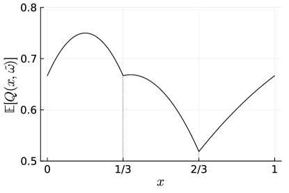
Figure 1: An example of a nonconvex expected recourse function.

$\blacksquare$

This complicates the application of Benders-type decomposition (or L-shaped method) to BTSPs, which relies on approximating the recourse function $Q(x,\omega)$ using valid (optimality) cuts. This method requires solving the second-stage subproblems that yields the subgradient to derive the valid cuts; however, obtaining the subgradient is not straightforward for BTSPs, due to the nonconvexity of the recourse function. The dual decomposition method (Carøe and Schultz, 1999) is another well-known approach for solving two-stage stochastic programs, particularly when the recourse problem involves integrality constraints. In this approach, copies of $x$, denoted by $x(\omega)$, are introduced and the nonanticipativity constraints, i.e., $x=x(\omega)$, for $\omega\in\Omega$ are relaxed. This allows for the scenario-wise decomposition of the problem. However, when applied to BTSPs, the dual decomposition method results in a mixed-integer nonconvex subproblem for each scenario, which could be computationally demanding to solve. In addition to nonconvexity, BTSPs present an additional challenge when the recourse problem includes integrality restrictions, thereby making the recourse function discontinuous as well.

Recently, smoothing-based approaches have been presented for the continuous case of the min-min problem 1 where $\mathcal{X}=\mathbb{R}^{n_{1}}_{+}$ and $\mathcal{Y}=\mathbb{R}^{n_{2}}_{+}$. Liu et al., (2020) propose an algorithm that converges almost surely to a generalized critical point. Their approach involves regularizing the recourse function, deriving a difference-of-convex decomposition of this regularized function, and then obtaining a convex upper-approximation. This allows them to update a solution $x$ by solving approximate problems using the convex approximation. For the convergence analysis, they identify an implicit convex-concave property of the recourse function $Q$. Li and Cui, (2024) also present a decomposition algorithm for two-stage stochastic programs with implicit convex-concave recourse functions where convex approximations of the recourse function are iteratively generated and solved, and the solutions converge to a critical point. Bomze et al., (2022) propose a bounding method for a class of bi-parameterized two-stage stochastic nonconvex programs where the objective function involves nonconvex quadratic terms and the feasible region is defined by a simplex. Note that none of the above approaches is directly applicable to BTSPs with integrality restrictions.

1.1 Applications of Bi-Parameterized Stochastic Programs

Many important classes of problems can be transformed into the BTSP formulation:

• Bi-parameterized network interdiction models. Network interdiction problems involve a sequential game between two players: an interdictor and a network user, with conflicting objectives. These problems have diverse applications in practice, such as disrupting illicit supply networks (Morton et al., 2007, Malaviya et al., 2012), planning military operation (Salmerón, 2012), and analyzing vulnerabilities in critical infrastructure (Brown et al., 2006). The formulation of stochastic network interdiction problems is given by the following min-max form:

  $$\min_{x\in X}\mathbb{E}\Big{[}\max_{y\in Y(x,\tilde{\omega})}f(x,y,\tilde{\omega})\Big{]},$$

  where $x$ denotes interdictor’s decision variables and $y$ represents network user’s decision variables. The function $f(x,y,\omega)$ and set $Y(x,\omega)$ for $\omega\in\Omega$ are the network user’s objective function and feasible set, respectively, and both of them depend on $x$. The formulation of bi-parameterized interdiction models has been considered a general form of interdiction problems in the literature (Smith and Song, 2020); however, to the best of our knowledge, no standard decomposition approaches have been established to address this general setup. We discuss further details of this application in Section 6.

• Stochastic optimization with decision-dependent uncertainty. Stochastic optimization often involves decision-dependent uncertainty, where a decision affects the distribution (for example, see (Dupacová, 2006, Hellemo et al., 2018)). Decision-dependent two-stage (risk-neutral) stochastic programs can be formulated as:

  $$\min_{x\in X}\Big{\{}f(x)+\mathbb{E}_{p(x)}\big{[}R(x,\tilde{\omega})\big{]}\Big{\}},$$

  where single-parameterized recourse function $R(x,\omega)=\min\{q(\omega)^{\top}y:W(\omega)y=r(\omega)-T(\omega)x,\ y\in\mathcal{Y}\}$ for $\omega\in\Omega$. Note that the expectation is taken with respect to the decision-dependent distribution $p(x)=(p(x,\omega))_{\omega\in\Omega}^{\top}$. By incorporating $p(x,\omega)$ into the objective function of each recourse problem $R(x,\omega)$, resulting in $(p(x,\omega)q(\omega)^{\top}y)$, the above formulation can be easily reformulated into the min-min problem 1.

  Furthermore, we can also consider a risk measure to model risk-averse behaviors of the decision-maker with the decision-dependent probabilities. For instance, decision-dependent two-stage risk-averse stochastic programs with conditional value-at-risk (CVaR) can be formulated as:

  $$\min_{x\in X}\Big{\{}f(x)+\operatorname{CVaR}_{\alpha}\big{(}R(x,\tilde{\omega}),p(x)\big{)}\Big{\}},$$

  where the CVaR is given by (Rockafellar and Uryasev, (2000)):

  $$\operatorname{CVaR}_{\alpha}(R(x,\tilde{\omega}),p(x))=$$ (3)

  $$\min_{\eta\in\mathbb{R}}\eta+\frac{1}{1-\alpha}\mathbb{E}_{p(x)}\Big{[}(R(x,\tilde{\omega})-\eta)_{+}\Big{]},$$

  which is a special case of the min-min problem 1. (Refer to Section 6 for details.)

• Distributionally robust optimization with decision-dependent ambiguity. Distributionally robust optimization (DRO) is an optimization framework that addresses uncertainty with distributional ambiguity, where the true distribution is unknown. In this framework, we consider a set of potential distributions, referred to as ambiguity set, that depends on the initial decision $x$; for example, see (Basciftci et al., 2021, Luo and Mehrotra, 2020, Yu and Shen, 2022, Kang and Bansal, 2024). Accordingly, a DRO model in this context can be formulated as:

  $$\min_{x\in X}\Big{\{}f(x)+\max_{p\in\mathcal{P}(x)}\mathbb{E}_{p}\big{[}R(x,\tilde{\omega})\big{]}\Big{\}},$$

  where $\mathcal{P}(x)$ is a decision-dependent ambiguity set and $R(x,\omega)$ is defined as above for $\omega\in\Omega$. The notation $\mathbb{E}_{p}$ represents the expectation with respect to distribution $p$. When the support $\Omega$ is finite, the ambiguity set $\mathcal{P}(x)$ is often defined by a polyhedron (e.g., Wasserstein ambiguity set, moment-matching ambiguity set, and $\phi$-divergence ambiguity set). In this case, by taking dual of the continuous relaxations of recourse (minimization) problems, we can derive a min-max (BTSP) reformulation of the DRO problem, which is a special case of the min-max problem 1. Refer to Section 6 for details.

  Non-Relatively Complete Ambiguity Set.

  A well-known method for this decision-dependent DRO problem is to dualize the inner maximization and reformulate the entire problem as a single minimization problem. This dual-based method, however, requires the ambiguity set $\mathcal{P}(x)$ to be nonempty for all $x\in X$, i.e., “relatively complete ambiguity set”. This assumption can be impractical, particularly when the ambiguity set is constructed to match the moment information of the new distribution with the empirical distribution of sample data; e.g., refer to Basciftci et al., (2021) and Yu and Shen, (2022). In Section 7.3, we demonstrate through numerical results that the dual-based approach fails to solve instances where $\mathcal{P}(x)$ is empty for some $x\in X$. We also show the method presented in this paper for BTSPs effectively addresses this issue, providing an exact solution to DRO problems without assuming the nonemptiness of $\mathcal{P}(x)$ for any $x\in X$.

1.2 Contributions and Organization of this Paper

In this paper, we introduce BTSPs, where integrality restrictions are involved in both the first and second stages. To efficiently solve these problems, we propose Lagrangian-integrated L-shaped ($L^{2}$) methods. Specifically, we present two exact algorithms for the min-max and min-min cases where the initial decision $x$ is pure binary, along with a regularization-augmented algorithm for the mixed-binary case. We also introduce extensions of the $L^{2}$ method to address DRO variants of BTSPs (DR-BTSPs) with finite or continuous support of random parameters. The numerical results demonstrate the efficiency of the $L^{2}$ methods. It solves all tested instances of network interdiction problems in 23 seconds on average, while the benchmark method fails to solve any instances within the time limit of 1 hour. Additionally, the $L^{2}$ method for min-min programs outperforms existing methods, achieving optimal solutions, on average, 18.4 and 1.7 times faster for risk-neutral and DR bi-parameterized stochastic facility location problems, respectively.

Furthermore, we show that many important problem classes can be efficiently solved by reformulating them as BTSP, including DRO with decision-dependent ambiguity and (risk-averse) stochastic optimization with decision-dependent uncertainty. Our approach can also effectively address DRO problems with decision-dependent ambiguity sets, even when these sets are not guaranteed to be nonempty for all initial decisions $x\in X$, which is a limitation of existing duality-based methods. For DRO problems with decision-dependent ambiguity sets, the $L^{2}$ method achieves the optimal solution, on average, 5.3 times faster than existing approaches.

Organization of the paper.

In section 2, we introduce an exact decomposition method for the min-max problem, and in section 3, we present its extension to solve the min-min problem. In section 4, we propose a regularization-augmented variant of our decomposition method. We introduce DR-BTSPs and algorithms to solve them in section 5, explore the applications of BTSPs in detail in section 6, and present computational results in section 7. In section 8, we make concluding remarks.

We make the following assumption on the feasible sets throughout the paper:

Assumption 1.

The set $X$ is nonempty and compact. Also, for all $x\in X$, the sets $Y(x,\omega)$ for $\omega\in\Omega$ are nonempty and compact.

Notation:

Let $[n]:=\{1,2,\dots,n\}$ for a positive integer $n$.

2 An exact algorithm for the min-max problem (1)

In this section, we introduce a decomposition method referred to as the Lagrangian-integrated L-shaped ($L^{2}$) method to exactly solve the min-max BTSP 1 with integer variables in both stages.

Lagrangian Relaxation.

By introducing proxy variables $z$ for $x$, we rewrite the recourse problem 2 as follows:

$$Q(x,\omega)=\max\ q(\omega)^{\top}y+x^{\top}G(\omega)y$$ (4a)

s.t. $$T(\omega)z+W(\omega)y=r(\omega),$$ (4b)

$$z=x,$$ (4c)

$$z\in X,\ y\in\mathcal{Y}.$$ (4d)

We relax constraints 4c with Lagrangian multipliers $\lambda(\omega)\in\mathbb{R}^{n_{1}}$. Then, the Lagrangian relaxation is given by $(L(x,\lambda(\omega),\omega)-\lambda(\omega)^{\top}x)$ where

$$L(x,\lambda(\omega),\omega)=\max\ q(\omega)^{\top}y+x^{\top}G(\omega)y+\lambda(\omega)^{\top}z$$ (5a)

s.t. $$T(\omega)z+W(\omega)y=r(\omega),z\in X,\ y\in\mathcal{Y}.$$ (5b)

For any $\lambda(\omega)\in\mathbb{R}^{n_{1}}$, the Lagrangian relaxation $(L(x,\lambda(\omega),\omega)-\lambda(\omega)^{\top}x)$ provides an upper bound on $Q(x,\omega)$. Therefore, the tightest upper bound is obtained by solving the following Lagrangian dual:

$$D(x,\omega):=\min_{\lambda(\omega)\in\mathbb{R}^{n_{1}}}\Big{\{}L(x,\lambda(\omega),\omega)-\lambda(\omega)^{\top}x\Big{\}}.$$ (6)

Assumption 2.

In the min-max problem 1, variables $x$ are mixed-integer and the components of $x$ that affect the recourse function $Q(x,\omega)$ are binary.

Theorem 1.

Under Assumption 2, $Q(x,\omega)=D(x,\omega)$ for any $\omega\in\Omega$ and $x\in X$, i.e., strong duality holds for the Lagrangian dual 6.

Proof.

Clearly, $Q(x,\omega)\leq D(x,\omega)$ for any $\omega\in\Omega$ and $x\in X$. Therefore, to prove the statement, it suffices to show that $Q(x,\omega)\geq D(x,\omega)$, for all $\omega\in\Omega$ and $x\in X$. Let $Z(\omega)$ for $\omega\in\Omega$ denote the feasible set of the Lagrangian relaxation 5. Also, we let $\tilde{T}(\omega)\in\mathbb{Q}^{\tilde{m}\times n_{1}},\tilde{W}(\omega)\in\mathbb{Q}^{\tilde{m}\times n_{2}},$ and $\tilde{r}(\omega)\in\mathbb{Q}^{\tilde{m}}$ such that $\operatorname{conv}(Z(\omega))=\{(y,z)\in\mathbb{R}^{n_{2}}_{+}\times\mathbb{R}^{n_{1}}_{+}:\tilde{T}(\omega)z+\tilde{W}(\omega)y\leq\tilde{r}(\omega)\}$. Then, we have

$$L(x,\lambda(\omega),\omega) =\max_{y\in\mathbb{R}^{n_{2}}_{+},z\in\mathbb{R}^{n_{1}}_{+}}\Big{\{}q(\omega)^{\top}y+x^{\top}G(\omega)y+\lambda(\omega)^{\top}z:\tilde{T}(\omega)z+\tilde{W}(\omega)y\leq\tilde{r}(\omega)\Big{\}}$$

$$=\min_{\pi\in\mathbb{R}^{\tilde{m}}_{+}}\Big{\{}\tilde{r}(\omega)^{\top}\pi:\tilde{T}(\omega)^{\top}\pi\geq\lambda(\omega),\tilde{W}(\omega)^{\top}\pi\geq q(\omega)+G(\omega)^{\top}x\Big{\}},$$

where $\pi$ are dual variables. By incorporating the above into the Lagrangian dual 6, we have

$$D(x,\omega)=\min_{\lambda(\omega)\in\mathbb{R}^{n_{1}},\pi\in\mathbb{R}^{\tilde{m}}_{+}}\Big{\{} \tilde{r}(\omega)^{\top}\pi-\lambda(\omega)^{\top}x:$$ (7)

$$\tilde{T}(\omega)^{\top}\pi-\lambda(\omega)\geq 0,\tilde{W}(\omega)^{\top}\pi\geq q(\omega)+G(\omega)^{\top}x\Big{\}}.$$

By taking dual of the above with multipliers $z\in\mathbb{R}_{+}^{n_{1}}$ and $y\in\mathbb{R}_{+}^{n_{2}}$ for the constraints, we have

$$\max_{y\in\mathbb{R}_{+}^{n_{2}},z\in\mathbb{R}_{+}^{n_{1}}}\Big{\{}q(\omega)^{\top}y+x^{\top}G(\omega)y:\tilde{T}(\omega)z+\tilde{W}(\omega)y\leq\tilde{r}(\omega),\ z=x\Big{\}}.$$ (8)

The feasible set of 8 is $\operatorname{conv}(Z(\omega))\cap\{(y,z):z=x\},$ which is a face of $\operatorname{conv}(Z(\omega))$ since $x$ is binary. By the facial property, any extreme point of this set has the $y$ components in $\mathcal{Y}$ and is feasible to the recourse problem 4, resulting in $D(x,\omega)\leq Q(x,\omega)$. ∎

Consequently, the min-max problem 1 can be exactly reformulated as

$$\min\bigg{\{}f(x)+\sum_{\omega\in\Omega}p(\omega)\Big{(}L(x,\lambda(\omega),\omega)-\lambda(\omega)^{\top}x\Big{)}:x\in X,\ \lambda(\omega)\in\mathbb{R}^{n_{1}},\ \forall\omega\in\Omega\bigg{\}}.$$ (9)

An advantage of addressing the reformulated problem instead of the original problem is that the Lagrangian function $L(\cdot,\cdot,\omega)$ for each $\omega\in\Omega$ is jointly convex on $\operatorname{conv}(X)\times\mathbb{R}^{n_{1}}$. This allows for the application of a decomposition method. Although the problem has the nonconvex terms with regard to $\lambda(\omega)^{\top}x$, we can employ convex approximations for these terms. However, the problem remains challenging due to the unboundedness of the Lagrangian multipliers $\lambda(\omega)$ which can lead to instability in updates when using cutting-plane or subgradient algorithms.

To address this challenge, we use an analytical form for the optimal Lagrangian multipliers.

Lemma 2.

There exist $\sigma_{i}\in\mathbb{R}_{+}$ for $i\in[n_{1}]$ such that, for any $\hat{x}\in X$, solution $\hat{\lambda}(\omega)=(\hat{\lambda}_{1}(\omega),\dots,\hat{\lambda}_{n_{1}}(\omega))$ where

$$\hat{\lambda}_{i}(\omega)=\begin{cases}-\sigma_{i}&\text{ if }\hat{x}_{i}=0\\ \sigma_{i}&\text{ if }\hat{x}_{i}=1\end{cases},\quad\text{for }i\in[n_{1}],\ \omega\in\Omega,$$ (10)

is an optimal solution to the Lagrangian dual 6.

Proof.

Given $(\hat{x},\hat{\lambda}(\omega))$, let $(\hat{y}(\omega),\hat{z}(\omega))$ be an optimal solution to the Lagrangian relaxation 5 for each $\omega\in\Omega$. There can be two cases: $\hat{z}(\omega)=\hat{x}$ and $\hat{z}(\omega)\neq\hat{x}$. Clearly, if $\hat{z}(\omega)=\hat{x}$, then $\hat{y}(\omega)$ is an optimal solution to the recourse problem, which implies that $\hat{\lambda}(\omega)$ is an optimal solution to the Lagrangian dual.

Now, consider the case where $\hat{z}(\omega)\neq\hat{x}$. Pick $\bar{y}(\omega)\in Y(\hat{x},\omega)$. Then, since solution $(y,z)=(\bar{y}(\omega),\hat{x})$ is non-optimal and feasible to the Lagrangian relaxation 5, we have

$$q(\omega)^{\top}\hat{y}(\omega)+\hat{x}^{\top}G(\omega)\hat{y}(\omega)+\hat{\lambda}(\omega)^{\top}\hat{z}(\omega)$$ (11)

$$>q(\omega)^{\top}\bar{y}(\omega)+\hat{x}^{\top}G(\omega)\bar{y}(\omega)+\hat{\lambda}(\omega)^{\top}\hat{x}.$$

By rearranging the terms, we obtain

$$(q(\omega)+G(\omega)^{\top}\hat{x})^{\top}(\hat{y}(\omega)-\bar{y}(\omega))>\hat{\lambda}(\omega)^{\top}(\hat{x}-\hat{z}(\omega))=\sum_{i\in I}\sigma_{i}$$ (12)

where $I:=\{i\in[n_{1}]:\hat{z}_{i}(\omega)\neq\hat{x}_{i}\}$. By Assumption 1, $\max_{y\in Y(\hat{x},\omega)}(q(\omega)+G(\omega)^{\top}\hat{x})^{\top}(\hat{y}(\omega)-y)<\infty$. This implies that there exist $\sigma_{i}\in\mathbb{R}_{+}$ for $i\in[n_{1}]$ such that the above inequality is violated for all $\bar{y}(\omega)\in Y(\hat{x},\omega)$. In other words, we can derive a sufficient condition under which it is enforced that $\hat{z}(\omega)=\hat{x}$ as follows:

$$\max_{y\in Y(\hat{x},\omega)}\Big{\{}(q(\omega)+G(\omega)^{\top}\hat{x})^{\top}(\hat{y}(\omega)-y)\Big{\}}\leq\sum_{i\in I}\sigma_{i}.$$ (13)

Hence, if $\sigma_{i}$ for $i\in[n_{1}]$ satisfy the condition 13 for all $\hat{x}\in X$, then, for any $\hat{x}\in X$, solutions $\hat{\lambda}(\omega)$ for $\omega\in\Omega$ are optimal to the Lagrangian duals. ∎

Remark 1.

To find a vector $\sigma\in\mathbb{R}^{n_{1}}_{+}$ that satisfies condition 13 for all $\hat{x}\in X$, we can use known upper and lower bounds on the objective value 1. Since their difference is always greater than or equal to the left-hand side (lhs) of 13, setting $\sigma_{i}(\omega)$ to the difference for $i\in[n_{1}]$ and $\omega\in\Omega$ ensures that $\sigma(\omega)$ satisfies condition 13. An alternate method is to solve an optimization problem to get $\sigma$. For example, let $\Delta_{y}(x,\omega)=\{y^{1}-y^{2}:y^{1},y^{2}\in Y(x,\omega)\}$ and consider $\sigma_{i}(\omega)=\max\big{\{}\big{(}\frac{q(\omega)}{n_{1}}+G_{i}(\omega)x_{i}\big{)}^{\top}\delta_{y}:x\in X,\ \delta_{y}\in\Delta_{y}(x,\omega)\big{\}}$ for $i\in[n_{1}]$ and $\omega\in\Omega$. Here, $G_{i}(\omega)$ is the $i$th column of $G(\omega)$. These problems can be reformulated as mixed-integer linear programs by adding McCormick inequalities to linearize the bilinear terms $x_{i}\delta_{y}$. The $\sigma_{i}(\omega)$ values satisfy the condition 13 as $\sum_{i\in[n_{1}]}\sigma_{i}(\omega)=\sum_{i\in[n_{1}]}\max\big{\{}\big{(}\frac{q(\omega)}{n_{1}}+G_{i}(\omega)x_{i}\big{)}^{\top}\delta_{y}:x\in X,\ \delta_{y}\in\Delta_{y}(x,\omega)\big{\}}\geq\max\{(q(\omega)+G(\omega)^{\top}x)^{\top}\delta_{y}:x\in X,\ \delta_{y}\in\Delta_{y}(x,\omega)\}$ for $\omega\in\Omega$. The inequality holds since an optimal solution to the rhs problem is feasible to the problem on the lhs for each $i\in[n_{1}]$.

Theorem 3.

There exists vector $\sigma=(\sigma_{1},\dots,\sigma_{n_{1}})\in\mathbb{R}^{n_{1}}_{+}$ such that the following problem is an exact reformulation of the min-max problem 1:

$$\min_{x\in X}\Big{\{}f(x)-\sigma^{\top}x+\sum_{\omega\in\Omega}p(\omega)\hat{Q}(x,\omega)\Big{\}}$$ (14)

where, for each $\omega\in\Omega$,

$$\hat{Q}(x,\omega)=\max q(\omega)^{\top}y+x^{\top}G(\omega)y+\sum_{i\in[n_{1}]}\sigma_{i}(2x_{i}-1)z_{i}$$ (15)

s.t. $$T(\omega)z+W(\omega)y=r(\omega),\ z\in X,\ y\in\mathcal{Y}.$$

Proof.

Let vector $\sigma=(\sigma_{1},\dots,\sigma_{n_{1}})\in\mathbb{R}^{n_{1}}_{+}$ satisfies the condition 13 for all $\omega\in\Omega$ and $\hat{x}\in X$. Then according to lemma 2, in the reformulation 9, we can fix $\lambda(\omega)$ to its optimal value using the analytical form: $\lambda_{i}(\omega)=\sigma_{i}(2x_{i}-1),i\in[n_{1}]$, for $\omega\in\Omega$. Consequently, we can substitute the bilinear terms $\lambda(\omega)^{\top}x$ and $\lambda(\omega)^{\top}z$ in the objective functions as follows: $\lambda(\omega)^{\top}x=\sum_{i=1}^{n_{1}}\sigma_{i}(2x_{i}-1)x_{i}=\sigma^{\top}x,$ and $\lambda(\omega)^{\top}z=\sum_{i=1}^{n_{1}}\sigma_{i}(2x_{i}-1)z_{i}$ for $\omega\in\Omega$. This results in the formulation 14. ∎

1 Initialization: $l\leftarrow 1,LB\leftarrow-\infty,UB\leftarrow\infty,x^{1}\in X$;

2 while $(UB-LB)/UB>\varepsilon^{tol}$ do

3    Solve the subproblems, obtain $\{(y^{l}(\omega),z^{l}(\omega))\}_{\omega\in\Omega}$, and compute $\hat{Q}(x^{l},\omega)$;

4    Compute $\phi^{l}=f(x^{l})-\sigma^{\top}x^{l}+\sum_{\omega\in\Omega}p(\omega)\hat{Q}(x^{l},\omega)$;

5    if $\phi^{l}<UB$ then

6       $UB\leftarrow\phi^{l}$; $x^{\ast}\leftarrow x^{l}$;

7      

8   Add an optimality cut to master problem;

9    Solve the master problem and obtain optimal solution $(x^{l+1},\hat{\theta})$;

10    $LB\leftarrow f(x^{l+1})-\sigma^{\top}x^{l+1}+\hat{\theta}$;

11    $l\leftarrow l+1$;

12   

13return $x^{\ast}$;

Algorithm 1 The $L^{2}$ method for the min-max problem

Lagrangian-Integrated L-Shaped Method.

We now present the $L^{2}$ method for solving the min-max problem 1 through its reformulation 14. At each iteration, the $L^{2}$ method adds a valid cut, referred to as optimality cut, that approximates the function $\sum_{\omega\in\Omega}p(\omega)\hat{Q}(x,\omega)$ in 14. The pseudo-code of the $L^{2}$ method is outlined in Algorithm 1. It starts by initializing iteration counter $l$ to $1$, lower bound $LB$ to $-\infty$, and upper bound $UB$ to $\infty$. Let $x^{1}\in X$ be any feasible solution. For each iteration $l$, we first solve the subproblems for $\omega\in\Omega$, which is given by the formulation 15 with $x=x^{l}$. Subsequently, we compute the objective value at the current solution $x^{l}$, denoted by $\phi^{l}$. If this value $\phi^{l}$ is less than the current upper bound $UB$, then it replaces $UB$, and the current solution is saved as the best-known solution. Next, using the optimal solutions to the subproblems, an optimality cut is obtained and then added to the master problem. In iteration $l$, master problem is given as follows:

$$\min\ \bigg{\{} f(x)-\sigma^{\top}x+\theta:x\in X,$$ (16)

$$\theta\geq\sum_{\omega\in\Omega}p(\omega)\Big{(}q(\omega)^{\top}y^{k}(\omega)+x^{\top}G(\omega)y^{k}(\omega)+\sum_{i\in[n_{1}]}\sigma_{i}(2x_{i}-1)z^{k}_{i}(\omega)\Big{)},\ \forall k\in[l]\bigg{\}},$$

where $(y^{k}(\omega),z^{k}(\omega))_{k\in[l]}$ are the optimal solutions of the subproblems at the corresponding iterations. In the following step, we solve the master problem, obtain a first-stage solution $x^{l+1}$ to be explored in the next iteration, and replace the lower bound $LB$ with the objective value of the master problem. We repeat this procedure until the optimality gap is less than or equal to a predetermined tolerance level $\varepsilon^{tol}$.

Proposition 4.

Let vector $\sigma\in\mathbb{R}^{n_{1}}_{+}$ satisfies the condition 13 for all $\omega\in\Omega$ and $x\in X$, and let $\varepsilon^{tol}=0$. Under Assumption 2, Algorithm 1 terminates in a finite number of iterations with $x^{\ast}$ optimal to the min-max BTSP 1.

Proof.

Let $\phi(x)$ be the objective function of the reformulation 14. To prove the statement, it suffices to show that Algorithm 1 terminates with $UB=LB$ in a finite number of iterations, as this implies that $\phi(x^{\ast})=UB=LB\leq\min_{x\in X}\phi(x)=\min_{x\in X}\{f(x)+\sum_{\omega\in\Omega}p(\omega)Q(x,\omega)\}$. The last equality holds by Theorem 3.

For a solution $(y^{l}(\omega),z^{l}(\omega))$ and $\omega\in\Omega$, we have $\hat{Q}(x,\omega)\geq q(\omega)^{\top}y^{l}(\omega)+x^{\top}G(\omega)y^{l}(\omega)+\sum_{i\in[n_{1}]}\sigma_{i}(2x_{i}-1)z^{l}_{i}(\omega)$ since the solution is feasible to the problem 15. Furthermore, the inequality is tight at $x^{l}$, i.e., $\hat{Q}(x^{l},\omega)=q(\omega)^{\top}y^{l}(\omega)+(x^{l})^{\top}G(\omega)y^{l}(\omega)+\sum_{i\in[n_{1}]}\sigma_{i}(2x_{i}^{l}-1)z^{l}_{i}(\omega)$. Thus, the optimality cut generated using solutions $(y^{l}(\omega),z^{l}(\omega)),\omega\in\Omega,$ for iteration $l$ is a valid cut that supports the epigraph of $\sum_{\omega\in\Omega}p(\omega)\hat{Q}(x,\omega)$ at $x^{l}$, thus ensuring that the master problem exactly evaluates the objective value in the incumbent solution $x^{l}$. Since $|X|<\infty$, there exists $l<\infty$ such that $\hat{\theta}=\sum_{\omega\in\Omega}p(\omega)\hat{Q}(x^{l+1},\omega)$ at Algorithm 1. This implies that $UB=LB$, as $x^{l+1}$ is feasible to the original reformulation 14. ∎

Remark 2.

To accelerate Algorithm 1, we can fix $z$ to $x^{l}$ when solving the subproblem in Algorithm 1. Solving this restricted subproblem with $z=x^{l}$ yields a feasible solution to the original problem 15, allowing us to derive an optimality cut valid for $\hat{Q}(x,\omega)$. This approach reduces computational effort while still providing a valid cut.

3 An exact algorithm for the min-min problem (1)

The $L^{2}$ method for the min-min problem 1 begins by deriving its min-max reformulation. To this end, we convexify the recourse feasible region $Y(x,\omega)$, which is achieved sequentially by adding parametric inequalities. We make the following assumption for the exactness of our algorithm.

Assumption 3.

In the min-min problem, all first-stage variables $x$ are binary, i.e., $\mathcal{X}=\{0,1\}^{n_{1}}.$

Let $S(\omega):=\{(x,y)\in X\times\mathcal{Y}:T(\omega)x+W(\omega)y=r(\omega)\}$ be a lifted feasible set in the $(x,y)$-space for $\omega\in\Omega$. Assume that $\tilde{T}(\omega)\in\mathbb{Q}^{m(\omega)\times n_{1}},\tilde{W}(\omega)\in\mathbb{Q}^{m(\omega)\times n_{2}},$ and $\tilde{r}(\omega)\in\mathbb{Q}^{m(\omega)}$ appropriately sized matrices and vectors such that $\operatorname{conv}(S(\omega))=\{(x,y)\in\mathbb{R}^{n_{1}}_{+}\times\mathbb{R}^{n_{2}}_{+}:\tilde{T}(\omega)x+\tilde{W}(\omega)y\geq\tilde{r}(\omega)\}$. The intersection of $\operatorname{conv}(S(\omega))$ and the hyperplane $\{(x,y):x=\hat{x}\}$ for any $\hat{x}\in X$ is a face of $S(\omega)$, as $x$ is binary, thereby all extreme points in the intersection have the $y$ components in $\mathcal{Y}$. By this observation, for any $\hat{x}\in X$, we have

$$Q(\hat{x},\omega) =\min\bigg{\{}q(\omega)^{\top}y+\hat{x}^{\top}G(\omega)y:(x,y)\in\operatorname{conv}(S(\omega))\cap\Big{\{}(x,y):x=\hat{x}\Big{\}}\bigg{\}}$$ (17)

$$=\min\bigg{\{}q(\omega)^{\top}y+\hat{x}^{\top}G(\omega)y:\tilde{W}(\omega)y\geq\tilde{r}(\omega)-\tilde{T}(\omega)\hat{x},\ y\in\mathbb{R}^{n_{2}}_{+}\bigg{\}}.$$ (18)

Without loss of generality, we can assume $m(\omega)$ is finite since $Y(x,\omega)$ is bounded. That is, the convex hull $\operatorname{conv}(S(\omega))$ can be represented with finitely many parametric inequalities in the form of $(\alpha^{1})^{\top}x+(\alpha^{2})^{\top}y\geq\beta$; e.g., lift-and-project cuts (Balas et al., 1993) and Gomory cuts (Gomory, 1963). Thus, the linear programming dual of 18 is given by

$$Q(x,\omega)=\max\bigg{\{}\pi^{\top}(\tilde{r}(\omega)-\tilde{T}(\omega)x):\tilde{W}(\omega)^{\top}\pi\leq q(\omega)+G(\omega)^{\top}x,\ \pi\in\mathbb{R}_{+}^{m(\omega)}\bigg{\}}.$$ (19)

Then, we can rewrite the min-min problem as the following min-max problem:

$$\min_{x\in X}\bigg{\{}f(x)+\sum_{\omega\in\Omega}p(\omega)\max\Big{\{} \pi^{\top}(\tilde{r}(\omega)-\tilde{T}(\omega)x):$$ (20)

$$\tilde{W}(\omega)^{\top}\pi\leq q(\omega)+G(\omega)^{\top}x,\ \pi\in\mathbb{R}_{+}^{m(\omega)}\Big{\}}\bigg{\}}.$$

By applying the result in Theorem 3 to the above min-max reformulation, we obtain the following another reformulation of the min-min problem: $\min_{x\in X}f(x)-\sigma^{\top}x+\sum_{\omega\in\Omega}p(\omega)\hat{Q}(x,\omega)$ where

$$\hat{Q}(x,\omega)=\max\ \pi^{\top}(\tilde{r}(\omega)-\tilde{T}(\omega)x)+\sum_{i\in[n_{1}]}\sigma_{i}(2x_{i}-1)z_{i}$$ (21a)

s.t. $$\tilde{W}(\omega)^{\top}\pi-G(\omega)^{\top}z\leq q(\omega)$$ (21b)

$$z\in X,\ \pi\in\mathbb{R}^{m(\omega)}_{+}.$$ (21c)

Now we present the $L^{2}$ method for the min-min problem. Its pseudo-code is outlined in Algorithm 2. The algorithm sequentially convexifies the set $S(\omega)$, i.e., it constructs the information $\{\tilde{T}(\omega),\tilde{W}(\omega),\tilde{r}(\omega)\}_{\omega\in\Omega}$ by adding parametric inequalities to subproblems. To this end, we consider an oracle that provides a violated parametric inequality if there exists any, which is the cut-generating linear program presented in Balas et al., (1993). We refer to such an oracle as the cut-generating oracle.

1 Initialization: $l\leftarrow 1,LB\leftarrow-\infty,UB\leftarrow\infty,x^{1}\in X$;

2 while $(UB-LB)/UB>\varepsilon^{tol}$ do

3    for $\omega\in\Omega$ do

4       Solve the primal subproblem and obtain optimal solution $y^{l}(\omega)$;

5       if $y^{l}(\omega)\notin\mathcal{Y}$ then

6          Find a violated parametric inequality using the cut-generating oracle;

7          $(T^{l}(\omega),W^{l}(\omega),r^{l}(\omega))\leftarrow(T^{l-1}(\omega),W^{l-1}(\omega),r^{l-1}(\omega))$ appended with the information of the parametric inequality;

8         

9      else

10          $(T^{l}(\omega),W^{l}(\omega),r^{l}(\omega))\leftarrow(T^{l-1}(\omega),W^{l-1}(\omega),r^{l-1}(\omega))$;

11         

12      

13   Solve the dual subproblems, obtain $\{(\pi^{l}(\omega),z^{l}(\omega))\}_{\omega\in\Omega}$, and compute $\hat{Q}^{l}(x^{l},\omega)$;

14   

15   Compute $\psi^{l}=f(x^{l})-\sigma^{\top}x^{l}+\sum_{\omega\in\Omega}p(\omega)\hat{Q}^{l}(x^{l},\omega)$;

16    if $y^{l}(\omega)\in\mathcal{Y},\forall\omega\in\Omega$ and $\psi^{l}<UB$ then

17       $UB\leftarrow\psi^{l}$; $x^{\ast}\leftarrow x^{l}$;

18      

19   Add an optimality cut to master problem;

20    Solve the master problem and obtain optimal solution $(x^{l+1},\hat{\theta})$;

21    $LB\leftarrow f(x^{l+1})-\sigma^{\top}x^{l+1}+\hat{\theta}$;

22    $l\leftarrow l+1$;

23   

24return $x^{\ast}$;

Algorithm 2 The $L^{2}$ method for the min-min problem

Algorithm 2 starts by initializing iteration counter $l$ to 1, lower bound $LB$ to $-\infty$, and upper bound $UB$ to $\infty$. Let $x^{1}\in X$ be any feasible solution. At each iteration $l$, we first solve the following problems, called primal subproblems:

$$\min\Big{\{}q(\omega)^{\top}y+(x^{l})^{\top}G(\omega)y:W^{l-1}(\omega)y\geq r^{l-1}(\omega)-T^{l-1}(\omega)x^{l},\ y\in\mathbb{R}^{n_{2}}_{+}\Big{\}},$$ (22)

where $(T^{0}(\omega),W^{0}(\omega),r^{0}(\omega))=(T(\omega),W(\omega),r(\omega))$, for $\omega\in\Omega$. The matrices and vector are updated to $(T^{l}(\omega),W^{l}(\omega),r^{l}(\omega))$ through the following procedure. Let $y^{l}(\omega)$ be the optimal solution to the primal subproblems for $\omega\in\Omega$. If $y^{l}(\omega)\notin\mathcal{Y}$, then the cut-generating oracle is used, and a violated parametric inequality is added to the primal subproblem. Otherwise, we keep the current matrices and vector. Notice that the primal subproblem is a relaxation of the recourse problem 18, thereby through this approach the $L^{2}$ method refines the relaxation iteratively. In the next step, we solve the following problems for $\omega\in\Omega$, referred to as dual subproblems:

$$\hat{Q}^{l}(x^{l},\omega)=\max\Big{\{} \pi^{\top}(r^{l}(\omega)-T^{l}(\omega)x^{l})+\sum_{i\in[n_{1}]}\sigma_{i}(2x^{l}_{i}-1)z_{i}:$$ (23)

$$W^{l}(\omega)^{\top}\pi-G(\omega)^{\top}z\leq q(\omega),\ z\in X,\ \pi\in\mathbb{R}^{m^{l}}_{+}\Big{\}}.$$

where $\sigma$ is a given vector that satisfies the condition 13 for all $\omega\in\Omega$ and $x\in X$. Note that the dimension $m^{l}$ of variables $\pi$ varies over iterations corresponding to the updates in the information $(T^{l}(\omega),W^{l}(\omega),r^{l}(\omega))$. After solving the dual subproblems, an under-approximation $\psi^{l}$ of the objective value at the current solution $x^{l}$ is computed; this objective value is exact if $y^{l}(\omega)\in\mathcal{Y}$ for all $\omega\in\Omega$. If $\psi^{l}$ is exact and $\psi^{l}<UB$, then we update the upper bound, and the current solution is marked as the best solution so far. Subsequently, using the optimal solutions of the dual subproblems, an optimality cut is computed and added to master problem that is given by

$$\min\bigg{\{} f(x)-\sigma^{\top}x+\theta:x\in X,$$ (24a)

$$\theta\geq\sum_{\omega\in\Omega}p(\omega)\Big{(}\pi^{k}(\omega)^{\top}(r^{k}(\omega)-T^{k}(\omega)x)+\sum_{i\in[n_{1}]}\sigma_{i}z_{i}^{k}(\omega)(2x_{i}-1)\Big{)},\ \forall k\in[l]\bigg{\}}.$$ (24b)

Constraints 24b are optimality cuts added for iteration $k\in[l]$ where $(\pi^{k}(\omega),z^{k}(\omega))_{k\in[l]}$ are optimal solutions of the dual subproblems at the corresponding iterations.

Proposition 5.

The optimality cut obtained at iteration $l$ is valid for $\sum_{\omega\in\Omega}p(\omega)\hat{Q}(x,\omega)$, i.e., $\sum_{\omega\in\Omega}p(\omega)\hat{Q}(x,\omega)\geq\sum_{\omega\in\Omega}p(\omega)\Big{(}\pi^{l}(\omega)^{\top}(r^{l}(\omega)-T^{l}(\omega)x)+\sum_{i\in[n_{1}]}\sigma_{i}z_{i}^{l}(\omega)(2x_{i}-1)\Big{)}$.

Proof.

For scenario $\omega$ and iteration $l$, the dual subproblem can be viewed as a restriction of the reformulated recourse problem 21 where variables $\pi_{k}$ for $k=m^{l}+1,\dots,m(\omega)$ are restricted to be zero. Let $(\hat{\pi}(\omega),z^{l}(\omega))$ be a lifted solution of $(\pi^{l}(\omega),z^{l}(\omega))$, where $\hat{\pi}_{k}(\omega)=\pi^{l}_{k}(\omega)$ for $k=1,\dots,m(\omega)$ and $\hat{\pi}_{k}(\omega)=0$ for $k=m^{l}+1,\dots,m(\omega)$. This solution is feasible to problem 21, and thus the following inequality holds:

$$\hat{Q}(x,\omega) \geq\hat{\pi}(\omega)^{\top}(\tilde{r}(\omega)-\tilde{T}(\omega)x)+\sum_{i\in[n_{1}]}\sigma_{i}z^{l}_{i}(\omega)(2x_{i}-1)$$

$$=\pi^{l}(\omega)^{\top}(r^{l}(\omega)-T^{l}(\omega)x)+\sum_{i\in[n_{1}]}\sigma_{i}z^{l}_{i}(\omega)(2x_{i}-1).$$

Multiplying the inequality by $p(\omega)$ and summing over all $\omega\in\Omega$ yields the optimality cut. ∎

Next, we solve the master problem and obtain a new lower bound on the optimal objective value. It also identifies a solution $x^{l+1}$ to be explored in the next iteration. This process is repeated until the optimality gap, $(UB-LB)/UB$, equals or falls below a predetermined tolerance level $\varepsilon^{tol}\geq 0$.

4 A regularization-augmented algorithm for BTSPs

Algorithms 1 and 2 rely on a specific $\sigma$ that satisfies the condition in 13, which is required for their exactness, under the binary assumption on the first-stage decisions $x$. In this section, we propose an alternative approach that does not require a predetermined $\sigma$ and can handle mixed-binary $x$ in BTSPs. Specifically, this approach directly addresses the Lagrangian reformulation of BTSPs 9. For simplicity, we focus on the min-max problem, yet the approach in this section can be applied to the min-min problem similarly. Therefore, the functions $L(x,\lambda(\omega),\omega)$ for $\omega\in\Omega$ are given by 5.

We first address the instability of the Lagrangian multipliers. Specifically, we investigate the instability that arises when updating the Lagrangian multipliers within a cutting-plane algorithm for the above problem. Subsequently, we show how this issue can be resolved through a reformulation.

Recall that the multipliers $\lambda(\omega)$ represent the penalties associated with the difference between $z$ and $x$ in scenario $\omega$. As shown in Lemma 2, when $x\in\{0,1\}^{n_{1}}$, an optimal penalty can be expressed as $\hat{\lambda}_{i}(\omega)=\sigma_{i}(2x_{i}-1),i\in[n_{1}]$ for sufficiently large $\sigma\in\mathbb{R}^{n_{1}}_{+}$. This implies that a change in $x$ can result in a significant change in the corresponding values of the multipliers. For example, if $x_{i}$ changes from $0$ to $1$, then the optimal value for $\lambda_{i}(\omega)$ changes from $-\sigma_{i}$ to $\sigma_{i}$. Consequently, when $x$ is updated at each iteration of the cutting-plane algorithm, significant adjustments to the Lagrangian multipliers may be required, causing unstable convergence.

To mitigate this instability, we derive an alternative formulation where the updates focus on the absolute values of the Lagrangian multipliers. Consider arbitrary upper bounds $\bar{u}\in\mathbb{R}^{n_{1}}_{+}$ on the absolute values of the optimal multipliers. We can rewrite the problem 9 as follows:

$$\min_{x\in X}\ f(x)+\sum_{\omega\in\Omega}p(\omega)\Big{(}L(x,\lambda(\omega),\omega)-\lambda(\omega)^{\top}x\Big{)}$$ (25a)

s.t. $$-\bar{u}\leq\lambda(\omega)\leq\bar{u},\quad\forall\omega\in\Omega.$$ (25b)

We introduce variables $\mu(\omega)\in\mathbb{R}^{n_{1}}$ for $\omega\in\Omega$ to represent the absolute values of the multipliers $\lambda(\omega)$. Under Assumptions 2 and 3, there exists an optimal $\lambda_{i}(\omega)$ that is nonnegative when $x_{i}=1$ and nonpositive when $x_{i}=0$. Based on this observation, we express $\lambda_{i}(\omega)$ as $\mu_{i}(\omega)(2x_{i}-1)$ for each $i\in[n_{1}]$. Consequently, the problem can be reformulated as follows:

$$\min_{x\in X}\ f(x)+\sum_{\omega\in\Omega}p(\omega)\Big{(}L(x,\lambda(\omega),\omega)-\mu(\omega)^{\top}x\Big{)}$$ (26a)

s.t. $$\lambda_{i}(\omega)=\mu_{i}(\omega)(2x_{i}-1),\quad\forall\omega\in\Omega,i\in[n_{1}]$$ (26b)

$$0\leq\mu(\omega)\leq\bar{u},\quad\forall\omega\in\Omega.$$ (26c)

Note that we replace $\lambda(\omega)^{\top}x$ in the objective function with $\mu(\omega)^{\top}x$ for $\omega\in\Omega$ since $\lambda_{i}(\omega)x_{i}=\mu_{i}(\omega)(2x_{i}-1)x_{i}=\mu_{i}(\omega)x_{i}$ for each $i\in[n_{1}]$. By augmenting a regularization term $R(\mu)$, where $\mu=\{\mu(\omega)\}_{\omega\in\Omega}$, and adding McCormick inequalities, we have the following reformulation:

$$\min_{x\in X}\ f(x)+\gamma R(\mu)+\sum_{\omega\in\Omega}p(\omega)\Big{(}L(x,\lambda(\omega),\omega)-\sum_{i\in[n_{1}]}\eta_{i}(\omega)\Big{)}$$ (27a)

s.t. $$\lambda(\omega)=2\eta(\omega)-\mu(\omega),\ 0\leq\mu(\omega)\leq\bar{u},\ \forall\omega\in\Omega$$ (27b)

$$\eta_{i}(\omega)\geq\mu_{i}(\omega)-\bar{u}_{i}(1-x_{i}),\ \forall\omega\in\Omega,i\in[n_{1}]$$ (27c)

$$\eta_{i}(\omega)\leq\mu_{i}(\omega)+\bar{u}_{i}(1-x_{i}),\ \forall\omega\in\Omega,i\in[n_{1}].$$ (27d)

where $\gamma\in\mathbb{R}_{+}$ is a parameter that determines the impact of the regularization term. As a smoothing technique, this regularization term improves the stability of optimal values of $\mu$.

Remark 3.

The regularized $L^{2}$ method described in this section readily extends to the mixed-binary case, where $x$ has both binary and continuous components. For the continuous components of $x$, we retain the corresponding components of $\lambda(\omega)$, without the need of introducing $\mu(\omega)$.

1 Initialization: $l\leftarrow 1,LB\leftarrow-\infty,UB\leftarrow\infty,x^{1}\in X,\mu^{1}(\omega)\in\mathbb{R}^{n_{1}}_{+}$ for $\omega\in\Omega$;

2 while $(UB-LB)/UB>\varepsilon^{tol}$ do

3    Solve the subproblems 28, obtain $\{(y^{l}(\omega),z^{l}(\omega))\}_{\omega\in\Omega}$, and compute $\hat{Q}^{l}(x^{l},\mu^{l}(\omega),\omega)$;

4    Compute $\phi^{l}=f(x^{l})-\sum_{\omega\in\Omega}p(\omega)\mu^{l}(\omega)^{\top}x^{l}+\sum_{\omega\in\Omega}p(\omega)\hat{Q}^{l}(x^{l},\mu^{l}(\omega),\omega)$;

5    if $\phi^{l}<UB$ then

6       $UB\leftarrow\phi^{l}$; $x^{\ast}\leftarrow x^{l}$;

7      

8   Add an optimality cut to master problem 29;

9    Solve master problem 29 and obtain $x^{l+1},\{\mu^{l+1}(\omega)\}_{\omega\in\Omega},\{\eta^{l+1}(\omega)\}_{\omega\in\Omega},$ and $\hat{\theta}$;

10    $LB\leftarrow f(x^{l+1})+\hat{\theta}-\sum_{\omega\in\Omega}p(\omega)\sum_{i\in[n_{1}]}\eta^{l+1}_{i}(\omega)+\gamma R(\mu^{l+1})$;

11    $l\leftarrow l+1$;

12   

13return $x^{\ast}$;

Algorithm 3 The regularized $L^{2}$ method for the min-max problem

Now, we present a cutting-plane algorithm for the above reformulation. The pseudo-code of the algorithm is outlined in Algorithm 3. This algorithm follows similar steps of Algorithm 1, but we describe its details below for the completeness of the paper. It starts by initializing iteration counter $l$ to $1$, bounds $LB$ to $-\infty$, and $UB$ to $\infty$. Initial feasible solutions are denoted by $x^{1}$ and $\mu^{1}(\omega)$ for $\omega\in\Omega$. Next, the following subproblems are solved given $x^{l}$ and $\mu^{l}(\omega)$ for $\omega\in\Omega$:

$$\hat{Q}^{l}(x^{l},\mu^{l}(\omega),\omega)=\max\Big{\{} q(\omega)^{\top}y+(x^{l})^{\top}G(\omega)y+\sum_{i\in[n_{1}]}\mu^{l}_{i}(\omega)(2x^{l}_{i}-1)z_{i}:$$ (28)

$$T(\omega)z+W(\omega)y=r(\omega),\ z\in X,\ y\in\mathcal{Y}\Big{\}}.$$

Let $(y^{l}(\omega),z^{l}(\omega))$ be the optimal solution of the subproblem for $\omega\in\Omega$. Using the optimal objective values of the subproblems, we can obtain an under-approximation $\phi^{l}$ of the optimal objective value of the min-max problem. This under-approximation can then be used to update the upper bound $UB$. In the following step, we add an optimality cut to the master problem given as follows:

$$\min_{x\in X}\ f(x)+\theta-\sum_{\omega\in\Omega}p(\omega)\sum_{i\in[n_{1}]}\eta_{i}(\omega)+\gamma R(\mu)$$ (29a)

s.t. 27b–27d (29b)

$$\theta\geq\sum_{\omega\in\Omega}p(\omega)\Big{(}q(\omega)^{\top}y^{k}(\omega)+x^{\top}G(\omega)y^{k}(\omega)+(2\eta(\omega)-\mu(\omega))^{\top}z^{k}(\omega)\Big{)},\ \forall k\in[l],$$ (29c)

Let $x^{l+1},\mu^{l+1}=\{\mu^{l+1}(\omega)\}_{\omega\in\Omega},$ and $\{\eta^{l+1}(\omega)\}_{\omega\in\Omega}$ be the optimal solution of the master problem. In Algorithm 3, the lower bound $LB$ is updated using the optimal objective value of the master problem.

Remark 4.

To reduce computational effort in Algorithm 3, we can fix $z$ to $x^{l}$ when solving the subproblem 28. Solving this restricted subproblem with $z=x^{l}$ yields an optimality cut valid for $L(x,\lambda(\omega),\omega)$. Specifically, denote an optimal solution to the restricted subproblem by $(\hat{y},\hat{z})$. Since this solution $(\hat{y},\hat{z})$ is feasible to the Lagrangian relaxation 5, we have

$$L(x,\lambda(\omega),\omega) \geq q(\omega)^{\top}\hat{y}+x^{\top}G(\omega)\hat{y}+\lambda(\omega)^{\top}\hat{z}$$

$$=q(\omega)^{\top}\hat{y}+x^{\top}G(\omega)\hat{y}+(2\eta(\omega)-\mu(\omega))^{\top}\hat{z}$$

for any $x$ and $\lambda(\omega)=(2\eta(\omega)-\mu(\omega))$.

5 Distributionally Robust BTSPs with Finite and Continuous Support

In this section, we extend the $L^{2}$ method for solving distributionally robust BTSP (DR-BTSP), which is formulated as follows:

$$\min_{x\in X}\Big{\{}f(x)+\max_{p\in\mathcal{P}}\mathbb{E}_{P}[Q(x,\tilde{\omega})]\Big{\}}$$ (30)

where $Q(x,\omega)=\operatorname{min/max}\{q(\omega)^{\top}y+x^{\top}G(\omega)y:W(\omega)y=r(\omega)-T(\omega)y,\ y\in\mathcal{Y}\}$ for $\omega\in\Omega$, and $\mathcal{P}$ is an ambiguity set. We present the extended approaches for both finite-support and continuous-support cases of DR-BTSP. For the ease of exposition, we only present results for maximization recourse problem which can then be utilized to derive solution approaches for minimization problem as well.

For finite support $\Omega$, we address the following reformulation of DR-BTSPs, derived as in Theorem 3, using the Lagrangian dual and the analytical form of the Lagrangian multipliers.

Proposition 6.

Let vector $\sigma=(\sigma_{1},\dots,\sigma_{n_{1}})\in\mathbb{R}^{n_{1}}_{+}$ satisfies the condition 13 for all $\omega\in\Omega$ and $\hat{x}\in X$. The following problem is an exact reformulation of DR-BTSP 30:

$$\min_{x\in X}\bigg{\{}f(x)-\sigma^{\top}x+\max_{p\in\mathcal{P}}\sum_{\omega\in\Omega}p(\omega)\hat{Q}(x,\omega)\bigg{\}}$$ (31)

where, for each $\omega\in\Omega$, $\hat{Q}(x,\omega)$ is given by 15.

Proof.

Applying the Lagrangian decomposition to 30, we obtain the following dual

$$\min_{x\in X}\bigg{\{}f(x)+\max_{p\in\mathcal{P}}\sum_{\omega\in\Omega}p(\omega)\Big{(}\min_{\lambda(\omega)\in\mathbb{R}^{n_{1}}}-\lambda(\omega)^{\top}x+L(x,\lambda(\omega),\omega)\Big{)}\bigg{\}}$$

where $L(x,\lambda(\omega),\omega):=\max\{q(\omega)^{\top}y+x^{\top}G(\omega)y:W(\omega)y+T(\omega)z=r(\omega),\ z\in X,\ y\in\mathcal{Y}\}.$ Fixing $\lambda_{i}(\omega)=\sigma_{i}(2x_{i}-1)$ for $i\in[n_{1}]$, we obtain the formulation stated in 31. ∎

For any feasible $\hat{p}\in\mathcal{P}$, we have $\max_{p\in\mathcal{P}}\sum_{\omega\in\Omega}p(\omega)\hat{Q}(x,\omega)\geq\sum_{\omega\in\Omega}\hat{p}(\omega)\hat{Q}(x,\omega).$ Therefore, we can derive an optimality cut for $\max_{p\in\mathcal{P}}\sum_{\omega\in\Omega}p(\omega)\hat{Q}(x,\omega)$ by aggregating optimality cuts for $\hat{Q}(x,\omega)$, for $\omega\in\Omega$, with respect to $\hat{p}\in\mathcal{P}$. The strongest cut can be obtained by determining the worst-case distribution $p$ through an optimal solution of the following distribution separation problem:

$$\max_{p\in\mathcal{P}}\sum_{\omega\in\Omega}p(\omega)\hat{Q}(x,\omega).$$ (32)

Note that the distribution separation problem becomes a linear program in many cases, including those with ambiguity sets defined by moment information, $\phi$-divergence, or Wasserstein metric. Building on this observation, an extended $L^{2}$ method for DR-BTSPs is given by Algorithm 1 with the following modifications:

1. After solving the subproblems, add an additional step to solve the distribution separation problem for a fixed $x=x^{l}$. Let $p^{l}$ denotes an optimal solution to the distribution separation problem.

2. Compute $\phi^{l}=f(x^{l})-\sigma^{\top}x^{l}+\sum_{\omega\in\Omega}p^{l}(\omega)\hat{Q}^{l}(x^{l},\omega)$.

3. Generate an optimality cut of the form:

   $$\theta\geq\sum_{\omega\in\Omega}p^{l}(\omega)\Big{(}q(\omega)^{\top}y^{l}(\omega)+x^{\top}G(\omega)y^{l}(\omega)+\sum_{i\in[n_{1}]}\sigma_{i}(2x_{i}-1)z^{l}_{i}(\omega)\Big{)},$$

   where $(y^{l}(\omega),z^{l}(\omega))$ is an optimal solution to subproblem 15 with $x=x^{l}$ for $\omega\in\Omega$ at iteration $l$.

For continuous support $\Omega$, we present our results for Wasserstein ambiguity set, defined using Wasserstein metric as follows:

$$\mathcal{P}:=\bigg{\{}p\in\mathcal{M}(\Omega):\mathcal{W}(p,\bar{p})\leq\varepsilon^{w}\bigg{\}}.$$ (33)

Here, $\mathcal{M}(\Omega)$ is a set of all probability distributions supported on $\Omega$, $\bar{p}$ is a reference distribution, e.g., empirical distribution in a data-driven setting, and $\mathcal{W}(p,p^{\prime})$ is the Wasserstein distance between distributions $p$ and $p^{\prime}$, which is defined as follows:

$$\mathcal{W}(p,p^{\prime}):=\inf_{\pi\in\mathcal{M}(\Omega\times\Omega)}\bigg{\{}\mathbb{E}_{\pi}\Big{[}\lVert\omega-\omega^{\prime}\rVert\Big{]}:\pi^{\omega}=p,\ \pi^{\omega^{\prime}}=p^{\prime}\bigg{\}},$$ (34)

where $\mathcal{M}(\Omega_{t}\times\Omega_{t})$ is the set of all joint probability distributions supported on $\Omega_{t}\times\Omega_{t}$, $\pi^{\omega}$ denote the marginal distribution of $\omega$, and $\lVert\cdot\rVert$ represents an arbitrary norm. The ambiguity set is interpreted as a ball which contains all probability distributions within a predetermined radius $\varepsilon^{w}$ from the reference distribution $\bar{p}$.

Consider a data-driven setting where we have a finite sample $\bar{\Omega}=\{\omega^{1},\cdots,\omega^{S}\}$ of $\omega$. Let $\bar{p}$ be the empirical distribution on this sample, i.e., $\bar{p}(\omega^{s})=\frac{1}{S}\delta_{\omega^{s}}$ where $\delta_{\omega}$ is the Dirac delta function centered at $\omega\in\Omega$. Using the strong duality result (Gao and Kleywegt, 2023) for the inner maximization, we can reformulate DR-BTSP 30 as the following problem:

$$\min\ f(x)+\varepsilon^{w}\alpha+\frac{1}{S}\sum_{s\in S}\beta_{s}$$ (35a)

s.t. $$x\in X,\ \alpha\geq 0$$ (35b)

$$\beta_{s}\geq Q(x,\omega)-\alpha\lVert\omega-\omega^{s}\rVert,\ \forall\omega\in\Omega,s\in[S].$$ (35c)

Solving the above problem involves addressing the infinitely many constraints 35c. However, this can be achieved through a cut-generating approach, where violated constraints are identified and added, while solving the problem, using the following separation problem: $\max_{\omega\in\Omega}\{Q(x,\omega)-\alpha\lVert\omega-\omega^{s}\rVert\}$ for $s\in[S]$ given $(x,\alpha)$. Although this separation problem is nonconvex, it can be reformulated into a mixed-integer program with some additional conditions on the uncertainty (e.g., see Duque and Morton, (2020)).

Additionally, solving the dual form 35 requires deriving cuts that approximate the rhs of constraints 35c, which can be achieved using our approaches. By Theorem 1, constraint 35c for each $\omega\in\Omega$ is equivalent to $\min_{\lambda}L(x,\lambda,\omega)-\lambda^{\top}x-\alpha\lVert\omega-\omega^{s}\rVert$ where the Lagrangian function $L(x,\lambda,\omega)$ is given by 5. We assume that the uncertainty only affects the objective coefficients $q(\omega)$ of the recourse problem; therefore, $G(\omega)=G,T(\omega)=T,W(\omega)=W,$ and $r(\omega)=r$ with appropriately sized data $G,T,W,$ and $r$. For fixed $\omega$, applying the analytical form of the multipliers, with $\sigma$ satisfying the condition 13, we have valid cutting planes of the form:

$$\beta_{s}\geq-\sigma^{\top}x+q(\omega)^{\top}\bar{y}+x^{\top}G\bar{y}+\sum_{i\in[n_{1}]}\sigma_{i}(2x_{i}-1)\bar{z}_{i}-\alpha\lVert\omega-\omega^{s}\rVert,$$ (36)

where $(\bar{y},\bar{z})$ is a solution in $\{(y,z)\in\mathcal{Y}\times X:Tz+Wy=r\}.$ By using these cutting planes within the cut-generating approach, we can derive a decomposition algorithm that utilizes the separation problem, the subproblem 15, and the following master problem:

$$\min\ f(x)+\varepsilon^{w}\alpha+\frac{1}{S}\sum_{s\in S}\beta_{s}$$ (37a)

s.t. $$x\in X,\ \alpha\geq 0$$ (37b)

$$\eqref{eq:dr-btsp-dual-cut},\ \forall\omega\in\Omega^{l},s\in[S],$$ (37c)

where $\Omega^{l}$ is a subset of $\Omega$ that is iteratively expanded with $\omega^{l}$, obtained by solving the separation problem.

6 BTSP-Based Reformulations for Decision-Dependent Uncertainty and Network Interdiction Problems

In this section, we provide details of BTSP-based reformulations for decision-dependent (risk-averse) stochastic optimization and generalized interdiction problems, presented in Section 1.

6.1 Risk-averse stochastic optimization with CVaR-based decision-dependent uncertainty

We consider the following formulation of two-stage stochastic programs with decision-dependent probabilities and CVaR measure:

$$\min_{x\in X}\Big{\{}f(x)+\operatorname{CVaR}_{\alpha}\big{(}R(x,\tilde{\omega}),p(x)\big{)}\Big{\}}.$$ (38)

Using the linear programming formulation of CVaR 3, we rewrite this problem as follows:

$$\min\ f(x)+\eta+\frac{1}{1-\alpha}\sum_{\omega\in\Omega}p(x,\omega)\nu(\omega)$$ (39a)

s.t. $$\nu(\omega)\geq R(x,\omega)-\eta,\quad\forall\omega\in\Omega$$ (39b)

$$x\in X,\ \eta\in\mathbb{R},\ \nu(\omega)\in\mathbb{R}_{+},\ \forall\omega\in\Omega.$$ (39c)

Suppose that $p(\cdot,\omega)$ for each scenario $\omega\in\Omega$ is an affine function. The above formulation can be addressed using a dual decomposition-based approach, as described in Schultz and Tiedemann, (2006). However, this approach only yields a lower bound on the optimal objective value, thereby leading to a duality gap potentially. Additionally, as discussed in Section 1, applying the dual decomposition method to this formulation results in mixed-integer nonconvex subproblems, which can impose a significant computational burden.

Now, we present a reformulation of 38 into the form of the min-max BTSP (1). By taking the dual of 3, we can obtain the dual representation of $\operatorname{CVaR}_{\alpha}(R(x,\tilde{\omega}),p(x))$:

$$\max\bigg{\{}\frac{1}{1-\alpha}\sum_{\omega\in\Omega}\gamma(\omega)R(x,\omega):\sum_{\omega\in\Omega}\gamma(\omega)=1-\alpha,\ 0\leq\gamma(\omega)\leq p(x,\omega),\ \forall\omega\in\Omega\bigg{\}}.$$ (40)

Let $R(x,\omega)=\max\{\pi(\omega)^{\top}(r(\omega)-T(\omega)x):W(\omega)^{\top}\pi(\omega)\leq q(\omega),\ \pi(\omega)\in\mathbb{R}^{m_{2}}_{+}\}$ be the dual formulation of the recourse problem with a convexified feasible region for each scenario $\omega$. By incorporating this into the dual representation of $\operatorname{CVaR}$, we have

$$\operatorname{CVaR}_{\alpha}(R(x,\tilde{\omega}),p(x))=\max\ \frac{1}{1-\alpha}\sum_{\omega\in\Omega}\gamma(\omega)\pi(\omega)^{\top}(r(\omega)-T(\omega)x)$$ (41a)

s.t. $$\sum_{\omega\in\Omega}\gamma(\omega)=1-\alpha$$ (41b)

$$\ \gamma(\omega)\leq p(x,\omega),\quad\forall\omega\in\Omega$$ (41c)

$$W(\omega)^{\top}\pi(\omega)\leq q(\omega),\quad\forall\omega\in\Omega$$ (41d)

$$\pi(\omega)\in\mathbb{R}^{m_{2}}_{+},\ \gamma(\omega)\in\mathbb{R}_{+},\quad\forall\omega\in\Omega.$$ (41e)

For any $\gamma(\omega)\geq 0$, the inequality $(W(\omega)^{\top}\pi(\omega)\leq q(\omega))$ holds if and only if $(W(\omega)^{\top}\gamma(\omega)\pi(\omega)\leq q(\omega)\gamma(\omega))$. Therefore, we can replace 41d with $(W(\omega)^{\top}\gamma(\omega)\pi(\omega)\leq q(\omega)\gamma(\omega))$ for each $\omega\in\Omega$. Next, we introduce a decision vector $\tau(\omega)\in\mathbb{R}^{m_{2}}_{+}$ to substitute for $\gamma(\omega)\pi(\omega)$, as for any $\tau(\omega)\geq 0$, there exist $\gamma(\omega)\geq 0$ and $\pi(\omega)$ such that $\tau(\omega)=\gamma(\omega)\pi(\omega)$, and vice versa. Thus, we can reformulate 41 as follows:

$$\operatorname{CVaR}_{\alpha}(R(x,\tilde{\omega}),p(x))=\max\ \frac{1}{1-\alpha}\sum_{\omega\in\Omega}\tau(\omega)^{\top}(r(\omega)-T(\omega)x)$$ (42a)

s.t. $$\sum_{\omega\in\Omega}\gamma(\omega)=1-\alpha$$ (42b)

$$\ \gamma(\omega)\leq p(x,\omega),\quad\forall\omega\in\Omega$$ (42c)

$$W(\omega)^{\top}\tau(\omega)-q(\omega)\gamma(\omega)\leq 0,\quad\forall\omega\in\Omega$$ (42d)

$$\tau(\omega)\in\mathbb{R}^{m_{2}}_{+},\ \gamma(\omega)\in\mathbb{R}_{+},\quad\forall\omega\in\Omega,$$ (42e)

which is in the form of the min-max problem 1.

6.2 Two-stage DRO with decision-dependent ambiguity set

A two-stage decision-dependent DRO problem is defined as follows:

$$\min_{x\in X}\Big{\{}f(x)+\max_{p\in\mathcal{P}(x)}\mathbb{E}_{p}\big{[}R(x,\tilde{\omega})\big{]}\Big{\}},$$ (43)

where $\mathcal{P}(x)$ is an ambiguity set that depends on $x$, and $R(x,\omega)=\min\{q(\omega)^{\top}y:W(\omega)y=r(\omega)-T(\omega)x,\ y\in\mathcal{Y}\}$ for $\omega\in\Omega$. An example of an ambiguity set is moment-matching ambiguity set, where the distribution’s moments match the known moment information. Specifically, let $\zeta(\omega):=(\zeta_{1}(\omega),\zeta_{2}(\omega),\dots,\zeta_{t}(\omega))^{\top}\in\mathbb{R}^{t}$ be moment functions on $\Omega$. Then, a decision-dependent moment-matching ambiguity set is defined as:

$$\mathcal{P}(x):=\bigg{\{} p\in\mathbb{R}_{+}^{|\Omega|}:l(x)\leq\sum_{\omega\in\Omega}p(\omega)\zeta(\omega)\leq u(x),$$ (44)

$$\underline{p}(x)\leq p\leq\bar{p}(x),\ \sum_{\omega\in\Omega}p(\omega)=1\bigg{\}}.$$

Here, $\underline{p}(x):\mathbb{R}^{n_{1}}\to\mathbb{R}^{|\Omega|}$, $\bar{p}(x):\mathbb{R}^{n_{1}}\to\mathbb{R}^{|\Omega|}$, $l(x):\mathbb{R}^{n_{1}}\to\mathbb{R}^{t}$, and $u(x):\mathbb{R}^{n_{1}}\to\mathbb{R}^{t}$ are predetermined functions that specify lower and upper bounds for a given $x$. The DRO problem 43 can be seen as a min-max formulation, where the recourse is associated with the decision $p$. We call the problem 43 has relatively complete ambiguity set, if $\mathcal{P}(x)\neq\emptyset$ for all $x\in X$. It is important to note that the $L^{2}$ methods can address the DRO problem 43 even in the absence of the relatively complete ambiguity set. Specifically, in the $L^{2}$ methods, by utilizing certain types of cuts, we can cut off infeasible solutions $x$ where $\mathcal{P}(x)=\emptyset$ while running the algorithm. For instance, if the ambiguity set is empty for a solution $\hat{x}$, then we can cut it off from the feasible region $X$ by adding the following cut:

$$\sum_{i\in I|\hat{x}_{i}=0}x_{i}+\sum_{i\in I|\hat{x}_{i}=1}(1-x_{i})\geq 1.$$ (45)

This presents a distinct advantage of our approach when compared to an existing approach in the literature that is based on duality results.

In the dual-based approach for 43, we dualize the inner maximization problem, using strong duality of some special types of ambiguity sets, to derive a single-level reformulation, so-called a dual reformulation (e.g., see (Basciftci et al., 2021, Luo and Mehrotra, 2020, Yu and Shen, 2022)). For the moment ambiguity set 44, the dual reformulation of the DRO model 43 is given by

$$\min\ f(x)-\underline{\alpha}^{\top}l(x)+\bar{\alpha}^{\top}u(x)-\underline{\beta}^{\top}\underline{p}(x)+\bar{\beta}^{\top}\bar{p}(x)$$ (46a)

s.t. $$x\in X$$ (46b)

$$(-\underline{\alpha}+\bar{\alpha})^{\top}\zeta(\omega)-\underline{\beta}(\omega)+\bar{\beta}(\omega)\geq Q(x,\omega),\quad\forall\omega\in\Omega$$ (46c)

$$(\underline{\alpha},\bar{\alpha},\underline{\beta},\bar{\beta})\in\mathbb{R}^{t}_{+}\times\mathbb{R}^{t}_{+}\times\mathbb{R}^{|\Omega|}_{+}\times\mathbb{R}^{|\Omega|}_{+},$$ (46d)

where $\underline{\alpha},\bar{\alpha},\underline{\beta}=(\underline{\beta}(\omega))_{\omega\in\Omega}^{\top},$ and $\bar{\beta}=(\bar{\beta}(\omega))_{\omega\in\Omega}^{\top}$ are dual multipliers for the constraints in 44. However, this dual approach presents computational challenges in practice. First, the dual reformulations rely on relatively complete ambiguity sets, which may be impractical, as demonstrated by our computational results in Section 7.3. One might consider using the penalty method—introducing penalties to address violated solutions—but it fails in the DRO problem 43 due to its min-max structure. In the inner maximization problem, penalties must be applied negatively; however, these negative penalties can promote violations in the outer minimization problem, rather than prevent them. Another challenge is the scalability of the problem. Specifically, $Q(x,\omega)$ in 46c is typically approximated using valid cuts. As the number of scenarios increase, the decomposed problems become increasingly difficult to solve due to the growing number of cuts. The nonconvex terms in the objective function also present further challenges in solving the decomposed problems. We note that the scalability issue is not limited to this specific type of ambiguity sets. When considering an ambiguity set defined using Wasserstein metric, so-called Wasserstein ambiguity set, it is required to add $|\Omega|\times|\Omega|$ cuts in each iteration, readily resulting in a substantially large subproblem; e.g., see the algorithm presented in Duque and Morton, (2020).

6.3 Bi-parameterized stochastic network interdiction problem

Recall that the generic formulation of stochastic interdiction problems is given by

$$\min_{x\in X}\mathbb{E}\Big{[}\max_{y\in Y(x,\tilde{\omega})}f(x,y,\tilde{\omega})\Big{]}.$$

Most studies investigating these problems typically assume that the interdiction $x$ affects either the objective function $f(x,y,\tilde{\omega})$ or the network user’s feasible set $Y(x,\tilde{\omega})$, but not both, to derive efficient solution approaches (Cormican et al., 1998, Kang and Bansal, 2023, Morton et al., 2007, Nguyen and Smith, 2022).

The min-max form of BTSP 1 generalizes stochastic network interdiction problems by relaxing this assumption, thereby allowing for the modeling of more realistic situations. For instance, consider a network user seeking the shortest path on a directed graph $\mathcal{G}=(\mathcal{N},\mathcal{A})$, where feasible paths are subject to resource constraints. These resources can represent any values that may change during travel along an arc, such as travel time, fuel consumption, or load weight. These constraints ensure that the total resource usage along a path either meets or falls within specified thresholds. In this context, the interdictor may disrupt the network user’s overall resource system, making it more challenging to satisfy the resource constraints. The resource constraint can be expressed by the following form, where the rhs depends on the interdiction decision $x^{\prime\prime}_{k}$ for each resource $k\in K$:

$$\sum_{a\in\mathcal{A}}r_{\omega ka}y_{\omega a}\leq h_{\omega k}+s_{\omega k}x^{\prime\prime}_{k},$$ (47)

where, for scenario $\omega$, $r_{\omega ka}\in\mathbb{R}$ represents the resource change on arc $a$, $h_{\omega k}\in\mathbb{R}$ expresses the nominal resource threshold, and $s_{\omega k}\in\mathbb{R}$ denotes the impact of interdiction on the threshold.

Note that the interpretation of these constraints is not limited to resource contexts; for instance, in a surveillance coverage scenario (for the network user), the interdictor could force the network user to pass through specific nodes or arcs, causing a detour to the surveillance destination. Incorporating these constraints into the network user’s problem introduces integral restrictions on variables. While it is well-known that the feasible region of the conventional shortest path problem is integral—allowing the problem to be solved using its continuous relaxation without compromising optimality (Conforti et al., 2014)—introducing resource constraints eliminates this integral property. As a result, the network user’s problem is required to have the integral restrictions on decision variables, i.e., $y_{\omega a}\in\{0,1\}$ for all $a\in\mathcal{A}$ and $\omega\in\Omega$. Refer to Section section 7.2 for results of our computational experiments for bi-parameterized stochastic network interdiction problem.

7 Computational Results

We conduct numerical experiments to evaluate the computational efficiency of the proposed approaches. We consider three problem sets: (a) bi-parameterized min-min stochastic and distributionally robust facility location problem, (b) bi-parameterized min-max stochastic network interdiction problem, and (c) distributionally robust facility location problem with decision-dependent ambiguity set. In our implementation of the $L^{2}$ methods, $\sigma$ is set to a certain large value chosen after performing preliminary tests. For the regularized $L^{2}$ methods, we simplify the model by dropping the dependency of variables $\mu(\omega)$ on $\omega$, thereby reducing the dimension of solution space and the computational burden. Detailed parameter settings are provided for each specific problem in the ensuing sections. All algorithms were coded in Julia 1.9 and implemented through the branch-and-cut framework of Gurobi 9.5. The optimality tolerance is set to $10^{-4}$, and the time limit is set to one hour. We conducted all tests on a machine with an Intel Core i7 processor (3.8 GHz) and 32 GB of RAM, using a single thread.

7.1 Bi-parameterized (Min-Min) Facility Location Problem

We introduce a bi-parameterized facility location problem (BiFLP), where the first-stage decision involves both establishing facilities and contracting outsourcing suppliers. Unlike the traditional facility location problem, customer demand can also be met by outsourcing suppliers, with contracts established in advance to reduce procurement costs. The decision-maker must balance the trade-off between building their own facilities (which incur higher fixed costs but lower variable costs) and outsourcing (which involves lower fixed costs but higher variable costs). In this section, we address both risk-neutral and DRO variants of this problem as BTSP and DR-BTSP, respectively.

Let $I=\{1,\dots,n_{1}\}$ be the set of potential facility locations, $J=\{1,\dots,n_{2}\}$ the set of demand locations, and $K=\{1,\dots,n_{3}\}$ the set of potential outsourcing suppliers. Binary variables $x^{\prime}_{i}$ for $i\in I$ and $x^{\prime\prime}_{k}$ for $k\in K$ represent the decision to build a facility at location $i$ and the decision to establish an outsourcing contract with supplier $k$, respectively, subject to budget $b>0$. Let $x=(x^{\prime},x^{\prime\prime})$ denote a vector of all first-stage decision variables. The random demand at location $j\in J$ is represented by random variable $\tilde{d}_{j}$, and its realizations are denoted by $d_{j}(\omega)$ for $\omega\in\Omega$. Demand can be fulfilled by both facility at $i\in I$ and supplier $k\in K$. The flow from facility $i$ to demand location $j$ is denoted by variable $y_{ij}$, and from supplier $k$ to $j$ by variable $u_{kj}$. The unit transportation costs to $j$ are $c_{ij}$ for facility $i$ and $(q_{kj}-s_{kj}x^{\prime\prime}_{k})$ for supplier $k$. Here, $q_{kj}$ represents the unit transportation cost from supplier $k$ to demand location $j$ without an outsourcing contract, i.e., $x^{\prime\prime}_{k}=0$. This cost is reduced by $s_{kj}\geq 0$ if a contract is established, i.e., $x^{\prime\prime}_{k}=1$. Let $h_{i}$ be the capacity of each facility $i\in I$. The first-stage feasible region is defined as $X=\{(x^{\prime},x^{\prime\prime})\in\{0,1\}^{n_{1}}\times\{0,1\}^{n_{3}}:\kappa_{1}^{\top}x^{\prime}+\kappa_{2}^{\top}x^{\prime\prime}\leq b\}$, where $\kappa_{1}\in\mathbb{R}^{n_{1}}_{+}$ and $\kappa_{2}\in\mathbb{R}^{n_{3}}_{+}$ are cost vectors associated with establishing facilities and outsourcing contracts, respectively.

7.1.1 Risk-neutral BiFLP

The formulation of risk-neutral BiFLP is given by $\min_{x\in X}\sum_{\omega\in\Omega}p(\omega)Q(x,\omega)$ where

$$Q(x,\omega)=\min\ \sum_{i\in I,j\in J}c_{ij}y_{ij}+\sum_{k\in K,j\in J}(q_{kj}-s_{kj}x^{\prime\prime}_{k})u_{kj}$$ (48a)

s.t. $$\sum_{i\in I}y_{ij}+\sum_{k\in K}u_{kj}\geq d_{j}(\omega),\quad\forall j\in J,$$ (48b)

$$\sum_{j\in J}y_{ij}\leq h_{i}x^{\prime}_{i},\quad\forall i\in I,$$ (48c)

$$y\in\mathbb{R}_{+}^{n_{1}\times n_{2}},\ u\in\mathbb{R}_{+}^{n_{3}\times n_{2}},$$ (48d)

for $\omega\in\Omega$. The objective 48a is to minimize the total cost of fulfilling demand, considering both transportation costs from facilities and outsourcing suppliers. Constraints 48b ensure that demand at all locations $j\in J$ are satisfied. Constraint 48c for each $i\in I$ limits the total flow from facility $i$ by its capacity $h_{i}$.

To generate test instances, we randomly place $(n_{1}+n_{2}+n_{3})$ points on a $100\times 100$ grid, representing potential facility locations, demand locations, and supplier locations. We consider four network sizes, with $(n_{1},n_{2},n_{3})$ set to $(12,40,5),$ $(12,40,10),$ $(20,60,5),$ and $(20,60,10).$ The costs of building a facility $\kappa_{1i}=5$ and contracting an outsourcing supplier $\kappa_{2k}=4$ for all $i\in I$ and $k\in K$, and the budget $b=(5n_{1}+4n_{3})/4$. The cost of fulfilling demand at location $j\in J$ from supplier $k\in K$ consists of a fixed component and a distance-dependent component: specifically, $q_{kj}=\bar{c}+2v(k,j)$ and $s_{kj}=\bar{c}+0.8v(k,j)$, where $\bar{c}$ is a predetermined fixed cost, and $v(k,j)$ is the Euclidean distance between $k$ and $j$. Each facility at $i\in I$ has a capacity of $h_{i}=100$. Demand data are generated using normal distributions. For instances with $n_{3}=5$, the mean demand $\bar{\mu}_{j}$ for each $j\in J$ is uniformly drawn from $\{40,41,\dots,80\}$, and for instances with $n_{3}=10$, it is drawn from $\{50,51,\dots,90\}$. In both cases, the standard deviation for each $j\in J$ is set to $\bar{\mu}_{j}/4$.

For benchmark comparisons, we consider two approaches: an approach akin to the integer L-shaped method (IL) and a deterministic expanded formulation (DE). In IL, the recourse function is approximated using integer optimality cuts, as described in Proposition 2 in Laporte and Louveaux, (1993). Unlike the standard integer L-shaped method, IL does not generate continuous optimality cuts since the continuous relaxation of the recourse problem 2 does not provide dual information for generating such cuts. For the min-min problem, DE is formulated as a large-scale mixed-integer bilinear program:

$$\min\bigg{\{}\sum_{\omega\in\Omega}p(\omega)\bigg{(}\sum_{i\in I,j\in J}c_{ij}y_{ij}+\sum_{k\in K,j\in J}(q_{kj}-s_{kj}x^{\prime\prime}_{k})u_{kj}\bigg{)}:x\in X,\ \lx@cref{creftype~refnum}{eq:flp-demand-con}\text{--}\lx@cref{creftype~refnum}{eq:flp-con-d},\ \forall\omega\in\Omega\bigg{\}}.$$

In our tests, this formulation is solved directly using Gurobi 9.5, with NonConvex parameter set to 2. In the standard $L^{2}$ method (denoted by $L^{2}$), we set $\sigma_{i}=10^{5}$ for all $i\in I$. In the regularized $L^{2}$ method (denoted by $L^{2}$-R), we scale the objective by a factor of $10^{-2}$ to balance its magnitude with the regularization term. Additionally, we set $\gamma=10^{-4}$ and $\bar{u}_{i}=10^{3}$ for all $i\in I$ and define the regularization function as $R(\mu)=\sum_{i\in I}\mu_{i}$.

Table 1: Results for BiFLP instances.

Instance		$L^{2}$		$L^{2}$-R		DE		IL
$(n_{1},n_{2},n_{3})$	$|\Omega|$	Gap (%)	Time (s)	Gap (%)	Time (s)	Gap (%)	Time (s)	Gap (%)	Time (s)
$(12,40,5)$	10	0.0	2	0.0	2	0.0	2	0.0	20
	50	0.0	6	0.0	7	0.0	27	0.0	78
	100	0.0	12	0.0	12	0.0	95	0.0	142
	200	0.0	23	0.0	25	0.0	344	0.0	296
	500	0.0	49	0.0	54	0.0	1732	0.0	652
	1000	0.0	131	0.0	131	NA	3600+	0.0	1300
$(12,40,10)$	10	0.0	18	0.0	33	0.0	20	0.0	469
	50	0.0	60	0.0	67	0.0	320	0.0	1320
	100	0.0	137	0.0	148	0.0	1168	0.0	2373
	200	0.0	196	0.0	243	NA	3600+	100.0	3600+
$(20,60,5)$	10	0.0	40	0.0	69	0.0	8	100.0	3600+
	50	0.0	110	0.0	126	0.0	171	100.0	3600+
	100	0.0	113	0.0	112	0.0	457	100.0	3600+
	200	0.0	263	0.0	290	0.0	1399	100.0	3600+
$(20,60,10)$	10	0.0	285	0.0	394	0.0	92	100.0	3600+
	50	0.0	854	0.0	867	0.0	1697	100.0	3600+
	100	0.0	1240	0.0	1422	NA	3600+	100.0	3600+
	200	5.0*	2423*	6.8**	2612**	NA	3600+	100.0	3600+

• Average over three instances: (1) 0% gap, 1909 s, (2) 0% gap, 1756 s, and (3) 14.9% gap, 3600+ s.

• Average over three instances: (1) 0% gap, 2057 s, (2) 0% gap, 2175 s, and (3) 20.5% gap, 3600+ s.

Table 1 summarizes the test results for the BiFLP instances. Each row presents the average results of three instances with the same network structure, $(n_{1},n_{2},n_{3})$, and the same number of scenarios, $|\Omega|$. The columns labeled “Gap (%)” and “Time (s)” report the optimality gap (in %) and solution time (in seconds), respectively. The optimality gap results are marked as “NA” for instances where an algorithm failed to find both primal and dual bounds within the time limit. The results show that $L^{2}$ outperforms the other approaches in terms of the computational efficiency. On average, $L^{2}$ is 17.6 times faster than IL and is 7.4 times faster than DE for the instances solved to optimality by all approaches. These factors increase to 21.9 and 8.8 times, respectively, when considering all instances. The IL showed poor scalability due to its limited capability in improving dual bounds; specifically, for the instances with $(n_{1},n_{2},n_{3})=(20,60,5)$ and $(20,60,10)$, IL could not reduce optimality gaps within the time limit for all instances. We find that DE’s performance is less sensitive to the network size than the others, but it is significantly affected by the number of scenarios. For the first instance category, with $(12,40,5)$ network and $10$ scenarios, DE and $L^{2}$ solved instances in similar solution times. However, as the number of scenarios increases to 500, DE’s solution time increases by around 900 times, while $L^{2}$’s solution time increases only by around 26 times. When comparing the results from $L^{2}$ and $L^{2}$-R, the performance differences are minor in terms of solution time. The standard $L^{2}$ method is, on average, 1.1 times faster than the regularized $L^{2}$ method for instances where both methods solved to optimality.

7.1.2 Distributionally Robust BiFLP

We now consider the DRO variant of BiFLP, denoted by DR-BiFLP, which is formulated as the following DR-BTSP: $\min_{x\in X}\max_{p\in\mathcal{P}}\sum_{\omega\in\Omega}p(\omega)Q(x,\omega)$ where, for $\omega\in\Omega$, $Q(x,\omega)$ is given by 48. Here, the ambiguity set $\mathcal{P}$ is defined as the moment-matching ambiguity set 44, which is independent of the decision $x$, i.e., the parameters $\underline{p}(x),\bar{p}(x),l(x),$ and $u(x)$ are vectors that do not vary with $x$. We generate the test instances using the same configurations of $(n_{1},n_{2},n_{3})$ and $\Omega$, as the risk-neutral instances, but with different random seeds. For the comparison, we consider a dual-based approach, denoted by DA-DE. In this approach, we take the dual of the inner maximization (as a special case of 46), reformulate the problem into a single-level deterministic extended form, by integrating the recourse problem into the constraints 46c, and solve it directly. In our preliminary tests, we observed minor differences in the results from the standard and regularized $L^{2}$ methods. Therefore, we report here only the results from the standard $L^{2}$ method. Each row of Table 2 presents the average result of three instances within the corresponding instance category. The results indicate that, on average, the $L^{2}$ method achieves optimal solutions 1.7 times faster compared to the dual-based approach.

Table 2: Results for DR-BiFLP instances.

Instance		$L^{2}$		DA-DE
$(n_{1},n_{2},n_{3})$	$|\Omega|$	Gap (%)	Time (s)	Gap (%)	Time (s)
$(12,40,5)$	10	0.0	2	0.0	4
	50	0.0	5	0.0	25
	100	0.0	10	0.0	69
	200	0.0	19	0.0	222
	500	0.0	36	0.0	304
	1000	0.0	83	0.0	1508
$(12,40,10)$	10	0.0	15	0.0	4
	50	0.0	76	0.0	85
	100	0.0	95	0.0	233
	200	0.0	189	0.0	650
$(20,60,5)$	10	0.0	33	0.0	12
	50	0.0	59	0.0	198
	100	0.0	121	0.0	306
	200	0.0	199	0.0	1177
$(20,60,10)$	10	0.0	351	0.0	28
	50	0.0	694	0.0	180
	100	0.0	1413	0.0	1357
	200	0.0	1620	1.5*	2484*

• Average over three instances: (1) 0% gap, 2597 s, (2) 0% gap, 1254 s, and (3) 4.4% gap, 3600+ s.

7.2 Bi-parameterized (Min-Max) Network Interdiction Problem

Next, we consider a bi-parameterized (min-max) network interdiction problem (BiNIP). Consider a directed graph $\mathcal{G}=(\mathcal{N},\mathcal{A})$, where $\mathcal{N}=\{1,\dots,n_{1}\}$ is the set of nodes and $\mathcal{A}=\{1,\dots,n_{2}\}$ is the set of arcs in the graph. Resources that restrict each path in this network is indexed by $K=\{1,\dots,n_{3}\}$. Variable $x^{\prime}_{a}\in\{0,1\}$ for each $a\in\mathcal{A}$ indicates whether arc $a\in\mathcal{A}$ is interdicted. For resources, $x^{\prime\prime}_{k}\in\{0,1\}$ for $k\in K$ represents whether interdiction occurs for resource $k$ or not. Let $x=(x^{\prime},x^{\prime\prime})$ represents a vector of all interdiction decision variables. The interdiction decisions are associated with costs $\kappa_{a}\in\mathbb{R}_{+}$ for arcs and $g_{k}\in\mathbb{R}_{+}$ for resources, and the total cost is constrained by budget $b\in\mathbb{R}_{+}$. The first-stage feasible region is defined as $X=\{(x^{\prime},x^{\prime\prime})\in\{0,1\}^{n_{2}}\times\{0,1\}^{n_{3}}:\kappa^{\top}x^{\prime}+g^{\top}x^{\prime\prime}\leq b\}.$ Variable $y_{a}\in\{0,1\}$ for each $a\in\mathcal{A}$ represents whether the network user traverses arc $a$ ($y_{a}=1$) or not ($y_{a}=0$). Using random variable $\tilde{d}_{a}$, we represent the increase in arc length due to interdiction for each $a\in\mathcal{A}$. Its realizations are denoted by $d_{a}(\omega)$ for $\omega\in\Omega$. The length of arc $a$ for scenario $\omega$ becomes $(c_{a}+d_{a}(\omega)x^{\prime}_{a})$, where $c_{a}$ is the nominal length of arc $a$ when not interdicted. The change in resource $k\in K$ after traversing arc $a\in\mathcal{A}$ is denoted by $r_{ka}$, and the threshold is denoted by $h_{k}$. When interdiction occurs, i.e., $x^{\prime\prime}_{k}=1$, this threshold is adjusted by $s_{k}$. The formulation of BiNIP is given by $\max_{x\in X}\sum_{\omega\in\Omega}p(\omega)Q(x,\omega)$ where, for $\omega\in\Omega$,

$$Q(x,\omega)=\min\ \sum_{a\in\mathcal{A}}(c_{a}+d_{a}(\omega)x^{\prime}_{a})y_{a}$$ (49a)

s.t. $$Ty=q,$$ (49b)

$$\sum_{a\in\mathcal{A}}r_{ka}y_{a}\geq h_{k}+s_{k}x^{\prime\prime}_{k},\quad\forall k\in K,$$ (49c)

$$y\in\{0,1\}^{n_{2}}.$$ (49d)

The first-stage problem aims to maximize the expected path length, with interdiction solutions restricted by the cardinality constraint in $X$. In the network user’s problem, the objective function 49a represents the length of the path. Constraints 49b enforce the balance of incoming and outgoing flows for each node; $T\in\{-1,0,1\}^{n_{1}\times n_{2}}$ is the node-arc incidence matrix, where $T_{ia}=1$ if arc $a\in\mathcal{A}$ leaves node $i\in\mathcal{N}$, $T_{ia}=-1$ if arc $a$ enters node $i$, and $T_{ia}=0$ otherwise. Also, $q\in\{-1,0,1\}^{n_{2}}$ is a vector where $q_{i}=1$ if $i\in\mathcal{N}$ is the source node, $q_{i}=-1$ if $i$ is the sink node, and $q_{i}=0$ otherwise. Constraints 49c are the resource constraints. Notably, the integral restrictions 49d on $y$ are necessary—unlike in the conventional shortest path problem—since the resource constraints may eliminate the integral property of the feasible region.

In our experiments, we use randomly generated instances based on instances from Nguyen and Smith, (2022). We utilize their data on network topology, arc lengths, and deterministic penalty lengths. We consider two categories of their instances: $20$-node and $40$-node instances, with 10 instances in each category. The number of arcs varies in $[59,78]$ for the $20$-node instances, and $[277,306]$ for the $40$-node instances. We extend these instances by introducing random penalty lengths, which are sampled from a uniform distribution over the interval $[\bar{d}_{a}-o_{a},\bar{d}_{a}+o_{a}]$ for each arc $a\in\mathcal{A}$, where $\bar{d}_{a}$ is the deterministic penalty length from Nguyen and Smith, (2022). The offset $o_{a}=3$ for the $20$-node instances and $o_{a}=4$ for the $40$-node instances. For the $20$-node instances, we set budget $b=4$, arc interdiction costs $\kappa_{a}=1$ for all $a\in\mathcal{A}$, and resource interdiction costs $g_{k}=2$ for all $k\in K$. We consider three resources ($K=\{1,2,3\}$). The resource consumption parameter $r_{ka}$ is randomly drawn from $\{1,2\}$ for each $k\in K$ and $a\in\mathcal{A}$. The threshold vector $h=(5,4,3)^{\top}$, and the penalty vector $s=(1,2,3)^{\top}$. Similarly, for the $40$-node instances, budget $b$ is set to $5$ with the same arc and resource interdiction costs. We consider four resources ($K=\{1,2,3,4\}$), where $r_{ka}$ is randomly drawn from $\{1,2,3\}$ for each $k\in K$ and $a\in\mathcal{A}$. We set the threshold vector $h=(10,8,6,4)^{\top}$ and the penalty vector $s=(1,3,5,7)^{\top}$.

To benchmark the proposed approach, we consider IL for BiNIP. Note that DE is not applicable to BiNIP due to its min-max form. In preliminary tests, we found minor differences between the outcomes of $L^{2}$ and $L^{2}$-R. Therefore, we report only the results obtained by $L^{2}$ for BiNIP in Table 3. For all tests, the parameters $\sigma_{k}$ are set to $10^{3}$ for $k\in K$.

Table 3: Results for BiNIP instances.

Instance				$L^{2}$		IL
$n_{1}$	$n_{2}$	$n_{3}$	$|\Omega|$	Gap (%)	Time (s)	Gap (%)	RelGap (%)	Time (s)
20	$[59,78]$	3	10	0.0	0.6	100.0	3.6	3600+
			20	0.0	1.4	100.0	4.0	3600+
			50	0.0	3.6	100.0	6.8	3600+
			100	0.0	7.2	100.0	6.4	3600+
			500	0.0	41.7	100.0	11.2	3600+
			1000	0.0	60.9	100.0	9.5	3600+
40	$[277,306]$	4	10	0.0	5.8	100.0	3.6	3600+
			20	0.0	10.8	100.0	4.0	3600+
			50	0.0	31.6	100.0	4.3	3600+
			100	0.0	63.6	100.0	5.3	3600+

The test results are summarized in Table 3 where each row presents the average results for 10 instances. For each column labeled “$L^{2}$” or “IL”, we report the optimality gap (in %) under “Gap (%)”, and the solution time (in seconds) under “Time (s)”. The results under the “RelGap (%)” column represent the relative gaps between the primal bounds obtained by IL to the optimal objective values. The results show that the $L^{2}$ method outperforms IL across all instances. The IL was unable to reduce the dual bounds for all 100 instances within the time limit of 3600 seconds, resulting in 100% optimality gaps, while $L^{2}$ found optimal solutions for all instances within 23 seconds on average. When comparing primal bounds, IL produced primal bounds that were, on average, $5.7\%$ worse than those obtained by the $L^{2}$ method, even if the former spent 158 times more computational time.

7.3 Distributionally robust facility location with decision-dependent ambiguity set

Lastly, to showcase the applications of BTSPs for tackling decision-dependent uncertainty, we consider a distributionally robust two-stage facility location problem under decision-dependent demand uncertainty (DRFLP), which is a modified version of the problem presented in Yu and Shen, (2022). In this problem, locations of facilities impact service accessibility, thereby affecting the realizations of random demand. While the exact distribution of demand is unknown, we model its moments as functions of chosen locations to express how demand depends on these decisions. Specifically, these functions in our model capture the relationship where locating a facility closer to a demand point increases its mean demand more than placing it farther away. To determine location decisions that are robust under this demand uncertainty and distributional ambiguity, we employ a DRO model, where the ambiguity set is defined using these functions that represent the moment information.

Let $I:=\{1,\dots,n_{1}\}$ denote the set of potential facility locations, and $J:=\{1,\dots,n_{2}\}$ denote the set of demand locations. The decision to establish a facility at location $i\in I$ is represented by binary variable $x_{i}$, where $x_{i}=1$ indicates building a facility at location $i$, and $x_{i}=0$ otherwise. The total number of facilities is constrained by a budget $b>0$. The random demand at each demand location $j\in J$ is denoted by $\tilde{d}_{j}$, and its realization is denoted by $d_{j}(\omega)$ for $\omega\in\Omega$. The flow decision from facility $i\in I$ to demand location $j\in J$ is represented by $y_{ij}$. The unit transportation cost for flow between facility $i$ and demand location $j$ is $c_{ij}$. If demand at location $j\in J$ is not fully satisfied, a penalty cost $q_{j}$ is caused for each unit of the unsatisfied demand. Additionally, the capacity of each facility $i\in I$ is denoted by $h_{i}$, which limits the total flow emanating from facility $i$. The formulation of DRFLP is given by

$$\min_{x\in X}\max_{p\in\mathcal{P}(x)}\sum_{\omega\in\Omega}p(\omega)Q(x,\omega)$$

where $X=\{x\in\{0,1\}^{n_{1}}:\sum_{i\in I}x_{i}\leq b\}$ and for $\omega\in\Omega$,

$$Q(x,\omega)=\min\ \sum_{i\in I,j\in J}{c_{ij}y_{ij}}+\sum_{j\in J}q_{j}u_{j}$$ (50a)

s.t. $$\sum_{i\in I}y_{ij}+u_{j}\geq d_{j}(\omega),\quad\forall j\in J$$ (50b)

$$\sum_{j\in J}y_{ij}\leq h_{i}x_{i},\quad\forall i\in I$$ (50c)

$$y\in\mathbb{R}_{+}^{n_{1}\times n_{2}},\ u\in\mathbb{R}_{+}^{n_{2}}.$$ (50d)

The objective of the recourse problem is to minimize the sum of transportation and penalty costs as described in 50a. Constraints 50b ensure that the total flow into demand location $j\in J$, along with the amount $u_{j}$, satisfies the demand $d_{j}(\omega)$. Constraints 50c limits the total flow from each facility $i\in I$ by its capacity $h_{i}$ if the facility is established (i.e., $x_{i}=1$), or to zero otherwise. The dual formulation of the recourse problem is given as follows:

$$Q(x,\omega)=\max\ \sum_{j\in J}d_{j}(\omega)\pi_{j}-\sum_{i\in I}h_{i}x_{i}\nu_{i}$$ (51a)

s.t. $$\pi_{j}-\nu_{i}\leq c_{ij},\quad\forall i\in I,j\in J$$ (51b)

$$\pi_{j}\leq q_{j},\quad\forall j\in J$$ (51c)

$$\pi\in\mathbb{R}^{n_{2}}_{+},\ \nu\in\mathbb{R}^{n_{1}}_{+}.$$ (51d)

We utilize this dual formulation in all tests. The ambiguity set $\mathcal{P}(x)$ is defined as a moment-matching ambiguity set, i.e.,

$$\mathcal{P}(x)=\bigg{\{} p\in\mathbb{R}_{+}^{|\Omega|}:\sum_{\omega\in\Omega}p(\omega)=1,$$ (52)

$$\sum_{\omega\in\Omega}p(\omega)d_{j}(\omega)\geq M_{j}(x)-\varepsilon^{M}_{j},\ \forall j\in J,$$

$$\sum_{\omega\in\Omega}p(\omega)d_{j}(\omega)\leq M_{j}(x)+\varepsilon^{M}_{j},\ \forall j\in J,$$

$$\sum_{\omega\in\Omega}p(\omega)(d_{j}(\omega))^{2}\geq S_{j}(x)\underline{\varepsilon}^{S}_{j},\ \forall j\in J$$

$$\sum_{\omega\in\Omega}p(\omega)(d_{j}(\omega))^{2}\leq S_{j}(x)\bar{\varepsilon}^{S}_{j},\ \forall j\in J\bigg{\}}.$$

This ambiguity set consists of bounding constraints on the first and second moments of $\tilde{d}_{j}$ for $j\in J$ under the probability distribution $p$. The parameters are defined as follows:

$$M_{j}(x) =\bar{\mu}_{j}\Big{(}1+\sum_{i\in I}\rho^{M}_{ij}x_{i}\Big{)},\ \forall j\in J$$

$$S_{j}(x) =\big{(}\bar{\mu}_{j}^{2}+\bar{\sigma}^{2}_{j}\big{)}\Big{(}1+\sum_{i\in I}\rho^{S}_{ij}x_{i}\Big{)},\ \forall j\in J.$$

Here, $\bar{\mu}_{j}$ and $\bar{\sigma}_{j}$ are the baseline first and second moments for $j\in J$. Parameters $\rho^{M}_{ij}=e^{-v(i,j)/25}$ and $\rho^{S}_{ij}=e^{-v(i,j)/50}$ represent the impact of building facility at $i$ on the moments of $\tilde{d}_{j}$, where $v(i,j)$ is the Euclidean distance between locations $i\in I$ and $j\in J$. We set $\varepsilon^{M}_{j}=25$, $\underline{\varepsilon}^{S}_{j}=0.1$, and $\bar{\varepsilon}^{S}_{j}=1.9$ for all $j\in J$.

To generate test instances, we place $(n_{1}+n_{2})$ random locations on a $100\times 100$ grid for facility and demand locations. The transportation cost $c_{ij}$ is set to the Euclidean distance $v(i,j)$ from location $i\in I$ to location $j\in J$. We set the capacity $h_{i}=h=500$ for $i\in I$. The mean values $\bar{\mu}_{j}$ for $j\in J$ are uniformly sampled from $\{\underline{d}_{j},\underline{d}_{j}+1,\dots,\bar{d}_{j}\},$ where $\underline{d}_{j}$ is the nearest integer to $(0.7\times b\times h/n_{2})$ and $\bar{d}_{j}$ is the nearest integer to $\operatorname{round}(b\times h/n_{2})$. Then, we sample the demand realizations $d_{j}(\omega)$ for $\omega\in\Omega$ from $N(\bar{\mu}_{j},0.8\bar{\mu}_{j})$, truncated within $[1,300]$, where $0.8\bar{\mu}_{j}$ is the standard deviation.

In the $L^{2}$ methods for DRFLP, we include an additional step that determines the worst-case distribution within the ambiguity set after solving subproblems. In particular, this step involves solving the distribution separation problem, defined as follows:

$$\max_{p\in\mathcal{P}(z),z\in X}\sum_{\omega\in\Omega}p(\omega)\hat{Q}^{l}(x^{l},\omega)+\sum_{i\in I}\lambda^{l}_{i}z_{i}$$ (53)

where $\lambda^{l}_{i}=\sigma_{i}(2x^{l}_{i}-1)$ in Algorithm 1 or $\lambda^{l}_{i}=\mu^{l}_{i}(2x^{l}_{i}-1)$ in Algorithm 3, respectively. We denote the worst-case distribution identified by solving the distribution separation problem in iteration $l$ by $p^{l}=(p^{l}(\omega))_{\omega\in\Omega}^{\top}$. Using $p^{l}$, we evaluate the objective $\phi^{l}=f(x^{l})-\sigma^{\top}x^{l}+\sum_{\omega\in\Omega}p^{l}(\omega)\hat{Q}^{l}(x^{l},\omega)$ and obtain an optimality cut in the following form:

$$\theta\geq\sum_{\omega\in\Omega}p^{l}(\omega)\Big{(}\sum_{j\in J}d_{j}(\omega)\pi^{l}_{j}(\omega)-\sum_{i\in I}h_{i}x_{i}\nu^{l}_{i}(\omega)\Big{)}+\sum_{i\in I}\sigma_{i}(2x_{i}-1)z^{l}_{i},$$

where $(\pi^{l}(\omega),\nu^{l}(\omega))$ is an optimal solution for the subproblem for scenario $\omega$ at iteration $l$. To reduce the computational burden, we fix $z$ to $x^{l}$ in the distribution separation problem. Note that the cut generated by its solution with $z=x^{l}$ is valid for $\max_{p\in\mathcal{P}(x)}\mathbb{E}[Q(x,\tilde{\omega})]$, as discussed in Remarks 2 and 4. If the ambiguity set is empty for a given current solution, i.e., $\mathcal{P}(x^{l})=\emptyset$, then we add the following feasibility cut:

$$\sum_{i\in I|x^{l}_{i}=0}x_{i}+\sum_{i\in I|x^{l}_{i}=1}(1-x_{i})\geq 1.$$

Table 4: Results from $L^{2}$-R and DA for the DRFLP instances.

Instance		$L^{2}$-R			DA
$(n_{1},n_{2},b)$	$|\Omega|$	Gap (%)	Time (s)	#OptCut	Gap (%)	Time (s)	#OptCut
(15, 20, 4)	500	0.0	34	101	0.0	39	47013
	1000	0.0	37	86	Unbounded
	2000	0.0	48	61	0.0	76	94087
	5000	0.0	225	118	0.0	621	583829
	10000	0.0	578	140	0.0	3589	1552667
(20, 20, 4)	500	0.0	27	104	0.0	38	48476
	1000	0.0	65	143	0.0	212	131379
	2000	0.0	144	177	0.0	565	322976
	5000	0.0	515	222	0.0	2178	849847
	10000	0.0	844	156	22.6	3600+	1298870
(30, 20, 4)	500	0.0	379	937	Unbounded
	1000	0.0	536	885	21.4	3600+	644380
	2000	0.0	320	276	0.0	3273	514143
	5000	0.0	1228	457	Unbounded
	10000	0.0	1683	286	100.0	3600+	932400
(40, 20, 4)	500	0.0	492	989	Unbounded
	1000	0.0	860	1132	Unbounded
	2000	0.0	677	459	Unbounded
	5000	7.9	3600+	1125	72.8	3600+	805440
	10000	0.0	1926	259	Unbounded

Table 4 presents the test results comparing the performance of the $L^{2}$ method and the dual-based approach (DA). Here, we focus on the regularized $L^{2}$ method ($L^{2}$-R, Algorithm 3), as it showed a better performance in our preliminary tests for DRFLP. For $L^{2}$-R, we set $\gamma=10^{-1}$ and $\bar{u}_{i}=10^{4}$ for all $i\in I$ and define the regularization function as $R(\mu)=\lVert\mu\rVert^{2}_{2}$. The DA solves the dual reformulation 46 of DRFLP using the decomposition algorithm presented in Yu and Shen, (2022). We consider different instance settings by varying the number of facility locations $n_{1}$ in $\{15,20,30,40\}$, and the number of scenarios $|\Omega|$ in $\{500,1000,2000,5000,10000\}$. We fix the number of demand locations $n_{2}=20$ and the budget $b=4$.

Each row in Table 4 reports the optimality gap “Gap (%)”, solution time in seconds “Time (s)”, and the number of optimality cuts “#OptCut” for each instance. Out of the total 20 instances, $L^{2}$-R solves 19 instances to optimality within the time limit, while DA solves only nine instances. DA reports “unbounded” for instances where the ambiguity sets are not relative complete, whereas $L^{2}$-R successfully handles these instances. When comparing solution time, $L^{2}$-R is on average 5.3 times faster than DA for instances that are solved to optimality by both methods. As the number of scenarios increases, the difference in the number of optimality cuts increases, as DA requires significantly more cuts. On average, the $L^{2}$ method achieves optimality by adding only $0.04\%$ of the number of cuts generated/used by DA.

Table 5: Results from $L^{2}$ and $L^{2}$-R for DRFLP instances.

Instance		$L^{2}$		$L^{2}$-R
$(n_{1},n_{2},b)$	$|\Omega|$	Gap (%)	Time (s)	Gap (%)	Time (s)
(20, 20, 4)	100	0.0	162	0.0	14
	300	0.0	324	0.0	36
	500	0.0	620	0.0	27
	1000	0.0	1125	0.0	65
	2000	0.0	2405	0.0	144
	5000	51.7	3600+	0.0	515
	10000	63.1	3600+	0.0	844

Next, we compare the performance of the standard $L^{2}$ method ($L^{2}$, Algorithm 1) with the regularized $L^{2}$ method ($L^{2}$-R, Algorithm 3) in Table 5. Parameters $\sigma_{i}$ for $i\in I$ are set to $10^{3}$. Test instances have $(n_{1},n_{2},b)=(20,20,4)$ and the number of scenarios $|\Omega|\in\{100$, $300$, $500$, $1000$, $2000$, $5000$, $10000\}$. The results show that $L^{2}$-R is computationally efficient than $L^{2}$ for solving the DRFLP instances. The $L^{2}$-R solves all instances, while $L^{2}$ is unable to solve the instances with $5000$ and $10000$ scenarios. For instances where both methods solve to optimality, $L^{2}$-R is, on average, 16.2 times faster than $L^{2}$ method.

8 Conclusion

In this paper, we introduced Lagrangian-integrated L-shaped ($L^{2}$) methods for solving bi-parameterized two-stage stochastic (min-max and min-min) integer programs (BTSPs), which are applicable to interdiction models and a wide range of optimization problems with decision-dependent uncertainty. For cases where the first-stage decisions are pure binary, we developed two exact algorithms applied to the min-min and min-max BTSPs. Additionally, we proposed a regularization-augmented method to address BTSPs with mixed-integer first-stage decisions. We further extended the $L^{2}$ method to tackle distributionally robust optimization (DRO) variants of BTSPs (DR-BTSPs) with finite or continuous support. To evaluate the $L^{2}$ method’s efficiency, extensive numerical tests were conducted under various settings: (1) a risk-neutral setting for bi-parameterized network interdiction and facility location problems; (2) a distributionally robust setting for bi-parameterized facility location with decision-independent ambiguity set; (3) distributionally robust facility location problem with decision-dependent ambiguity set that might not be relatively complete. The results demonstrated the superior efficiency of the $L^{2}$ method compared to benchmark approaches. Specifically, the results showed that our approach converged to optimal solutions of all tested instances of bi-parameterized network interdiction problem within 23 seconds on average, whereas the benchmark method failed to converge for any instance within 3600 seconds. The $L^{2}$ method achieved optimal solutions, on average, 18.4 times faster for the risk-neutral setting and 1.7 times faster for the decision-independent DRO setting. For the decision-dependent DRO setting, the $L^{2}$ method effectively solved instances with the non-relatively complete ambiguity sets and achieved solutions 5.3 faster than the existing dual-based approach.

Acknowledgements

This research is partially funded by National Science Foundation Grant CMMI-1824897 and 2034503, and Commonwealth Cyber Initiative grants which are gratefully acknowledged.

References

- Balas et al., (1993) Balas, E., Ceria, S., and Cornuéjols, G. (1993). A lift-and-project cutting plane algorithm for mixed 0–1 programs. Mathematical Programming, 58(1):295–324.
- Basciftci et al., (2021) Basciftci, B., Ahmed, S., and Shen, S. (2021). Distributionally robust facility location problem under decision-dependent stochastic demand. European Journal of Operational Research, 292(2):548–561.
- Birge and Louveaux, (2011) Birge, J. R. and Louveaux, F. (2011). Introduction to Stochastic Programming. Springer Science & Business Media.
- Bomze et al., (2022) Bomze, I. M., Gabl, M., Maggioni, F., and Pflug, G. C. (2022). Two-stage stochastic standard quadratic optimization. European Journal of Operational Research, 299(1):21–34.
- Brown et al., (2006) Brown, G., Carlyle, M., Salmerón, J., and Wood, K. (2006). Defending Critical Infrastructure. Interfaces, 36(6):530–544.
- Carøe and Schultz, (1999) Carøe, C. C. and Schultz, R. (1999). Dual decomposition in stochastic integer programming. Operations Research Letters, 24(1-2):37–45.
- Conforti et al., (2014) Conforti, M., Cornuéjols, G., and Zambelli, G. (2014). Integer Programming, volume 271. Springer.
- Cormican et al., (1998) Cormican, K. J., Morton, D. P., and Wood, R. K. (1998). Stochastic Network Interdiction. Operations Research, 46(2):184–197.
- Dupacová, (2006) Dupacová, J. (2006). Optimization under exogenous and endogenous uncertainty. University of West Bohemia in Pilsen.
- Duque and Morton, (2020) Duque, D. and Morton, D. P. (2020). Distributionally robust stochastic dual dynamic programming. SIAM Journal on Optimization, 30(4):2841–2865.
- Gao and Kleywegt, (2023) Gao, R. and Kleywegt, A. (2023). Distributionally robust stochastic optimization with Wasserstein distance. Mathematics of Operations Research, 48(2):603–655.
- Gomory, (1963) Gomory, R. E. (1963). An algorithm for integer solutions to linear programs. Recent Advances in Mathematical Programming, 64(260-302):14.
- Hellemo et al., (2018) Hellemo, L., Barton, P. I., and Tomasgard, A. (2018). Decision-dependent probabilities in stochastic programs with recourse. Computational Management Science, 15:369–395.
- Kang and Bansal, (2023) Kang, S. and Bansal, M. (2023). Distributionally risk-receptive and risk-averse network interdiction problems with general ambiguity set. Networks, 81(1):3–22.
- Kang and Bansal, (2024) Kang, S. and Bansal, M. (2024). Distributionally risk-receptive and robust multistage stochastic integer programs and interdiction models. arXiv Preprint arXiv:2406.05256.
- Laporte and Louveaux, (1993) Laporte, G. and Louveaux, F. V. (1993). The integer L-shaped method for stochastic integer programs with complete recourse. Operations Research Letters, 13(3):133–142.
- Li and Cui, (2024) Li, H. and Cui, Y. (2024). A decomposition algorithm for two-stage stochastic programs with nonconvex recourse functions. SIAM Journal on Optimization, 34(1):306–335.
- Liu et al., (2020) Liu, J., Cui, Y., Pang, J.-S., and Sen, S. (2020). Two-stage stochastic programming with linearly bi-parameterized quadratic recourse. SIAM Journal on Optimization, 30(3):2530–2558.
- Luo and Mehrotra, (2020) Luo, F. and Mehrotra, S. (2020). Distributionally robust optimization with decision dependent ambiguity sets. Optimization Letters, 14(8):2565–2594.
- Luo et al., (2023) Luo, Q., Nagarajan, V., Sundt, A., Yin, Y., Vincent, J., and Shahabi, M. (2023). Efficient algorithms for stochastic ride-pooling assignment with mixed fleets. Transportation Science, 57(4):908–936.
- Malaviya et al., (2012) Malaviya, A., Rainwater, C., and Sharkey, T. (2012). Multi-period network interdiction problems with applications to city-level drug enforcement. IIE Transactions, 44(5):368–380.
- Morton et al., (2007) Morton, D. P., Pan, F., and Saeger, K. J. (2007). Models for nuclear smuggling interdiction. IIE Transactions, 39(1):3–14.
- Nguyen and Smith, (2022) Nguyen, D. H. and Smith, J. C. (2022). Network interdiction with asymmetric cost uncertainty. European Journal of Operational Research, 297(1):239–251.
- Ntaimo et al., (2012) Ntaimo, L., Arrubla, J. A. G., Stripling, C., Young, J., and Spencer, T. (2012). A stochastic programming standard response model for wildfire initial attack planning. Canadian Journal of Forest Research, 42(6):987–1001.
- Rockafellar and Uryasev, (2000) Rockafellar, R. T. and Uryasev, S. (2000). Optimization of conditional value-at-risk. The Journal of Risk, 2(3):21–41.
- Salmerón, (2012) Salmerón, J. (2012). Deception tactics for network interdiction: A multiobjective approach. Networks, 60(1):45–58.
- Schultz and Tiedemann, (2006) Schultz, R. and Tiedemann, S. (2006). Conditional value-at-risk in stochastic programs with mixed-integer recourse. Mathematical Programming, 105:365–386.
- Sherali and Zhu, (2008) Sherali, H. D. and Zhu, X. (2008). Two-stage fleet assignment model considering stochastic passenger demands. Operations Research, 56(2):383–399.
- Smith and Song, (2020) Smith, J. C. and Song, Y. (2020). A survey of network interdiction models and algorithms. European Journal of Operational Research, 283(3):797–811.
- Üster and Memişoğlu, (2018) Üster, H. and Memişoğlu, G. (2018). Biomass logistics network design under price-based supply and yield uncertainty. Transportation Science, 52(2):474–492.
- Yen and Birge, (2006) Yen, J. W. and Birge, J. R. (2006). A stochastic programming approach to the airline crew scheduling problem. Transportation Science, 40(1):3–14.
- Yoon et al., (2021) Yoon, S., Albert, L. A., and White, V. M. (2021). A stochastic programming approach for locating and dispatching two types of ambulances. Transportation Science, 55(2):275–296.
- Yu and Shen, (2022) Yu, X. and Shen, S. (2022). Multistage distributionally robust mixed-integer programming with decision-dependent moment-based ambiguity sets. Mathematical Programming, 196(1):1025–1064.
- Zhang et al., (2020) Zhang, Y., Bansal, M., and Escobedo, A. R. (2020). Risk-neutral and risk-averse transmission switching for load shed recovery with uncertain renewable generation and demand. IET Generation, Transmission & Distribution, 14(21):4936–4945.
- Zheng et al., (2013) Zheng, Q. P., Wang, J., Pardalos, P. M., and Guan, Y. (2013). A decomposition approach to the two-stage stochastic unit commitment problem. Annals of Operations Research, 210(1):387–410.