Gluon mass scale through the Schwinger mechanism

Abstract

It has long been argued that the action of the Schwinger mechanism in the gauge sector of Quantum Chromodynamics leads to the generation of a gluon mass scale. Within this scenario, the analytic structure of the fundamental vertices is modified by the creation of scalar colored excitations with vanishing mass. In the limit of zero momentum transfer, these terms act as massless poles, providing the required conditions for the infrared stabilization of the gluon propagator, and producing a characteristic displacement to the associated Ward identities. In this article we offer an extensive overview of the salient notions and techniques underlying this dynamical picture. We place particular emphasis on recent developments related to the exact renormalization of the mass, the nonlinear nature of the pole equation, and the key role played by Fredholm’s alternatives theorem.

1 Introduction

The great success of non-Abelian gauge theories in describing natural phenomena hinges crucially on their ability to generate masses, through a variety of elaborate mechanisms. Yang-Mills theories in general [1], and Quantum Chromodynamics (QCD) [2] in particular, are especially privileged in this respect, because all physical masses are generated through purely nonperturbative physics. What is striking in this context is the apparent distance that separates the strictly massless fields comprising the Lagrangian of the theory from the wide array of massive states observed experimentally. In that sense, a remarkable transition is effectuated by the dynamics of the theory, which generate masses out of massless building blocks.

In the case of pure Yang-Mills theories, the gauge symmetry of the classical Lagrangian [1, 3, 4, 2] forbids the inclusion of a mass term $m^{2}A^{a}_{\mu}A^{a\mu}$ for the gauge field $A_{\mu}^{a}$. The covariant quantization of the theory through the Faddeev-Popov construction [5] introduces the gauge-fixing term $\frac{1}{2\xi}(\partial^{\mu}A^{a}_{\mu})^{2}$, and extends the field content of the theory by the addition of the ghost fields. At this level, the original local gauge symmetry is replaced by the global Becchi-Rouet-Stora-Tyutin (BRST) symmetry [6, 7, 8], which, once again, does not admit a mass term for the gauge fields (gluons). In addition, symmetry-preserving regularization schemes, such as dimensional regularization [9, 10], enforce the masslessness of the gluon at any finite order in perturbation theory. In practical terms, this means that the perturbative expressions for the Green functions are plagued with infrared divergences, which are not intrinsic to the theory, but rather artifacts that manifest themselves when the perturbative results are extended beyond their range of applicability. Perhaps the most celebrated such artifact is the so-called “Landau pole”, which appears in the evolution of the perturbatively derived strong effective charge; even though nowadays it is justifiably regarded as a red herring, historically this divergence has acted as a formidable barrier, separating asymptotic freedom from confinement.

Beyond perturbation theory, the situation changes drastically. In covariant gauges, SU(3) lattice simulations clearly indicate that the scalar form factor, $\Delta(q^{2})$, of the gluon propagator saturates at a finite nonvanishing value in the deep infrared [11, 12, 13, 14, 15, 16, 17, 18, 19, 20, 21, 22, 23], as shown in Fig. 1.1; this happens for a sequence of values for the gauge-fixing parameter $\xi$ [upper right panel], where the Landau gauge, $\xi=0$, is the most explored case [upper left panel], and for distinct numbers of active quark flavors, $N_{f}$ [lower left panel]. In fact, the same pattern is observed in lattice simulation of the SU(2) gluon propagator [24, 25, 26, 27, 28, 29] [lower right panel]. This infrared saturation of the gluon propapagator may be clearly attributed to the action of an effective gluon mass scale [30, 31, 32, 33, 34, 35, 36, 37, 38, 39, 40, 41, 42, 43, 44, 45, 46, 47, 48, 49, 50, 51, 52, 53, 54, 55, 56], $m$, whose value is simply identified as $m^{2}=\Delta^{-1}(0)$. In fact, today it is widely accepted that this $m$ is a (gauge- and renormalization-point-dependent) reflection of a physical gluon mass gap at the level of Green functions.

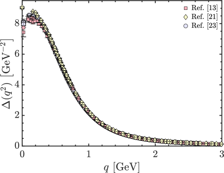
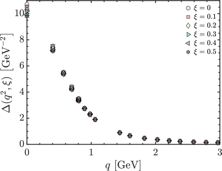
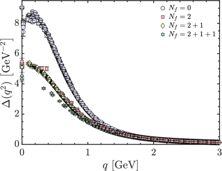
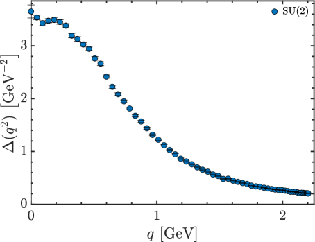
Figure 1.1: Gluon propagator, $\Delta(q^{2})$, obtained from large volume lattice simulations, all displaying a saturation at the origin. Upper left: Quenched SU(3) Landau gauge results from various lattice setups of [13, 21, 23]. Upper right: Quenched SU(3) data for various values of the gauge fixing parameter, $\xi$, from [18]. Lower left: Landau gauge SU(3) data for different numbers of dynamical quark flavors, $N_{f}$, namely: $N_{f}=0$ (blue circles) [13, 21, 23], two light degenerate quarks, $N_{f}=2$, (red squares) [16, 20], $N_{f}=2+1$ (yellow diamonds) [22], and $N_{f}=2+1+1$ (green stars) [16, 20]. Lower right: Quenched SU(2) Landau gauge data from [24]. Note that all SU(3) data are renormalized at $\mu=4.3$ GeV, whereas the SU(2) propagator is renormalized at the largest momentum available, namely $\mu=2.2$ GeV.

The physical gluon mass gap arises in the gauge sector of QCD as a result of the complicated self-interactions among gluons [31], and accounts for the exponential decay displayed by correlation functions for gauge invariant QCD observables [57]. In addition, it sets the scale for dimensionful quantities, such as glueball masses [58, 59, 60, 61, 62, 63, 64, 65, 66, 67, 68] and “chiral limit” trace anomaly [69], and cures perturbative instabilities, such as the Landau pole mentioned above. Furthermore, it leads naturally to the notion of a “maximum gluon wavelength”, above which an effective decoupling (screening) of the gluonic modes occurs [70, 71]. Moreover, the gluon mass is one of the key pillars that support the notion of the emergent hadron mass, put forth in [72, 73, 74, 75, 76, 77, 78, 79]. Last but not least, the gluon mass gap is intimately connected to the vortex picture of confinement [80, 81, 82, 83, 84, 85, 86]. The relevance of the gluon mass to confinement was further supported by the studies of the Polyakov loop [87, 88], and the related notion of the “screening” gluon mass [89].

Given the mounting evidence supporting the notion of a dynamically generated gluon mass scale, it is of the utmost importance to identify the precise field-theoretic mechanism responsible for its emergence. Given the subtle issues related to gauge invariance, an excellent point of departure is provided by Schwinger’s seminal observation regarding the connection between gauge invariance and mass [90, 91], which paved the way for the mathematically self-consistent treatment of this problem. In particular, Schwinger pointed out that, even if the gauge symmetry forbids a mass term at the level of the fundamental Lagrangian, a gauge boson may acquire a mass if its vacuum polarization function develops a pole at zero momentum transfer ($q^{2}=0$). In what follows we will refer to this fundamental idea as the “Schwinger mechanism”, and to the attendant poles at zero momentum transfer as “massless poles” or “Schwinger poles”.

The implementation of the Schwinger mechanism in the context of QCD is particularly subtle, relying on the intricate synergy between a vast array of concepts and field-theoretic techniques [92, 93, 81, 31, 46, 94, 47, 95, 96, 97, 98, 54, 55, 77, 99, 100]. In the present work we review the most salient aspects of the ongoing research in this direction, placing particular emphasis on the key developments and their main consequences. Since the mechanism itself is expressed in terms of properties occurring at the level of the gluon propagator (or, its vacuum polarization), the caveat that will be valid throughout this presentation is that the gluon mass we are exploring is the $m$ introduced above, rather than the physical gluon mass; we will be referring to this $m$ as the “gluon mass scale” throughout.

The sequence of ideas and computations that will be addressed in this work, and their organization into sections and appendices, may be summarized as follows.

Section 2: All calculations and results that we will present in this work have been carried out within the linear covariant gauges [101], with particular emphasis on the Landau gauge. Thus, starting with the classical Yang-Mills Lagrangian, a brief overview of the path integral quantization in these gauges is given, where the relevant Green functions are introduced, such as the gluon and ghost propagators, $\Delta(q^{2})$ and $D(q^{2})$, respectively, the three-gluon vertex ${\rm{I}}\!\Gamma_{\alpha\mu\nu}(q,r,p)$, and the ghost-gluon vertex, ${\rm{I}}\!\Gamma_{\alpha}(r,p,q)$. In addition, the relevant Slavnov-Taylor identities (STIs) [102, 103] are stated, and the renormalization relations that will be employed throughout are provided. All calculations are carried out using conventions and Feynman rules written in Minkowski space; the corresponding conversion to Euclidean space proceeds through the rules summarized in App. A. Moreover, the renormalization scheme adopted throughout this review is discussed in App. B.

Section 3: The physics associated with the generation of a gluon mass scale, in general, and the implementation of the Schwinger mechanism in QCD, in particular, is purely nonperturbative. In the continuum, a standard framework for dealing with nonperturbative problems are the Schwinger-Dyson equations (SDEs) [104, 105], which play the role of the equations of motion for Green (correlation) functions [106, 107, 108, 109, 110, 111, 112, 113, 71, 98, 114, 115, 116, 117]. Since this formalism will be extensively employed in this review, we outline their derivation from the generating functional, and present the diagrammatic structure of two of the most relevant cases, namely the SDEs that govern the evolution of the gluon propagator and the three-gluon vertex.

Section 4: Typically, certain basic properties, such as the transversality of the gluon self-energy, are hard to demonstrate at the diagrammatic level of the SDEs in the linear covariant gauges, especially when approximations or truncations are implemented. This problem originates primarily from the fact that the Green functions satisfy non-linear STIs (see Sec. 2); thus, the manifestation of certain fundamental features often requires extensive cancellations among several diagrams. Instead, the Green functions defined within the PT-BFM framework [46, 118], namely the fusion of the pinch technique (PT) [31, 37, 119, 120, 121, 111, 122] with the background field method (BFM) [123, 124, 125, 126, 127, 128, 129, 130, 131, 132, 133], satisfy Abelian (ghost-free) STIs. Due to this key difference, certain pivotal properties, required for the main analysis, are far more transparent and easier to demonstrate at the level of these Green functions [46, 118, 134, 135, 136]. The conversion of these results into statements at the level of the conventional Green functions (those studied on the lattice) is facilitated by a set of relations known as Background-Quantum identities (BQIs) [137, 138, 139, 111, 140], whose form simplifies considerably in the physically relevant limit of vanishing momentum transfer.

Section 5: Even though the causal assertion that gauge invariance prohibits the generation of a mass is plainly refuted by Schwinger’s observation, it is important to identify the mathematical condition that enforces the masslessness of gauge bosons when the Schwinger mechanism is not active. In perturbation theory, dimensional regularization guarantees the vanishing of such a mass (and the absence of quadratic divergences), due to the validity of relations of the type $\int_{k}d^{d}k/k^{2}$, or its higher-order generalization $\int_{k}d^{d}k\ln^{n}\!k^{2}/k^{2}$, $n=0,1,2...$ [31, 141]. Instead, at the nonperturbative level, the masslessness is enforced by a special relation, known as “seagull identity” [95, 54], which operates in scalar QED, in spinor QED, and, most importantly, in Yang-Mills theories and in the gauge sector of QCD. After reviewing the derivation of this identity, we demonstrate how it manifests itself at the level of the gluon SDE; this is of paramount importance because it is precisely this identity that has to be evaded in order for the gluon mass scale to arise in the $g_{\mu\nu}$ part of the gluon propagator. Certain technical issues are presented in App. C and App. D.

Section 6: The general formulation of the Schwinger mechanism is presented, and its implementation in QCD is elucidated. In particular, we explain that the massless poles arise as colored composite excitations of vanishing mass, produced through the fusion of elementary fields, such as gluons and ghosts [92, 93, 142, 31, 143, 96, 97, 98, 55, 144, 145, 146, 77, 99, 100].

Section 7: The vertices ${\rm{I}}\!\Gamma_{\alpha\mu\nu}(q,r,p)$ and ${\rm{I}}\!\Gamma_{\alpha}(r,p,q)$ possess special components, to be denoted by ${\cal V}_{\alpha\mu\nu}(q,r,p)$ and $V_{\alpha}(r,p,q)$, which are comprised by massless poles. The effects of these components are transmitted to the gluon polarization function through the corresponding SDE, which contains the vertices ${\rm{I}}\!\Gamma_{\alpha\mu\nu}(q,r,p)$ and ${\rm{I}}\!\Gamma_{\alpha}(r,p,q)$ as its main building blocks. As we explain in detail, basic physical requirements dictate that ${\cal V}_{\alpha\mu\nu}(q,r,p)$ and $V_{\alpha}(r,p,q)$ should be completely longitudinal [92, 93, 81, 31, 46, 94, 47, 95, 96, 97, 98, 54, 55, 144, 147, 145, 146, 77, 99, 100], namely contain poles in the form $q_{\alpha}/q^{2}$, $r_{\mu}/r^{2}$, $p_{\nu}/p^{2}$, and products thereof. The general tensorial structure of ${\cal V}_{\alpha\mu\nu}(q,r,p)$ is discussed in detail. Out of the entire pole structure of ${\cal V}_{\alpha\mu\nu}(q,r,p)$, the simple (order one) pole in $q^{2}$ is special, because its residue function, denoted by ${\mathbb{C}}(r^{2})$, eventually triggers the Schwinger mechanism. The corresponding residue function related to $V_{\alpha}(r,p,q)$, denoted by ${\mathcal{C}}(r^{2})$, is also introduced, even though its numerical contribution is known to be subleading [144, 146].

Section 8: In this section, one of the major results of this review is presented. In particular, by considering the $q_{\mu}q_{\nu}$ component of the gluon self-energy, we derive the equation that expresses the gluon mass scale as an integral involving precisely the pole residues ${\mathbb{C}}(r^{2})$ and ${\mathcal{C}}(r^{2})$ [96, 97, 98, 54, 55, 144], introduced in the previous section. The demonstration capitalizes on the advantages offered by the BFM formalism, using in addition two simple BQIs given in App. E.

Section 9: Under the action of the Schwinger mechanism, the STIs obeyed by the vertices are unchanged, but are now resolved with the nontrivial participation of the Schwinger poles, i.e., the terms ${\cal V}_{\alpha\mu\nu}(q,r,p)$ and $V_{\alpha}(r,p,q)$ introduced in Sec. 8. In the soft-gluon limit ($q\to 0$), this observation leads to a nontrivial modification of the Ward identity (WI) satisfied by the pole-free parts of the vertices [95, 98, 54, 146, 77, 99]. In this section, we illustrate this characteristic effect by means of a simple example, namely the BFM ghost-gluon vertex, which, in contradistinction to its conventional counterpart, satisfies a simple Abelian STI. The pivotal observation emerging from this analysis is that the displacement of the WI is controlled precisely by the corresponding residue function.

Section 10: We demonstrate in detail how the WI displacement introduced in the previous section leads to the evasion of the seagull cancellation at the level of the $g_{\mu\nu}$ component of the gluon propagator [96, 97, 98, 54, 55, 144]. In fact, one obtains precisely the same expression for the gluon mass scale derived in Section 8 from the $q_{\mu}q_{\nu}$ component, in absolute compliance with the exact transversality of the gluon self-energy.

Section 11: In this section we focus on the soft-gluon limit of the STI satisfied by the three-gluon vertex, thus determining the displacement of the associated form factor, denoted by $\mathit{L}_{{sg}}(r^{2})$. Quite importantly, the displacement is described in terms of the residue function ${\mathbb{C}}(r^{2})$, which, for this reason, is also denominated displacement function [146, 148]. This result constitutes a smoking-gun signal of the Schwinger mechanism, and sets the stage for the lattice-based extraction of ${\mathbb{C}}(r^{2})$, presented in the next section.

Section 12: The result of the previous section offers the valuable opportunity to probe the action of the Schwinger mechanism in a model-independent way. In particular, ${\mathbb{C}}(r^{2})$ is expressed in terms of quantities that are simulated on the lattice, with the exception of a partial derivative of the ghost-gluon kernel, which is computed in App. F. The detailed analysis reveals a clearly nonvanishing signal for ${\mathbb{C}}(r^{2})$ [148], with a substantial deviation from the null hypothesis value, corresponding to ${\mathbb{C}}(r^{2})=0$.

Section 13: The component ${\cal V}_{\alpha\mu\nu}(q,r,p)$ of the three-gluon vertex possesses a rich pole content, which is mathematically required when the gluon propagator entering in the corresponding STI is of the massive type. In particular, we show that the form factors accompanying mixed poles, i.e., of the type $q_{\alpha}r_{\mu}/q^{2}r^{2}$, are manifestly nonvanishing [149]; nonetheless, in the Landau gauge, they are completely transparent to the mass generation mechanism.

Section 14: In this section we address a central aspect of the problem, namely the dynamics of the Schwinger pole formation. As we explain therein, these poles appear as scalar composite excitations in the four-gluon scattering kernel that enters in the SDE of the three-gluon vertex. We introduce certain important quantities, most notably the form factor $I(q^{2})$ of the gluon-scalar transition amplitude, together with the effective scalar-gluon-gluon vertex, $B_{\mu\nu}(q,r,p)$. In addition, the gluon mass scale is expressed through the compact formula $m^{2}=g^{2}I^{2}$, with $I:=I(0)$.

Section 15: The soft-gluon limit ($q\to 0$) of some of the quantities introduced in the previous section is derived, and a useful diagrammatic representation is provided. Particularly important in this context is the limit of vertex $B_{\mu\nu}(q,r,p)$, which is described by the function $\mathbb{B}(r^{2})$. Quite interestingly, $\mathbb{B}(r^{2})$ coincides, up to a constant, with the displacement/residue function ${\mathbb{C}}(r^{2})$.

Section 16: We discuss the soft-gluon limit of the SDE satisfied by the pole-free part of the three-gluon vertex, involving the special form factor $\mathit{L}_{{sg}}(r^{2})$. This particular SDE represents an indispensable ingredient for the ensuing analysis, because it participates nontrivially in a crucial cancellation.

Section 17: Here we present a vital step towards the computation of the gluon mass scale, namely the renormalization of the dynamical equations that determine $I$, $B_{\mu\nu}(q,r,p)$, and $\mathit{L}_{{sg}}(r^{2})$. In particular, the equation for $I$ is renormalized multiplicatively, by the renormalization constant assigned to the three-gluon vertex.

Section 18: We set up the Bethe-Salpeter equation (BSE) that controls the evolution of $\mathbb{B}(r^{2})$ [100], discuss its nonlinear (cubic) nature, and carry out its renormalization.

Section 19: The nonlinear character of the BSE of the previous section is decisive for fixing the scale of the solutions found for $\mathbb{B}(r^{2})$, and, therefore, for determining the size of the displacement function ${\mathbb{C}}(r^{2})$ [100]. In this section, we explain how the scale-setting is implemented, and clarify why the sign ambiguity encountered is physically immaterial.

Section 20: It turns out that the multiplicative renormalization of the equation for $I$ may be carried out exactly, giving rise to a closed finite answer for the gluon mass scale [100]. This result becomes possible by virtue of a massive cancellation, which is activated once a judicious combination of the renormalized equations governing $\mathbb{B}(r^{2})$, $I$, and $\mathit{L}_{{sg}}(r^{2})$, has been exploited.

Section 21: The cancellation exposed in Sec. 20 occurs for a very specific mathematical reason, namely the Fredholm alternatives theorem [150, 151]. In this section we state this theorem, and illustrate its function at the level of the dynamical equations that we employ. The upshot of these considerations is that the gluon mass scale is proportional to the nonlinear term in the BSE for $\mathbb{B}(r^{2})$, precisely because its inclusion allows the evasion of Fredholm’s theorem [100].

Section 22: In this section we carry out a detailed numerical analysis of the final equations, with all previous observations taking into account. A central input for this treatment is the four-gluon kernel, which is appropriately modeled, using its one-loop exchange approximation as our point of departure. The results found for $m^{2}$ are contrasted with the saturation point of the gluon propagator found in lattice simulations, while ${\mathbb{C}}(r^{2})$ is compared with the curve obtained from the construction described in Sec. 12.

Section 23: In this final section we present our conclusions, and a discussion of the open problems and possible future directions.

We finally point out that alternative approaches to the gluon mass have been put forth over the years; a representative sample of the extensive literature on this subject is given by [43, 152, 153, 154, 155, 156, 157, 48, 158, 159, 160, 161, 50, 162, 163, 164, 51, 165, 53, 166, 167, 168, 169, 57], and references therein.

2 General framework: covariantly quantized Yang-Mills theories

The classical Lagrangian density, ${\cal L}_{\mathrm{cl}}$, of a pure Yang-Mills theory based on an SU($N$) gauge group is given by

$${\cal L}_{\mathrm{cl}}=-\frac{1}{4}F^{a}_{\mu\nu}F^{a\mu\nu}\,,$$ (2.1)

where

$$F^{a}_{\mu\nu}=\partial_{\mu}A^{a}_{\nu}-\partial_{\nu}A^{a}_{\mu}+gf^{abc}A^{b}_{\mu}A^{c}_{\nu}\,$$ (2.2)

is the antisymmetric field tensor, $A^{a}_{\mu}(x)$ denotes the gauge field, with $a=1,\dots,N^{2}-1$, $f^{abc}$ stands for the totally antisymmetric structure constants of the SU($N$) gauge group, and $g$ is the gauge coupling. The theory defined by Eqs. (2.1) and (2.2) is invariant under the infinitesimal local gauge transformations

$$A^{a}_{\mu}\to A^{a}_{\mu}+g^{-1}\partial_{\mu}\theta^{a}+f^{abc}A^{b}_{\mu}\theta^{c}\,,$$ (2.3)

where $\theta^{a}(x)$ are the angles describing rotations in the space of SU($N$) matrices.

When the theory is quantized following the standard Faddeev-Popov procedure [5], the resulting Lagrangian density ${\cal L}_{\mathrm{YM}}$ consists of ${\cal L}_{\mathrm{cl}}$, the contribution from the ghosts, ${\cal L}_{\mathrm{gh}}$, and the covariant gauge-fixing term, ${\cal L}_{\mathrm{gf}}$, namely

$${\cal L}_{\mathrm{YM}}={\cal L}_{\mathrm{cl}}+{\cal L}_{\mathrm{gh}}+{\cal L}_{\mathrm{gf}}\,,$$ (2.4)

where

$${\cal L}_{\mathrm{gh}}=-{\overline{c}}^{a}\partial^{\mu}D_{\mu}^{ab}c^{b}\,,\qquad\qquad{\cal L}_{\mathrm{gf}}=\frac{1}{2\xi}(\partial^{\mu}A^{a}_{\mu})^{2}\,.$$ (2.5)

In Eq. (2.5), $c^{a}(x)$ and ${\overline{c}}^{a}(x)$ are the ghost and anti-ghost fields, respectively, while

$$D_{\mu}^{ab}=\partial_{\mu}\delta^{ab}+gf^{amb}A^{m}_{\mu}\,,$$ (2.6)

is the covariant derivative in the adjoint representation. Finally, $\xi$ denotes the gauge-fixing parameter, where the choice $\xi=0$ defines the Landau gauge, while $\xi=1$ corresponds to the Feynman–’t Hooft gauge.

The Lagrangian defined in Eqs. (2.4) and (2.5) gives rise to the standard set of Feynman rules, see, e.g., the Appendix B of [111], used in the majority of physical applications. We emphasize that throughout this work we will be working in the Minkowski space, where all intermediate results will be derived, employing the aforementioned Feynman rules. The numerical treatment of the equations requires the final transition from the Minkowski to the Euclidean space, which will be carried out following standard transformation rules and conventions, given in App. A. Note also that, when reporting formulas, we will keep the gauge group general, specializing to the case $N=3$ only in the numerical evaluation of the final results.

The transition from the pure Yang-Mills theory (with $N=3$) to real-world QCD requires the addition to ${\cal L}_{\mathrm{YM}}$ of the corresponding kinetic and interaction terms for the quark fields. In this review we will focus exclusively on the pure Yang-Mills case, which captures faithfully the bulk of the dynamics responsible for the emergence of a gluon mass [170]; consequently, the aforementioned quark terms will be omitted entirely from the Lagrangian.

The central elements of our analysis are the $n$-point Green functions, or, equivalently, correlation functions, defined as vacuum expectation values of time-ordered products of $n$ fields. For instance, in configuration space, we have for the gluon two-point function, also known as gluon propagator,

$$\Delta^{ab}_{\mu\nu}(x,y)=\langle 0|T\left(A^{a}_{\mu}(x)\,A^{b}_{\nu}(y)\right)|0\rangle\,,$$ (2.7)

where $T$ denotes the standard time-ordering operation. The transition to the momentum space, implemented by the standard Fourier transform (FT), expresses the Green functions in terms of their incoming momenta; thus, in the case of the gluon propagator, one has that $\Delta^{ab}_{\mu\nu}(x,y)\overset{{\rm FT}}{\rightarrow}\Delta^{ab}_{\mu\nu}(q)$. Completely analogous definitions apply for all higher Green functions, which will be generally denoted by the letter ${\rm{I}}\!\Gamma$, carrying appropriate color, Lorentz, and momentum indices.

The Green functions are formally obtained through functional differentiation of the generating functional, $Z[J,\eta,\bar{\eta}]$, defined as [171, 172, 173]

$$Z[J,\eta,\bar{\eta}]=\int\mathcal{D}A\,\mathcal{D}c\,\mathcal{D}\bar{c}\,\exp\left\{iS_{\mathrm{YM}}[A,c,\bar{c}]+i\int d^{4}x\left[J^{a}_{\mu}A^{a\mu}+{\bar{\eta}}^{a}c^{a}+{\bar{c}}^{a}\eta^{a}\right]\right\}\,,$$ (2.8)

where

$$S_{\mathrm{YM}}[A,c,\bar{c}]=\int\!d^{4}x\,{\cal L}_{\mathrm{YM}}\,,$$ (2.9)

is the action, $J(x)$, $\eta(x)$, and $\bar{\eta}(x)$ are appropriate sources, and the path-integral measure is defined as $\mathcal{D}A:=\prod_{x}\prod_{\alpha,\mu}dA^{a}_{\mu}$, with completely analogous definitions for $\mathcal{D}c$ and $\mathcal{D}\bar{c}$ . Specifically, a Green function composed by $n$ fields is given by

$$\langle 0|T\left(\phi_{i_{1}}(x_{1})\ldots\phi_{i_{n}}(x_{n})\right)|0\rangle=\frac{\int\mathcal{D}A\,\mathcal{D}c\,\mathcal{D}\bar{c}\,\phi_{i_{1}}(x_{1})\ldots\phi_{i_{n}}(x_{n})e^{iS_{\mathrm{YM}}[A,c,\bar{c}]}}{\int\mathcal{D}A\,\mathcal{D}c\,\mathcal{D}\bar{c}\,e^{iS_{\mathrm{YM}}[A,c,\bar{c}]}}=\left.\frac{(-i)^{n}}{Z[0,0,0]}\frac{\delta^{n}Z}{\delta j_{i_{1}}(x_{i})\ldots\delta j_{i_{n}}(x_{n})}\right|_{j_{k}=0}\,,$$ (2.10)

where, to take into account the Grassmann nature of the (anti)ghost fields and their sources, the functions $\phi_{i}$ and $j_{i}$ denote

$$\phi_{i}=\{A,c,\bar{c}\}\,,\qquad j_{i}=\{J,\bar{\eta},-\eta\}\,.$$ (2.11)

The generating functional $Z[J,\eta,\bar{\eta}]$ contains all possible Feynman diagrams, including disconnected contributions. In practice, it suffices to compute the one-particle irreducible (1PI) Green functions, because all other diagrams can be obtained as combinations of them. It is therefore advantageous to generalize the $Z[J,\eta,\bar{\eta}]$, such that only 1PI Green functions will be generated through appropriate functional differentiation.

To that end, one first defines the generating functional of connected diagrams, $W[J,\eta,\bar{\eta}]:=-i\ln Z[J,\eta,\bar{\eta}]$. Then, the 1PI Green functions are obtained from the effective action, $\Gamma[A,c,\bar{c}]$, defined as the Legendre transform of $W[J,\eta,\bar{\eta}]$, i.e.,

$$\Gamma[A_{\rm{\scriptscriptstyle cl}},c_{\rm{\scriptscriptstyle cl}},\bar{c}_{\rm{\scriptscriptstyle cl}}]=W[J,\eta,\bar{\eta}]-\int d^{4}x\left[J^{a}_{\mu}(x)A_{\rm{\scriptscriptstyle cl}}^{a\mu}(x)+{\bar{\eta}}^{a}(x)c_{\rm{\scriptscriptstyle cl}}^{a}(x)+{\bar{c}}_{\rm{\scriptscriptstyle cl}}^{a}(x)\eta^{a}(x)\right]\,,$$ (2.12)

where $\phi_{\rm{\scriptscriptstyle cl}}$ denotes the “classical” counterpart of a field $\phi$, i.e., its vacuum expectation value. Indeed, it follows from Eqs. (2.10) and (2.12) that

$$A_{{\rm{\scriptscriptstyle cl}}}^{a\mu}(x):=\langle 0|A^{a\mu}(x)|0\rangle=\frac{\delta W}{\delta J^{a}_{\mu}(x)}\,,\qquad c_{\rm{\scriptscriptstyle cl}}^{a}(x):=\langle 0|c^{a}(x)|0\rangle=\frac{\delta W}{\delta{\bar{\eta}}^{a}(x)}\,,\qquad{\bar{c}}_{\rm{\scriptscriptstyle cl}}^{a}(x):=\langle 0|{\bar{c}}^{a}(x)|0\rangle=-\frac{\delta W}{\delta\eta^{a}(x)}\,.$$ (2.13)

Moreover, the sources are related to $\Gamma[J,\eta,\bar{\eta}]$ and the $\phi_{\rm{\scriptscriptstyle cl}}$ by

$$J^{a}_{\mu}(x)=-\frac{\delta\Gamma}{\delta A^{a\mu}_{\rm{\scriptscriptstyle cl}}(x)}\,,\qquad\qquad\eta^{a}(x)=-\frac{\delta\Gamma}{\delta{\bar{c}}^{a}_{\rm{\scriptscriptstyle cl}}(x)}\,,\qquad\qquad{\bar{\eta}}^{a}(x)=\frac{\delta\Gamma}{\delta c^{a}_{\rm{\scriptscriptstyle cl}}(x)}\,.$$ (2.14)

The $n$-point 1PI Green functions for $n\geq 3$ are obtained from $\Gamma[J,\eta,\bar{\eta}]$ by taking functional derivatives and setting all classical fields to zero. Specifically [171, 172, 173],

$$\langle 0|T\left(\phi_{1}(x_{1})\phi_{2}(x_{2})\ldots\phi_{n}(x_{n})\right)|0\rangle_{\text{1PI}}=\left.\frac{\delta^{n}\Gamma}{\delta\phi_{{\rm{\scriptscriptstyle cl}},1}(x_{1})\delta\phi_{{\rm{\scriptscriptstyle cl}},2}(x_{2})\ldots\phi_{{\rm{\scriptscriptstyle cl}},n}(x_{n})}\right|_{\phi_{{\rm{\scriptscriptstyle cl}},k}=0}\,.$$ (2.15)

Exceptionally, the two-point Green functions are related to inverses of derivatives. This follows from the combination of Eq. (2.14) with the trivial identity,

$$\frac{\delta\phi_{{\rm{\scriptscriptstyle cl}},i}(x)}{\delta\phi_{{\rm{\scriptscriptstyle cl}},j}(y)}=\delta^{ij}\delta(x-y)=\int\!d^{4}z\,\frac{\delta j_{k}(z)}{\delta\phi_{{\rm{\scriptscriptstyle cl}},j}(y)}\frac{\delta\phi_{{\rm{\scriptscriptstyle cl}},i}(x)}{\delta j_{k}(z)}=-\int\!d^{4}z\,\frac{\delta^{2}\Gamma}{\delta\phi_{{\rm{\scriptscriptstyle cl}},j}(y)\delta\phi_{{\rm{\scriptscriptstyle cl}},k}(z)}\frac{\delta^{2}W}{\delta j_{k}(z)\delta j_{i}(x)}\,,$$ (2.16)

which together imply

$$\frac{\delta^{2}W}{\delta j_{i}(x)\delta j_{j}(y)}=-\left(\frac{\delta^{2}\Gamma}{\delta\phi_{{\rm{\scriptscriptstyle cl}},i}(x)\delta\phi_{{\rm{\scriptscriptstyle cl}},j}(y)}\right)^{-1}\,.$$ (2.17)

Hence, setting the sources to zero and using Eq. (2.10), one finds that the propagators are related to the effective action through

$$\langle 0|T\left(\phi_{1}(x)\phi_{2}(y)\right)|0\rangle_{\text{1PI}}=\left.-i\frac{\delta^{2}W}{\delta j_{1}(x)\delta j_{2}(y)}\right|_{j_{k}=0}=\left.i\left(\frac{\delta^{2}\Gamma}{\delta\phi_{{\rm{\scriptscriptstyle cl}},1}(x)\delta\phi_{{\rm{\scriptscriptstyle cl}},2}(y)}\right)^{-1}\right|_{\phi_{{\rm{\scriptscriptstyle cl}},k}=0}\,.$$ (2.18)

In the present work we will mainly deal with the following Green functions:

1. The gluon propagator $\Delta^{ab}_{\mu\nu}(q,\xi)=-i\delta^{ab}\Delta_{\mu\nu}(q,\xi)$, which for a general value of $\xi$ has the form

   $$\Delta_{\mu\nu}(q,\xi)=P_{\mu\nu}(q)\Delta(q^{2},\xi)+\xi\,q_{\mu}q_{\nu}/{q^{4}}\,,\qquad\qquad{P}_{\mu\nu}(q):=g_{\mu\nu}-q_{\mu}q_{\nu}/{q^{2}}\,;$$ (2.19)

   at tree-level, $\Delta_{0}(q^{2},\xi)=1/q^{2}$. The scalar function $\Delta(q^{2},\xi)$ is related to the gluon self-energy, $\Pi_{\mu\nu}(q,\xi)$,

   $$\Pi_{\mu\nu}(q,\xi)=\Pi(q^{2},\xi)P_{\mu\nu}(q)$$ (2.20)

   through

   $$\Delta^{-1}(q^{2},\xi)=q^{2}+i\Pi(q^{2},\xi)\,.$$ (2.21)

   In the Landau gauge ($\xi=0$), the gluon propagator becomes completely transverse, namely

   $$\Delta_{\mu\nu}(q)=P_{\mu\nu}(q)\Delta(q^{2})\,,\qquad\qquad\Delta^{-1}(q^{2})=q^{2}+i\Pi(q^{2})\,,$$ (2.22)

   In addition, it is convenient to introduce the dimensionless gluon dressing function, denoted by ${\cal Z}(q^{2})$, and defined as

   $${\cal Z}(q^{2})=q^{2}\Delta(q^{2})\,.$$ (2.23)

2. The ghost propagator $D^{ab}(q)=i\delta^{ab}D(q^{2})$, and its dressing function, $F(q^{2})$, defined as

   $$F(q^{2})=q^{2}D(q^{2})\,;$$ (2.24)

   at tree level, $F_{0}(q^{2})=1$.

3. The three-gluon vertex, ${\cal G}^{abc}_{\alpha\mu\nu}(q,r,p)$, which is cast in the form

   $${\cal G}^{abc}_{\alpha\mu\nu}(q,r,p)=g\,{\rm{I}}\!\Gamma^{abc}_{\alpha\mu\nu}(q,r,p)\,,\qquad\qquad{\rm{I}}\!\Gamma^{abc}_{\alpha\mu\nu}(q,r,p)=f^{abc}{\rm{I}}\!\Gamma_{\alpha\mu\nu}(q,r,p)\,,$$ (2.25)

   as shown in Fig. 2.1; at tree level,

   $$\Gamma_{\!0\,\alpha\mu\nu}(q,r,p)=(q-r)_{\nu}g_{\alpha\mu}+(r-p)_{\alpha}g_{\mu\nu}+(p-q)_{\mu}g_{\nu\alpha}\,.$$ (2.26)

   The transition from ${\cal G}\to{\rm{I}}\!\Gamma$ will be employed later on [see Secs. 14 and 16], in the context of the SDE governing the three-gluon vertex, where a factor $g$ will be canceled from both sides of the equation.

4. The ghost-gluon vertex, ${\rm{I}}\!\Gamma^{abc}_{\alpha}(r,p,q)=-gf^{abc}{\rm{I}}\!\Gamma_{\alpha}(r,p,q)$; at tree level,

   $$\Gamma_{\!0\,\alpha}(r,p,q)=r_{\alpha}\,.$$ (2.27)

5. The 1PI four-gluon vertex, which must be extracted from the amputated part of the four-point function $\mathcal{C}^{abcd}_{\mu\nu\rho\sigma}(q,r,p,t)$, as [174]

   $$\mathcal{C}^{abcd}_{\mu\nu\rho\sigma}(q,r,p,t)=-ig^{2}{\rm{I}}\!\Gamma^{abcd}_{\mu\nu\rho\sigma}(q,r,p,t)\,+\,\dots,$$ (2.28)

   where the ellipsis denotes one-particle reducible contributions, built out of the gluon propagators and three-gluon vertices. At tree level,

   $$\Gamma^{abcd}_{\!0\,\mu\nu\rho\sigma}=f^{adx}f^{cbx}\left(g_{\mu\rho}g_{\nu\sigma}-g_{\mu\nu}g_{\rho\sigma}\right)+f^{abx}f^{dcx}\left(g_{\mu\sigma}g_{\nu\rho}-g_{\mu\rho}g_{\nu\sigma}\right)+f^{acx}f^{dbx}\left(g_{\mu\sigma}g_{\nu\rho}-g_{\mu\nu}g_{\rho\sigma}\right)\,.$$ (2.29)

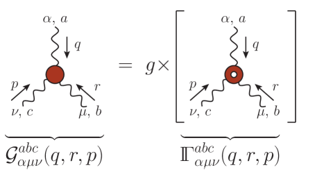
Figure 2.1: Diagrammatic conventions for the fully dressed three-gluon vertex (left) and its tree-level counterpart (right).

Note that, due to the inclusion of the terms ${\cal L}_{\mathrm{gh}}$ and ${\cal L}_{\mathrm{gf}}$ given in Eq. (2.5), the final ${\cal L}_{\mathrm{YM}}$ in Eq. (2.4) is no longer invariant under the local gauge transformations of Eq. (2.3); instead, it is invariant under the global BRST transformations [6, 7, 8]. Specifically, setting

$$c^{a}=(\rho^{a}+i\sigma^{a})/\sqrt{2}\,,\qquad\qquad{\bar{c}}^{a}=(\rho^{a}-i\sigma^{a})/\sqrt{2}\,,$$ (2.30)

where $\rho^{a}$ and $\sigma^{a}$ are real Grassmann fields, we have that ${\cal L}_{\mathrm{YM}}$ is invariant under the combined transformations

$$\delta A^{a}_{\mu}=\omega D_{\mu}\sigma^{a}\,,\qquad\delta\rho^{a}=-i\omega\partial^{\mu}A^{a}_{\mu}/\xi\,,\qquad\delta\sigma^{a}=-g\omega f^{abc}\sigma^{b}\sigma^{c}/2\,,$$ (2.31)

where $\omega$ is a Grassmann variable ($\omega^{2}=0$) that does not depend on the space-time coordinate $x$.

A major consequence of the BRST symmetry are the STIs [102, 103], which replace the Ward-Takahashi identities (WTIs) known from QED [175, 176], and in general, from Abelian theories. The main difference between STIs and WTIs is that, while the WTIs are simple all-order generalizations of tree-level identities, the STIs receive non-trivial contributions from the ghost sector of the theory, which deform their tree-level expressions.

In the case of the gluon propagator, the corresponding STI affirms the transversality of the self-energy $\Pi_{\mu\nu}(q)$, namely

$$q^{\mu}\Pi_{\mu\nu}(q)=q^{\nu}\Pi_{\mu\nu}(q)=0\,,$$ (2.32)

a property valid for any value of the gauge-fixing parameter $\xi$.

Throughout this review we will make extensive use of the STI satisfied by the three-gluon vertex, ${\rm{I}}\!\Gamma_{\alpha\mu\nu}(q,r,p)$, given by

$$q^{\alpha}{\rm{I}}\!\Gamma_{\alpha\mu\nu}(q,r,p)=F(q^{2})\left[\Delta^{-1}(p^{2})P_{\nu}^{\sigma}(p)H_{\sigma\mu}(p,q,r)-\Delta^{-1}(r^{2})P_{\mu}^{\sigma}(r)H_{\sigma\nu}(r,q,p)\right]\,,$$ (2.33)

where $H_{\nu\mu}(r,p,q)$ denotes the so-called ghost-gluon kernel [2, 177, 178, 179, 180, 181], a composite operator that is diagrammatically depicted in Fig. 2.2. When contracted with either $r^{\mu}$ or $p^{\nu}$, ${\rm{I}}\!\Gamma_{\alpha\mu\nu}(q,r,p)$ satisfies completely analogous STIs, obtained from Eq. (2.33) by applying cyclic permutations of the indices and momenta assigned to the external legs.

Figure 2.2: Diagrammatic representation of the ghost-gluon scattering kernel, $H_{\nu\mu}(r,p,q)$. White circles indicate fully-dressed propagators, and the grey ellipse represents the ${\bar{c}}cA_{\mu}A_{\nu}$ amplitude. At tree level, $H_{\nu\mu}^{0}=g_{\nu\mu}$.

The corresponding STI satisfied by ghost-gluon vertex, ${\rm{I}}\!\Gamma_{\alpha}(r,p,q)$, reads [107]

$$F^{-1}(q^{2})\,q^{\alpha}{\rm{I}}\!\Gamma_{\alpha}(r,p,q)+F^{-1}(p^{2})\,p^{\alpha}{\rm{I}}\!\Gamma_{\alpha}(r,q,p)=-r^{2}F^{-1}(r^{2})U(r,q,p)\,,$$ (2.34)

where $U(r,q,p)$ is an interaction kernel containing only ghost fields; its tree-level value is $U^{0}(r,q,p)=1$. Note that the contraction of ${\rm{I}}\!\Gamma_{\alpha}(r,p,q)$ by $q^{\alpha}$ is expressed in terms of the corresponding contraction by $p^{\alpha}$, a fact that reduces considerably the usefulness of the STI in Eq. (2.34); we report it mainly for the purpose of contrasting it with its simpler BFM counterpart, given in Eq. (4.4).

The STI for the conventional four-gluon vertex is far more involved; it may be found in Eq. (C.24) of [111].

We end this section by introducing the formal elements entering in the procedure of multiplicative renormalization, which is applied to all nonperturbative results presented in this work. Denoting by the index “R” the renormalized quantities, we have

$$\Delta_{{\scriptscriptstyle R}}(q^{2}) =Z^{-1}_{A}\Delta(q^{2})\,, \quad\quad\quad{\rm{I}}\!\Gamma^{\mu}_{\!\!{\scriptscriptstyle R}}(q,p,r) =Z_{1}{\rm{I}}\!\Gamma^{\mu}(q,p,r)\,,$$

$$D_{\!{\scriptscriptstyle R}}(q^{2}) =Z^{-1}_{c}D(q^{2})\,, \quad\quad\quad{\rm{I}}\!\Gamma^{\alpha\mu\nu}_{\!\!{\scriptscriptstyle R}}(q,r,p) =Z_{3}{\rm{I}}\!\Gamma^{\alpha\mu\nu}(q,r,p)\,,$$

$$g_{{\scriptscriptstyle R}} =Z_{g}^{-1}g\,, \quad\quad\quad{\rm{I}}\!\Gamma^{abcd}_{\!\!{\scriptscriptstyle R}\,\alpha\beta\mu\nu}(q,r,p,t) =Z_{4}{\rm{I}}\!\Gamma^{abcd}_{\alpha\beta\mu\nu}(q,r,p,t)\,,$$ (2.35)

where $Z_{A}$ and $Z_{c}$ are the wave function renormalization constants of the gluon and ghost fields, $Z_{3}$, $Z_{1}$, and $Z_{4}$ are the renormalization constants of the three-gluon, ghost-gluon, and four-gluon vertices, and $Z_{g}$ is the coupling renormalization constant. Note that, by virtue of Taylor’s theorem [102], $Z_{1}$ is finite in the Landau gauge; its precise value depends on the renormalization scheme adopted [182, 148, 99]. In this work, we employ a variation of the momentum subtraction scheme (MOM) [183, 184, 185], namely the asymmetric MOM scheme [186, 187, 188, 189, 182, 190, 23], discussed in App. B.

In addition, we employ the exact relations

$$Z_{g}^{-1}=Z_{1}^{-1}Z_{A}^{1/2}Z_{c}\,=Z_{3}^{-1}Z_{A}^{3/2}\,=Z_{4}^{-1/2}Z_{A}\,,$$ (2.36)

which are a direct consequence of the fundamental STIs [191, 172].

3 Schwinger-Dyson equations

The main nonperturbative tool employed throughout this review is the set of integral equations known as SDEs, which play the role of the equations of motion for the Green functions of the theory. The SDEs are obtained formally from the generating functional $Z[J,\eta,\bar{\eta}]$, following a procedure that we outline below; for further details, see [171, 173, 106, 192, 193]. For an an alternative continuum framework, denominated “functional renormalization group”, see e.g.,  [194, 195, 155, 196, 197, 198, 199, 117, 200, 201].

The starting point of the derivation of the SDEs is the observation that under appropriate boundary conditions the functional integral of a total functional derivative vanishes. In particular,

$$0= \,\int\mathcal{D}A\,\mathcal{D}c\,\mathcal{D}\bar{c}\,\frac{\delta}{\delta c^{a}(x)}\exp\left\{iS_{\mathrm{YM}}+i\int d^{4}w\left[J^{a}_{\mu}(w)A^{a\mu}(w)+{\bar{\eta}}^{a}(w)c^{a}(w)+{\bar{c}}^{a}(w)\eta^{a}(w)\right]\right\}$$

$$= \,i\int\mathcal{D}A\,\mathcal{D}c\,\mathcal{D}\bar{c}\,\left[\frac{\delta S_{\mathrm{YM}}}{\delta c^{a}(x)}-\bar{\eta}^{a}(x)\right]\exp\left\{iS_{\mathrm{YM}}+i\int d^{4}w\left[J^{a}_{\mu}(w)A^{a\mu}(w)+{\bar{\eta}}^{a}(w)c^{a}(w)+{\bar{c}}^{a}(w)\eta^{a}(w)\right]\right\}\,.$$ (3.1)

The last line leads directly to the master SDE

$$\left\{\frac{\delta S_{\mathrm{YM}}}{\delta c^{a}(x)}\left[\frac{\delta}{i\delta j}\right]-\bar{\eta}^{a}(x)\right\}Z[J,\eta,\bar{\eta}]=0\,,$$ (3.2)

where the argument $[\delta/i\delta j]$ denotes the substitution $\phi_{i}\to\delta/i\delta j_{i}$ for every field in the expression for $\delta S_{\mathrm{YM}}/\delta c^{a}(x)$. Through similar steps, one obtains two additional master SDEs, namely

$$\left\{\frac{\delta S_{\mathrm{YM}}}{\delta\bar{c}^{a}(x)}\left[\frac{\delta}{i\delta j}\right]+\eta^{a}(x)\right\}Z[J,\eta,\bar{\eta}]= \,0\,,$$ (3.3)

$$\left\{\frac{\delta S_{\mathrm{YM}}}{\delta A^{a\mu}(x)}\left[\frac{\delta}{i\delta j}\right]+J_{\mu}^{a}(x)\right\}Z[J,\eta,\bar{\eta}]= \,0\,.$$ (3.4)

Then, differentiating Eqs. (3.2), (3.3) and (3.4) with respect to further sources, and setting the sources to zero in the end, one obtains the SDEs for the Green functions.

In order to derive a master SDE for the 1PI Green functions, we start by substituting $Z=e^{iW}$ in Eq. (3.2), and use the identity

$$e^{-iW}f\left(\frac{\delta}{i\delta j}\right)e^{iW}=f\left(\frac{\delta W}{\delta j}+\frac{i\delta}{\delta j}\right)\,,$$ (3.5)

to obtain

$$\frac{\delta S_{\mathrm{YM}}}{\delta c^{a}(x)}\left[\frac{\delta W}{\delta j}+\frac{\delta}{i\delta j}\right]=\bar{\eta}^{a}(x)\,.$$ (3.6)

Then, combining Eqs. (2.14) and (2.17) with the chain rule,

$$\frac{\delta}{i\delta j_{i}(x)}=-i\int\!d^{4}z\frac{\delta\phi_{{\rm{\scriptscriptstyle cl}},i}(z)}{\delta j(x)}\frac{\delta}{\delta\phi_{{\rm{\scriptscriptstyle cl}},i}(z)}=-i\int\!d^{4}z\frac{\delta^{2}W}{\delta j(x)\delta j_{i}(z)}\frac{\delta}{\delta\phi_{{\rm{\scriptscriptstyle cl}},i}(z)}=i\int\!d^{4}z\left(\frac{\delta^{2}\Gamma}{\delta\phi_{{\rm{\scriptscriptstyle cl}},i}(x)\delta\phi_{{\rm{\scriptscriptstyle cl}},j}(z)}\right)^{-1}\frac{\delta}{\delta\phi_{{\rm{\scriptscriptstyle cl}},j}(z)}\,,$$ (3.7)

yields the final equation,

$$\frac{\delta S_{\mathrm{YM}}}{\delta c^{a}(x)}\left[\phi_{\rm{\scriptscriptstyle cl}}+i\int\!d^{4}z\left(\frac{\delta^{2}\Gamma}{\delta\phi_{{\rm{\scriptscriptstyle cl}}}\delta\phi_{{\rm{\scriptscriptstyle cl}},j}(z)}\right)^{-1}\frac{\delta}{\delta\phi_{{\rm{\scriptscriptstyle cl}},j}(z)}\right]=\frac{\delta\Gamma}{\delta c_{\rm{\scriptscriptstyle cl}}^{a}(x)}\,.$$ (3.8)

Applying similar steps to Eqs. (3.3) and (3.4), one obtains

$$\frac{\delta S_{\mathrm{YM}}}{\delta\bar{c}^{a}(x)}\left[\phi_{\rm{\scriptscriptstyle cl}}+i\int\!d^{4}z\left(\frac{\delta^{2}\Gamma}{\delta\phi_{{\rm{\scriptscriptstyle cl}}}\delta\phi_{{\rm{\scriptscriptstyle cl}},j}(z)}\right)^{-1}\frac{\delta}{\delta\phi_{{\rm{\scriptscriptstyle cl}},j}(z)}\right]= \,\frac{\delta\Gamma}{\delta{\bar{c}}_{\rm{\scriptscriptstyle cl}}^{a}(x)}\,,$$ (3.9)

$$\frac{\delta S_{\mathrm{YM}}}{\delta A^{a\mu}(x)}\left[\phi_{\rm{\scriptscriptstyle cl}}+i\int\!d^{4}z\left(\frac{\delta^{2}\Gamma}{\delta\phi_{{\rm{\scriptscriptstyle cl}}}\delta\phi_{{\rm{\scriptscriptstyle cl}},j}(z)}\right)^{-1}\frac{\delta}{\delta\phi_{{\rm{\scriptscriptstyle cl}},j}(z)}\right]= \,\frac{\delta\Gamma}{\delta A_{\rm{\scriptscriptstyle cl}}^{a\mu}(x)}\,.$$ (3.10)

Finally, the SDEs for specific 1PI Green functions are obtained by taking derivatives of Eqs. (3.8), (3.9) and (3.10), and setting the classical fields to zero.

As a concrete example, we consider the simplest SDE in Yang-Mills theory, namely the equation governing the ghost propagator. Since we seek an equation for $\delta^{2}\Gamma/\delta\bar{c}^{b}(y)\delta c^{a}(x)$, it is convenient to start from Eq. (3.8). Then, only the term ${\cal L}_{\mathrm{gh}}$ of the Lagrangian contributes. Specifically,

$$\frac{\delta S_{\mathrm{YM}}}{\delta c^{a}(x)}=-\partial^{2}{\bar{c}}^{a}(x)-gf^{mna}A^{m\mu}(x)\partial_{\mu}{\bar{c}}^{n}(x)\,,$$ (3.11)

and the master equation of Eq. (3.8) reads explicitly,

$$\frac{\delta\Gamma}{\delta c_{\rm{\scriptscriptstyle cl}}^{a}(x)}=-\partial^{2}{\bar{c}}^{a}(x)-gf^{mna}\left[A_{\rm{\scriptscriptstyle cl}}^{m\mu}(x)\partial^{\mu}{\bar{c}}_{\rm{\scriptscriptstyle cl}}^{n}(x)-i\partial^{\mu}\left(\frac{\delta^{2}\Gamma}{\delta A_{{\rm{\scriptscriptstyle cl}}}^{m\mu}(x)\delta{\bar{c}}_{\rm{\scriptscriptstyle cl}}^{n}(x)}\right)^{-1}\right]\,.$$ (3.12)

Then, differentiating with respect to ${\bar{c}}_{\rm{\scriptscriptstyle cl}}^{b}(y)$ and setting the classical fields to zero, we obtain

$$\frac{\delta^{2}\Gamma}{\delta{\bar{c}}_{\rm{\scriptscriptstyle cl}}^{b}(y)\delta c_{\rm{\scriptscriptstyle cl}}^{a}(x)}=-\delta^{ab}\partial^{2}\delta(x-y)-igf^{mna}\partial^{\mu}\left.\frac{\delta}{{\bar{c}}_{\rm{\scriptscriptstyle cl}}^{b}(y)}\left(\frac{\delta^{2}\Gamma}{\delta A_{{\rm{\scriptscriptstyle cl}}}^{m\mu}(x)\delta{\bar{c}}_{\rm{\scriptscriptstyle cl}}^{n}(x)}\right)^{-1}\right|_{\phi_{\rm{\scriptscriptstyle cl}}=0}\,.$$ (3.13)

At this point, the derivative of an inverse in the last term of Eq. (3.13) can be rewritten as

$$\frac{\delta}{\delta\phi_{{\rm{\scriptscriptstyle cl}},i}(x)}\left(\frac{\delta\Gamma}{\delta\phi_{{\rm{\scriptscriptstyle cl}},j}(y)\delta\phi_{{\rm{\scriptscriptstyle cl}},k}(z)}\right)^{-1}\!\!=-\int\!d^{4}u\,d^{4}v\left(\frac{\delta\Gamma}{\delta\phi_{{\rm{\scriptscriptstyle cl}},j}(y)\delta\phi_{{\rm{\scriptscriptstyle cl}},m}(u)}\right)^{-1}\!\!\frac{\delta^{3}\Gamma}{\delta\phi_{{\rm{\scriptscriptstyle cl}},m}(u)\delta\phi_{{\rm{\scriptscriptstyle cl}},i}(x)\phi_{{\rm{\scriptscriptstyle cl}},n}(v)}\left(\frac{\delta\Gamma}{\delta\phi_{{\rm{\scriptscriptstyle cl}},n}(v)\delta\phi_{{\rm{\scriptscriptstyle cl}},k}(z)}\right)^{-1}\!\!\,.$$ (3.14)

So, after identifying the propagators and vertices through Eqs. (2.15) and (2.18), we cast Eq. (3.13) in the form

$$[D^{ab}(x-y)]^{-1}= \,i\delta^{ab}\partial^{2}\delta(x-y)-gf^{mna}\partial_{\mu}\int\!d^{4}u\,d^{4}v\,\Delta_{mc}^{\mu\nu}(x-u){\rm{I}}\!\Gamma_{\nu}^{cbd}(y,v,u)D^{dn}(v-x)\,.$$ (3.15)

Noting that $i\delta^{ab}\partial^{2}\delta(x-y)$ and $gf^{mna}\partial_{\mu}$ are the tree-level inverse ghost propagator and ghost-gluon vertex, respectively, we arrive at the ghost SDE in configuration space.

Finally, a Fourier transform of Eq. (3.15) leads to the momentum space SDE for the ghost propagator; suppressing color, we get the equation

$$D^{-1}(q^{2})= \,D^{-1}_{0}(q^{2})-\int_{k}\Gamma^{\!0\,\mu}(k,q,-k-q)\Delta^{\mu\nu}(k+q)D(k^{2}){\rm{I}}\!\Gamma_{\nu}(-q,-k,k+q)\,,$$ (3.16)

represented diagrammatically in Fig. 3.1. Note that, throughout this work, we denote by

$$\int_{k}:=\frac{1}{(2\pi)^{4}}\int\!\!{\rm d}^{4}k\,,$$ (3.17)

the integration over virtual momenta; the use of a symmetry-preserving regularization scheme, such as dimensional regularization, is implicitly assumed.

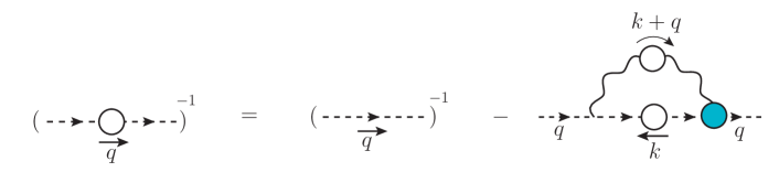
Figure 3.1: Diagrammatic representation of the ghost SDE given in Eq. (3.16). The white circles denote fully-dressed propagators, while the blue circle represents the fully-dressed ghost-gluon vertex.

Of pivotal importance for the emergence of a gluon mass scale is the SDE that determines the momentum evolution of the gluon propagator, given by

$$\Delta^{-1}(q^{2})P_{\mu\nu}(q)=q^{2}P_{\mu\nu}(q)+i{\Pi}_{\mu\nu}(q)\,,$$ (3.18)

where the gluon self-energy $\Pi_{\mu\nu}(q)$ is shown diagrammatically in the upper row of Fig. 3.2. The fully-dressed vertices entering the diagrams are determined from their own SDEs, obtaining finally a tower of coupled integral equations. It turns out that, for the purposes of this review, only the SDE governing the three-gluon vertex is required, whose diagrammatic representation is shown in the lower row of Fig. 3.2.

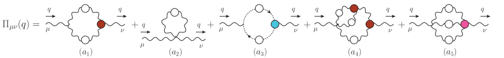
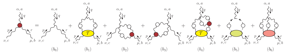
Figure 3.2: Diagrammatic representations of the gluon self-energy (top panel), $\Pi_{\mu\nu}(q)$, and three-gluon vertex (bottom panel), ${\rm{I}}\!\Gamma^{abc}_{\alpha\mu\nu}(q,r,p)$. The colored circles denote fully-dressed vertices, while the colored ellipses represent the various multiparticle scattering kernels.

An important feature of the SDEs is that one particular leg is connected to all diagrams by means of tree-level vertices; this leg corresponds precisely to the field with respect to which the action is differentiated. For example, the SDE of Fig. 3.1, whose starting point is a derivative with respect to the ghost field in Eq. (3.8), has the tree-level vertex in the ghost leg of its loop diagram. If instead we had started with a derivative with respect to the antighost field, i.e., with the master equation of (3.9), we would have obtained an SDE identical to Eq. (3.1), but with the tree-level vertex in the antighost leg. Note that these special fields couple to the various SDE diagrams through all possible classical vertices that they are part of. For instance, in the case of the SDE of the three-gluon vertex, shown in the second line of Fig. 3.2, the special field corresponds to the gluon leg carrying momentum $q$, which couples to the corresponding graphs through the three-gluon, ghost-gluon, and four-gluon classical vertices.

The SDEs must be appropriately renormalized, employing the relations given in Eq. (2.35). In general, this introduces several renormalization constants, one associated with the tree-level term, and one with each of the tree-level vertices involving the aforementioned special leg. Thus, the renormalized version of Eq. (3.16) reads

$$[D_{\!{\scriptscriptstyle R}}^{ab}(q)]^{-1}= \,Z_{c}[D^{ab}_{0}(q)]^{-1}-Z_{1}\int_{k}\Gamma_{\!0\,\mu}^{amn}(k,q,-k-q)\Delta^{\mu\nu}_{{{\scriptscriptstyle R}}\,mc}(k+q)D_{\!{\scriptscriptstyle R}}^{nd}(k){\rm{I}}\!\Gamma_{\!\!{{\scriptscriptstyle R}}\nu}^{cbd}(-r,-k,k+q)\,.$$ (3.19)

Similarly, in the more complicated case of the three-gluon SDE in Fig. 3.2, the renormalization constant $Z_{1}$ multiplies $(b_{5})$, $Z_{3}$ multiplies $(b_{0})$ and $(b_{1})$, while $Z_{4}$ multiplies $(b_{2})$, $(b_{3})$, $(b_{4})$, and $(b_{6})$.

Depending on the specific circumstances, in this work we will also employ the SDEs that arise from the $n$-PI effective action [202, 203, 204, 205, 206, 207, 208, 209, 210, 211, 116, 117], also known in the literature as “equations of motion” for the corresponding Green functions. These equations are obtained by performing additional Legendre transforms of $W[J,\eta,\bar{\eta}]$, now with respect to the full propagators and vertices.

One advantage of the $n$-PI formalism is that it treats all vertices of a given order on equal footing, leading to SDEs that are symmetric with respect to their vertex dressings, in contrast to the standard SDEs. For example, in the SDE for the three-gluon vertex derived from 3-PI at three loops, all three-point functions appear dressed in the quantum diagrams, see, e.g.,  Fig. 16.1. As a result, symmetries under the exchange of external legs, such as the Bose symmetry of the three-gluon vertex, are automatically preserved in $n$-PI truncations, whereas truncated standard SDEs need to be symmetrized by averaging over the equations derived from different legs [212, 213, 214, 215, 116, 117]. Moreover, the dressing of the tree-level vertices in the loop diagrams eliminates the aforementioned multiplicative renormalization constants; as a result, renormalization often becomes subtractive, and is rather easily implemented [216, 217, 218, 219].

4 Schwinger-Dyson equations within the PT-BFM framework

The main reason that motivates the formulation of the SDEs in the so-called PT-BFM framework is because it allows for certain crucial properties to remain intact even if certain classes of diagrams are entirely omitted. The most relevant example of such a property is the transversality of the full gluon self-energy, given in Eq. (2.32). In particular, the realization of such a fundamental result at the level of the SDE given by the diagrams of Eq. (3.2) is very complicated. In fact, already at the level of the one-loop calculation, which involves only diagrams ($d_{1}$) and ($d_{3}$), it is clear that both these diagrams must be combined for the transversality to emerge; or, in other words, neither ($d_{1}$) nor ($d_{3}$) are individually transverse. This becomes an issue when the fully-dressed diagrams are considered: in particular, one may contract each diagram by $q^{\nu}$, acting directly on the fully dressed vertices, whose STIs are triggered. It turns out that, because of the complicated ghost-related contributions [see Eqs. (2.33) and (2.34)]. Consequently, the desired result emerges only after all such contributions have been considered, and a significant amount of cancellations has taken place. Therefore, if a truncation is implemented (e.g., omission of a certain diagram, or an approximation to a fully-dressed vertex that fails to satisfy the required STI exactly), the aforementioned cancellations are typically compromised.

Quite interestingly, within the PT-BFM framework the transversality property of Eq. (2.32) is enforced in a very special way, which permits formally rigorous truncations; it is therefore important to briefly review the most salient features of this framework. In what follows we will predominantly employ the language of the BFM; for the basic principles of the PT and its connection with the BFM, the reader is referred to the extended literature on the subject [31, 37, 119, 120, 139, 111, 122].

The BFM is a powerful quantization framework, where the gauge-fixing is implemented without compromising explicit gauge invariance. Within this approach, the gauge field $A$ appearing in the classical Lagrangian density ${\cal L}_{\mathrm{cl}}$ is decomposed as $A=B+Q$, where $B$ and $Q$ are the background and quantum (fluctuating) fields, respectively. In doing so, the variable of integration in the generating functional $Z[J,\eta,\bar{\eta}]$ is the quantum field $Q$, i.e., in Eq. (2.8) we substitute $\mathcal{D}A\to\mathcal{D}Q$; moreover, $J^{a}_{\mu}A^{a\mu}\to J^{a}_{\mu}Q^{a\mu}$. The background field does not appear in loops; instead, it couples externally to the Feynman diagrams, connecting them with the asymptotic states to form S-matrix elements.

The key step in this construction is to employ the special gauge-fixing term

$${\widehat{\cal L}}_{\mathrm{gf}}=\frac{1}{2\xi_{{\scriptscriptstyle Q}}}({\widehat{D}}_{\mu}^{ab}Q^{b\mu})^{2}\,,\qquad{\widehat{D}}_{\mu}^{ab}=\partial_{\mu}\delta^{ab}+gf^{amb}B_{\mu}^{m}\,.$$ (4.1)

This choice is particularly advantageous, because it is straightforward to demonstrate that the resulting gauge-fixed action retains its invariance under gauge transformations of the background field, namely

$$\delta B^{a}_{\mu}=-g^{-1}\partial_{\mu}\theta^{a}+f^{abc}\theta^{b}B^{c}_{\mu}\,.$$ (4.2)

As a result of this invariance, when Green functions are contracted by the momentum carried by a background gluon, they satisfy Abelian (ghost-free) STIs, akin to the WTIs known from QED. In particular, denoting by $\widetilde{{\rm{I}}\!\Gamma}_{\mu\alpha\beta}(q,r,p)$, $\widetilde{{\rm{I}}\!\Gamma}_{\mu}(r,p,q)$, and $\widetilde{{\rm{I}}\!\Gamma}^{mnrs}_{\mu\alpha\beta\gamma}(q,r,p,t)$ the $BQQ$, $B{\bar{c}}c$, and $BQQQ$ vertices, respectively, we have that [37, 46, 111]

$$q^{\mu}\widetilde{{\rm{I}}\!\Gamma}_{\mu\alpha\beta}(q,r,p) = \Delta_{\alpha\beta}^{-1}(p)-\Delta_{\alpha\beta}^{-1}(r)\,,$$ (4.3)

$$q^{\mu}\widetilde{{\rm{I}}\!\Gamma}_{\mu}(r,p,q) = {D}^{-1}(p^{2})-{D}^{-1}(r^{2})\,,$$ (4.4)

$$q^{\mu}\widetilde{{\rm{I}}\!\Gamma}^{mnrs}_{\mu\alpha\beta\gamma}(q,r,p,t) = f^{mse}f^{ern}{{\rm{I}}\!\Gamma}_{\alpha\beta\gamma}(r,p,q+t)+f^{mne}f^{esr}{{\rm{I}}\!\Gamma}_{\beta\gamma\alpha}(p,t,q+r)$$ (4.5)

$$+ f^{mre}f^{ens}{{\rm{I}}\!\Gamma}_{\gamma\alpha\beta}(t,r,q+p)\,.$$

Note that the l.h.s. of these STIs involve background Green functions whilst the r.h.s. are composed exclusively by conventional Green functions.

In order to appreciate the relevance of this formalism for our purposes, consider the following two types of gluon propagators, which may be obtained by choosing appropriately the types of incoming and outgoing gluons [134]: $({\it i})$ the propagator $\langle 0|\,T\left(Q^{a}_{\mu}(q)Q^{b}_{\nu}(-q)\right)|0\rangle$, which connects two quantum gluons; this propagator coincides with the conventional gluon propagator of the covariant gauges, defined in Eq. (2.22), under the assumption that the corresponding gauge-fixing parameters, $\xi$ and $\xi_{{\scriptscriptstyle Q}}$, are identified, i.e., $\xi=\xi_{{\scriptscriptstyle Q}}$. $({\it ii})$ the propagator $\langle 0|\,T\![Q^{a}_{\mu}(q)B^{b}_{\nu}(-q)]\!|0\rangle$ that connects a $Q^{a}_{\mu}(q)$ with a $B^{b}_{\nu}(-q)$, to be denoted by $\widetilde{\Delta}^{ab}_{\mu\nu}(q)=-i\delta^{ab}\widetilde{\Delta}_{\mu\nu}(q)$. Note that since the relations expressed by Eqs. (2.22) and (3.18) apply also to $\widetilde{\Delta}_{\mu\nu}(q)$, one may define the corresponding self-energy $\widetilde{\Pi}_{\mu\nu}(q)$, as well as the function $\widetilde{\Delta}(q^{2})$.

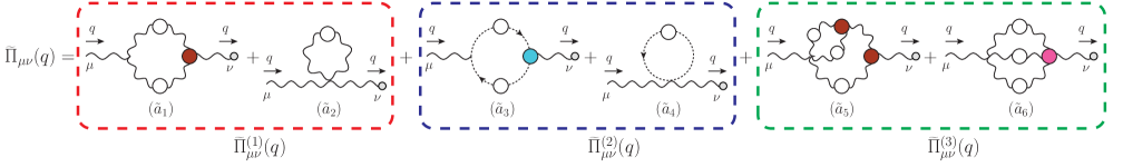
Figure 4.1: Diagrammatic representation of the $Q^{a}_{\mu}(q)B^{b}_{\nu}(-q)$ self-energy $\delta^{ab}{\widetilde{\Pi}}_{\mu\nu}(q)$; the small grey circles at the end of the gluon lines indicate a background gluon. The corresponding Feynman rules are given in Appendix B of [111].

The decisive ingredient in this discussion is the fact that the functions $\Delta(q^{2})$ and $\widetilde{\Delta}(q^{2})$ are related by the exact identity

$$\Delta(q^{2})=[1+G(q^{2})]\widetilde{\Delta}(q^{2})\,,$$ (4.6)

where $G(q^{2})$ is known as the “Batalin-Vilkovisky” (BV) function. Specifically, the $G(q^{2})$ is the $g_{\mu\nu}$ component of a certain two-point function, $\Lambda_{\mu\nu}(q)$, given by [137, 139, 220, 140, 221]

$$\Lambda_{\mu\nu}(q) = ig^{2}C_{\rm A}\int_{k}\Delta^{\rho}_{\mu}(k+q)D(k^{2})H_{\nu\rho}(-q,-k,k+q)$$ (4.7)

$$= \underbrace{G(q^{2})}_{\rm BV\,function}\!\!\!\!\!\!g_{\mu\nu}+\,L(q^{2})\,\frac{q_{\mu}q_{\nu}}{q^{2}}\,,$$

where $C_{\mathrm{A}}$ is the Casimir eigenvalue of the adjoint representation [$N$ for SU$(N)$], and $H_{\nu\mu}(r,p,q)$ denotes the ghost-gluon kernel defined in Fig. 2.2. Note that Eq. (4.6) is the simplest representative of a large class of identities, known as BQIs, relating background and quantum correlation functions, see [137, 138, 139, 111, 140].

In the Landau gauge, a special identity relates the form factors of $\Lambda_{\mu\nu}(q)$ to the ghost dressing function, $F(q^{2})$, defined in Eq. (2.24). In particular, at the level of unrenormalized quantities we have [222, 140, 71]

$$F^{-1}(q^{2})=1+G(q^{2})+L(q^{2})\,,$$ (4.8)

while, after renormalization, the identity gets modified to [99]

$$F^{-1}(q^{2})=Z_{1}[1+G(q^{2})+L(q^{2})]\,.$$ (4.9)

Note in fact that, precisely in the Landau gauge, the BV function $G(q^{2})$ coincides with the so-called Kugo–Ojima function [223, 220, 224, 225, 221].

As has been shown in [222], the dynamical equation governing $L(q^{2})$ yields $L(0)=0$, provided that the gluon propagator entering it is finite at the origin. Thus, one obtains from Eq. (4.8) the useful identity [225]

$$F^{-1}(0)=1+G(0)\,.\,$$ (4.10)

According to numerous lattice simulations and studies in the continuum (see e.g., [11, 24, 12, 226, 47, 154, 227, 228, 13, 156, 229, 230, 231, 16, 232, 167, 116, 233, 215, 234, 23]), the ghost dressing function reaches a finite (nonvanishing) value at the origin, which, due to Eq. (4.10), furnishes also the value of $G(0)$.

The final upshot of the above considerations is that one may use the BQIs in Eq. (4.6) to express the SDE given in Eq. (3.18) in terms of the $\widetilde{\Pi}_{\mu\nu}(q)$ at the modest cost of introducing the quantity $G(q^{2})$. Focusing on the former possibility, Eq. (4.6) becomes

$$\Delta^{-1}(q^{2})P_{\mu\nu}(q)=\frac{q^{2}P_{\mu\nu}(q)+i{\widetilde{\Pi}}_{\mu\nu}(q)}{1+G(q^{2})}\,,$$ (4.11)

where the diagrammatic representation of the self-energy ${\widetilde{\Pi}}_{\mu\nu}(q)$ is shown on the lower panel of Fig. 4.1.

The principal advantage of this formulation is that the self-energy ${\widetilde{\Pi}}_{\mu\nu}(q)$ contains fully-dressed vertices with a background gluon of momentum $q$ exiting from them; and these vertices satisfy Abelian STIs. In fact, the special STIs listed in Eqs. (4.3), (4.4) and (4.5) are responsible for the striking property of “block-wise” transversality  [46, 118, 134], displayed by ${\widetilde{\Pi}}_{\mu\nu}(q)$. To appreciate this point, notice that the diagrams comprising ${\widetilde{\Pi}}_{\mu\nu}(q)$ in Fig. 4.1 were separated into three different subsets (blocks), consisting of (i) one-loop dressed diagrams containing only gluons, (ii) one-loop dressed diagrams containing a ghost loop, and (iii) two-loop dressed diagrams containing only gluons. The corresponding contributions of each block to ${\widetilde{\Pi}}_{\mu\nu}(q)$ are denoted by ${\widetilde{\Pi}}^{(i)}_{\mu\nu}(q)$, with $i=1,2,3$.

The block-wise transversality is a stronger version of the standard transversality relation $q^{\mu}{\widetilde{\Pi}}_{\mu\nu}(q)=0$; it states that each block of diagrams mentioned above is individually transverse, namely

$$q^{\mu}{\widetilde{\Pi}}^{(i)}_{\mu\nu}(q)=0\,,\qquad i=1,\,2,\,3\,.$$ (4.12)

It is rather instructive to illustrate in detail how the STIs in Eqs. (4.3), (4.4) and (4.5) enforce the block-wise transversality. To that end, we will consider the cases of ${\widetilde{\Pi}}^{(1)}_{\mu\nu}(q)$ and ${\widetilde{\Pi}}^{(2)}_{\mu\nu}(q)$ ; the relevant diagrams are enclosed in the red and blue boxes of Fig. 4.1, respectively.

The diagrams $({\tilde{a}}_{1})_{\mu\nu}$ and $({\tilde{a}}_{2})_{\mu\nu}$ are given by

$$({\tilde{a}}_{1})_{\mu\nu} = \frac{1}{2}g^{2}C_{\rm A}\int_{k}\Gamma_{\!0\,\mu\alpha\beta}(q,k,-t)\Delta^{\alpha\rho}(k)\Delta^{\beta\sigma}(t)\widetilde{{\rm{I}}\!\Gamma}_{\nu\rho\sigma}(q,k,-t)$$ (4.13)

$$({\tilde{a}}_{2})_{\mu\nu} = g^{2}C_{\rm A}\int_{k}\left[\Delta_{\mu\nu}(k)-g_{\mu\nu}\Delta^{\alpha}_{\alpha}(k)\right],$$ (4.14)

where $t:=k+q$, and we have used that $\widetilde{{\rm{I}}\!\Gamma}_{\nu\sigma\rho}(-q,-k,t)=-\widetilde{{\rm{I}}\!\Gamma}_{\nu\sigma\rho}(q,k,-t)$.

The contraction of graph $({\tilde{a}}_{1})_{\mu\nu}$ by $q^{\nu}$ triggers the STI satisfied by $\widetilde{{\rm{I}}\!\Gamma}_{\mu\sigma\rho}(q,k,-t)$ [given by Eq. (4.4)], and we obtain

$$q^{\nu}({\tilde{a}}_{1})_{\mu\nu} = \frac{1}{2}g^{2}C_{\rm A}\int_{k}\Gamma_{\!0\,\mu\alpha\beta}(q,k,-t)\Delta^{\alpha\rho}(k)\Delta^{\beta\sigma}(t)\left[\Delta_{\rho\sigma}^{-1}(t)-\Delta_{\rho\sigma}^{-1}(k)\right]$$ (4.15)

$$= \frac{1}{2}g^{2}C_{\rm A}\int_{k}\Gamma_{\!0\,\mu\alpha\beta}(q,k,-t)\left[\Delta^{\alpha\beta}(k)-\Delta^{\alpha\beta}(t)\right]$$

$$= g^{2}C_{\rm A}\int_{k}\Gamma_{\!0\,\mu\alpha\beta}(q,k,-t)\Delta^{\alpha\beta}(k)$$

$$= g^{2}C_{\rm A}\int_{k}\left[q_{\mu}\Delta^{\alpha}_{\alpha}(k)-q_{\alpha}\Delta^{\alpha}_{\mu}(k)\right]\,.$$

It is clear now that the last line in Eq. (4.15) is is precisely the negative of the contraction $q^{\nu}(a_{2})_{\mu\nu}$. Hence,

$$q^{\nu}\left[({\tilde{a}}_{1})_{\mu\nu}+({\tilde{a}}_{2})_{\mu\nu}\right]=0\,\,\Longrightarrow\,\,q^{\nu}{\widetilde{\Pi}}^{(1)}_{\mu\nu}(q)=0\,.$$ (4.16)

Turning to ${\widetilde{\Pi}}^{(2)}_{\mu\nu}(q)$, consider the diagrams $({\tilde{a}}_{3})$ and $({\tilde{a}}_{4})$, given by

$$({\tilde{a}}_{3})_{\mu\nu} =g^{2}C_{\rm A}\int_{k}t_{\mu}D(t^{2})D(k^{2})\widetilde{\rm{I}}\!\Gamma_{\nu}(-k,t,-q)\,,$$ (4.17)

$$({\tilde{a}}_{4})_{\mu\nu} =g^{2}C_{\rm A}\,g_{\mu\nu}\int_{k}D(k^{2})\,.$$ (4.18)

The contraction of $({\tilde{a}}_{3})_{\mu\nu}$ by $q^{\nu}$ triggers Eq. (4.4), and so

$$q^{\nu}({\tilde{a}}_{3})_{\mu\nu} = g^{2}C_{\rm A}\int_{k}t_{\mu}D(t^{2})D(k^{2})\left[D^{-1}(k^{2})-D^{-1}(t^{2})\right]$$ (4.19)

$$= g^{2}C_{\rm A}\int_{k}t_{\mu}\left[D(t^{2})-D(k^{2})\right]$$

$$= -g^{2}C_{\rm A}\,q_{\mu}\int_{k}D(k^{2})$$

$$= -q^{\nu}({\tilde{a}}_{4})_{\mu\nu}\,.$$

Therefore,

$$q^{\nu}\left[({\tilde{a}}_{3})_{\mu\nu}+({\tilde{a}}_{4})_{\mu\nu}\right]=0\,\,\Longrightarrow\,\,q^{\nu}{\widetilde{\Pi}}^{(2)}_{\mu\nu}(q)=0\,.$$ (4.20)

Let us finally mention that the blockwise realization of the STIs appears to hold also at the level of higher Green functions; in particular, the validity of this property in the case of the vertex with three background gluons was demonstrated in [135].

5 Seagull identity and its implications

In this section we discuss an important identity, which, in conjunction with the WIs satisfied by the vertices, enforces the nonperturbative masslessness of both the photon and the gluon, in the absence of the Schwinger mechanism [95, 54].

The general idea underlying this analysis may be summarized by saying that, at the level of the SDEs, the demonstration of the masslessness of a gauge boson is fairly straightforward at the level of the $q_{\mu}q_{\nu}$ component of its self-energy, but is particularly involved when the $g_{\mu\nu}$ component is considered, requiring the non-trivial cancellation of quadratically divergent integrals.

5.1 General derivation

To proceed with the derivation of this identity, it is particularly advantageous to employ dimensional regularization. To that end, we introduce, as a concrete case of Eq. (3.17), the integral measure

$$\int_{k}:=\frac{\mu^{\epsilon}}{(2\pi)^{d}}\!\int\!\mathrm{d}^{d}k\,,$$ (5.1)

where $d=4-\epsilon$, and $\mu$ is the ’t Hooft mass.

Then, consider the class of vector functions [54]

$${\cal F}_{\mu}(k)=f(k^{2})k_{\mu}\,,$$ (5.2)

where, for the time being, $f(k^{2})$ is some arbitrary scalar function. Since ${\cal F}_{\mu}$ is an odd function of $k$, one has immediately that in dimensional regularization

$$\int_{k}{\cal F}_{\mu}(k)=0\,.$$ (5.3)

Next, impose on $f(k^{2})$ the condition originally introduced by Wilson [235], namely that, as $k^{2}\rightarrow\infty$, it vanishes sufficiently rapidly for the integral (in hyperspherical coordinates, with $y=k^{2}$)

$$\int_{k}f(k^{2})=\frac{1}{(4\pi)^{\frac{d}{2}}\Gamma\big{(}\frac{d}{2}\big{)}}\int_{0}^{\infty}\!\mathrm{d}y\,y^{\frac{d}{2}-1}f(y)$$ (5.4)

to converge for all positive values $d$ below a certain value $d^{*}$. Then, the integral is well-defined for any $d$ within $(0,d^{*})$, and can be analytically continued outside this interval.

Observe now that within dimensional regularization (or any other scheme that preserves translational invariance), one may carry out the shift $k\to k+q$ in the argument of the ${\cal F}_{\mu}(k)$ inside the integral of Eq. (5.3) without modifying the result, i.e.,

$$\int_{k}{\cal F}_{\mu}(k+q)=0\,.$$ (5.5)

Then, carrying out a Taylor expansion around $q=0$, we have

$${\cal F}_{\mu}(q+k) ={\cal F}_{\mu}(k)+q^{\nu}\bigg{\{}\frac{\partial}{\partial q^{\nu}}{\cal F}_{\mu}(q+k)\bigg{\}}_{q=0}+{\cal O}(q^{2})$$

$$={\cal F}_{\mu}(k)+q^{\nu}\frac{\partial{\cal F}_{\mu}(k)}{\partial k^{\nu}}+{\cal O}(q^{2})\,.$$ (5.6)

If we now integrate both sides of Eq. (5.6), it is clear that, in order for Eq. (5.5) to be valid, the resulting integrals must vanish order by order in $q$. Therefore, we must have

$$q^{\nu}\int_{k}\frac{\partial{\cal F}_{\mu}(k)}{\partial k^{\nu}}=0\,.$$ (5.7)

Given that this integral has two free Lorentz indices and no momentum scale, it can only be proportional to the metric tensor $g_{\mu\nu}$. In addition, since $q$ is arbitrary, one concludes that Eq. (5.7) leads to the “seagull identity”

$$\int_{k}\!\frac{\partial{\cal F}_{\mu}(k)}{\partial k_{\mu}}=0\,.$$ (5.8)

If we now use Eq. (5.2), we have that

$$\frac{\partial{\cal F}_{\mu}(k)}{\partial k_{\mu}}=2k^{2}\frac{\partial f(k^{2})}{\partial k^{2}}+df(k^{2})\,,$$ (5.9)

and Eq. (5.8) may be cast into the more standard form [95]

$$\int_{k}k^{2}\frac{\partial f(k^{2})}{\partial k^{2}}+\frac{d}{2}\int_{k}f(k^{2})=0\,.$$ (5.10)

An alternative derivation of Eq. (5.10) proceeds by carrying out a simple integration by parts in the radial part of the first integral, namely

$$\int_{0}^{\infty}\!\mathrm{d}y\,y^{\frac{d}{2}}\frac{\partial f(y)}{\partial y}=y^{\frac{d}{2}}f(y)\big{|}_{0}^{\infty}-\frac{d}{2}\int_{0}^{\infty}\!\mathrm{d}y\,y^{\frac{d}{2}-1}f(y)\,;$$ (5.11)

then, Eq. (5.10) emerges if the surface term can be dropped. At this point, an interval $(0,d^{*})$ may be found, for which the surface term indeed vanishes; then the result may be generalized through analytic continuation, for values of $d$ outside this interval, a common practice in dimensional regularization, see [141].

5.2 Spectral derivation

Quite interestingly, when $f(k^{2})=\Delta(k^{2}),D(k^{2})$, which are the cases of physical interest, the validity of Eq. (5.10) may be easily demonstrated if we assume that these functions admit the standard Källén-Lehmann representation [236, 237], [238, 239, 240, 241]

$$f(k^{2})=\int_{0}^{\infty}\!\!d\lambda^{2}\,\frac{\rho_{\!{\scriptscriptstyle f}}(\lambda^{2})}{k^{2}-\lambda^{2}}\,,\qquad f=\Delta,\,D\,,$$ (5.12)

where $\rho_{\!{\scriptscriptstyle f}}\,(\lambda^{2})$ is the spectral function (with a factor $1/\pi$ absorbed in it).

Specifically, setting

$$A(\lambda^{2}):=\int_{k}\frac{d^{d}k}{k^{2}-\lambda^{2}}\,,\qquad B(\lambda^{2}):=\int_{k}\frac{d^{d}k\,k^{2}}{(k^{2}-\lambda^{2})^{2}}\,,$$ (5.13)

employing Eq. (5.12), and using elementary algebra, we get

$$\int_{k}k^{2}\frac{\partial f(k^{2})}{\partial k^{2}}+\frac{d}{2}\int_{k}f(k^{2})=\int_{0}^{\infty}\!\!d\lambda^{2}\rho_{\!{\scriptscriptstyle f}}(\lambda^{2})\left[\omega A(\lambda^{2})-B(\lambda^{2})\right]=\int_{0}^{\infty}\!\!d\lambda^{2}\rho_{\!{\scriptscriptstyle f}}(\lambda^{2})\left\{(\omega-1)A(\lambda^{2})-\lambda^{2}\frac{dA(\lambda^{2})}{d\lambda^{2}}\right\}\,,$$ (5.14)

where we have set $\omega:=d/2$.

Then, using the text-book integral

$$A(\lambda^{2})=-i\pi^{\omega}\,\Gamma(1-\omega)\,(\lambda^{2})^{\omega-1}\,,$$ (5.15)

we have that

$$(\omega-1)A(\lambda^{2})-\lambda^{2}\frac{dA(\lambda^{2})}{d\lambda^{2}}=0\,,$$ (5.16)

making immediately evident the validity of Eq. (5.10).

5.3 Seagull cancellation in scalar QED

It is instructive to consider the action of the seagull identity in the context of a text-book gauge theory, namely scalar QED. This theory describes the interaction of a photon with a pair of charged (complex-valued) spin $0$ particles (see, e.g., [171]). There are two fundamental vertices: the vertex $-ie\Gamma_{\mu}(q,p_{1},p_{2})$, with $e$ the electric charge, corresponding to the coupling of a photon to a pair of scalars with incoming momenta $p_{1}$ and $p_{2}$, and the vertex $ie^{2}\Gamma_{\mu\nu}(q,r,p_{1},p_{2})$, connecting two photons with two scalars; at tree-level $\Gamma_{\!0\,\mu}=(p_{1}-p_{2})_{\mu}$ and $\Gamma_{\!0\,\mu\nu}=2g_{\mu\nu}$.

At the one-loop dressed level, the photon self-energy, $\Pi^{(1)}_{\mu\nu}(q)$, is given by the two diagrams shown in Fig. 5.1, i.e.,

$$\Pi^{(1)}_{\mu\nu}=(d_{1})_{\mu\nu}+(d_{2})_{\mu\nu}\,,$$ (5.17)

where

$$(d_{1})_{\mu\nu}= \,e^{2}\int_{k}(t+k)_{\mu}{\cal D}(k^{2}){\cal D}(t^{2})\Gamma_{\nu}(-q,t,-k)\,,$$

$$(d_{2})_{\mu\nu}= \,-2e^{2}g_{\mu\nu}\int_{k}{\cal D}(k^{2})\,,$$ (5.18)

with ${\cal D}(q^{2})$ standing for the fully dressed scalar propagator, and $t:=k+q$.

Figure 5.1: One-loop dressed diagrams of the photon self-energy in scalar QED. Exceptionally in this figure, dashed lines represent electrically charged scalar fields.

Importantly, the vertex $\Gamma_{\mu}(q,r,p)$ satisfies the WTI

$$q^{\mu}\Gamma_{\mu}(q,r,p)={\cal D}^{-1}(p^{2})-{\cal D}^{-1}(r^{2})\,.$$ (5.19)

Then, contracting Eq. (5.18) with $q^{\mu}$ to trigger Eq. (5.19), it is straightforward to demonstrate that $\Pi^{(1)}_{\mu\nu}(q)$ is transverse, i.e.,

$$\Pi^{(1)}_{\mu\nu}(q)=P_{\mu\nu}(q)\Pi^{(1)}(q^{2})\,.$$ (5.20)

Now, to determine $\Pi^{(1)}(0)$ we may set directly $q=0$ in Eq. (5.18). In this limit, both diagrams can only be proportional to $g_{\mu\nu}$, $(d_{i})_{\mu\nu}=g_{\mu\nu}d_{i}$, with coefficients

$$d_{1}= \,\frac{2e^{2}}{d}\int_{k}k^{\mu}{\cal D}^{2}(k^{2})\Gamma_{\mu}(0,k,-k)\,,$$

$$d_{2}= \,-2e^{2}\int_{k}{\cal D}(k^{2})\,.$$ (5.21)

At this point, the crucial assumption that the vertex $\Gamma_{\mu}(q,r,p)$ is pole-free at $q=0$, allows us to completely determine $\Gamma_{\mu}(0,k,-k)$ from the above WTI. Specifically, performing a Taylor expansion of Eq. (5.19) around $q=0$,

$$q^{\mu}\Gamma_{\mu}(0,r,-r)+{\cal O}(q^{2})=q^{\mu}\left(\frac{\partial{\cal D}^{-1}(p^{2})}{\partial q^{\mu}}\right)_{q=0}+{\cal O}(q^{2})\,,$$ (5.22)

and equating first-order coefficients, entails

$$\Gamma_{\mu}(0,r,-r)=\frac{\partial{\cal D}^{-1}(r^{2})}{\partial r^{\mu}}\,,$$ (5.23)

which is the well-known WI of scalar QED.

Then, using Eq. (5.23) into Eq. (5.21), the coefficient $d_{1}$ reduces to

$$d_{1}=-\frac{2e^{2}}{d}\int_{k}k^{\mu}\frac{\partial{\cal D}(k^{2})}{\partial k^{\mu}}=-\frac{4e^{2}}{d}\int_{k}k^{2}\frac{\partial{\cal D}(k^{2})}{\partial k^{2}}\,.$$ (5.24)

Hence, combining the above with $d_{2}$ of Eq. (5.21),

$$\Pi^{(1)}(0)=-\frac{4e^{2}}{d}\underbrace{\left[\int_{k}k^{2}\frac{\partial{\cal D}(k^{2})}{\partial k^{2}}+\frac{d}{2}\int_{k}{\cal D}(k^{2})\right]}_{\text{seagull identity}}\,.$$ (5.25)

Finally, we recognize that the term in brackets in Eq. (5.25) is precisely the seagull identity of Eq. (5.10), with $f(k^{2})={\cal D}(k^{2})$. Therefore, $\Pi^{(1)}(0)=0$.

5.4 Masslessness of the photon

Particularly interesting is the action of the seagull identity at the level of standard QED₄, leading to a concise proof of the exact masslessness of the physical photon, in the absence of the Schwinger mechanism.

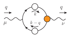
Figure 5.2: The full photon self-energy in QED₄.

The full photon self-energy, $\Pi_{\mu\nu}(q)$, is given by the single diagram shown in Fig. 5.2, which captures all possible quantum effects, both perturbative and non-perturbative. In particular, $\Pi_{\mu\nu}(q)$ is given by

$$\Pi_{\mu\nu}(q)=-e^{2}\int_{k}{\rm Tr}\left[\gamma_{\mu}S(k)\Gamma_{\nu}(-q,k,q-k)S(k-q)\right]\,,$$ (5.26)

where $\Gamma_{\nu}$ is the fully-dressed electron-photon vertex, which satisfies the WTI

$$q^{\mu}\Gamma_{\mu}(q,k,-k-q)=S^{-1}(k+q)-S^{-1}(k)\,\,\,\,\Longrightarrow\,\,\,\Gamma_{\mu}(0,k,-k)=\frac{\partial{S}^{-1}(k)}{\partial k^{\mu}}=-{S}^{-1}(k)\frac{\partial S(k)}{\partial k^{\mu}}{S}^{-1}(k)\,.$$ (5.27)

At this point one may set $q=0$ directly into Eq. (5.26), thus isolating the $g_{\mu\nu}$ component, exactly as was done in the scalar QED case; it is instructive, however, to reach the same result by exploiting the transversality of $\Pi_{\mu\nu}(q)$, for arbitrary values of $q^{2}$. Specifically, the transversality of $\Pi_{\mu\nu}(q)$ follows directly from the QED analogue of Eq. (2.32); or, it may be derived directly from Eq. (5.26) by contacting with $q^{\nu}$ and appealing to the first relation in Eq. (5.27). Therefore, we may set $\Pi_{\mu\nu}(q)=P_{\mu\nu}(q)\,\Pi(q)$ on the l.h.s. of Eq. (5.26), and obtain an expression for $\Pi(q)$ by contracting both sides by $g^{\mu}_{\nu}$, and using $P_{\mu}^{\mu}(q)=d-1$. Thus, we obtain

$$\Pi(q^{2})=-\frac{e^{2}}{d-1}\int_{k}{\rm Tr}\left[\gamma^{\mu}S(k)\Gamma_{\mu}(-q,k,q-k)S(k-q)\right]\,.$$ (5.28)

Then, setting $q=0$ into Eq. (5.28), suppressing prefactors, and employing the second relation in Eq. (5.27), we have,

$$\Pi(0)\sim\int_{k}{\rm Tr}\left[\gamma^{\mu}S(k)\Gamma_{\mu}(0,k,-k)S(k)\right]\sim\int_{k}{\rm Tr}\left[\gamma^{\mu}\frac{\partial S(k)}{\partial k^{\mu}}\right]\,.$$ (5.29)

Using that the most general form of $S(k)$ is given by $S(k)=a(k^{2})\not{k}+b(k^{2})$ we have that

$$\frac{\partial S(k)}{\partial k^{\mu}}=\frac{\partial a(k^{2})}{\partial k^{\mu}}\not{k}+a(k^{2})\gamma_{\mu}+\frac{\partial b(k^{2})}{\partial k^{\mu}}=2k_{\mu}\frac{\partial a(k^{2})}{\partial k^{2}}\not{k}+a(k^{2})\gamma_{\mu}+2k_{\mu}\frac{\partial b(k^{2})}{\partial k^{2}}\,.$$ (5.30)

Substituting the above expression into Eq. (5.29), we see that, since ${\rm Tr}\gamma_{\mu}=0$, the third term drops out, and one gets

$$\Pi(0) \sim 2\int_{k}k_{\mu}k_{\nu}\frac{\partial a(k^{2})}{\partial k^{2}}{\rm Tr}\underbrace{[\gamma^{\mu}\gamma^{\nu}]}_{dg^{\mu\nu}}\,\,+\,\,\int_{k}a(k^{2}){\rm Tr}\underbrace{[\gamma^{\mu}\gamma_{\mu}]}_{d^{2}}$$ (5.31)

$$\sim 2d\underbrace{\left[\int_{k}k^{2}\frac{\partial a(k^{2})}{\partial k^{2}}+\frac{d}{2}\int_{k}a(k^{2})\right]}_{\text{seagull identity}}=0\,,$$

establishing the exact masslessness of the photon within standard QED. Note finally that, contrary to what happens in the scalar QED example and in the Yang-Mills case (next subsection), in QED₄ the seagull identity emerges in its entirety from the single diagram shown in Fig. 5.2.

5.5 Seagull cancellations in QCD

In the absence of the Schwinger mechanism, the seagull identity would also imply the masslessness of the gluon, as we now demonstrate. For simplicity, we will consider only the one-loop dressed diagrams, ${\widetilde{\Pi}}^{(1)}_{\mu\nu}(q)$ and ${\widetilde{\Pi}}^{(2)}_{\mu\nu}(q)$, of Fig. 4.1; the detailed analysis of ${\widetilde{\Pi}}^{(3)}_{\mu\nu}(q)$ is given in [54]. In the first version of the proof we will keep the value of the gauge-fixing parameter $\xi$ in the gluon propagators general, while in the second, given in App. C, we will discuss certain technical issues related to the implementation of the Landau gauge.

By virtue of the Abelian STIs satisfied by the BFM vertices, the analysis of ${\widetilde{\Pi}}^{(1)}_{\mu\nu}(q)$ is completely analogous to the case of scalar QED in Eq. (5.3). We begin by setting $q=0$ in the expression for $({\tilde{a}}_{1})_{\mu\nu}$ given by Eq. (4.13), denoting the result by ${\tilde{a}}_{1\mu\nu}$; we have

$${\tilde{a}}_{1\mu\nu}= \,\frac{1}{2}g^{2}C_{\rm A}\int_{k}\Gamma_{\!0\,\mu\alpha\beta}(0,k,-k)\Delta^{\alpha\rho}(k)\Delta^{\beta\sigma}(k)\widetilde{\Gamma}_{\nu\rho\sigma}(0,k,-k)\,,$$ (5.32)

where

$$\Gamma_{\!0\,\mu\alpha\beta}(0,k,-k)=2k_{\mu}g_{\alpha\beta}-k_{\alpha}g_{\mu\beta}-k_{\beta}g_{\mu\alpha}\,.$$ (5.33)

On the other hand, $({\tilde{a}}_{2})_{\mu\nu}$ remains unchanged, $({\tilde{a}}_{2})_{\mu\nu}={\tilde{a}}_{2\mu\nu}$. Since both contributions are proportional to $g_{\mu\nu}$, we set (${\tilde{a}}_{1})_{\mu\nu}={\tilde{a}}_{1}g_{\mu\nu}$ and $({\tilde{a}}_{2})_{\mu\nu}={\tilde{a}}_{2}g_{\mu\nu}$, with

$${\tilde{a}}_{1}= \,\frac{g^{2}C_{\rm A}}{2d}\int_{k}\Gamma_{\!0\,\mu\alpha\beta}(0,k,-k)\Delta^{\alpha\rho}(k)\Delta^{\beta\sigma}(k)\widetilde{\Gamma}^{\mu}_{\rho\sigma}(0,k,-k)\,,$$ (5.34)

$${\tilde{a}}_{2}= \,-g^{2}C_{\rm A}\frac{(d-1)}{d}\int_{k}\Delta^{\alpha}_{\alpha}(k)\,.$$ (5.35)

Now, assuming that the vertex $\widetilde{\Gamma}_{\alpha\mu\nu}(q,r,p)$ is pole-free at $q=0$ (i.e., no Schwinger mechanism), the Taylor expansion of the Abelian STI of Eq. (4.4) yields the WI,

$$\widetilde{\Gamma}_{\alpha\mu\nu}(0,r,-r)=\frac{\partial\Delta_{\mu\nu}^{-1}(r)}{\partial r^{\alpha}}\,.$$ (5.36)

Note that the above formula is valid also at tree level, due to the fact that $\widetilde{\Gamma}_{\!0\,\alpha\mu\nu}$ depends on $\xi_{Q}$, i.e.,

$$\widetilde{\Gamma}_{\!0\,\alpha\mu\nu}(q,r,p)=(q-r)_{\nu}g_{\alpha\mu}+(r-p)_{\alpha}g_{\mu\nu}+(p-q)_{\mu}g_{\nu\alpha}+\xi_{Q}^{-1}(g_{\alpha\nu}r_{\mu}-g_{\alpha\mu}p_{\nu})\,.$$ (5.37)

Combining the above with Eq. (5.34), and noting that

$$\Delta^{\alpha\rho}(k)\Delta^{\beta\sigma}(k)\frac{\partial\Delta^{-1}_{\rho\sigma}(k)}{\partial k_{\mu}}=-\frac{\partial\Delta^{\alpha\beta}(k)}{\partial k_{\mu}}\,,$$ (5.38)

we obtain

$${\tilde{a}}_{1}= \,-\frac{g^{2}C_{\rm A}}{2d}\int_{k}\Gamma_{\!0\,\mu\alpha\beta}(0,k,-k)\frac{\partial\Delta^{\alpha\beta}(k)}{\partial k_{\mu}}$$

$$= \,-\frac{g^{2}C_{\rm A}}{2d}\left\{\int_{k}\frac{\partial[\Delta^{\alpha\beta}(k)\Gamma_{\!0\,\mu\alpha\beta}(0,k,-k)]}{\partial k_{\mu}}-\int_{k}\Delta^{\alpha\beta}(k)\frac{\partial\Gamma_{\!0\,\mu\alpha\beta}(0,k,-k)}{\partial k_{\mu}}\right\}\,,$$ (5.39)

where an integration by parts was performed to obtain the last line.

At this point, it is straightforward to show that

$$\Delta^{\alpha\beta}(k)\Gamma_{\!0\,\mu\alpha\beta}(0,k,-k)=2(d-1)k_{\mu}\Delta(k^{2})\,,\qquad\frac{\partial\Gamma_{\!0\,\mu\alpha\beta}(0,k,-k)}{\partial k_{\mu}}=2(d-1)g_{\alpha\beta}\,,$$ (5.40)

such that

$${\tilde{a}}_{1}=g^{2}C_{\rm A}\frac{(d-1)}{d}\int_{k}\Delta^{\alpha}_{\alpha}(k)-g^{2}C_{\rm A}\frac{(d-1)}{d}\int_{k}\frac{{\cal F}_{\mu}(k)}{\partial k_{\mu}}\,,$$ (5.41)

where

$${\cal F}_{\mu}(k):=k_{\mu}\Delta(k^{2})\,.$$ (5.42)

Finally, combining Eqs. (5.41) and (5.35), yields

$${\widetilde{\Pi}}^{(1)}(0)={\tilde{a}}_{1}+{\tilde{a}}_{2}=-g^{2}C_{\rm A}\frac{(d-1)}{d}\underbrace{\int_{k}\frac{{\cal F}_{\mu}(k)}{\partial k_{\mu}}}_{\text{seagull identity}}=0\,,$$ (5.43)

where we used the compact version of the seagull identity given by Eq. (5.8).

We next turn to the ghost-loop diagrams ${\tilde{a}}_{3}$ and ${\tilde{a}}_{4}$ in Fig. 4.1, which comprise ${\widetilde{\Pi}}^{(2)}_{\mu\nu}(q)$; their expressions for general $q$ are given in Eq. (4.18). Evidently, graph ${\tilde{a}}_{3}$ is $q$-independent, and directly proportional to $g_{\mu\nu}$. As for ${\tilde{a}}_{3}$, after setting $q=0$ in the corresponding expression in Eq. (4.18), the result also depends on $g_{\mu\nu}$ alone. Specifically, we obtain

$${\tilde{a}}_{3}= \,\frac{g^{2}C_{\rm A}}{d}\int_{k}k_{\mu}D^{2}(k^{2})\widetilde{\rm{I}}\!\Gamma^{\mu}(-k,k,0)\,,$$

$${\tilde{a}}_{4}= \,g^{2}C_{\rm A}\int_{k}D(k^{2})\,.$$ (5.44)

Then, if the ghost-gluon vertex ${\widetilde{\Gamma}}_{\alpha}(r,p,q)$ is pole-free, the Taylor expansion of Eq. (4.4) leads to the WI

$${\widetilde{\Gamma}}_{\alpha}(r,-r,0)=\frac{\partial D^{-1}(r^{2})}{\partial r^{\alpha}}=2r_{\alpha}\frac{\partial D^{-1}(r^{2})}{\partial r^{2}}\,,$$ (5.45)

which, when substituted into Eq. (5.44) (with $r\to-k$), yields

$${\tilde{a}}_{3}=\frac{2g^{2}C_{\rm A}}{d}\int_{k}k^{2}\frac{\partial D(k^{2})}{\partial k^{2}}\,.$$ (5.46)

Hence, combining Eqs. (5.44) and (5.46),

$${\widetilde{\Pi}}^{(2)}(0)={\tilde{a}}_{3}+{\tilde{a}}_{4}=\frac{2g^{2}C_{\rm A}}{d}\underbrace{\left[\int_{k}k^{2}\frac{\partial D(k^{2})}{\partial k^{2}}+\frac{d}{2}\int_{k}D(k^{2})\right]}_{\text{seagull identity}}=0\,,$$ (5.47)

where we have used the version of the seagull identity given in Eq. (5.10).

Note that this demonstration does not assume any particular form for the gluon propagator, $\Delta(q^{2})$. In fact, quite interestingly, even if the gluon propagator were to be made massive by hand, the seagull identity would require that mass to vanish [54].

6 Schwinger mechanism in QCD: general notions

Schwinger’s fundamental observation on gauge invariance and vector meson mass [90, 91] may be summarized in a modern language as follows: If the dimensionless vacuum polarization of the vector meson develops a pole with positive residue at zero momentum transfer, then the vector meson acquires a mass, even if the gauge symmetry forbids a mass term at the level of the fundamental Lagrangian.

To see in some detail how this general idea is realized, it is convenient to introduce precisely the dimensionless vacuum polarization mentioned by Schwinger; we will denote this function by ${\bf\Pi}(q^{2})$, and define it as $\Pi(q^{2})=q^{2}{\bf\Pi}(q^{2})$. Then, from the second relation of Eq. (2.22), written in Euclidean space, we have that $\Delta^{-1}(q^{2})=q^{2}[1+{\bf\Pi}(q^{2})]$.

Then, the Schwinger condition that at zero momentum transfer ${\bf\Pi}(q^{2})$ develops a pole with a positive residue, $c^{2}$, means that

$$\lim_{q^{2}\to 0}{\bf\Pi}(q^{2})=c^{2}/q^{2}\,.$$ (6.1)

In what follows we will refer to this type of pole as a massless pole or a Schwinger pole.

Evidently, if Eq. (6.1) holds, then

$$\,\,\lim_{q^{2}\to 0}\,\Delta^{-1}(q^{2})=\lim_{q^{2}\to 0}\,(q^{2}+c^{2})\,\,\Longrightarrow\,\,\,\Delta^{-1}(0)=c^{2}\,,$$ (6.2)

where the residue of the pole acts as the effective squared mass, $m^{2}$, of the vector meson, e.g., one carries out the identification $c^{2}=m^{2}$. It is important to emphasize that in the absence of interactions the vector meson (or gauge boson) remains massless, since $g=0$ implies ${\bf\Pi}(q^{2})=0$.

The most celebrated example where this mechanism was first showcased is the so-called “Schwinger model”, namely QED₂ with massless fermions [91, 242, 243]. Due to the particularities of the two-dimensional Dirac matrices, the one-loop vacuum polarization diagram (i.e., Fig. 5.2 with all its components set to their tree-level values) is the only possible quantum correction that the photon propagator may receive. Then, an elementary calculation shows that the photon acquires a mass, given by the exact formula $m^{2}_{\gamma}=e^{2}/\pi$, where $e$ is the dimensionful electric charge in $d=2$.

It is important to emphasize that the standard Higgs mechanism is a very special case of the Schwinger mechanism. In particular, in this case the gauge boson mass, $M$, is given by $M=gv/2$, where $v$ is the vacuum expectation value of a fundamental scalar field $\phi$; evidently, the gauge boson mass vanishes when the gauge coupling is set to zero. Since the Euclidean gauge boson propagator becomes

$$\Delta^{-1}(q^{2})=q^{2}+M^{2}=q^{2}\left(1+\frac{g^{2}v^{2}}{4q^{2}}\right)\,,$$ (6.3)

it is clear that, in the terminology of the Schwinger mechanism, the square of the vacuum expectation value of the scalar field plays the role of the residue of the pole. Note, in addition, a pivotal physical difference between the Higgs mechanism and the Schwinger mechanism taking place in QCD: while the Higgs mechanism is accompanied by a fundamental scalar excitations, namely the Higgs boson, the QCD spectrum remains completely unaffected by the action of the Schwinger mechanism.

Turning to Yang-Mills theories in $d=4$, and in particular QCD, the natural question that arises is what makes the gluon vacuum polarization function ${\bf\Pi}(q^{2})$ exhibit massless poles, given the absence of elementary scalar fields. The starting observation for addressing this question is that the fully-dressed vertices of the theory generate massless scalar excitations dynamically. In particular, the required Schwinger poles arise as composite bound state excitations, produced through the fusion of two gluons or of a ghost-antighost pair into a color-carrying scalar, $\Phi^{a}$, of vanishing mass [92, 93, 142, 31, 143, 96, 97, 98, 144, 145, 146]. Evidently, since these excitations carry color, they do not appear as observable states. The formation of these states is controlled by special BSEs; it may be understood as the limiting case of the production of a bound state whose mass shrinks to zero when the theory becomes sufficiently strongly coupled, as is the case of QCD. Given that the fully-dressed vertices enter in the diagrammatic expansion of the gluon self-energy (see Fig. 3.2), their poles are finally transmitted to ${\bf\Pi}(q^{2})$, giving rise to Eq. (6.1), and through it to an effective mass scale for the gluon [31, 46, 47, 77, 99].

In what follows we will elaborate in detail on two main aspects associated with the realization of the Schwinger mechanism in QCD. First, we will show how the emergence of massless poles in the fundamental vertices gives rise to a gluon mass, namely the way that the key sequence captured by Eqs. (6.1) and (6.2) proceeds within the intricate structure of the gauge sector of QCD. Second, we will address the equally fundamental issue of identifying the precise dynamics that drive the appearance of Schwinger poles in the vertices.

7 Fundamental QCD vertices with Schwinger poles

The implementation of the Schwinger mechanism in QCD is intimately connected with the appearance of special irregularities in the fundamental vertices of the theory, namely of poles that manifest themselves as the incoming momenta tend to zero. In what follows we will consider the pole structure of two of the QCD vertices, namely the three-gluon and ghost-gluon vertices, ${\rm{I}}\!\Gamma_{\alpha\mu\nu}(q,r,p)$ and ${\rm{I}}\!\Gamma_{\alpha}(r,p,q)$, respectively, introduced in Section 2. The four-gluon and quark-gluon vertices also develop such poles [54, 170], but their overall impact is rather limited, and will be therefore omitted in what follows.

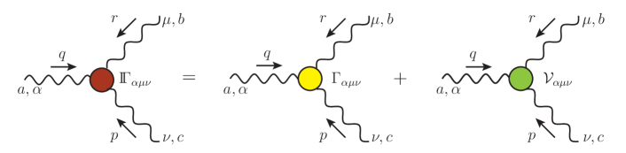
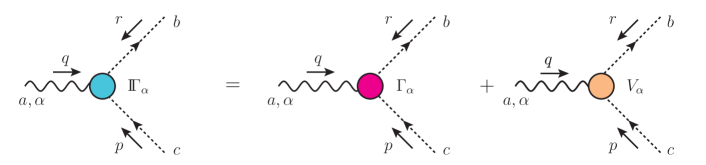
Figure 7.1: The diagrammatic representation of the three-gluon and ghost-gluon vertices introduced in Eqs. (7.1) and (7.2): ${\rm{I}}\!\Gamma_{\alpha\mu\nu}(q,r,p)$ (first row) and ${\rm{I}}\!\Gamma_{\alpha}(r,p,q)$ (second row). The first term on the r.h.s. indicates the pole-free part, $\Gamma_{\alpha\mu\nu}(q,r,p)$ or $\Gamma_{\alpha}(r,p,q)$, while the second denotes the pole term ${\cal V}_{\alpha\mu\nu}(q,r,p)$ or $V_{\alpha}(r,p,q)$.

Given the key role played by the massless poles, it is natural at this point to separate each vertex ${\rm{I}}\!\Gamma$ into two parts, as shown in Fig. 7.1: the pole-free part, denoted by $\Gamma$, and the part that carries the Schwinger poles, denoted by $V$. In particular, for the three-gluon and ghost-gluon vertices, we write

$${\rm{I}}\!\Gamma_{\alpha\mu\nu}(q,r,p)=\Gamma_{\alpha\mu\nu}(q,r,p)+{\cal V}_{\alpha\mu\nu}(q,r,p)\,,$$ (7.1)

and

$${\rm{I}}\!\Gamma_{\alpha}(r,p,q)=\Gamma_{\alpha}(r,p,q)+V_{\alpha}(r,p,q)\,.$$ (7.2)

A crucial restriction on the general form of ${\cal V}_{\alpha\mu\nu}(q,r,p)$ and $V_{\alpha}(r,p,q)$ arises from the requirement that the massless poles be longitudinally coupled. This means that poles in $q^{2}$, $r^{2}$, or $p^{2}$ must be multiplied by $q^{\alpha}$, $r^{\mu}$, or $p^{\nu}$, respectively. Similarly, double poles are accompanied by two such momenta; for example, the double pole $1/q^{2}r^{2}$, is multiplied by $q^{\alpha}r^{\mu}$.

The physical reason for imposing this requirement is that, in this way, the absence of strong divergences in physical quantities, such as S-matrix elements, is guaranteed. Indeed, the longitudinal nature of ${\cal V}_{\alpha\mu\nu}(q,r,p)$ and $V_{\mu}(r,p,q)$ annihilates them when they get contracted by external conserved currents, or, equivalently, when they trigger the equations of motion (EoM) of the external particles. For instance, for the three-gluon vertex in Fig. 7.2, we have that ($q=p_{1}-p_{2}$)

$$q^{\alpha}\gamma_{\alpha}=\not{q}=(\underbrace{\not{p}_{1}-m}_{{\rm EoM}})-(\underbrace{\not{p}_{2}-m}_{{\rm EoM}})=0\,,$$ (7.3)

and similarly for the other two legs. Equivalently, one may say that ${\cal V}_{\alpha\mu\nu}$ must be annihilated when all its legs are contracted by the corresponding projection tensors, namely [see Fig. 7.2]

$$P^{\alpha^{\prime}}_{\alpha}(q)P^{\mu^{\prime}}_{\mu}(r)P^{\nu^{\prime}}_{\nu}(p){\cal V}_{\alpha^{\prime}\mu^{\prime}\nu^{\prime}}(q,r,p)=0\,,$$ (7.4)

and

$$P^{\alpha^{\prime}}_{\alpha}(q)V_{\alpha^{\prime}}(r,p,q)=0\,.$$ (7.5)

It is particularly important to emphasize that the longitudinal nature of the Schwinger poles is automatically enforced within the bound state scenario presented in Sec. 14.

Figure 7.2: Cancellation of longitudinally coupled poles when contracted with conserved currents.

It is especially instructive to illustrate how non-longitudinal poles would induce divergences to certain combinations of vertex form factors, which are known from lattice simulations to be completely divergence-free.

To appreciate this point, consider the ghost-gluon vertex, ${\rm{I}}\!\Gamma_{\alpha}(r,p,q)$. The tensorial decomposition of $\Gamma_{\alpha}$ is given by

$$\Gamma_{\alpha}(r,p,q)=r_{\alpha}B_{1}(r,p,q)+q_{\alpha}B_{2}(r,p,q)\,,$$ (7.6)

and if no restriction is imposed on the tensor structure of $V_{\alpha}(r,p,q)$, we have

$$V_{\alpha}(r,p,q)=\frac{1}{q^{2}}\left[r_{\alpha}C_{1}(r,p,q)+q_{\alpha}C_{2}(r,p,q)\right]\,.$$ (7.7)

Now, after amputating the external legs, the typical lattice “observable” associated with the Landau-gauge ghost-gluon vertex has the form [244, 11, 245, 246]

$$L_{\rm{gh}}(r,p,q)=\frac{\Gamma_{\!0\,\alpha}(r,p,q)P^{\alpha\alpha^{\prime}}(q){\rm{I}}\!\Gamma_{\alpha^{\prime}}(r,p,q)}{\Gamma_{\!0\,\alpha}(r,p,q)P^{\alpha\alpha^{\prime}}(q)\Gamma_{\!0\,\alpha^{\prime}}(r,p,q)}=\frac{\left[q^{2}r^{\alpha^{\prime}}-(q\cdot r)q^{\alpha^{\prime}}\right]{\rm{I}}\!\Gamma_{\alpha^{\prime}}(r,p,q)}{q^{2}r^{2}-(q\cdot r)^{2}}\,.$$ (7.8)

Then, assuming the general tensor structures of Eqs. (7.6) and (7.7), we have

$$L_{\rm{gh}}(r,p,q)=B_{1}(r,p,q)+\frac{1}{q^{2}}C_{1}(r,p,q)\,.$$ (7.9)

Hence, $L_{\rm{gh}}(r,p,q)$ would contain a pole at $q=0$, which, however, is not observed in the available lattice data. Thus, $C_{1}(r,p,q)$ must be vanishing sufficiently fast in the limit $q\to 0$ for the pole to become evitable, or, equivalently, to be absorbed into a redefinition of the $B_{2}(r,p,q)$ in Eq. (7.6).

Therefore, $V_{\alpha}(r,p,q)$ is strictly longitudinal, in which case we can drop the index “2” in $C_{2}(r,p,q)$ and write simply

$$V_{\alpha}(r,p,q)=\frac{q_{\alpha}}{q^{2}}C(r,p,q)\,.$$ (7.10)

An analogous conclusion can be reached for the three-gluon vertex, whose typical lattice observables in Landau gauge have the form [244, 188, 189, 247, 190, 23, 248, 249, 250, 251, 252]

$$L_{i}(r,p,q)=\frac{\lambda^{i}_{\alpha\mu\nu}(q,r,p)P^{\alpha\alpha^{\prime}}(q)P^{\mu\mu^{\prime}}(r)P^{\nu\nu^{\prime}}(p){\rm{I}}\!\Gamma_{\alpha^{\prime}\mu^{\prime}\nu^{\prime}}(q,r,p)}{\Gamma_{\!0\,\alpha\mu\nu}(q,r,p)P^{\alpha\alpha^{\prime}}(q)P^{\mu\mu^{\prime}}(r)P^{\nu\nu^{\prime}}(p)\Gamma_{\!0\,\alpha^{\prime}\mu^{\prime}\nu^{\prime}}(q,r,p)}\,,$$ (7.11)

where the $\lambda_{\alpha\mu\nu}^{i}(q,r,p)$ are suitable projectors that isolate specific form factors or linear combinations thereof. Then, the condition of Eq. (7.4) is tantamount to the absence of poles in the lattice functions $L_{i}(r,p,q)$.

The most general form of ${\cal V}_{\alpha\mu\nu}(q,r,p)$ consistent with the condition that all poles are longitudinally coupled is given by [149]

$${\cal V}_{\alpha\mu\nu}(q,r,p) =\frac{q_{\alpha}}{q^{2}}\left(g_{\mu\nu}V_{1}+p_{\mu}r_{\nu}V_{2}\right)\,\,+\,\,\frac{r_{\mu}}{r^{2}}\left(g_{\alpha\nu}V_{3}+q_{\nu}p_{\alpha}V_{4}\right)\,\,+\,\,\frac{p_{\nu}}{p^{2}}\left(g_{\alpha\mu}V_{5}+r_{\alpha}q_{\mu}V_{6}\right)$$

$$+\frac{q_{\alpha}r_{\mu}}{q^{2}r^{2}}(q-r)_{\nu}V_{7}\,\,+\,\,\frac{r_{\mu}p_{\nu}}{r^{2}p^{2}}(r-p)_{\alpha}V_{8}\,+\frac{p_{\nu}q_{\alpha}}{p^{2}q^{2}}(p-q)_{\mu}V_{9}\,\,+\,\,\frac{q_{\alpha}r_{\mu}p_{\nu}}{q^{2}r^{2}p^{2}}\,V_{10}\,,$$ (7.12)

where $V_{i}\equiv V_{i}(q,r,p)$. Note that Bose symmetry imposes that the $V_{i}$ have definite transformation properties under the interchange of momenta [see Eqs. (13.11) and (13.12)].

The Bose symmetry of the three-gluon vertex guarantees the presence of Schwinger poles in all three momenta, $q$, $r$, and $p$, of the vertex ${\cal V}_{\alpha\mu\nu}(q,r,p)$. Out of these three possibilities, the pole directly responsible for the emergence of a gluon mass scale is the one that carries the external momentum of the gluon SDE, denoted by $q$ in diagrams ($a_{1}$) of Fig. 3.2. In fact, due to their longitudinal nature, the poles in the other channels get annihilated when contracted by the internal Landau-gauge propagators of ($a_{1}$).

The latter observation motivates us to isolate the part of ${\cal V}_{\alpha\mu\nu}(q,r,p)$ that contains only a single pole in $q$, and denote it by $V_{\alpha\mu\nu}(q,r,p)$. Thus, we have

$${\cal V}_{\alpha\mu\nu}(q,r,p)=V_{\alpha\mu\nu}(q,r,p)+\cdots\,,\qquad V_{\alpha\mu\nu}(q,r,p)=\frac{q_{\alpha}}{q^{2}}C_{\mu\nu}(q,r,p)\,,$$ (7.13)

where the ellipsis indicate terms with at least one pole in the $p$ or $r$ channel, while $C_{\mu\nu}(q,r,p)$ is pole-free.

Now, the most general tensor structure of $C_{\mu\nu}(q,r,p)$ is given by [96, 97, 54]

$$C_{\mu\nu}(q,r,p)=g_{\mu\nu}V_{1}(q,r,p)+p_{\mu}r_{\nu}V_{2}(q,r,p)+r_{\mu}r_{\nu}C_{3}(q,r,p)+p_{\mu}p_{\nu}C_{4}(q,r,p)+r_{\mu}p_{\nu}C_{5}(q,r,p)\,,$$ (7.14)

where the direct comparison between Eqs. (7.13) and (7.12) allowed us to unambiguously identify the $g_{\mu\nu}$ and $p_{\mu}r_{\nu}$ form factors as $V_{1}(q,r,p)$ and $V_{2}(q,r,p)$, respectively.

Relating the $C_{i}$ for $i=3,\,4,\,5$ with the $V_{j}$ is more subtle. In particular, the $C_{i}$ are comprised by contributions of order $r^{2}$ and/or $p^{2}$ contained inside the $V_{i}$, with $i=7\,,9\,,10$; when inserted in Eq. (7.12), these terms furnish poles in $q$ only. For instance, performing a Taylor expansion of $V_{7}(q,r,p)$ around $r=0$,

$$\frac{V_{7}(q,r,p)}{q^{2}r^{2}}=\frac{V_{7}(q,0,-q)}{q^{2}r^{2}}+\frac{2(q\cdot r)}{q^{2}r^{2}}\left[\frac{\partial V_{7}(q,r,p)}{\partial p^{2}}\right]_{r=0}+\frac{1}{q^{2}}\left[\frac{\partial V_{7}(q,r,p)}{\partial r^{2}}\right]_{r=0}+\ldots\,,$$ (7.15)

the last term contains a pole only in $q$. Hence, matching tensor structures in Eqs. (7.13) and (7.12), yields

$$C_{3}(q,r,p)=-2\left[\frac{\partial V_{7}(q,r,p)}{\partial r^{2}}\right]_{r=0}+\ldots\,,$$ (7.16)

with ellipsis indicating contributions from $V_{7}(q,r,p)$, $V_{10}(q,r,p)$, and higher derivatives of $V_{7}(q,r,p)$.

When ${\rm{I}}\!\Gamma_{\alpha\mu\nu}(q,r,p)$ is contracted by two internal propagators in the Landau gauge [as happens in graph ($a_{1}$) of Fig. 3.2], it suffices to consider

$$P^{\mu^{\prime}}_{\mu}(r)P^{\nu^{\prime}}_{\nu}(p){\cal V}_{\alpha\mu\nu}(q,r,p)=P^{\mu^{\prime}}_{\mu}(r)P^{\nu^{\prime}}_{\nu}(p)V_{\alpha\mu^{\prime}\nu^{\prime}}(q,r,p)\,.$$ (7.17)

In this case, only the form factor $V_{1}$ and $V_{2}$ are relevant, since

$$P^{\mu^{\prime}}_{\mu}(r)P^{\nu^{\prime}}_{\nu}(p)C_{\mu^{\prime}\nu^{\prime}}(q,r,p)= \,P^{\rho}_{\mu}(r)P_{\nu\rho}(p)V_{1}(q,r,p)+q_{\mu^{\prime}}q_{\nu^{\prime}}P^{\mu^{\prime}}_{\mu}(r)P^{\nu^{\prime}}_{\nu}(p)V_{2}(q,r,p)\,,$$ (7.18)

where momentum conservation was used in passing from Eq. (7.14) to Eq. (7.18).

Note that, from the Bose symmetry of the full vertex,

$$V_{1}(q,r,p)=-V_{1}(q,p,r)\,,\Longrightarrow V_{1}(0,r,-r)=0\,;$$ (7.19)

the same result follows straightforwardly from the STI of Eq. (2.33), as we show in Sec. 11. Hence, performing a Taylor expansion around $q=0$,

$$V_{1}(q,r,p)=2(q\cdot r){\mathbb{C}}(r^{2})\,,\qquad{\mathbb{C}}(r^{2}):=\left[\frac{\partial V_{1}(q,r,p)}{\partial p^{2}}\right]_{q=0}\,.$$ (7.20)

A result analogous to Eq. (7.19) can be shown for the pole term, $C(r,p,q)$, of the ghost-gluon vertex (see App. E), namely

$$C(r,-r,0)=0\,,$$ (7.21)

which implies

$$C(r,p,q)=2(q\cdot r){\mathcal{C}}(r^{2})\,,\qquad{\mathcal{C}}(r^{2}):=\left[\frac{\partial C(r,p,q)}{\partial p^{2}}\right]_{q=0}\,,$$ (7.22)

for small $q$.

The residue functions ${\mathbb{C}}(r^{2})$ and ${\mathcal{C}}(r^{2})$ are of central importance in the implementation of the Schwinger mechanism in QCD, mainly due to the following three reasons:

(a) Up to numerical constants, ${\mathbb{C}}(r^{2})$ and ${\mathcal{C}}(r^{2})$ correspond to the BS amplitudes that control the formation of gluon–gluon and ghost–anti-ghost colored composite bound states, respectively; the details of their momentum dependence are determined by a set of coupled BS equations.

(b) As we will show in the next section, the gluon mass is determined by certain integrals that involve the functions ${\mathbb{C}}(r^{2})$ and ${\mathcal{C}}(r^{2})$.

(c) ${\mathbb{C}}(r^{2})$ leads to the smoking-gun displacements of the WIs; this characteristic effect has been confirmed at a high level of statistical significance, through the appropriate combination of results obtained from several lattice simulations [148].

Note that the function ${\mathcal{C}}(r^{2})$ will be omitted from the numerical analysis, because its effects are known to be clearly subleading in comparison to those of ${\mathbb{C}}(r^{2})$ [144]; thus the aforementioned system gets reduced to a single integral equation describing ${\mathbb{C}}(r^{2})$. Even so, ${\mathcal{C}}(r^{2})$ will appear in various intermediate demonstrations, because the simple tensorial structure of the ghost-gluon vertex facilitates the illustration of certain conceptual points.

To conclude this initial discussion of the Schwinger poles, the following comments regarding the decomposition in Eqs. (7.1) and (7.2) are in order.

(i) A splitting analogous to Eqs. (7.1) and (7.2) holds for the BFM vertices $\widetilde{{\rm{I}}\!\Gamma}_{\alpha\mu\nu}(q,r,p)$ and $\widetilde{\Gamma}_{\alpha}(q,r,p)$, with the corresponding components denoted by $\widetilde{\Gamma}_{\alpha\mu\nu}(q,r,p)$, $\widetilde{{\cal V}}_{\alpha\mu\nu}(q,r,p)$, $\widetilde{\Gamma}_{\alpha}(r,p,q)$, and $\widetilde{V}_{\alpha}(r,p,q)$.

(ii) The pole-free components $\Gamma$ capture the full perturbative structure of the corresponding vertices, while the terms ${\cal V}_{\alpha\mu\nu}$ and ${V}_{\alpha}$ are purely nonperturbative.

(iii) In general, the pole-free components are not regular functions, even after a gluon mass scale has been generated. Indeed, while some of the logarithms emerging from the evaluation of diagrams are “protected” by the presence of the gluon mass, i.e., through the transition $\ln{q^{2}}\to\ln{(q^{2}+m^{2})}$, others, originating from ghost loops, remain “unprotected”, i.e., are of the type $\ln q^{2}$ [253].

(iv) Note that, although only the term $V_{\alpha\mu\nu}(q,r,p)$ of the pole vertex ${\cal V}_{\alpha\mu\nu}(q,r,p)$ contributes to the gluon mass generation, all poles are required for enforcing the STI of Eq. (2.33) (and its permutations) in the presence of infrared finite gluon propagators (see Sec. 13).

(v) The vertex splitting of Eqs. (7.1) and (7.2) is akin to the act of singling out the pole of a complex function $f(z)$, by setting

$$f(z)=\frac{g(z)}{z}+h(z)\,,$$ (7.23)

where $g(0)\neq 0$ is the residue of the pole. Note that the above way of expressing the function $f(z)$ becomes mathematically unique only at $z=0$; for any other value of $z$, pieces may be moved around from $g(z)$ to $h(z)$ and vice versa. The same is true with the separation of Eqs. (7.1) and (7.2), which becomes unambiguous as the relevant momenta approach zero.

8 Gluon mass scale from the residues of the Schwinger poles

In this section, we show how the presence of longitudinally coupled massless poles in the vertices leads to the generation of a gluon mass, $m^{2}$, and derive the relation between $m^{2}$ and the functions ${\mathbb{C}}(r^{2})$ and ${\mathcal{C}}(r^{2})$.

It is clear from Eq. (2.21) that the gluon mass scale, $m^{2}=-\Delta^{-1}(0)$ (Minkowski space), is given by

$$m^{2}=-i\,\Pi(0)\,.$$ (8.1)

Then, since the self-energy is transverse, $\Pi_{\mu\nu}(q)=P_{\mu\nu}(q)\Pi(q)$, we can compute $\Pi(0)$ in any one of the following two ways, which ought to yield the same result: (i) by computing the form factor of the $q_{\mu}q_{\nu}/q^{2}$ component of $\Pi_{\mu\nu}(q)$ and then taking the $q\to 0$ limit; (ii) by determining the $g_{\mu\nu}$ form factor of $\Pi_{\mu\nu}(q)$. In this section we will present the relatively straightforward derivation through (i), while the conceptually more subtle derivation of (ii) will be postponed for Sec. 10.

What is quite striking about these two derivations is that the type of concepts invoked for arriving to the final common answer are completely different. One may appreciate the subtlety already at this level: given that the vertex poles are longitudinally coupled, thus contributing to the $q_{\mu}q_{\nu}/q^{2}$ part of $\Pi_{\mu\nu}(q)$ alone, it is not obvious what gives rise to the $g_{\mu\nu}$ component of the gluon mass.

It turns out that it is physically far more transparent to carry out the calculation in the context of the BFM Landau gauge, where the vertices satisfy Abelian STIs, and the block-wise transversality allows the systematic treatment of specific subsets of graphs. At the end of the derivation, the final answer will be easily converted into the language of the standard Landau gauge, with the aid of the appropriate BQIs.

The part of any self-energy diagram $({\tilde{a}}_{i})_{\mu\nu}$ that contains the vertex $V$ will be denoted by $({\tilde{a}}_{i}^{{\scriptscriptstyle V}})_{\mu\nu}$. Evidently, since the index $\nu$ is saturated by the longitudinal pole, proportional to $q_{\nu}$, all such terms will be of the form

$$({\tilde{a}}_{i}^{{\scriptscriptstyle V}})_{\mu\nu}=\frac{q_{\mu}q_{\nu}}{q^{2}}{\tilde{a}}_{i}^{{\scriptscriptstyle V}}(q^{2})\,,\quad\Longrightarrow\quad{\tilde{a}}_{i}^{{\scriptscriptstyle V}}(q^{2})=\frac{q^{\mu}q^{\nu}}{q^{2}}({\tilde{a}}_{i}^{{\scriptscriptstyle V}})_{\mu\nu}\,,$$ (8.2)

and we will be determining ${\tilde{a}}_{i}^{{\scriptscriptstyle V}}(0)$.

We consider first the ${\widetilde{\Pi}}_{\mu\nu}^{(1)}(q)$. Since we are interested in the $q_{\mu}q_{\nu}/q^{2}$ components, it is clear that graph $({\tilde{a}}_{2})_{\mu\nu}$ gives no contribution. Turning to $({\tilde{a}}_{1})_{\mu\nu}$, and using the BFM analogues of Eqs. (7.1) and (7.18) into Eq. (4.13), and finally employing Eq. (8.2), we find

$${\tilde{a}}_{1}^{{\scriptscriptstyle V}}(q^{2})=\frac{1}{2}g^{2}C_{\rm A}\frac{q^{\mu}}{q^{2}}\int_{k}\Gamma_{\!0\,\mu\alpha\beta}(q,k,-t)\Delta(k^{2})\Delta(t^{2})\left[P^{\alpha\rho}(k)P^{\beta}_{\rho}(t){\widetilde{V}}_{1}(q,k,-t)-q_{\rho}q_{\sigma}P^{\alpha\rho}(k)P^{\beta\sigma}(t){\widetilde{V}}_{2}(q,k,-t)\right]\,.$$ (8.3)

Next, in order to obtain the expression for ${\tilde{a}}_{1}^{{\scriptscriptstyle V}}(0)$, we perform a Taylor expansion of Eq. (8.3) around $q=0$. In doing so, we note that the ${\widetilde{V}}_{2}$ term in Eq. (8.3) is two orders higher in $q$ than ${\widetilde{V}}_{1}$, and hence does not contribute. Then, using the BFM versions of Eqs. (7.19) and (7.20), together with Eq. (5.33), we find

$${\tilde{a}}_{1}^{{\scriptscriptstyle V}}(0)= \,g^{2}C_{\rm A}\frac{q^{\mu}}{q^{2}}\int_{k}(q\cdot k)\Gamma_{\!0\,\mu\alpha\beta}(0,k,-k)P^{\alpha\beta}(k)(t)\Delta^{2}(k^{2})\widetilde{\mathbb{C}}(k^{2})$$

$$= \,2(d-1)g^{2}C_{\rm A}\frac{q^{\mu}q^{\rho}}{q^{2}}\int_{k}k_{\mu}k_{\rho}\Delta^{2}(k^{2})\widetilde{\mathbb{C}}(k^{2})\,.$$ (8.4)

By Lorentz invariance, the integral in the last line must be proportional to $g_{\mu\rho}$, and therefore

$${\tilde{a}}_{1}^{{\scriptscriptstyle V}}(0)=\frac{2(d-1)g^{2}C_{\rm A}}{d}\int_{k}k^{2}\Delta^{2}(k^{2})\widetilde{\mathbb{C}}(k^{2})\,.$$ (8.5)

So, finally we obtain

$${\widetilde{\Pi}}^{(1)}(0)=-\frac{2(d-1)g^{2}C_{\rm A}}{d}\int_{k}k^{2}\Delta^{2}(k^{2})\widetilde{\mathbb{C}}(k^{2})\,.$$ (8.6)

where the additional minus sign comes from the fact that ${\widetilde{\Pi}}^{(1)}(0)$ is multiplied by $-q_{\mu}q_{\mu}/q^{2}$.

A completely analogous procedure can then be employed to determine the contribution from the ghost loops, ${\widetilde{\Pi}}^{(2)}_{\mu\nu}(q)$, of Fig. 4.1. It is clear from Eq. (4.18) that the seagull diagram $({\tilde{a}}_{4})_{\mu\nu}$ does not contribute to the $q_{\mu}q_{\nu}$ component; we therefore consider only diagram $({\tilde{a}}_{3})_{\mu\nu}$. Using the BFM equivalents of Eqs. (7.2) and (7.10), together with Eq. (8.2), we get

$${\tilde{a}}_{3}^{{\scriptscriptstyle V}}(q^{2})=-g^{2}C_{\rm A}\frac{q^{\mu}}{q^{2}}\int_{k}t_{\mu}D(t^{2})D(k^{2}){\widetilde{C}}(-k,t,-q)\,.$$ (8.7)

Then, an expansion around $q=0$, using the BFM form of Eq. (7.22), entails

$${\tilde{a}}_{3}^{{\scriptscriptstyle V}}(q^{2})=-2g^{2}C_{\rm A}\frac{q^{\nu}q^{\rho}}{q^{2}}\int_{k}k_{\mu}k_{\rho}D^{2}(k^{2}){\widetilde{\mathcal{C}}}(k^{2})=-\frac{2g^{2}C_{\rm A}}{d}\int_{k}k^{2}D^{2}(k^{2}){\widetilde{\mathcal{C}}}(k^{2})\,,$$ (8.8)

such that

$$\widetilde{\Pi}^{(2)}(0)=\frac{2g^{2}C_{\rm A}}{d}\int_{k}k^{2}D^{2}(k^{2}){\widetilde{\mathcal{C}}}(k^{2})\,.$$ (8.9)

In principle, the two-loop gluonic block, $\widetilde{\Pi}^{(3)}_{\mu\nu}(q)$, can also contribute to the gluon mass. However, in the absence of a pole in the four-gluon vertex, the only contribution, $(a_{5})_{\mu\nu}$, cancels in the process of renormalization that we present in later sections; hence, the term $\widetilde{\Pi}^{(3)}_{\mu\nu}(q)$ will be neglected.

At this point, we can use the BQI of Eq. (4.6), whose expression in terms of $\Pi(0)$ reads

$$\Pi(0)=F(0)\widetilde{\Pi}(0)\,,$$ (8.10)

where we used the Landau-gauge relation of Eq. (4.10). Then, combining Eqs. (8.6), (8.9) and (8.10),

$$\Pi(0)=-\frac{2(d-1)g^{2}C_{\rm A}}{d}\left[\int_{k}k^{2}\Delta^{2}(k^{2})\widetilde{\mathbb{C}}(k^{2})-\frac{1}{d-1}\int_{k}k^{2}D^{2}(k^{2}){\widetilde{\mathcal{C}}}(k^{2})\right]\,,$$ (8.11)

which, through Eq. (8.1), implies for the gluon mass

$$m^{2}=\frac{2(d-1)g^{2}C_{\rm A}}{d}iF(0)\left[\int_{k}k^{2}\Delta^{2}(k^{2})\widetilde{\mathbb{C}}(k^{2})-\frac{1}{d-1}\int_{k}k^{2}D^{2}(k^{2}){\widetilde{\mathcal{C}}}(k^{2})\right]\,.$$ (8.12)

Now, Eq. (8.12) still contains the BFM amplitudes $\widetilde{\mathbb{C}}(k^{2})$ and ${\widetilde{\mathcal{C}}}(k^{2})$. In order to express $m^{2}$ exclusively in terms of quantum Green functions, we invoke the additional BQIs [99]

$${\mathbb{C}}(r^{2})=F(0)\widetilde{\mathbb{C}}(r^{2})\,,\qquad\qquad{\mathcal{C}}(r^{2})=F(0){\widetilde{\mathcal{C}}}(r^{2})\,,$$ (8.13)

derived in App. E. Then, Eq. (8.12) is recast as

$$m^{2}=\frac{3}{2}ig^{2}C_{\rm A}\left[\int_{k}k^{2}\Delta^{2}(k^{2}){\mathbb{C}}(k^{2})-\frac{1}{3}\int_{k}k^{2}D^{2}(k^{2}){\mathcal{C}}(k^{2})\right]\,,$$ (8.14)

where we have finally specialized to the case $d=4$.

At this point we convert our results to Euclidean space, employing the rules given in App. A. Then, using the notation of Eqs. (A.5) and (A.6), and noting that $m^{2}\to m^{2}_{{\rm{\scriptscriptstyle E}}}$, Eq. (8.14) becomes

$$m^{2}=-\frac{3\alpha_{s}C_{\rm A}}{8\pi}\left[\int_{0}^{\Lambda^{2}}\!dy\,{\cal Z}^{2}(y){\mathbb{C}}(y)-\frac{1}{3}\int_{0}^{\Lambda^{2}}\!dy\,F^{2}(y){\mathcal{C}}(y)\right]\,.$$ (8.15)

To conclude this analysis, let us note that the ghost contribution in Eq. (8.16) has been shown to be suppressed in comparison to the gluon [144, 146]. Then, dropping the second term in Eq. (8.15), we are left with

$$m^{2}=-\frac{3\alpha_{s}C_{\rm A}}{8\pi}\int_{0}^{\Lambda^{2}}\!dy\,{\cal Z}^{2}(y){\mathbb{C}}(y)\,.$$ (8.16)

The following comments are now in order.

(${\it i}$) It is clear from the above equation that, in order for $m^{2}$ to be positive, ${\mathbb{C}}(r^{2})$ must be “sufficiently” negative within the relevant region of momentum. Quite crucially, the ${\mathbb{C}}(r^{2})$ in the lattice-based analysis presented in Sec. 12 is negative-definite within the entire range of momentum, i.e., ${\mathbb{C}}(r^{2})<0$ for all values of $r^{2}$. Moreover, as we will show in Sec. 19, ${\mathbb{C}}(r^{2})$ is guaranteed to be negative in the bound state realization of the Schwinger mechanism. One may therefore recast Eq. (8.16) in the manifestly positive form

$$m^{2}=\frac{3\alpha_{s}C_{\rm A}}{8\pi}\int_{0}^{\Lambda^{2}}\!dy\,{\cal Z}^{2}(y)\lvert{\mathbb{C}}(y)\rvert\,.$$ (8.17)

(${\it ii}$) In order for the result of the integration in Eq. (8.17) to be finite, the function ${\mathbb{C}}(y)$ must drop in the UV faster than a certain rate. In particular, if we use the anomalous dimension for ${\cal Z}(y)$, namely [254, 106, 179, 255, 230, 116]

$${\cal Z}(y)\sim L_{{\rm{\scriptscriptstyle UV}}}^{-13/22}(y)\,,\qquad L_{{\rm{\scriptscriptstyle UV}}}(y):=c\ln(y/\Lambda^{2}_{{\rm{\scriptscriptstyle MOM}}})\,,$$ (8.18)

where $c=1/\ln(\mu^{2}/\Lambda^{2}_{{\rm{\scriptscriptstyle MOM}}})$, and $\Lambda_{{\rm{\scriptscriptstyle MOM}}}$ is the (quenched) QCD mass-scale in the MOM scheme [256, 183, 257, 258], it follows that ${\mathbb{C}}(k^{2})$ must drop faster than $\ln^{2/11}(k^{2})/k^{2}$. As we will see in Sec. 22, the nonperturbative renormalization of Eq. (8.17) imposes a slightly more stringent condition on the asymptotic behavior of ${\mathbb{C}}(k^{2})$, namely that it must drop faster than $1/k^{2}\ln^{9/44}(k^{2})$; this condition is indeed fulfilled by the ${\mathbb{C}}(k^{2})$ obtained from the BSE that controls amplitude for Schwinger pole formation.

9 Ward identity displacement: a simple example

In this section we focus on another key point of this approach, namely the displacement that the Schwinger mechanism causes to the WIs satisfied by the pole-free parts of the three-gluon and ghost-gluon vertices [54].

To fix the ideas in terms of an elementary example, we consider the BFM ghost-gluon vertex, $\widetilde{\rm{I}}\!\Gamma_{\alpha}(r,p,q)$, which has a simple tensorial structure and satisfies the Abelian STI of Eq. (4.4).

Let us begin by reviewing the derivation of the standard WI in the absence of the Schwinger mechanism, i.e., when $\widetilde{\rm{I}}\!\Gamma_{\alpha}(r,p,q)$ does not contain poles. In that case, evidently $\widetilde{\rm{I}}\!\Gamma_{\alpha}(r,p,q)=\widetilde{\Gamma}_{\alpha}(q,r,p)$, and expanding Eq. (4.4) in a Taylor series around $q=0$, one obtains that, to order $q$, each side of that equation is given by

$$[{\rm l.h.s}]=q^{\alpha}\widetilde{\Gamma}_{\alpha}(r,-r,0,)\,,\qquad\qquad[{\rm r.h.s}]=q^{\alpha}\frac{\partial{D}^{-1}(r^{2})}{\partial r^{\alpha}}\,.$$ (9.1)

Then, equating the coefficients of the first-order terms yields a WI similar to that of scalar QED in Eq. (5.23), namely

$$\widetilde{\Gamma}_{\alpha}(r,-r,0)=\,\frac{\partial{D}^{-1}(r^{2})}{\partial r^{\alpha}}=2r_{\alpha}\frac{\partial{D}^{-1}(r^{2})}{\partial r^{2}}=-2r_{\alpha}\frac{\partial{D}(r^{2})}{\partial r^{2}}{D}^{-2}(r^{2})\,.$$ (9.2)

The WI of Eq. (9.2) may also be expressed in terms of scalar form factors. For the case of $\widetilde{\Gamma}_{\alpha}(r,-r,0)$, which is described by a single form factor, namely

$$\widetilde{\Gamma}_{\alpha}(r,-r,0)=\widetilde{\cal A}(r^{2})r_{\alpha}\,,$$ (9.3)

Eq. (9.2) implies

$$\widetilde{\cal A}(r^{2})=2\frac{\partial{D}^{-1}(r^{2})}{\partial r^{2}}\,.$$ (9.4)

Let us now turn on the Schwinger mechanism, and determine the effect of the corresponding pole $V_{\alpha}(r,p,q)$ on the WI. To that end, we consider the full vertex, $\widetilde{\rm{I}}\!\Gamma_{\alpha}(r,p,q)$, which, analogously to Eqs. (7.2) and (7.10), has the form

$$\widetilde{\rm{I}}\!\Gamma_{\alpha}(r,p,q)=\widetilde{\Gamma}_{\alpha}(r,p,q)+\frac{q_{\alpha}}{q^{2}}{\widetilde{C}}(r,p,q)\,.$$ (9.5)

Let us now assume that the Schwinger mechanism has become operational. Then, the STIs satisfied by the fundamental vertices retain their standard form, but are now resolved through the nontrivial participation of the massless poles  [92, 142, 93, 31, 259, 47, 49, 54, 146, 148, 149, 170]. In particular, $\widetilde{\rm{I}}\!\Gamma_{\alpha}(r,p,q)$ satisfies, as before, precisely Eq. (4.4), namely

$$q^{\alpha}\widetilde{\rm{I}}\!\Gamma_{\alpha}(r,p,q) = q^{\alpha}\widetilde{\Gamma}_{\alpha}(r,p,q)+\widetilde{C}(r,p,q)$$ (9.6)

$$= {D}^{-1}(p^{2})-{D}^{-1}(r^{2})\,.$$

Crucially, the contraction of $\widetilde{\rm{I}}\!\Gamma_{\alpha}(r,p,q)$ by $q^{\alpha}$ cancels the massless pole in $q^{2}$, yielding a completely pole-free result. Therefore, the WI obeyed by $\widetilde{\Gamma}_{\alpha}(r,p,q)$ may be derived as above, namely by carrying out a Taylor expansion around $q=0$, and keeping terms at most linear in $q$. Following this procedure, we obtain

$$q^{\alpha}\widetilde{\Gamma}_{\alpha}(r,-r,0)=\widetilde{C}(r,-r,0)+q^{\alpha}\left\{\frac{\partial{D}^{-1}(r^{2})}{\partial r^{\alpha}}-\left[\frac{\partial\widetilde{C}(r,p,q)}{\partial q^{\alpha}}\right]_{q=0}\right\}\,.$$ (9.7)

It is clear at this point that the only zeroth-order contribution present in Eq. (9.7), namely $\widetilde{C}(r,-r,0)$, must vanish,

$$\widetilde{C}(r,-r,0)=0\,.$$ (9.8)

Note, in fact, that this last property is a direct consequence of the antisymmetry of $\widetilde{C}(r,p,q)$ under $r\leftrightarrow p$, namely $\widetilde{C}(r,p,q)=-\widetilde{C}(p,r,q)$, which is imposed by the general ghost-antighost symmetry of the vertex $B(q){\bar{c}}(r)c(p)$.

Setting now

$$\left[\frac{\partial\widetilde{C}(r,p,q)}{\partial q^{\alpha}}\right]_{q=0}\!\!\!\!\!=2r_{\alpha}\,{\widetilde{\mathcal{C}}}(r^{2})\,,\qquad{\widetilde{\mathcal{C}}}(r^{2}):=\left[\frac{\partial\widetilde{C}(r,p,q)}{\partial p^{2}}\right]_{q=0}\,,$$ (9.9)

and implementing the matching of the terms linear in $q$, we arrive at the WI

$$\widetilde{\Gamma}_{\alpha}(r,-r,0)=2r_{\alpha}\left[\frac{\partial{D}^{-1}(r^{2})}{\partial r^{2}}-{\widetilde{\mathcal{C}}}(r^{2})\right]\,.$$ (9.10)

Evidently, the WI in Eq. (9.10) is displaced with respect to that of Eq. (9.2), by an amount proportional to the residue function ${\widetilde{\mathcal{C}}}(r^{2})$; given its new role, we will use for ${\widetilde{\mathcal{C}}}(r^{2})$ the equivalent name displacement function.

In complete analogy, the displaced version of Eq. (9.4) is given by

$$\widetilde{\cal A}(r^{2})=2\left[\frac{\partial{D}^{-1}(r^{2})}{\partial r^{2}}-\,{\widetilde{\mathcal{C}}}(r^{2})\right]\,.$$ (9.11)

Similarly, the Schwinger poles in the BFM three-gluon vertex, $\widetilde{\rm{I}}\!\Gamma_{\alpha\mu\nu}(q,r,p)$, lead to the displacement of the WI satisfied by the pole-free component $\widetilde{\Gamma}_{\alpha\mu\nu}(q,r,p)$, whose standard WI has been reported in Eq. (5.36).

To begin with, we use the BFM analogues of Eqs. (7.1) and (7.14) into the STI of Eq. (4.3) to write

$$q^{\alpha}\widetilde{\Gamma}_{\alpha\mu\nu}(q,r,p)+{\widetilde{C}}_{\mu\nu}(q,r,p)=\Delta^{-1}_{\mu\nu}(p)-\Delta^{-1}_{\mu\nu}(r)\,,$$ (9.12)

where

$${\widetilde{C}}_{\mu\nu}(q,r,p)=g_{\mu\nu}{\widetilde{V}}_{1}(q,r,p)+p_{\mu}r_{\nu}{\widetilde{V}}_{2}(q,r,p)\,.$$ (9.13)

Then, we expand Eq. (9.12) in a Taylor series around $q=0$. From the zeroth order coefficients, we obtain

$${\widetilde{C}}_{\mu\nu}(0,r,-r)=0\,,$$ (9.14)

which leads directly to the BFM version of Eq. (7.19), and is guaranteed by Bose symmetry. On the other hand, the terms linear in $q$ yield the nontrivial relation

$$\widetilde{\Gamma}_{\alpha\mu\nu}(0,r,-r)=\frac{\partial\Delta_{\mu\nu}^{-1}(r)}{\partial r^{\alpha}}-\left[\frac{\partial{\widetilde{C}}_{\mu\nu}(q,r,p)}{\partial q^{\alpha}}\right]_{q=0}\,.$$ (9.15)

Clearly, the last term represents the displacement of the naive WI of Eq. (5.36). Then, using Eq. (7.22), the displacement function is given by

$$\left[\frac{\partial{\widetilde{C}}_{\mu\nu}(q,r,p)}{\partial q^{\alpha}}\right]_{q=0}=2r_{\alpha}g_{\mu\nu}{\mathbb{C}}(r^{2})-2r_{\alpha}r_{\mu}r_{\nu}\left[\frac{\partial{\widetilde{V}}_{2}(q,r,p)}{\partial p^{2}}\right]_{q=0}\,.$$ (9.16)

From Eq. (9.15) one may derive relations analogous to Eq. (9.11), expressing the corresponding displacement of the form factors comprising $\widetilde{\Gamma}_{\alpha\mu\nu}(0,r,-r)$, namely

$$\widetilde{\Gamma}_{\alpha\mu\nu}(0,r,-r)=2{\widetilde{\cal A}}_{1}(r^{2})\,r_{\alpha}g_{\mu\nu}+{\widetilde{\cal A}}_{2}(r^{2})(r_{\mu}g_{\nu\alpha}+r_{\nu}g_{\mu\alpha})+{\widetilde{\cal A}}_{3}(r^{2})\,r_{\alpha}r_{\mu}r_{\nu}\,.$$ (9.17)

The most relevant relation is the one expressing the displacement of ${\widetilde{\cal A}}_{1}(r^{2})$. In particular, equating the $r_{\alpha}g_{\mu\nu}$ coefficients on both sides of Eq. (9.15), we find

$${\widetilde{\cal A}}_{1}(r^{2})=\frac{\partial\Delta^{-1}(r^{2})}{\partial r^{2}}-{\widetilde{\mathbb{C}}}(r^{2})\,.$$ (9.18)

The simple form of Eq. (9.18) is particularly appropriate for illustrating a conceptual point of major importance for what follows. Let us assume that both ${\widetilde{\cal A}}_{1}(r^{2})$ and $\Delta(r^{2})$ may be simulated on the lattice; this is indeed possible for $\Delta(r^{2})$, but, at present, not for ${\widetilde{\cal A}}_{1}(r^{2})$, being the form factor of a BFM vertex [260, 261]. Then, if the lattice results for ${\widetilde{\cal A}}_{1}(r^{2})$ and $\Delta(r^{2})$ were to be combined to form Eq. (9.18), crucial information on the form of the function ${\widetilde{\mathbb{C}}}(r^{2})$ would emerge. Within such a scenario, one could, at least in principle, confirm or rule out the action of the Schwinger mechanism, depending on the outcome; for instance, in the limit of vanishing error bars, if ${\widetilde{\cal A}}_{1}(r^{2})$ and $\Delta(r^{2})$ happened to satisfy precisely Eq. (9.18), without displacement [i.e., for ${\widetilde{\mathbb{C}}}(r^{2})=0$)], the mechanism would be excluded. This key observation will be explored in detail in Sec.12, after the analogue of Eq. (9.18) has been derived for the standard three-gluon vertex, $\Gamma_{\alpha\mu\nu}(q,r,p)$, which, in contradistinction to $\widetilde{\Gamma}_{\alpha\mu\nu}(q,r,p)$, has been indeed simulated on the lattice.

10 Self-consistency, subtleties, and evasion of the seagull cancellation

The derivation of the gluon mass formula in Eq. (8.14) proceeded by considering the $q^{\mu}q^{\nu}$ component of the gluon propagator, since the Schwinger poles of the vertices contribute only to this particular tensorial structure. To be sure, the transversality of the self-energy, encoded into Eq. (2.32), clearly affirms that the $g_{\mu\nu}$ component must yield precisely the same answer. Nonetheless, the explicit demonstration of this fact is especially subtle [46, 118], hinging crucially on the notion of the WI displacement developed in the previous section.

As was done in the case of the $q_{\mu}q_{\nu}$ component in Sec. 8, we will consider the blocks of diagrams comprising $\widetilde{\Pi}_{1}^{\mu\nu}(q)$ and $\widetilde{\Pi}_{2}^{\mu\nu}(q)$, given in Fig. 4.1. Evidently, the block-wise transversality property of Eq. (4.12) requires that their $g^{\mu\nu}$ components that survive in the limit $q\to 0$ must coincide with the results of Eqs. (8.6) and (8.9), respectively.

We start with the diagrams $({\tilde{a}}_{1})_{\mu\nu}$ and $({\tilde{a}}_{2})_{\mu\nu}$; after setting in them $q=0$ and isolating the $g_{\mu\nu}$ component, we recover precisely Eq. (5.34). However, the key difference is that now ${\widetilde{\Gamma}}^{\mu}_{\rho\sigma}(0,k,-k)$ is not given by the WI of Eq. (5.36), but rather by the displaced WI of Eq. (9.15). Thus, in this case we obtain

$${\tilde{a}}_{1}=-\frac{g^{2}C_{\rm A}}{2d}\int_{k}\Gamma_{\!0\,\mu\alpha\beta}(0,k,-k)\frac{\partial\Delta^{\alpha\beta}(k)}{\partial k_{\mu}}-\frac{g^{2}C_{\rm A}}{2d}\int_{k}\Gamma_{\!0\,\mu\alpha\beta}(0,k,-k)\Delta^{\alpha\rho}(k)\Delta^{\beta\sigma}(k)\left[\frac{\partial{\widetilde{C}}_{\rho\sigma}(q,k,-q-k)}{\partial q_{\mu}}\right]_{q=0}\,.$$ (10.1)

Now, the first term in Eq. (10.1) is none other than Eq. (5.39), which we showed in Sec. 5.5 to cancel exactly against ${\tilde{a}}_{2}$ due to the seagull identity. This cancellation proceeds exactly as before, and we are thus left with the second term, i.e.,

$${\widetilde{\Pi}}^{(1)}(0)={\tilde{a}}_{1}+{\tilde{a}}_{2}=-\frac{g^{2}C_{\rm A}}{2d}\int_{k}\Gamma_{\!0\,\mu\alpha\beta}(0,k,-k)\Delta^{\alpha\rho}(k)\Delta^{\beta\sigma}(k)\left[\frac{\partial{\widetilde{C}}_{\rho\sigma}(q,k,-q-k)}{\partial q_{\mu}}\right]_{q=0}\,.$$ (10.2)

At this point we specialize to the Landau gauge, in which case the second term of Eq. (9.16) gets annihilated when inserted into Eq. (10.2). Then, using Eq. (5.33), we obtain

$${\widetilde{\Pi}}^{(1)}(0)=-\frac{2(d-1)g^{2}C_{\rm A}}{d}\int_{k}k^{2}\Delta^{2}(k^{2})\widetilde{\mathbb{C}}(k^{2})\,,$$ (10.3)

which is exactly the same result obtained from the $q_{\mu}q_{\nu}$ component of ${\widetilde{\Pi}}^{(1)}_{\mu\nu}(q)$, i.e., Eq. (8.6).

The contribution of the ghost loops, $\widetilde{\Pi}_{2}^{\mu\nu}(q)$ of Fig. 4.1, can be computed through the same procedure. Setting $q=0$ in the $({\tilde{a}}_{3})_{\mu\nu}$ of Eq. (4.19), and isolating its $g_{\mu\nu}$ form factor, leads us again to Eq. (5.44). Then, invoking therein the displaced WI of Eq. (9.10) (with $r\to-k)$, entails

$${\tilde{a}}_{3}=\frac{2g^{2}C_{\rm A}}{d}\int_{k}k^{2}\frac{\partial D(k^{2})}{\partial k^{2}}+\frac{2g^{2}C_{\rm A}}{d}\int_{k}k^{2}D^{2}(k^{2}){\widetilde{\mathcal{C}}}(k^{2})\,.$$ (10.4)

The first term in Eq. (10.4) is exactly the same as the r.h.s. of Eq. (5.46), which has been shown in Sec. 5.5 to cancel against ${\tilde{a}}_{4}$, by virtue of the seagull identity. Hence, ${\widetilde{\Pi}}^{(2)}(0)$ is equal to the second term in Eq. (10.4), i.e.,

$${\widetilde{\Pi}}^{(2)}(0)={\tilde{a}}_{3}+{\tilde{a}}_{4}=\frac{2g^{2}C_{\rm A}}{d}\int_{k}k^{2}D^{2}(k^{2}){\widetilde{\mathcal{C}}}(k^{2})\,,$$ (10.5)

which coincides precisely with Eq. (8.9), derived from the $q_{\mu}q_{\nu}$ component of ${\widetilde{\Pi}}^{(2)}_{\mu\nu}(q)$.

We next turn to a natural question, which is often raised in connection with the longitudinal nature of the Schwinger poles. In particular, the fact that the gluon self is transverse allows one to freely contract by the projector $P_{\mu\nu}(q)$, which would automatically annihilate the relevant Schwinger poles from all vertices. The question then is: in the absence of poles, where does the gluon mass come from? The answer to this question is precisely the displacement of the Ward identity.

We will now illustrate this point at the level ${\widetilde{\Pi}}^{(2)}_{\mu\nu}(q)$, given by the sum of $({\tilde{a}}_{3})_{\mu\nu}$ and $({\tilde{a}}_{4})_{\mu\nu}$ in Eq. (4.18). Given the transversality of ${\widetilde{\Pi}}^{(2)}_{\mu\nu}(q)$, we may set ${\widetilde{\Pi}}^{(2)}_{\mu\nu}(q)={\widetilde{\Pi}}^{(2)}_{\mu\alpha}(q)P^{\alpha}_{\nu}(q)$, and so ($t=k+q$)

$${\widetilde{\Pi}}^{(2)}_{\mu\nu}(q)=g^{2}C_{\rm A}P^{\alpha}_{\nu}(q)\int_{k}t_{\mu}D(t^{2})D(k^{2})\widetilde{\rm{I}}\!\Gamma_{\alpha}(-k,t,-q)+g^{2}C_{\rm A}\,P_{\mu\nu}(q)\int_{k}D(k^{2})\,.$$ (10.6)

Then, since $P^{\alpha}_{\nu}(q)\widetilde{\rm{I}}\!\Gamma_{\nu^{\prime}}(-k,t,-q)=P^{\alpha}_{\nu}(q){\widetilde{\Gamma}}_{\alpha}(-k,t,-q)$, we have

$${\widetilde{\Pi}}^{(2)}_{\mu\nu}(q)=g^{2}C_{\rm A}P^{\alpha}_{\nu}(q)\int_{k}t_{\mu}D(t^{2})D(k^{2}){\widetilde{\Gamma}}_{\alpha}(-k,t,-q)+g^{2}C_{\rm A}\,P_{\mu\nu}(q)\int_{k}D(k^{2})\,.$$ (10.7)

At this point we can isolate the $q_{\mu}q_{\nu}$ component of both sides, which now receives a contribution proportional to $\int_{k}D(k^{2})$, originating from graph $({\tilde{a}}_{4})_{\mu\nu}$, namely

$${\widetilde{\Pi}}^{(2)}(q^{2})=g^{2}C_{\rm A}\frac{q^{\mu}q^{\alpha}}{q^{2}}\int_{k}k_{\mu}D(t^{2})D(k^{2}){\widetilde{\Gamma}}_{\alpha}(-k,t,-q)+g^{2}C_{\rm A}\,\int_{k}D(k^{2})\,.$$ (10.8)

The first integral on the r.h.s. of Eq. (10.8), after setting $q=0$ and using Eq. (9.9) (with $r\to-k$), becomes

$$\int_{k}k_{\mu}D^{2}(k^{2}){\widetilde{\Gamma}}_{\alpha}(-k,k,0)=\frac{g_{\mu\alpha}}{d}\int_{k}k^{\sigma}D^{2}(k^{2}){\widetilde{\Gamma}}_{\sigma}(-k,k,0)=\frac{2g_{\mu\alpha}}{d}\int_{k}k^{2}\left[\frac{\partial{D}(k^{2})}{\partial r^{2}}+D^{2}(k^{2}){\widetilde{\mathcal{C}}}(k^{2})\right],$$ (10.9)

and so, substituting into Eq. (10.8) we get

$${\widetilde{\Pi}}^{(2)}(0)=\frac{2g^{2}C_{\rm A}}{d}\underbrace{\left[\int_{k}k^{2}\frac{\partial D(k^{2})}{\partial k^{2}}+\frac{d}{2}\int_{k}D(k^{2})\right]}_{\rm seagull\,\,identity}+\frac{2g^{2}C_{\rm A}}{d}\int_{k}k^{2}D^{2}(k^{2}){\widetilde{\mathcal{C}}}(k^{2})\,.$$ (10.10)

Therefore,

$${\widetilde{\Pi}}^{(2)}(0)=\frac{2g^{2}C_{\rm A}}{d}\int_{k}k^{2}\Delta^{2}(k^{2})\widetilde{\mathbb{C}}(k^{2})\,,$$ (10.11)

which is exactly the result of Eq. (8.9).

11 Ward identity displacement of the three-gluon vertex

From a conceptual standpoint, the WI displacement of the BFM vertices $\widetilde{\Gamma}_{\alpha\mu\nu}(q,r,p)$ and $\widetilde{\Gamma}_{\alpha}(r,p,q)$ presented in Sec. 9 is of central importance because it provides a concise way of deriving the SDE expressions for the gluon mass scale, as shown in Sec. 10. However, it is particularly important to determine the corresponding WI displacement satisfied by the conventional three-gluon vertex $\widetilde{\Gamma}_{\alpha\mu\nu}(q,r,p)$. As we will demonstrate, the WI displacement of $\Gamma^{\alpha\mu\nu}$ is provided precisely by the function ${\mathbb{C}}(r^{2})$, which is thus found to play a dual role: it is both the BS amplitude associated with the pole formation and the displacement function of the three-gluon vertex, as announced in items (a) and (c) of Sec. 7. This result is crucial, because it offers an invaluable opportunity: one may confirm the action of the Schwinger mechanism by combining appropriately Green functions simulated on the lattice. In this section we will derive the WI displacement of ${\Gamma}_{\alpha\mu\nu}(q,r,p)$, while the lattice-based analysis will be carried out in the next section.

We commence our analysis with the STI satisfied by the vertex ${\rm{I}}\!\Gamma_{\alpha\mu\nu}(q,r,p)$, namely Eq. (2.33). A key ingredient of this STI is the ghost gluon kernel, appearing in two kinematic combinations, $H_{\sigma\mu}(p,q,r)$ and $H_{\sigma\nu}(r,q,p)$. This kernels contain massless poles in the $r_{\mu}$ and $p_{\nu}$ channels, respectively, which, however, are completely annihilated by the transverse projectors in Eq. (11.7). In addition, in the Landau gauge that we employ, one may cast the ghost-gluon kernel in the special form [97, 146] (see Fig. 11.1)

$$H_{\nu\mu}(p,q,r)={\widetilde{Z}}_{1}g_{\nu\mu}+q^{\rho}K_{\nu\mu\rho}(p,q,r)\,;$$ (11.1)

note that the kernel $K$ does not contain poles in the soft-ghost limit, $q\to 0$, and ${\widetilde{Z}}_{1}$ is the renormalization constant of the ghost-gluon vertex.

The relation in Eq. (11.1) is essentially a version of Taylor’s theorem [102], and can be derived as follows. First, note that the SDE for the ghost-gluon kernel can be expressed compactly as in Fig. 11.1, which translates to [2]

$$H_{\nu\mu}(p,q,r)={\widetilde{Z}}_{1}g_{\nu\mu}+\int_{k}t^{\rho}\Delta_{\rho}^{\sigma}(k)D(t^{2})A_{\rho\nu\mu}(-k,t,p,r)\,,$$ (11.2)

with $t:=k+q$, and $A_{\rho\nu\mu}(-k,t,p,r)$ a kernel whose exact form is not relevant for the present derivation. Now, in the Landau gauge, $(k+q)^{\rho}\Delta_{\rho}^{\sigma}(k)=q^{\rho}\Delta_{\rho}^{\sigma}(k)$, which leads to Eq. (11.1) with the identification

$$K_{\nu\mu\rho}(p,q,r)=\int_{k}t^{\rho}\Delta_{\rho}^{\sigma}(k)D(t^{2})A_{\rho\nu\mu}(-k,t,p,r)\,.$$ (11.3)

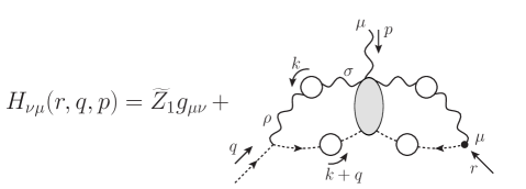
Figure 11.1: SDE for the ghost-gluon kernel, $H_{\nu\mu}(p,q,r)$, in compact form.

If we now combine Eqs. (7.1) and (7.18), it is clear that

$${P}_{\mu^{\prime}}^{\mu}(r){P}_{\nu^{\prime}}^{\nu}(p)\left[q^{\alpha}{\rm{I}}\!\Gamma_{\alpha\mu\nu}(q,r,p)\right]={P}_{\mu^{\prime}}^{\mu}(r){P}_{\nu^{\prime}}^{\nu}(p)[q^{\alpha}\Gamma_{\alpha\mu\nu}(q,r,p)+C_{\mu\nu}(q,r,p)]\,,$$ (11.4)

while from the STI of Eq. (2.33) we get

$${P}_{\mu^{\prime}}^{\mu}(r){P}_{\nu^{\prime}}^{\nu}(p)\left[q^{\alpha}{\rm{I}}\!\Gamma_{\alpha\mu\nu}(q,r,p)\right]={P}_{\mu^{\prime}}^{\mu}(r){P}_{\nu^{\prime}}^{\nu}(p)\,F(q^{2})\,{R}_{\nu\mu}(p,q,r)\,,$$ (11.5)

where

$${R}_{\nu\mu}(p,q,r):=\Delta^{-1}(p^{2})H_{\nu\mu}(p,q,r)-\Delta^{-1}(r^{2})H_{\mu\nu}(r,q,p)\,.$$ (11.6)

Then, equating the right-hand sides of Eqs. (11.4) and (11.5) we find

$$q^{\alpha}\left[{P}_{\mu^{\prime}}^{\mu}(r){P}_{\nu^{\prime}}^{\nu}(p)\Gamma_{\alpha\mu\nu}(q,r,p)\right]={P}_{\mu^{\prime}}^{\mu}(r){P}_{\nu^{\prime}}^{\nu}(p)\left[\,F(q^{2})\,{R}_{\nu\mu}(p,q,r)-C_{\mu\nu}(q,r,p)\right]\,.$$ (11.7)

The next step is to carry out the Taylor expansion of both sides of Eq. (11.7) around $q=0$, keeping terms that are at most linear in the momentum $q$.

The computation of the l.h.s. of Eq. (11.7) is straightforward, yielding

$$[{\rm l.h.s}]=q^{\alpha}{\cal T}_{\mu^{\prime}\nu^{\prime}}^{\mu\nu}(r)\Gamma_{\alpha\mu\nu}(0,r,-r)\,,\qquad{\cal T}_{\mu^{\prime}\nu^{\prime}}^{\mu\nu}(r):={P}_{\mu^{\prime}}^{\mu}(r){P}_{\nu^{\prime}}^{\nu}(-r)\,.$$ (11.8)

Given that $\Gamma_{\alpha\mu\nu}(0,r,-r)$ depends on a single momentum ($r$), its general tensorial decomposition is given by

$$\Gamma_{\alpha\mu\nu}(0,r,-r)=2{\cal A}_{1}(r^{2})\,r_{\alpha}g_{\mu\nu}+{\cal A}_{2}(r^{2})(r_{\mu}g_{\nu\alpha}+r_{\nu}g_{\mu\alpha})+{\cal A}_{3}(r^{2})\,r_{\alpha}r_{\mu}r_{\nu}\,.$$ (11.9)

Note that the form factors ${\cal A}_{i}(r^{2})$ do not contain poles; however, in general they are not regular functions. In particular, ${\cal A}_{1}(r^{2})$ diverges logarithmically as $r\to 0$, due to the “unprotected” logarithms that originate from the massless ghost loops appearing in the diagrammatic expansion of the vertex [253, 188]. These mild divergences do not interfere in any way with the arguments that follow.

It is now elementary to derive from Eq. (11.9) that

$${\cal T}_{\mu^{\prime}\nu^{\prime}}^{\mu\nu}(r)\Gamma_{\alpha\mu\nu}(0,r,-r)={\cal A}_{1}(r^{2})\lambda_{\mu^{\prime}\nu^{\prime}\alpha}(r)\,,\qquad\lambda_{\mu\nu\alpha}(r):=2r_{\alpha}P_{\mu\nu}(r)\,,$$ (11.10)

and, consequently, Eq. (11.8) becomes

$$[{\rm l.h.s}]={\cal A}_{1}(r^{2})\,q^{\alpha}\lambda_{\mu^{\prime}\nu^{\prime}\alpha}(r)\,.$$ (11.11)

The computation of the r.h.s. of Eq. (11.7) is considerably more technical; the main steps involved may be summarized as follows [146].

(i) The action of the projectors ${P}_{\mu^{\prime}}^{\mu}(r){P}_{\nu^{\prime}}^{\nu}(p)$ on $C_{\mu\nu}(q,r,p)$ activates Eq. (7.18); consequently, only the term $V_{1}(q,r,p)g_{\mu\nu}$ contributes to lowest order in $q$.

(ii) From Eq. (11.6) follows immediately that ${R}_{\nu\mu}(-r,0,r)=0$; thus, the vanishing of the zeroth order contribution in Eq. (11.7) imposes the condition

$$V_{1}(0,r,-r)=0\,,$$ (11.12)

in exact analogy to Eq. (9.8). Quite interestingly, we have arrived once again at the result of Eq. (7.19), but through a completely different set of arguments; indeed, while Eq. (7.19) is enforced by the Bose symmetry of the three-gluon vertex, Eq. (11.12) is a direct consequence of the STI satisfied by this vertex.

(iii) Clearly, the Taylor expansion of Eq. (11.7) involves the differentiation of the ghost-gluon kernel, which proceeds by invoking Eq. (11.1); specifically, to lowest order in $q$, we encounter the partial derivatives

$$\left[\frac{\partial H_{\nu\mu}(p,q,r)}{\partial q^{\alpha}}\right]_{q=0}\!\!\!\!\!\!=K_{\nu\mu\alpha}(-r,0,r)\,,\qquad\left[\frac{\partial H_{\mu\nu}(r,q,p)}{\partial q^{\alpha}}\right]_{q=0}\!\!\!\!\!\!=K_{\mu\nu\alpha}(r,0,-r)\,.$$ (11.13)

Employing the tensorial decomposition [182],

$$K_{\mu\nu\alpha}(r,0,-r)=-\frac{{\cal W}(r^{2})}{r^{2}}g_{\mu\nu}r_{\alpha}+\cdots\,,$$ (11.14)

where the ellipsis denotes terms that get annihilated upon contraction with the projector ${\cal T}_{\mu^{\prime}\nu^{\prime}}^{\mu\nu}(r)$. Then, combining Eq. (11.14) with the elementary relation ${\cal T}_{\mu^{\prime}\nu^{\prime}}^{\mu\nu}(r)K_{\nu\mu\alpha}(-r,0,r)=-{\cal T}_{\mu^{\prime}\nu^{\prime}}^{\mu\nu}(r)K_{\mu\nu\alpha}(r,0,-r)$, we may finally express the partial derivatives of Eq. (11.13) in terms of the function ${\cal W}(r^{2})$.

Taking the above three items into account, it is straightforward to show that the r.h.s. of Eq. (11.7) assumes the form

$$[{\rm r.h.s}]=q^{\alpha}\lambda_{\mu^{\prime}\nu^{\prime}\alpha}(r)\left[F(0)\left\{\widetilde{Z}_{1}\frac{d\Delta^{-1}(r^{2})}{dr^{2}}+\frac{{\cal W}(r^{2})}{r^{2}}\Delta^{-1}(r^{2})\right\}-{\mathbb{C}}(r^{2})\right]\,.$$ (11.15)

The final step is to equate the terms linear in $q$ that appear in Eqs. (11.11) and (11.15), and thus to obtain the WI

$${\cal A}_{1}(r^{2})=F(0)\left\{\widetilde{Z}_{1}\frac{d\Delta^{-1}(r^{2})}{dr^{2}}+\frac{{\cal W}(r^{2})}{r^{2}}\Delta^{-1}(r^{2})\right\}-{\mathbb{C}}(r^{2})\,.$$ (11.16)

Thus, the inclusion of the term $V_{\alpha\mu\nu}(q,r,p)$ in the three-gluon vertex leads ultimately to the displacement of the WI satisfied by the vertex form factor ${\cal A}_{1}(r^{2})$ by an amount given by the function ${\mathbb{C}}(r^{2})$.

12 The displacement function from lattice inputs

As stressed right after Eq. (9.18), the functional form of ${\mathbb{C}}(r^{2})$ may be determined from the “mismatch” between quantities entering in the WI of a given vertex. In this section we turn to what may be described as an independent confirmation of the Schwinger mechanism in QCD: a non-vanishing ${\mathbb{C}}(r^{2})$ is uncovered from the Euclidean version of Eq. (11.16), using inputs obtained almost exclusively from lattice simulations [148]. The crucial conceptual advantage of such a determination is that the lattice is intrinsically “blind” to field theoretic constructs such as the Schwinger mechanism; indeed, the lattice Green functions are generated by means of the model-independent functional averaging over gauge-field configurations. In that sense, the emergence of a nontrivial signal for ${\mathbb{C}}(r^{2})$ strongly supports the notion that the Schwinger mechanism is indeed operational in the gauge sector of QCD.

In order to employ profitably Eq. (11.16), we must establish an instrumental relation between the form factor ${\cal A}_{1}(r^{2})$ and a special projection of the three-gluon vertex, which has been studied extensively in various lattice simulations [262, 257, 263, 264, 265, 244, 266, 247, 267, 233, 22, 190, 252]. In particular, the lattice quantity we consider is the denominated “soft-gluon” form factor, denoted by $\mathit{L}_{{sg}}(r^{2})$, which corresponds to a particular case of Eq. (7.11): we set $\lambda_{\alpha\mu\nu}(q,r,p)\to\Gamma_{\!0\,\alpha\mu\nu}(q,r,p)$, and then take the limit $q\to 0$, i.e.,

$$\mathit{L}_{{sg}}(r^{2}) = \frac{\Gamma_{\!0\,\alpha\mu\nu}(q,r,p)P^{\alpha\alpha^{\prime}}(q)P^{\mu\mu^{\prime}}(r)P^{\nu\nu^{\prime}}(p){\rm{I}}\!\Gamma_{\alpha^{\prime}\mu^{\prime}\nu^{\prime}}(q,r,p)}{\rule[0.0pt]{0.0pt}{12.80365pt}\;{\Gamma_{\!0\,\alpha\mu\nu}(q,r,p)P^{\alpha\alpha^{\prime}}(q)P^{\mu\mu^{\prime}}(r)P^{\nu\nu^{\prime}}(p)\Gamma_{\!0\,\alpha^{\prime}\mu^{\prime}\nu^{\prime}}(q,r,p)}}\rule[0.0pt]{0.0pt}{14.22636pt}\Bigg{|}_{\begin{subarray}{c}\!\!q\to 0\\ p\to-r\end{subarray}}\,.$$ (12.1)

Evidently, when the decomposition of ${\rm{I}}\!\Gamma_{\alpha^{\prime}\mu^{\prime}\nu^{\prime}}(q,r,p)$ given by Eq. (7.1) is substituted into Eq. (12.1), the term $V_{\alpha^{\prime}\mu^{\prime}\nu^{\prime}}(q,r,p)$ drops out from Eq. (12.1) due to the validity of Eq. (7.4), producing the effective replacement ${\rm{I}}\!\Gamma_{\alpha^{\prime}\mu^{\prime}\nu^{\prime}}(q,r,p)\to\Gamma_{\alpha^{\prime}\mu^{\prime}\nu^{\prime}}(q,r,p)$.

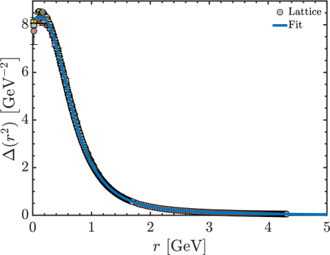
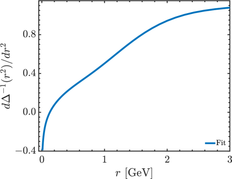
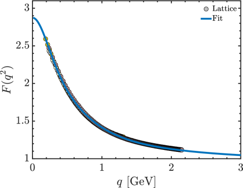
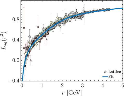
Figure 12.1: Upper panel: The gluon propagator (left) and the first derivative of its inverse (right). Lower panel: The ghost dressing function (left) and the soft gluon form factor $\mathit{L}_{{sg}}(r^{2})$ of the three-gluon vertex (right). All items are taken from [23], and have been cured from volume and discretization artifacts. Note that $\mathit{L}_{{sg}}(r^{2})$ is markedly below unity in the infrared, displaying the characteristic zero crossing and the attendant logarithmic divergence at the origin [253, 188, 189, 268, 199, 269, 252].

Then, the numerator, ${\cal N}$, and denominator, ${\cal D}$, of the fraction on the r.h.s. of Eq. (12.1), after employing Eq. (11.9), become

$${\cal N}=4(d-1)[r^{2}-(r\cdot q)^{2}/q^{2}]{\cal A}_{1}(r^{2})\,,\qquad{\cal D}=4(d-1)[r^{2}-(r\cdot q)^{2}/q^{2}]\,.$$ (12.2)

Crucially, when the ratio ${\cal N}/{\cal D}$ is formed, the path-dependent contribution contained in the square bracket cancels out, and Eq. (12.1) yields the final relation [23]

$$\mathit{L}_{{sg}}(r^{2})={\cal A}_{1}(r^{2})\,.$$ (12.3)

Thus, we reach the important conclusion that the form factor ${\cal A}_{1}(r^{2})$ appearing in Eq. (11.16) is precisely the one measured on the lattice in the soft-gluon kinematics. Therefore, Eq. (12.3) will be employed in Eq. (11.16), in order to substitute ${\cal A}_{1}(r^{2})$ in favor of $\mathit{L}_{{sg}}(r^{2})$.

Next, we convert Eq. (11.16) from Minkowski to Euclidean space, using the transformation rules given in Eqs. (A.2), (A.3), and (A.4), and solve for ${\mathbb{C}}(r^{2})$ to obtain (suppressing the indices “${\rm E}$”)

$${\mathbb{C}}(r^{2})=\mathit{L}_{{sg}}(r^{2})-L_{0}(r^{2})\,.$$ (12.4)

where

$$L_{0}(r^{2})=F(0)\left\{\frac{{\cal W}(r^{2})}{r^{2}}\Delta^{-1}(r^{2})+\widetilde{Z}_{1}\frac{d\Delta^{-1}(r^{2})}{dr^{2}}\right\}\,.$$ (12.5)

The quantity $L_{0}(r^{2})$ introduced above is precisely the value that $\mathit{L}_{{sg}}(r^{2})$ would have in the absence of the Schwinger mechanism, i.e., if ${\mathbb{C}}(r^{2})$ were to vanish identically.

As mentioned at the beginning of this section, the idea now is to use lattice inputs for the quantities appearing on the r.h.s. of Eq. (12.4). In doing so, we note that $L_{0}(r^{2})$ in Eq. (12.5) may not be reconstructed in its entirety from lattice ingredients, because the function ${\cal W}(r^{2})$ has not been simulated on the lattice. In particular, we will choose the inputs in the following way.

(${\it i}$) For the gluon propagator $\Delta(r^{2})$ we use the lattice data of [23], shown on the upper left panel of Fig. 12.1; the functional form of the fit (blue curve) is given in Eq. (C11) of [146].

(${\it ii}$) The derivative of the inverse propagator is obtained by differentiating the fit of $\Delta(r^{2})$ from the previous step, obtaining the curve shown on the upper right panel of Fig. 12.1.

(${\it iii}$) The $F(0)$ is obtained from the lattice results of [146] for the ghost dressing function. Even though only the value of this curve at the origin, namely $F(0)=2.88$ is required for the computation in hand, for future reference we show the entire curve $F(r^{2})$ on the lower left panel of Fig. 12.1.

(${\it iv}$) For the soft-gluon form factor $\mathit{L}_{{sg}}(r^{2})$ we use the lattice results of [190], shown on the lower right panel of Fig. 12.1. In particular, we employ the fit [blue curve] given by Eq. (C12) in [146].

(${\it v}$) All lattice curves shown in Fig. 12.1 are renormalized within the asymmetric MOM scheme, see App. B. In all cases the renormalization point has been chosen to be $\mu=4.3$ MeV.

(${\it vi}$) The finite value of the ghost-gluon renormalization constant, ${\widetilde{Z}}_{1}$, is determined nonperturbatively from the coupled system of SDEs governing the ghost propagator and ghost-gluon vertex, where ${\widetilde{Z}}_{1}$ appears explicitly. Specifically, this system is solved with lattice inputs renormalized in the asymmetric MOM scheme, for various values of ${\widetilde{Z}}_{1}$ until the $\chi^{2}$ deviation between the solution for $F(q^{2})$ and the lattice data of [23] is minimized. The procedure is detailed in Sec. 8 of [99] and yields ${\widetilde{Z}}_{1}=0.9333\pm 0.0075$.

(${\it vii}$) The function ${\cal W}(r^{2})$ is determined from the SDE obeyed by the ghost-gluon kernel. The computation, which is rather technical, is described in App. F; the resulting curve for ${\cal W}(r^{2})$ is shown as blue continuous on the left panel of Fig. 22.2.

The inputs (${\it i}$), (${\it ii}$), (${\it iii}$), (${\it vi}$), and (${\it vii}$) allow us to compute $L_{0}(r^{2})$, which is to be compared to the $\mathit{L}_{{sg}}(r^{2})$ of item (${\it iv}$); the comparison is shown on the left panel of Eq. (12.2). Then, using directly Eq. (12.4), a nontrivial result emerges for ${\mathbb{C}}(r^{2})$, represented by the black curve on the right panel of Fig. 12.2. The green error band surrounding this curve represents the total propagation of the individual errors assigned to the inputs employed in Eq. (12.4). Note that the resulting curve is negative throughout the entire range of available momenta, in agreement with the observation in item (${\it i}$) below Eq. (8.16).

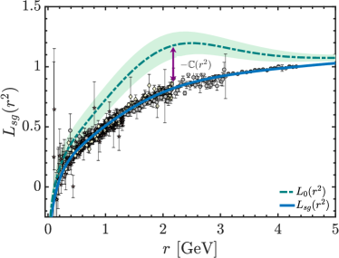
Figure 12.2: Left: Lattice data of [190] for $\mathit{L}_{{sg}}(r^{2})$ (points), the corresponding fit (blue continuous), and the null hypothesis prediction, $L_{0}(r^{2})$, of Eq. (12.4) (green dot-dashed). Right: Result for ${\mathbb{C}}(r^{2})$ (black continuous line) obtained from Eq. (12.4); the error error bars correspond to the combined error propagated from $\mathit{L}_{{sg}}$ and ${\cal W}$. The green band is obtained by implementing separate $\chi^{2}$ fits to the upper and lower bounds of the points; its purpose is to provide a visual impression of the typical error associated with ${\mathbb{C}}(r^{2})$.

The clear departure of the black curve from the line ${\mathbb{C}}=0$, indicates that the null hypothesis (absence of Schwinger mechanism) is strongly disfavored. In fact, as was explained in [148], even if the errors in all data points for ${\mathbb{C}}(r^{2})$ were $95\%$ larger, i.e., nearly doubled, we could still discard the null hypothesis at the $5\sigma$ confidence level.

13 STI consistency and need for double Schwinger poles

It is clear from the discussion of the previous sections that the saturation of the gluon propagator at the origin requires the vertices of the theory to contain massless poles. Quite interestingly, as was demonstrated in [149], the reverse is also true: if the gluon propagator saturates at the origin, the STI of Eq. (2.33) forces the three-gluon vertex to contain precisely this kind of poles.

To begin our analysis, we decompose the ghost-gluon kernel, $H_{\mu\nu}(r,q,p)$, appearing in Eq. (2.33), into its most general Lorentz structure, namely [215]

$$H_{\mu\nu}(r,q,p)=g_{\nu\mu}A_{1}+r_{\mu}r_{\nu}A_{2}+p_{\mu}p_{\nu}A_{3}+p_{\mu}r_{\nu}A_{4}+r_{\mu}p_{\nu}A_{5}\,,$$ (13.1)

where $A_{i}\equiv A_{i}(r,q,p)$. At tree level, $A_{1}^{(0)}=1$, while all other form factors vanish. Since the $H_{\mu\nu}(r,q,p)$ in Eq. (2.33) appears contracted by transverse projectors, only the form factors $A_{1}$, $A_{3}$, and $A_{4}$ contribute to the STI.

Note that while $H_{\mu\nu}(r,p,q)$ may itself contain poles longitudinally coupled to its gluon leg, their residues are known to be negligible in comparison to those of the three-gluon vertex [144, 146, 149]. Hence, for simplicity, we will assume here that $H_{\mu\nu}(r,p,q)$ is pole-free. For the complete analysis, where the poles of the ghost-gluon kernel are taken into account, see [149].

Next, we decompose both sides of Eq. (2.33) in the same basis, and equate the coefficients of the independent tensor structures. Note that each side of the STI has two free Lorentz indices, and two independent momenta; hence, they can be decomposed in the same basis used for $H_{\mu\nu}(r,p,q)$ in Eq. (13.1). In particular, for the contraction of the gluon momentum with the pole-free part of the vertex, we write

$$q^{\alpha}\Gamma_{\alpha\mu\nu}(q,r,p)=S_{1}g_{\mu\nu}+S_{2}r_{\mu}r_{\nu}+S_{3}p_{\mu}p_{\nu}+S_{4}p_{\mu}r_{\nu}+S_{5}r_{\mu}p_{\nu}\,,$$ (13.2)

with $S_{i}\equiv S_{i}(q,r,p)$. At tree level, $S_{1}^{(0)}=p^{2}-r^{2}$, $S_{2}^{(0)}=1$, $S_{3}^{(0)}=-1$, and $S_{4}^{(0)}=S_{5}^{(0)}=0$. From Bose symmetry, $S_{1}$, $S_{4}$ and $S_{5}$ must be anti-symmetric under the exchange of $r\leftrightarrow p$, such that

$$S_{1}(0,r,-r)=S_{4}(0,r,-r)=S_{5}(0,r,-r)=0\,.$$ (13.3)

Then, since $\Gamma_{\alpha\mu\nu}(q,r,p)$ is, by definition, pole-free, its contraction with $q^{\alpha}$ vanishes when $q=0$; thus, from Eqs. (13.2) and (13.3),

$$S_{2}(0,r,-r)=-S_{3}(0,r,-r)\,.$$ (13.4)

Consider then the pole part; contracting Eq. (7.12) with $q^{\alpha}$, we obtain

$$q^{\alpha}{\cal V}_{\alpha\mu\nu}(q,r,p)=V_{1}g_{\mu\nu}+\frac{{\overline{V}}\vphantom{V}_{2}}{r^{2}}r_{\mu}r_{\nu}+\frac{{\overline{V}}\vphantom{V}_{3}}{p^{2}}p_{\mu}p_{\nu}+V_{2}p_{\mu}r_{\nu}+\frac{{\overline{V}}\vphantom{V}_{5}}{r^{2}p^{2}}r_{\mu}p_{\nu}\,,$$ (13.5)

where the ${\overline{V}}\vphantom{V}_{i}\equiv{\overline{V}}\vphantom{V}_{i}(q,r,p)$ are given by

$${\overline{V}}\vphantom{V}_{2}= -V_{3}-(p\cdot q)V_{4}-2V_{7}\,,\qquad{\overline{V}}\vphantom{V}_{3}=-V_{5}-(r\cdot q)V_{6}+2V_{9}\,,$$

$${\overline{V}}\vphantom{V}_{5}= V_{10}+(p^{2}-r^{2})V_{8}-p^{2}\left[V_{3}+(q\cdot p)V_{4}+V_{7}\right]-r^{2}\left[V_{5}+(q\cdot r)V_{6}-V_{9}\right]\,.$$ (13.6)

With the above decompositions, we proceed to match the coefficients of the independent tensor structures on both sides of Eq. (2.33). We begin with the tensors $r_{\mu}r_{\nu}$ and $p_{\mu}p_{\nu}$, whose coefficients give, respectively,

$$S_{2}= \,\frac{1}{r^{2}}\left\{F(q^{2})\left\{\Delta^{-1}(r^{2})\left[A_{1}(r,q,p)+(p\cdot r)A_{4}(r,q,p)\right]+r^{2}\Delta^{-1}(p^{2})A_{3}(p,q,r)\right\}\!-\!{\overline{V}}\vphantom{V}_{2}\right\}\,,$$

$$S_{3}= \,-\frac{1}{p^{2}}\left\{F(q^{2})\left\{p^{2}\Delta^{-1}(r^{2})A_{3}(r,q,p)+\Delta^{-1}(p^{2})\left[A_{1}(p,q,r)+(p\cdot r)A_{4}(p,q,r)\right]\right\}+{\overline{V}}\vphantom{V}_{3}\right\}\,.$$ (13.7)

Now, consider the $S_{3}$ in Eq. (13.7), which is proportional to the factor $1/p^{2}$. Since, by definition, $S_{3}$ is pole-free, the expression in curly brackets must vanish when $p\to 0$, in order for the r.h.s. of Eq. (13.7) to be an evitable singularity. This condition then requires

$$V_{9}(q^{2})=\frac{1}{2}m^{2}F(q^{2})A_{1}(q^{2})\,,$$ (13.8)

where, in Minkowski space, $m^{2}=-\Delta^{-1}(0)$, and we define

$$V_{9}(q^{2}):=V_{9}(q,-q,0)\,,\qquad A_{1}(q^{2}):=A_{1}(0,q,-q)\,.$$ (13.9)

Evidently, $V_{9}(q^{2})$ is non-zero if the gluon propagator saturates at the origin. Hence, from Eq. (7.12) follows that ${\cal V}_{\alpha\mu\nu}(q,r,p)$ contains a pole at $p=0$ in the tensor structure $p_{\nu}q_{\alpha}$.

A relation similar to Eq. (13.9) can be obtained for the $q=0$ limit of $V_{9}(q,r,p)$. Specifically, it follows from the Bose symmetry of the pole vertex, i.e.,

$${\cal V}_{\alpha\mu\nu}(q,r,p)=-{\cal V}_{\mu\alpha\nu}(r,q,p)=-{\cal V}_{\nu\mu\alpha}(p,r,q)\,,$$ (13.10)

that the form factors $V_{i}(q,r,p)$ satisfy

$$V_{1,2}(q,r,p)= \,-V_{1,2}(q,p,r)\,,\quad V_{7}(q,r,p)= \,V_{7}(r,q,p)\,,$$

$$V_{3,4}(q,r,p)= \,-V_{3,4}(p,r,q)\,,\quad V_{8}(q,r,p)= \,V_{8}(q,p,r)\,,$$

$$V_{5,6}(q,r,p)= \,-V_{5,6}(r,q,p)\,,\quad V_{9}(q,r,p)= \,V_{9}(p,r,q)\,,$$ (13.11)

while $V_{10}(q,r,p)$ is totally anti-symmetric. Furthermore, Bose symmetry relates some form factors to each other by cyclic permutations of their arguments. Specifically,

$$V_{3,4}(q,r,p)= \,V_{1,2}(r,p,q)\,,\qquad V_{8}(q,r,p)= \,V_{7}(r,p,q)\,,$$

$$V_{5,6}(q,r,p)= \,V_{1,2}(p,q,r)\,,\qquad V_{9}(q,r,p)= \,V_{7}(p,q,r)\,.$$ (13.12)

Then, combining Eqs. (13.11) and (13.8), it follows that

$$V_{9}(0,q,-q)=V_{9}(q^{2})\,,$$ (13.13)

such that the tensor structure $p_{\nu}q_{\alpha}$ of ${\cal V}_{\alpha\mu\nu}(q,r,p)$ has a pole also at $q=0$.

Now, neither $F(0)$ nor $A_{1}(0)$ vanish in Landau gauge. In particular, as was demonstrated in [182], in this gauge,

$$A_{1}(0)={\widetilde{Z}}_{1}\,,$$ (13.14)

where we recall that the ghost-gluon renormalization constant, ${\widetilde{Z}}_{1}$, is finite by virtue of Taylor’s theorem [102]. Hence, in the limit when both $q$ and $p$ vanish, $V_{9}(q,r,p)/q^{2}p^{2}$ behaves as a double pole,

$$\lim_{q\to 0}\lim_{p\to 0}\frac{V_{9}(q,r,p)}{q^{2}p^{2}}=\lim_{q\to 0}\lim_{p\to 0}\frac{{\widetilde{Z}}_{1}F(0)m^{2}}{2q^{2}p^{2}}\,.$$ (13.15)

Similarly, requiring that the $S_{2}$ of Eq. (13.7) must be pole-free at $r=0$, we obtain an expression identical to Eq. (13.8), but with $V_{9}(q^{2})$ substituted by $V_{7}(q,0,-q)$. Thus, ${\cal V}_{\alpha\mu\nu}(q,r,p)$ contains a pole at $r=0$ in the structure $q_{\alpha}r_{\mu}$. Indeed, the same conclusion follows from Eq. (13.8) and the Bose symmetry relations of Eqs. (13.11) and (13.12). In fact, combining Eqs. (13.11) and (13.12) we get

$$V_{7}(0,q,-q)=V_{7}(0,q,-q)=V_{8}(q,-q,0)=V_{8}(q,0,-q)=V_{9}(q^{2})\,.$$ (13.16)

Hence, all of the mixed double poles of ${\cal V}_{\alpha\mu\nu}$ in Eq. (7.12) are characterized by the same function $V_{9}(q^{2})$. To appreciate its nature, consider as an analogy a general function of two variables, $x$ and $y$, of the form $f(x,y)=g(x,y)/xy$, and assume $g(x,0)\neq 0$ and $g(0,y)\neq 0$. Then, $f(x,y)$ has simple poles as $x\to 0$ and $y\to 0$. In particular, for $y\to 0$, the residue of the associated pole is a function of $x$, given by $r(x)=g(x,0)/x$. The latter has itself a pole at $x=0$, with residue $g(0,0)\neq 0$. Evidently, $g(x,0)$ plays the role of $V_{9}(q^{2})$.

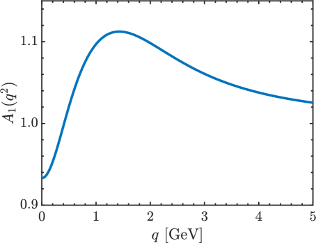
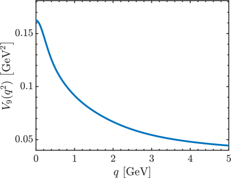
Figure 13.1: Left: Form factor $A_{1}(q^{2})$ of the ghost-gluon scattering kernel in the soft-antighost limit, determined in [215], and converted to the asymmetric MOM scheme through rescaling by a factor of $0.933$ [148]. Right: The function $V_{9}(q^{2})$, associated with the mixed double poles of the three-gluon vertex, determined through Eq. (13.8).

At this point, the function $V_{9}(q^{2})$ can be determined numerically from Eq. (13.8), using the known forms of the gluon and ghost propagators, and the ghost-gluon form factor, $A_{1}(q^{2})$.

Evidently, since $V_{9}(q^{2})$ is a component of the three-gluon vertex, it depends on the renormalization scheme and point chosen, and so do the $F(q^{2})$, $A_{1}(q^{2})$ and $m^{2}$ appearing in Eq. (13.8). Following the convention adopted throughout this work, we renormalize all ingredients in the asymmetric MOM scheme (see App. B), choosing $\mu=4.3$ GeV for the renormalization point. For $F(q^{2})$ we employ the fit to lattice data of [23], shown as a blue curve on the lower left panel of Fig. 12.1. Then, for $A_{1}(q^{2})$ we use the SDE result of [215], originally renormalized in the so-called “Taylor scheme” [102, 258, 270, 271, 23], after rescaling by a factor of $0.933$ [148] to convert it to the asymmetric MOM scheme; the converted form is shown on the left panel of Fig. 13.1. Finally, we use the value $m=354$ MeV, deduced from the lattice determination of the gluon propagator in [23]. The resulting $V_{9}(q^{2})$ is shown on the right panel of Fig. 13.1; note that it tends to zero at large momentum. Comparing the result for $V_{9}(q^{2})$ in Fig. 13.1 to the fit for $F(q^{2})$ in Fig. 12.1, it is clear that the shape of $V_{9}(q^{2})$ is dominated by $F(q^{2})$, whereas $A_{1}(q^{2})$ contributes modestly, supplying a $12\%$ enhancement at momenta $q\sim 1.5$ GeV.

It is similarly possible to derive constraints on the remaining form factors $V_{i}$, by analyzing the tensor structures $g_{\mu\nu}$, $r_{\nu}p_{\mu}$ and $r_{\mu}p_{\nu}$ of Eq. (2.33). Specifically, one can show

(i) The STI constraints derived for $i=1,3,5$ are equivalent to the WI displacement presented in Sec. 11.

(ii) In the case $i=2,4,6$, the Bose symmetry relations of Eq. (13.11) imply

$$V_{2}(0,r,-r)=V_{4}(q,0,-q)=V_{6}(q,-q,0)=0\,,$$ (13.17)

in analogy to Eq. (7.19). Then, the $r_{\nu}p_{\mu}$ component of Eq. (2.33) leads to certain constraints on the derivatives of the corresponding $V_{i}$, which we do not report here.

(iii) Finally, given that in Eq. (7.12) the $V_{10}(q,r,p)$ is accompanied by a denominator $q^{2}r^{2}p^{2}$, one might expect that this combined term should act as a triple mixed pole. However, as was shown in [149], this is not the case. Instead, equating the $r_{\mu}p_{\nu}$ component of the STI of Eq. (2.33), one may show that $V_{10}$ vanishes rapidly at small momenta, thus reducing substantially the order of the pole associated with this form factor [149].

14 Bound state realization of the Schwinger mechanism

In the previous sections we have elucidated how the presence of massless poles in the three-gluon and ghost-gluon vertices induces a mass scale at the level of the gluon propagator. Our arguments have been predominantly based on symmetries, and, in particular, the special way in which the STI of Eq. (2.33) is resolved in terms of these poles. However, two fundamental questions remain to be addressed. First, the identification of the precise dynamical mechanism that gives rise to the formation of the Schwinger poles. Second, the determination of ${\mathbb{C}}(r^{2})$ not through the indirect lattice derivation presented in Sec. 12, but rather directly, from the equation that governs its evolution. In fact, as we will show in detail, the structure of this equation leads to a striking simplification, allowing us to carry out the multiplicative renormalization of the mass formula given in Eq. (8.16) exactly.

The dynamical picture that will be outlined in the next sections may be summarized as follows. The Schwinger poles in the vertices are produced dynamically, when elementary Yang-Mills fields (e.g., two gluons, two ghosts, or three gluons) merge to form composite colored scalars with vanishing masses [272, 273, 92, 142, 93, 203, 81], to be denoted by $\Phi^{a}$. These nonperturbative processes are controlled by special bound state equations, analogous to the standard BSEs [96, 143, 97, 55, 144, 147, 146, 100]; and the corresponding BS amplitudes are (up to finite multiplicative constants) the residue functions.

From now on we simplify the discussion, focusing exclusively on the three gluon vertex, which captures the bulk of the full effect [144]. In this case, the Schwinger poles arise through the fusion of a pair of gluons; there are three main structures associated with this special process, which are diagrammatically depicted in Fig. 14.1:

(a) The effective vertex describing the interaction between $\Phi^{a}$ and two gluons, denoted by

$$B^{abc}_{\mu\nu}(q,r,p)=if^{abc}B_{\mu\nu}(q,r,p)\,.$$ (14.1)

(b) The propagator of the massless composite scalar, having the form

$$D^{ab}_{\Phi}(q)=\frac{i\delta^{ab}}{q^{2}}\,.$$ (14.2)

(c) The transition amplitude, $I^{ab}_{\alpha}(q)=\delta^{ab}I_{\alpha}(q)$, connecting a gluon $A^{a}_{\alpha}$ with a scalar $\Phi^{b}$. Evidently, Lorentz invariance imposes that

$$I_{\alpha}(q)=q_{\alpha}I(q^{2})\,,$$ (14.3)

where $I(q^{2})$ is a scalar form factor.

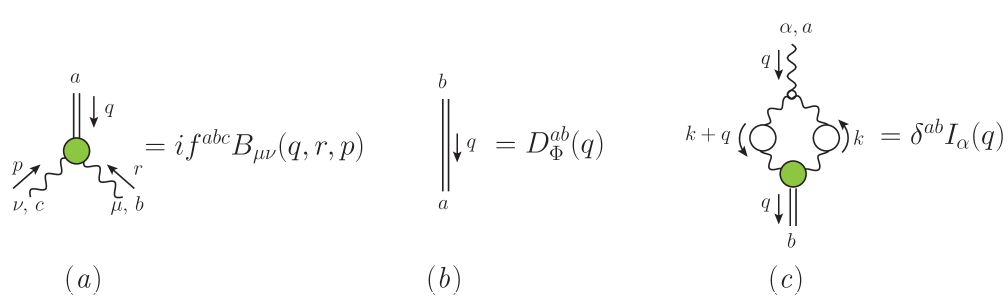
Figure 14.1: Left: The effective vertex $B^{abc}_{\mu\nu}(q,r,p)$, with Lorentz, color, and momentum conventions indicated. Center: The propagator of the massless composite scalar, $D_{\Phi}^{ab}(q)$. Right: Gluon-scalar transition amplitude, $I^{ab}_{\alpha}(q)$.

The emergence of these three items, (a)-(c), modifies crucially the structure of the four-gluon kernel, ${\cal T}^{mnbc}_{\rho\sigma\mu\nu}(p_{1},p_{2},p_{3},p_{4})$, which enters in the skeleton expansion of the three-gluon vertex SDE. In particular, as shown diagrammatically in Fig. 14.2, we have that

$${\cal T}^{mnbc}_{\rho\sigma\mu\nu}(p_{1},p_{2},p_{3},p_{4})={\mathcal{K}}^{mnbc}_{\rho\sigma\mu\nu}(p_{1},p_{2},p_{3},p_{4})+{\mathcal{M}}^{mnbc}_{\rho\sigma\mu\nu}(p_{1},p_{2},p_{3},p_{4})\,,$$ (14.4)

where ${\mathcal{K}}$ denotes the standard pole-free term, while ${\mathcal{M}}^{mnbc}$ is given by

$${\mathcal{M}}^{mnbc}_{\rho\sigma\mu\nu}(p_{1},p_{2},p_{3},p_{4})=B^{mnx}_{\rho\sigma}(p_{1},p_{2},q)D^{xe}_{\Phi}(q)B^{ebc}_{\mu\nu}(p_{3},p_{4},-q)\,,$$ (14.5)

with $q=p_{1}+p_{2}=-p_{3}-p_{4}$.

We stress at this point that, despite appearances, the kernel ${\cal T}$ is one-particle irreducible, because the propagator $D_{\Phi}(q)$ in ${\mathcal{M}}$ does not represent a fundamental field of the Yang-Mills Lagrangian, but rather a composite excitation, the collective result of countless multi-gluonic interactions.

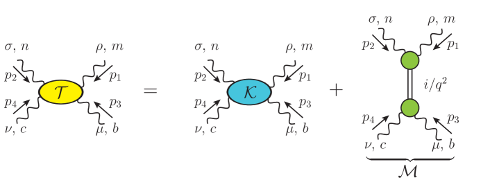
Figure 14.2: Decomposition of the four-gluon scattering kernel, ${\cal T}^{mnbc}_{\rho\sigma\mu\nu}(p_{1},p_{2},p_{3},p_{4})$, into a regular part, ${\cal K}^{mnbc}_{\rho\sigma\mu\nu}(p_{1},p_{2},p_{3},p_{4})$, and a massless pole part, ${\cal M}^{mnbc}_{\rho\sigma\mu\nu}(p_{1},p_{2},p_{3},p_{4})$, according to Eq. (14.4).

The massless pole in ${\mathcal{M}}$ is eventually transferred to the gluon self-energy through the full three-gluon vertex that appears in diagram ($a_{1}$) of Fig. 3.2. Specifically, consider the SDE for the three-gluon vertex, written from the point of view of the gluon leg carrying momentum $q$; this choice is dictated by the fact that $q$ has been identified with the momentum carried by the gluon propagator [see Fig. 3.2], while the other two channels are connected to propagators internal to the graph (carrying the integration momentum $k$). The diagrammatic representation of the vertex SDE is given in Fig. 14.3, where we only keep the diagrams relevant to our purposes (first row), while the omitted ones have no bearing on any of our conclusions [see comments following Eq. (14.8)].

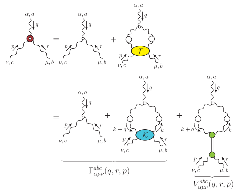
Figure 14.3: First line: SDE for the three-gluon vertex. Second line: The pole induced to the three-gluon vertex due to the component ${\cal M}$ of ${\cal T}$ in Eq. (14.4) (see also Fig. 14.2).

The inclusion of the term ${\mathcal{M}}^{mnbc}$ into the vertex SDE gives rise to a pole term, $V_{\alpha\mu\nu}$, for the three-gluon vertex (second row). In fact, the term that this procedure generates is precisely the $V_{\alpha\mu\nu}(q,r,p)$ introduced in Eq. (7.13).

Specifically, as may be read off from Fig. 14.3,

$$V_{\alpha\mu\nu}(q,r,p)=I_{\alpha}(q)\left(\frac{i}{q^{2}}\right)iB_{\mu\nu}(q,r,p)\,.$$ (14.6)

Then, by virtue of Eq. (14.3), this term becomes

$$V_{\alpha\mu\nu}(q,r,p)=-\left(\frac{q_{\alpha}}{q^{2}}\right)I(q^{2})B_{\mu\nu}(q,r,p)\,.$$ (14.7)

Since $V_{\alpha\mu\nu}(q,r,p)$ satisfies $P^{\alpha^{\prime}\alpha}(q)V_{\alpha\mu\nu}(q,r,p)=0$, we conclude that the bound-state realization of the Schwinger poles enforces their longitudinal nature dynamically.

The central result of this construction is obtained when the component $V_{\alpha\mu\nu}(q,r,p)$ of the three-gluon vertex ${\rm{I}}\!\Gamma_{\alpha\mu\nu}(q,r,p)$ is inserted into the SDE that determines the momentum evolution of the gluon propagator [see Fig. 3.2]: $V_{\alpha\mu\nu}(q,r,p)$ provides the massless pole required for the activation of the Schwinger mechanism.

To see this precisely, let us focus on the part of the gluon propagator proportional to $q_{\mu}q_{\nu}$. Then, we obtain immediately the characteristic diagram shown in Fig. 14.4, composed by the “square” of the transition amplitude $I_{\alpha}(q)$. When the limit $q\to 0$ is taken, one arrives at the fundamental result [92, 96, 97]

$$m^{2}=g^{2}I^{2}\,,$$ (14.8)

where the short-hand notation $I:=I(0)$ has been introduced.

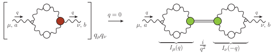
Figure 14.4: Relation between the gluon mass and the transition amplitude, $I_{\alpha}(q)$.

It is important to stress that in Figs. 14.3 and 14.4 all diagrams containing ghosts-gluon or four-gluon vertices have been omitted. The omission of these graphs has no impact on our qualitative conclusions for the following two reasons. First, as we will see in Sec. 20, the renormalization of Eq. (14.8) induces an extensive cancellation, which would eliminate all these graphs, provided that the ghost-gluon and four-gluon vertices contain no Schwinger poles. In omitting these terms we essentially assume that the pole residue of the four-gluon vertex is numerically subleading, as is known to happen in the case of the ghost-gluon vertex [144]. Second, the main function of the vertex SDE is to participate in the aforementioned cancellation, where the graph retained in Fig. 14.4 is precisely what one needs. In fact, while the quantity $\mathit{L}_{{sg}}(r^{2})$ is a key component in some of the fundamental formulas, its form will not be determined from the vertex SDE, but rather from extensive lattice simulations of the three-gluon vertex [188, 189, 247, 190, 23, 248, 249, 250, 251, 252].

The bound-state origin of the Schwinger poles may be used to explain the structure of not only the component $V_{\alpha\mu\nu}(q,r,p)$, but of the entire vertex ${\cal V}_{\alpha\mu\nu}(q,r,p)$, given Eq. (7.12). Indeed, as may be clearly seen in Fig. 14.5, in compliance with the Bose symmetry of ${\rm{I}}\!\Gamma_{\alpha\mu\nu}(q,r,p)$, Schwinger poles appear also in the channels carrying momenta $r$ or $p$, being proportional to $I_{\mu}(r)$ or $I_{\nu}(p)$. These structures, in turn, give rise to mixed poles, precisely as seen in Eq. (7.12). In fact, the effective amplitudes $B_{\mu\nu}$, $B_{\mu}$, and $B$ in Fig. 14.5 may be expressed in terms of the form factors $V_{i}$ in Eq. (7.12), through the direct matching of the various tensorial structures, namely

$$I(q^{2})B_{\mu\nu}(q,r,p)= \,-\left[g_{\mu\nu}V_{1}(q,r,p)+p_{\mu}r_{\nu}V_{2}(q,r,p)\right]\,,$$

$$I(q^{2})I(r^{2})B_{\nu}(q,r,p)= \,-(r-q)_{\nu}V_{7}(q,r,p)\,,$$

$$I(q^{2})I(r^{2})I(p^{2})B(q,r,p)= \,\,iV_{10}(q,r,p)\,.$$ (14.9)

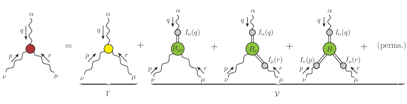
Figure 14.5: The general structure of the three-gluon vertex after the activation of the Schwinger mechanism. Note, in particular, that the term ${\cal V}_{\alpha\mu\nu}(q,r,p)$ contains single poles, such as $q_{\alpha}/q^{2}$, as well as mixed poles of the forms $q_{\alpha}r_{\mu}/q^{2}r^{2}$ and $q_{\alpha}r_{\mu}p_{\nu}/q^{2}r^{2}p^{2}$. The term “(perms)” denotes the permutations of the external legs that lead to a Bose-symmetric ${\cal V}_{\alpha\mu\nu}(q,r,p)$.

15 Some key limits

In this section we focus on the behavior of the two main building blocks, namely of the effective vertex $B_{\mu\nu}(q,r,p)$ and the transition amplitude $I(q^{2})$, as $q\to 0$.

The general tensorial decomposition of $B_{\mu\nu}(q,r,p)$ is given by

$$B_{\mu\nu}(q,r,p)=B_{1}\,g_{\mu\nu}+B_{2}\,r_{\mu}r_{\nu}+B_{3}\,p_{\mu}p_{\nu}+B_{4}\,r_{\mu}p_{\nu}+B_{5}\,p_{\mu}r_{\nu}\,,$$ (15.1)

where $B_{i}:=B_{i}(q,r,p)$ are scalar form factors.

The Bose symmetry of the full vertex $B^{abc}_{\mu\nu}(q,r,p)$ under the simultaneous exchange $(r,b,\mu)\leftrightarrow(p,c,\nu)$ means that $B^{abc}_{\mu\nu}(q,r,p)=B^{acb}_{\nu\mu}(q,p,r)$. Since $f^{abc}$ has been factored out in Eq. (14.1), we have that $B_{\mu\nu}(q,r,p)=-B_{\nu\mu}(q,p,r)$. Then, setting $q=0$   ($p=-r$) in this last relation, we find $B_{\mu\nu}(0,r,-r)=-B_{\nu\mu}(0,r,-r)$. So, since

$$B_{\mu\nu}(0,r,-r)=B_{1}(0,r,-r)\,g_{\mu\nu}+C_{1}(0,r,-r)r_{\mu}r_{\nu}\,,$$ (15.2)

where $C_{1}:=B_{2}+B_{3}-B_{4}-B_{5}$, we conclude that

$$B_{1}(0,r,-r)=0=C_{1}(0,r,-r)\,\,\,\Longrightarrow\,\,B_{\mu\nu}(0,r,-r)=0\,.$$ (15.3)

Let us proceed by considering the Taylor expansion of $B_{\mu\nu}(q,r,p)$ around $q=0$,

$$B_{\mu\nu}(0,r,-r)=q^{\alpha}{\cal B}_{\alpha\mu\nu}(0,r,-r)+\ldots\,,$$ (15.4)

where the ellipsis denotes terms of higher order in $q$, and the shorthand notation

$${\cal B}_{\alpha\mu\nu}(0,r,-r):=\left[\frac{\partial}{\partial q^{\alpha}}B^{\mu\nu}(q,r,\,-r-q)\right]_{q=0}\,,$$ (15.5)

has been introduced, supplemented by the diagrammatic representation shown in Fig. 15.1. Note that when taking the limit indicated in Eq. (15.5), the momentum $r$ is treated as independent of $q$; then, due to the conservation of four-momentum, $p$ depends on $q$, since $p=-q-r$, and therefore, $\partial p^{\mu}/\partial q^{\alpha}=-g^{\mu}_{\alpha}$.

We next consider the contraction of ${\cal B}_{\alpha\mu\nu}(0,r,-r)$ by $P_{\mu^{\prime}}^{\mu}(r)P_{\nu^{\prime}}^{\nu}(r)$; in the Landau gauge, this contraction occurs naturally in the diagrams where $B_{\mu\nu}(q,r,p)$ is inserted, because the two gluon propagators to which it is attached are completely transverse. Since the tensorial decomposition of ${\cal B}_{\alpha\mu\nu}(0,r,-r)$ is given by

$${\cal B}_{\alpha\mu\nu}(0,r,-r)={\cal B}_{1}(r^{2})\,r_{\alpha}g_{\mu\nu}+{\cal B}_{2}(r^{2})\left[r_{\mu}g_{\alpha\nu}+r_{\nu}g_{\mu\alpha}\right]+{\cal B}_{3}(r^{2})\,r_{\alpha}r_{\mu}r_{\nu}\,,$$ (15.6)

only the first term in Eq. (15.6) survives this contraction, namely

$${\cal B}_{\alpha\mu\nu}(0,r,-r)P_{\mu^{\prime}}^{\mu}(r)P_{\nu^{\prime}}^{\nu}(r)={\cal B}_{1}(r^{2})\,r_{\alpha}P_{\mu^{\prime}\nu^{\prime}}(r)\,.$$ (15.7)

It is then straightforward to establish that

$$r_{\alpha}{\cal B}_{1}(r^{2})=\left[\frac{\partial}{\partial q^{\alpha}}B_{1}(q,r,\,-r-q)\right]_{q=0}=2r_{\alpha}\underbrace{\left[\frac{\partial{B}_{1}(q,r,p)}{\partial p^{2}}\right]_{q=0}}_{\mathbb{B}(r^{2})}\,,$$ (15.8)

or

$${\cal B}_{1}(r^{2})=2\mathbb{B}(r^{2})\,,$$ (15.9)

from which follows that

$${\cal B}_{\alpha\mu\nu}(0,r,-r)=2\,\mathbb{B}(r^{2})\,r_{\alpha}g_{\mu\nu}+\ldots\,,$$ (15.10)

and then, from Eq. (15.4),

$$B_{\mu\nu}(0,r,-r)=2\,(q\cdot r)\,\mathbb{B}(r^{2})\,g_{\mu\nu}+\ldots\,,$$ (15.11)

where the ellipses denote terms that get annihilated upon the aforementioned contraction. The diagrammatic representation of Eq. (15.10) is shown in Fig. 15.1, and will be used in the analysis that follows.

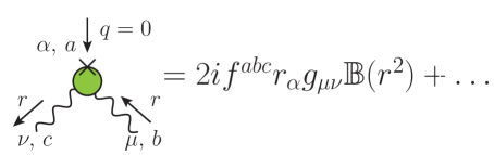
Figure 15.1: Diagrammatic representation of Eq. (15.10), corresponding to the first nonvanishing term in the Taylor expansion of $B_{\mu\nu}^{abc}(q,r,p)$ around $q=0$.

Finally, combining Eqs. (7.20), (14.6) and (15.11), we obtain a relation between the displacement function, ${\mathbb{C}}(r^{2})$, and the BS amplitude, $\mathbb{B}(r^{2})$, namely

$${\mathbb{C}}(r^{2}):=-I\,\mathbb{B}(r^{2})\,,$$ (15.12)

which is the result announced in item ($a$) of Sec 7.

We next turn to the transition amplitude ${I}^{\alpha}(q)$. In view of the central relation given by Eq. (14.8), we must determine the quantity $I$ in terms of the basic elements entering in its diagrammatic definition, shown on item (iii) of Fig. 14.1.

In particular, the transition amplitude ${I}^{\alpha}(q)$ for general momentum $q$ is given by

$$I^{\alpha}(q)=-\frac{iC_{\rm A}}{2}\int_{k}\Gamma_{\!0}^{\alpha\beta\lambda}(q,k,-t)\Delta_{\beta\mu}(k)\Delta_{\lambda\nu}(t)B^{\mu\nu}(-q,-k,t)\,,$$ (15.13)

where Eq. (14.1) was employed, $t:=k+q$, and the symmetry factor $\frac{1}{2}$ has been included.

Then, from Eq. (14.3), it is elementary to deduce that

$$I=\frac{1}{4}\left[\frac{\partial I^{\alpha}(q)}{\partial q^{\alpha}}\right]_{q=0}\,.$$ (15.14)

Thus, from Eq. (15.13) we obtain

$$4I= \,-\frac{iC_{\rm A}}{2}\int_{k}\left[\frac{\partial}{\partial q^{\alpha}}\Gamma_{\!0}^{\alpha\beta\lambda}(q,k,-t)\Delta_{\beta\mu}(k)\Delta_{\lambda\nu}(t)\right]_{q=0}\!\!\!\!\!\!B^{\mu\nu}(0,-k,k)$$

$$\,-\frac{iC_{\rm A}}{2}\int_{k}\Gamma_{\!0}^{\alpha\beta\lambda}(0,k,-k)\Delta_{\beta}^{\mu}(k)\Delta_{\lambda}^{\nu}(k)\,{\cal B}_{\alpha\mu\nu}(0,-k,k)\,,$$ (15.15)

and, since $B_{\mu\nu}(0,-k,k)=0$ [see Eq. (15.3)], we simply have

$$4I=-\frac{iC_{\rm A}}{2}\int_{k}\Gamma_{\!0}^{\alpha\beta\lambda}(0,k,-k)\Delta_{\beta}^{\mu}(k)\Delta_{\lambda}^{\nu}(k)\,{\cal B}_{\alpha\mu\nu}(0,-k,k)\,.$$ (15.16)

Eq. (15.16) may be further evaluated by using that

$$\Gamma_{\!0}^{\alpha\beta\lambda}(0,k,-k)=2k^{\alpha}g^{\beta\lambda}-k^{\lambda}g^{\alpha\beta}-k^{\beta}g^{\alpha\lambda}\,,$$ (15.17)

and then Eq. (15.10) (with $r\to-k$), to obtain the final expression

$$I=-\frac{3iC_{\rm A}}{2}\int_{k}k^{2}\Delta^{2}(k^{2})\mathbb{B}(k^{2})\,.$$ (15.18)

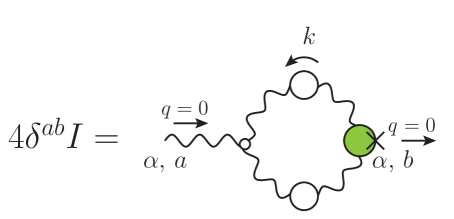
Figure 15.2: Diagrammatic definition of the scalar form factor, $I$, of the transition amplitude.

16 SDE of the pole-free vertex in the soft-gluon limit

It turns out that the soft-gluon limit of the SDE that controls the pole-free component, $\Gamma_{\alpha\mu\nu}^{abc}(q,r,p)$, of the three-gluon vertex is of central importance for the determination of the gluon mass scale. Indeed, as we will see in detail in Sec. 20, its judicious use leads to substantial simplifications at the level of the renormalized gluon mass equation. In order to clarify this important facet, we consider the SDE represented in Fig. 16.1, composed only by the tree-level contribution $(a_{1})$ and the diagram ($a_{2}$); diagrams where the gluon with momentum $q$ couples to a ghost-gluon or a four-gluon vertex are omitted. The reason why diagram ($a_{2}$) is singled out is because its kernel ${\cal K}$ appears also in the BSE for $\mathbb{B}(r^{2})$, shown in Fig. 18.1; as we will see, this fact is instrumental for the implementation of the renormalization procedure illustrated in Sec. 20.

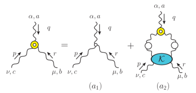
Figure 16.1: SDE for the regular part of the three-gluon vertex, $\Gamma^{abc}_{\alpha\mu\nu}(q,r,p)$, after the implementation of the skeleton expansion.

In the standard version of this SDE, the three-gluon vertex in diagram $(a_{2})$ is kept at tree level. The form employed here, with the three-gluon vertex fully-dressed, corresponds to the version of this SDE after the skeleton expansion has been implemented [274, 106]. Equivalently, this version of the SDE corresponds to the equation of motion for the vertex obtained within the formalism of the 3-particle irreducible effective action at three-loops [204, 208, 209, 275, 211, 216]. Consequently, the diagrammatic expansion of the kernel $\cal K$, given in Fig. 16.2, does not contain certain classes of diagrams (e.g., ladder graphs) in order to avoid overcounting. In fact, with the exception of the ghost loops, the diagrams of Fig. 16.2 comprise exactly the kernel of the standard glueball BSE [63, 66, 68].

The main advantage of this SDE is that the additional fully-dressed vertex absorbs the vertex renormalization $Z_{3}$, defined in Eq. (2.35), which otherwise would be multiplying the tree-level vertex. This is technically very advantageous, because, as we will see in the next section, the renormalization may be carried out subtractively rather than multiplicatively.

We now set $\Gamma_{\alpha\mu\nu}^{abc}(q,r,p)=f^{abc}\Gamma_{\alpha\mu\nu}(q,r,p)$, and evaluate the soft gluon limit of the SDE by substituting $q=0$ into Fig. 16.1. In particular, we find

$$f^{abc}\Gamma_{\alpha\mu\nu}(0,r,-r)=f^{abc}\Gamma_{\!0\,\alpha\mu\nu}(0,r,-r)\,+\,f^{amn}\int_{k}\Gamma_{\alpha\gamma\delta}(0,k,-k)\Delta^{\gamma\rho}(k)\Delta^{\delta\sigma}(k){\cal K}^{mnbc}_{\rho\sigma\mu\nu}(-k,k,r,-r)\,.$$ (16.1)

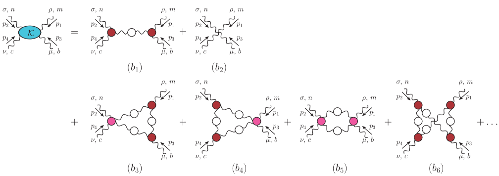
Figure 16.2: Skeleton expansion of the scattering kernel, ${\cal K}^{mnbc}_{\rho\sigma\mu\nu}(p_{1},p_{2},p_{3},p_{4})$. The one-gluon exchange is highlighted and the ellipsis denotes contributions with two or more loops.

We next consider the contraction of $\Gamma_{\alpha\mu\nu}(0,r,-r)$ by $P_{\mu^{\prime}}^{\mu}(r)P_{\nu^{\prime}}^{\nu}(r)$; the resulting projection is described in terms of a single form factor, denoted by $\mathit{L}_{{sg}}(r^{2})$, to wit [23, 146]

$$P_{\mu^{\prime}}^{\mu}(r)P_{\nu^{\prime}}^{\nu}(r)\Gamma_{\alpha\mu\nu}(0,r,-r)=2\mathit{L}_{{sg}}(r^{2})r_{\alpha}P_{\mu^{\prime}\nu^{\prime}}(r)\,.$$ (16.2)

Note, in fact, that, in the Landau gauge that we employ, the $\Gamma_{\alpha\gamma\delta}(0,k,-k)$ on the r.h.s. of Eq. (16.1) is automatically contracted by two transverse projectors, thus triggering Eq. (16.2) therein. Therefore, contracting both sides of Eq. (16.1) by $P^{\mu}_{\mu^{\prime}}(r)P^{\nu}_{\nu^{\prime}}(r)$, we obtain

$$f^{abc}\mathit{L}_{{sg}}(r^{2})r_{\alpha}P_{\mu^{\prime}\nu^{\prime}}(r)=f^{abc}r_{\alpha}P_{\mu^{\prime}\nu^{\prime}}(r)-f^{amn}\int_{k}k_{\alpha}\mathit{L}_{{sg}}(k^{2})\Delta^{2}(k^{2})P^{\rho\sigma}(k){\cal K}^{mnbc}_{\rho\sigma\mu\nu}(-k,k,r,-r)P^{\mu}_{\mu^{\prime}}(r)P^{\mu}_{\mu^{\prime}}(r)\,.$$ (16.3)

The last step is to contract Eq. (16.3) by $f^{abc}r^{\alpha}g^{\mu^{\prime}\nu^{\prime}}$, in order to eliminate the color and Lorentz indices. Introducing the strong charge $\alpha_{s}=g^{2}/4\pi$, using that $P^{\mu}_{\mu}(r)=3$, and that for SU($N$), $f^{abc}f^{abc}=C_{\rm A}(N^{2}-1)$, we finally arrive at

$$\mathit{L}_{{sg}}(r^{2})=\,1+\alpha_{s}\!\int_{k}k^{2}\Delta^{2}(k^{2})\,{K}(r,k)\,\mathit{L}_{{sg}}(k^{2})\,,$$ (16.4)

where the kernel $K(r,k)$ is defined as

$$\alpha_{s}K(r,k):=-\frac{(r\cdot k)}{c\,r^{2}k^{2}}f^{abc}f^{amn}P^{\mu\nu}(r)P^{\rho\sigma}(k)\,{\cal K}^{mnbc}_{\rho\sigma\mu\nu}(-k,k,r,-r)\,,$$ (16.5)

The numerical factor $c:=3C_{\rm A}(N^{2}-1)$ arises from the projections of Lorentz and color indices; for $N=3$, $c=72$.

17 Renormalization: general considerations

We now turn to a pivotal aspect of this analysis, and illustrate in detail the renormalization of the main dynamical components that arise from the activation of the Schwinger mechanism. In particular, we will elaborate on the renormalization properties of the key quantities $I$ and $B_{\mu\nu}$.

We begin by recalling that the gluon propagator and three-gluon vertex are renormalized by the constants $Z_{A}$ and $Z_{3}$, defined in Eq. (2.35), which are related to the gauge coupling renormalization constant, $Z_{g}$, through Eq. (2.36). Moreover, we will introduce two additional renormalization constants, to be denoted by $Z_{I}$ and $Z_{B}$, which renormalize the quantities $I$ and $B^{\mu\nu}(q,r,p)$, respectively. In particular [276],

$$I_{{\scriptscriptstyle R}}=Z^{-1}_{I}I\,,\quad\quad B_{{\scriptscriptstyle R}}^{\mu\nu}(q,r,p)=Z^{-1}_{B}B^{\mu\nu}(q,r,p)\,.$$ (17.1)

The partial derivatives of $B^{\mu\nu}(q,r,p)$ also renormalize in the same way, namely

$${\cal B}_{{\scriptscriptstyle R}}^{\alpha\mu\nu}(0,r,-r)=Z^{-1}_{B}{\cal B}_{{\scriptscriptstyle R}}^{\alpha\mu\nu}(0,r,-r)\,,\quad\quad\mathbb{B}_{{\scriptscriptstyle R}}(r^{2})=Z^{-1}_{B}\mathbb{B}(r^{2})\,.$$ (17.2)

Since both $I$ and $B^{\mu\nu}$ are comprised by the fundamental QCD components, it is natural to expect that both $Z_{I}$ and $Z_{B}$ can eventually be expressed in terms of the $Z_{A}$ and $Z_{3}$ introduced in Eq. (2.35). In fact, it is straightforward to deduce that [276]

$$Z_{I}=Z^{-1}_{3}Z_{A}\,,\quad\quad\quad Z_{B}=Z^{-1}_{A}\,.$$ (17.3)

To see how the relations in Eq. (17.3) arise, let us first consider Eq. (14.8). Since $m^{2}:=\Delta^{-1}(0)$, from the first relation in Eq. (2.35) we have that [276, 98]

$$m^{2}=Z^{-1}_{A}m^{2}_{{\scriptscriptstyle R}}\,.$$ (17.4)

On the other hand, combining Eq. (14.8), the first relation in Eq. (17.1), and Eq. (2.36), we find

$$m^{2}=g^{2}I^{2}=Z^{2}_{g}\,Z^{2}_{I}\,\underbrace{g^{2}_{{\scriptscriptstyle R}}I^{2}_{{\scriptscriptstyle R}}}_{m^{2}_{{\scriptscriptstyle R}}}=Z^{2}_{3}\,Z^{-3}_{A}\,Z^{2}_{I}\,m^{2}_{{\scriptscriptstyle R}}\,.$$ (17.5)

Then, the direct comparison of Eqs. (17.4) and (17.5) leads immediately to the first relation of Eq. (17.3).

The second relation of Eq. (17.3) may be obtained from Eq. (15.12), by recognizing that, since $V_{\alpha\mu\nu}(q,r,p)$ is a component of the three-gluon vertex ${\rm{I}}\!\Gamma^{\alpha\mu\nu}(q,r,p)$, it is renormalized according to Eq. (2.35), namely

$$V^{\alpha\mu\nu}(q,r,p)=Z^{-1}_{3}\,V^{\alpha\mu\nu}_{\!\!{\scriptscriptstyle R}}(q,r,p)\,,$$ (17.6)

and, consequently,

$${\mathbb{C}}(k^{2})=Z^{-1}_{3}\,{\mathbb{C}}_{\!{\scriptscriptstyle R}}(k^{2})\,.$$ (17.7)

On the other hand, from Eq. (15.12), using Eq. (17.1) and the first relation of Eq. (17.3), we get

$${\mathbb{C}}(k^{2})=-Z_{I}Z_{B}\underbrace{I_{{\scriptscriptstyle R}}\mathbb{B}_{{\scriptscriptstyle R}}(k^{2})}_{-{\mathbb{C}}_{\!{\scriptscriptstyle R}}(k^{2})}=Z^{-1}_{3}Z_{A}Z_{B}\,{\mathbb{C}}_{\!{\scriptscriptstyle R}}(k^{2})\,.$$ (17.8)

Then, the comparison between Eqs. (17.7) and (17.8) yields directly the second relation of Eq. (17.3).

We now address the renormalization of the kernel ${\cal K}^{mnbc}_{\rho\sigma\mu\nu}(q,r,p,t)$, which appears in Eq. (16.1), and later on in Eq. (18.4). We start by recognizing that ${\cal K}$ is a part of the four-gluon amplitude ${\cal G}^{mnbc}_{\rho\sigma\mu\nu}(q,r,p,t)$, which, in terms of gauge fields is given by ${\cal G}^{mnbc}_{\rho\sigma\mu\nu}(q,r,p,t)=\langle 0|T[\widetilde{A}^{m}_{\rho}(q)\widetilde{A}^{n}_{\sigma}(r)\widetilde{A}^{b}_{\mu}(p)\widetilde{A}^{c}_{\nu}(t)]|0\rangle$, but with the external legs amputated, i.e.,

$${\cal G}(q,r,p,t)=\Delta(q^{2})\Delta(r^{2})\Delta(p^{2})\Delta(t^{2}){\cal K}(q,r,p,t)+\cdots$$ (17.9)

where the ellipsis indicates the diagrams excluded when passing from the SDE to the BSE kernel, as explained in Sec. 16. Since, $A^{a\mu}_{{\scriptscriptstyle R}}=Z^{1/2}_{A}A^{a\mu}$, the above definition of ${\cal G}$ in terms of gauge fields implies that ${\cal G}_{{\scriptscriptstyle R}}=Z^{-2}_{A}\,{\cal G}$. Therefore, from Eqs. (17.9) and (2.35), we get

$${\cal K}_{{\scriptscriptstyle R}}(q,r,p,t)=Z^{2}_{A}\,{\cal K}(q,r,p,t)\,,$$ (17.10)

and, since ${\cal K}\sim\alpha_{s}K$, we arrive at

$${K}_{{\scriptscriptstyle R}}(q,r,p,t)=Z^{2}_{A}Z^{2}_{g}\,{K}(q,r,p,t)\,.$$ (17.11)

With the aid of the above relations, it is easy to prove that the combinations $\Delta{\mathbb{B}}$, $\Delta^{2}{\cal K}$, and $\alpha_{s}\Delta^{2}K$ are renormalization-group invariant (RGI), i.e.,

$$\Delta\mathbb{B}=\Delta_{{\scriptscriptstyle R}}\mathbb{B}_{{\scriptscriptstyle R}}\,,\qquad\qquad\Delta^{2}{\cal K}=\Delta^{2}_{{\scriptscriptstyle R}}\,{\cal K}_{{\scriptscriptstyle R}}\,,\qquad\qquad\alpha_{s}\Delta^{2}K=\alpha_{s}^{{\scriptscriptstyle R}}\Delta^{2}_{{\scriptscriptstyle R}}K_{{\scriptscriptstyle R}}\,.$$ (17.12)

As a self-consistency check, note that, by virtue of the renormalization rule $B_{{\scriptscriptstyle R}}^{\mu\nu}=Z_{A}B^{\mu\nu}$, given by Eqs. (17.1) and (17.3), the kernel ${\mathcal{M}}$ defined in Eq. (14.5) renormalizes as ${\cal M}_{{\scriptscriptstyle R}}=Z^{2}_{A}\,{\cal M}$, i.e., exactly as the kernel ${\mathcal{K}}$ in Eq. (17.10); this is precisely as expected, given that both ${\mathcal{K}}$ and ${\mathcal{M}}$ are parts of the same four-gluon kernel, see Eq. (14.4) and Fig. 14.3.

Capitalizing on the above results, we may now derive a useful expression for the $I_{{\scriptscriptstyle R}}$, using Eq. (15.16) as our point of departure. Specifically, substituting the bare quantities entering in Eq. (15.16) by renormalized ones, we have

$$4Z_{I}I_{{\scriptscriptstyle R}}=-\frac{iC_{\rm A}}{2}Z^{2}_{A}Z_{B}\int_{k}\Gamma_{\!0}^{\alpha\beta\lambda}(0,k,-k)\Delta_{{{\scriptscriptstyle R}}\,\beta}^{\mu}(k)\Delta_{{{\scriptscriptstyle R}}\,\lambda}^{\nu}(k)\,{\cal B}_{\!{{\scriptscriptstyle R}}\,\alpha\mu\nu}(0,-k,k)\,,$$ (17.13)

and, after employing Eq. (17.3),

$$4I_{{\scriptscriptstyle R}}=-\frac{iC_{\rm A}}{2}Z_{3}\int_{k}\Gamma_{\!0}^{\alpha\beta\lambda}(0,k,-k)\Delta_{{{\scriptscriptstyle R}}\,\beta}^{\mu}(k)\Delta_{{{\scriptscriptstyle R}}\,\lambda}^{\nu}(k)\,{\cal B}_{\!{{\scriptscriptstyle R}}\,\alpha\mu\nu}(0,-k,k)\,,$$ (17.14)

or, from Eq. (15.18),

$$I_{{\scriptscriptstyle R}}=-\frac{3iC_{\rm A}}{2}Z_{3}\int_{k}k^{2}\Delta_{{\scriptscriptstyle R}}^{2}(k^{2})\mathbb{B}_{{\scriptscriptstyle R}}(k^{2})\,.$$ (17.15)

We conclude this section with the renormalization of the SDE given in Eq. (16.4). By virtue of Eq. (16.2), it is clear that $\mathit{L}_{{sg}}^{\!{\scriptscriptstyle R}}(r^{2})=Z_{3}\mathit{L}_{{sg}}(r^{2})$; then, using Eq. (17.12), it is straightforward to show that the renormalized version of Eq. (16.4) reads

$$\mathit{L}_{{sg}}^{\!{\scriptscriptstyle R}}(r^{2})=\,Z_{3}+\alpha_{s}^{{\scriptscriptstyle R}}\!\!\int_{k}k^{2}\Delta^{2}_{{\scriptscriptstyle R}}(k^{2})\,{K}_{{\scriptscriptstyle R}}(r,k)\,\mathit{L}_{{sg}}^{\!{\scriptscriptstyle R}}(k^{2})\,.$$ (17.16)

As emphasized in Sec. 16, the renormalization required for Eq. (17.16) is subtractive.

Note finally that, in order to simplify the notation, in what follows we will drop the indices “R” from all renormalized equations.

18 Bethe-Salpeter equation for Schwinger pole formation

We now turn to one of the main dynamical issues associated with the generation of a gluonic mass scale, namely the BSE satisfied by the amplitude $\mathbb{B}(r^{2})$. The structure of this BSE turns out to be decisive for the success of the entire endeavor, not only because it admits nontrivial solutions for $\mathbb{B}(r^{2})$, but also because it is instrumental for the successful and concise implementation of the renormalization program. In this presentation we follow the construction developed in [100], where the non-linear structure of the BSE is fully retained ; for earlier, linearized versions of the same equation see [96, 97, 98, 144, 146].

The diagrammatic form of the BSE for the effective vertex $B_{\mu\nu}(q,r,p)$ is shown in the left part of Fig. 18.1, where the four-gluon kernel ${\cal T}$ is depicted in Fig. 14.2. In particular, from the first equality of Fig. 18.1 we have

$$B^{abc}_{\mu\nu}(q,r,p)=(G_{\cal T})^{abc}_{\mu\nu}(q,r,p)\,,$$ (18.1)

where

$$(G_{\cal T})^{abc}_{\mu\nu}(q,r,p)=\int_{k}B^{axe}_{\alpha\beta}(q,k,-t)\Delta_{xm}^{\alpha\rho}(k)\Delta_{en}^{\beta\sigma}(t){\cal T}^{mnbc}_{\rho\sigma\mu\nu}(-k,t,r,p)\,,$$ (18.2)

with $t:=k+q$. Then, after using Eqs. (14.4) and (14.5), two distinct terms appear, namely

$$(G_{\cal T})^{abc}_{\mu\nu}(q,r,p)=(G_{\cal K})^{abc}_{\mu\nu}(q,r,p)+(G_{\!{\cal M}})^{abc}_{\mu\nu}(q,r,p)\,,$$ (18.3)

with

$$(G_{\cal K})^{abc}_{\mu\nu}(q,r,p) = \int_{k}B^{axe}_{\alpha\beta}(q,k,-t)\Delta_{xm}^{\alpha\rho}(k)\Delta_{en}^{\beta\sigma}(t){\cal K}^{mnbc}_{\rho\sigma\mu\nu}(-k,t,r,p)\,,$$

$$(G_{\!{\cal M}})^{abc}_{\mu\nu}(q,r,p) = \Omega^{ad}(q)D^{ds}_{\Phi}(q)B^{sbc}_{\mu\nu}(q,r,p)\,,$$ (18.4)

where (symmetry factor $\frac{1}{2}$ included)

$$\Omega^{ad}(q)=\frac{1}{2}\int_{k}B^{axe}_{\alpha\beta}(q,k,-t)\Delta_{xm}^{\alpha\rho}(k)\Delta_{en}^{\beta\sigma}(t)B^{dnm}_{\sigma\rho}(-q,t,-k)\,.$$ (18.5)

Note that, while the term $(G_{\cal K})$ is linear in $B^{abc}_{\mu\nu}$, the term $(G_{\!{\cal M}})$ is cubic.

The first key step in the treatment of this BSE is to show that the product $\Omega^{ad}(q)D^{ds}_{\Phi}(q)$ appearing in $(G_{\!{\cal M}})$ is finite and nonvanishing as $q\to 0$. This is indeed so, because, in that limit, $\Omega^{ad}(q)\sim q^{2}\delta^{ad}$, thus canceling exactly the massless pole contained in $D^{ds}_{\Phi}(q)$.

To demonstrate this important result, set first $\Omega^{ad}(q)=\delta^{ad}\Omega(q^{2})$ in Eq. (18.5), and carry out the color algebra to obtain

$$\Omega(q^{2})=\frac{C_{\rm A}}{2}\int_{k}B_{\alpha\beta}(q,k,-t)P^{\alpha\rho}(k)P^{\beta\sigma}(t)B_{\rho\sigma}(-q,-k,t)\Delta(k^{2})\Delta(t^{2})\,.$$ (18.6)

Then, taking the limit $q\to 0$ of Eq. (18.6) using Eq. (15.11), we find

$$\lim_{q\to 0}\Omega(q^{2}) = \frac{C_{\rm A}}{2}\int_{k}{B}_{\alpha\beta}(0,k,-k)P^{\alpha\rho}(k)P^{\beta\sigma}(k){B}_{\sigma\rho}(0,k,-k)\Delta^{2}(k^{2})$$ (18.7)

$$= 6C_{\rm A}\int_{k}(q\cdot k)^{2}\Delta^{2}(k^{2})\mathbb{B}^{2}(k^{2})\,,$$

and consequently

$$\lim_{q\to 0}\Omega(q^{2})=q^{2}{\widetilde{\omega}}\,,\qquad\qquad{\widetilde{\omega}}:=\frac{3C_{\rm A}}{2}\int_{k}k^{2}\Delta^{2}(k^{2})\mathbb{B}^{2}(k^{2})\,.$$ (18.8)

Armed with this result, it is straightforward to establish that

$$(G_{\!{\cal M}})^{abc}_{\mu\nu}(0,r,-r)=\omega\,{B}_{\mu\nu}^{abc}(0,r,-r)\,,\qquad\omega:=i\,{\widetilde{\omega}}\,.$$ (18.9)

Evidently, the term in Eq. (18.9) may be carried to the l.h.s of Eq. (18.1), and combine directly with the term $B^{abc}_{\mu\nu}(q,r,p)$, in the same kinematic limit. In particular, after introducing the new variable,

$$\tau:=1-\omega\,,$$ (18.10)

Eq. (18.1) becomes

$$\tau\,{B}^{abc}_{\mu\nu}(0,r,-r)=\int_{k}B^{axe}_{\alpha\beta}(0,k,-k)\Delta_{xm}^{\alpha\rho}(k)\Delta_{en}^{\beta\sigma}(k){\cal K}^{mnbc}_{\rho\sigma\mu\nu}(-k,k,r,-r)\,.$$ (18.11)

It is clear now that, because of the validity of Eq. (15.3), Eq. (18.11) yields to lowest order a trivial result ($0=0$). Therefore, in order to obtain nontrivial dynamical information from Eq. (18.11), one must equate the terms linear in $q$ on both of its sides. In particular, using Eq. (15.4) for the $B_{\mu\nu}(0,r-r)$ and $B_{\alpha\beta}(0,k-k)$, one obtains the equationEq. (18.11)

$${\cal B}^{abc}_{\lambda\mu\nu}(0,r,-r)=\tau^{-1}\int_{k}{\cal B}^{axe}_{\lambda\alpha\beta}(0,k,-k)\Delta_{xm}^{\alpha\rho}(k)\Delta_{en}^{\beta\sigma}(k){\cal K}^{mnbc}_{\rho\sigma\mu\nu}(-k,k,r,-r)\,,$$ (18.12)

which admits the diagrammatic representation given in the second line of Fig. 18.1. Note that, in passing from Eq. (18.11) to Eq. (18.12), we have assumed that $\tau\neq 0$; of course, if $\tau=0$, the l.h.s. of Eq. (18.11) vanishes, and the remaining equation is no longer of the BSE type.

We now contract both sides by $P_{\mu^{\prime}}^{\mu}(r)P_{\nu^{\prime}}^{\nu}(r)$ and employ Eq. (15.7), to get

$$f^{abc}\,\mathbb{B}(r^{2})\,r_{\lambda}P_{\mu^{\prime}\nu^{\prime}}(r)\,=-\tau^{-1}f^{amn}\int_{k}\mathbb{B}(k^{2})\,\Delta^{2}(k^{2})\,k_{\lambda}P^{\sigma\rho}(k)\,{\cal K}^{mnbc}_{\rho\sigma\mu\nu}(-k,k,r,-r)P_{\mu^{\prime}}^{\mu}(r)P_{\nu^{\prime}}^{\nu}(r)\,.$$ (18.13)

Then, contracting both sides by $f^{abc}\,r^{\lambda}g^{\mu^{\prime}\nu^{\prime}}$, and using that $P_{\mu}^{\mu}(r)=3$, we arrive at the final BSE for the central quantity $\mathbb{B}(r^{2})$, namely

$$\mathbb{B}(r^{2})=\tau^{-1}\alpha_{s}\int_{k}k^{2}\Delta^{2}(k^{2}){K}(r,k)\mathbb{B}(k^{2})\,;$$ (18.14)

note that $K(r,k)$ is precisely the kernel introduced in Eq. (16.5).

Our final important observation regarding Eq. (18.14) is that it is RGI. This property may be easily established, by observing that, due to the first relation in Eq. (17.12), ${\widetilde{\omega}}$ itself, given by Eq. (18.8), is RGI, and so is the $\tau$ in Eq. (18.10), i.e.,

$$\omega=\omega_{{\scriptscriptstyle R}}\,,\qquad\tau=\tau_{{\scriptscriptstyle R}}\,.$$ (18.15)

Then, the BSE in Eq. (18.14) is RGI by virtue of the third relation in Eq. (17.12), and the fact that the $Z_{B}$, introduced to renormalize the $\mathbb{B}$, cancels on both sides. Consequently, one may substitute into Eq. (18.14) directly bare for renormalized quantities, without any renormalization constants appearing in the final expression, to wit

$$\mathbb{B}_{{\scriptscriptstyle R}}(r^{2})=\tau_{{\scriptscriptstyle R}}^{-1}\alpha_{s}^{{\scriptscriptstyle R}}\int_{k}k^{2}\Delta_{{\scriptscriptstyle R}}^{2}(k^{2}){K}_{{\scriptscriptstyle R}}(r,k)\mathbb{B}_{{\scriptscriptstyle R}}(k^{2})\,.$$ (18.16)

As before, the indices “R” will be omitted in what follows.

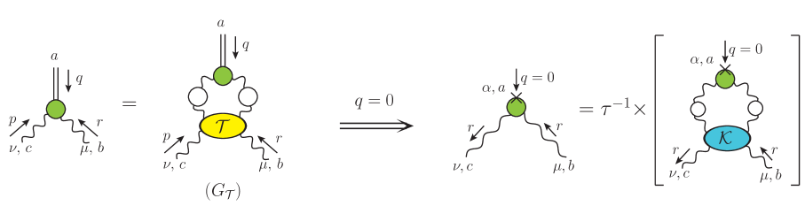
Figure 18.1: BSE for the effective vertex $B^{abc}_{\mu\nu}(q,r,p)$ (left), and its $q=0$ limit (right).

19 Dynamical scale-fixing of the BSE solutions

In order to proceed further with our analysis, certain key equations, derived in Minkowski space, must be converted to Euclidean space. This conversion is accomplished following the set of rules given in the App. A; applying them to Eqs. (17.15), (18.8), and (18.9), the expressions for $\omega_{{\rm{\scriptscriptstyle E}}}$ and $I_{{\rm{\scriptscriptstyle E}}}$ read

$$\omega_{{\rm{\scriptscriptstyle E}}} = \,\frac{3C_{\rm A}}{2}\int_{k_{{\rm{\scriptscriptstyle E}}}}k_{{\rm{\scriptscriptstyle E}}}^{2}\Delta^{2}_{{\rm{\scriptscriptstyle E}}}(k_{{\rm{\scriptscriptstyle E}}}^{2})\mathbb{B}_{{\rm{\scriptscriptstyle E}}}^{2}(k_{{\rm{\scriptscriptstyle E}}}^{2})\,,$$ (19.1)

$$I_{{\rm{\scriptscriptstyle E}}} = \,\frac{3C_{\rm A}Z_{3}}{2}\int_{k_{{\rm{\scriptscriptstyle E}}}}k_{{\rm{\scriptscriptstyle E}}}^{2}\Delta^{2}_{{\rm{\scriptscriptstyle E}}}(k_{{\rm{\scriptscriptstyle E}}}^{2})\mathbb{B}_{{\rm{\scriptscriptstyle E}}}(k_{{\rm{\scriptscriptstyle E}}}^{2})\,.$$ (19.2)

The Euclidean versions of Eqs. (17.16) and (18.16) may be derived in a similar way. In doing so, note that the kernel $K$ must be cast into the form

$$K(r,k)=iK_{{\rm{\scriptscriptstyle E}}}(r_{{\rm{\scriptscriptstyle E}}},k_{{\rm{\scriptscriptstyle E}}})\,,$$ (19.3)

where

$$i\,\alpha_{s}K_{{\rm{\scriptscriptstyle E}}}(r_{{\rm{\scriptscriptstyle E}}},k_{{\rm{\scriptscriptstyle E}}}):=\frac{(r_{{\rm{\scriptscriptstyle E}}}\cdot k_{{\rm{\scriptscriptstyle E}}})}{c\,r^{2}_{{\rm{\scriptscriptstyle E}}}k^{2}_{{\rm{\scriptscriptstyle E}}}}f^{abc}f^{amn}\left[P^{\mu\nu}(r)P^{\rho\sigma}(k)\,{\cal K}^{mnbc}_{\rho\sigma\mu\nu}(-k,k,r,-r)\right]_{{\rm{\scriptscriptstyle E}}}\,,$$ (19.4)

and $\left[\ldots\right]_{{\rm{\scriptscriptstyle E}}}$ denotes the transformation of the expressions in square brackets to Euclidean space. The origin of the factor “$i$” in Eq. (19.4) is easily understood at the level of the one-gluon exchange diagram $(b_{1})$ in Fig. 16.2, being included in the definition of the gluon propagator, see item (i) of Sec. 2.

Then, with $\tau_{{\rm{\scriptscriptstyle E}}}:=1-\omega_{{\rm{\scriptscriptstyle E}}}$, we have

$$\mathbb{B}_{{\rm{\scriptscriptstyle E}}}(r_{{\rm{\scriptscriptstyle E}}}^{2})=\tau_{{\rm{\scriptscriptstyle E}}}^{-1}\alpha_{s}\int_{k_{{\rm{\scriptscriptstyle E}}}}k_{{\rm{\scriptscriptstyle E}}}^{2}\Delta_{{\rm{\scriptscriptstyle E}}}^{2}(k_{{\rm{\scriptscriptstyle E}}}^{2}){K}_{{\rm{\scriptscriptstyle E}}}(r_{{\rm{\scriptscriptstyle E}}},k_{{\rm{\scriptscriptstyle E}}})\mathbb{B}_{{\rm{\scriptscriptstyle E}}}(k_{{\rm{\scriptscriptstyle E}}}^{2})\,,$$ (19.5)

whereas the equation for $\mathit{L}_{{sg}}^{{\rm{\scriptscriptstyle E}}}(r)$ becomes

$$\mathit{L}_{{sg}}^{\!{{\rm{\scriptscriptstyle E}}}}(r_{{\rm{\scriptscriptstyle E}}}^{2})=\,Z_{3}+\alpha_{s}\!\int_{k_{{\rm{\scriptscriptstyle E}}}}k_{{\rm{\scriptscriptstyle E}}}^{2}\Delta_{{\rm{\scriptscriptstyle E}}}^{2}(k_{{\rm{\scriptscriptstyle E}}}^{2})\,{K}_{{\rm{\scriptscriptstyle E}}}(r_{{\rm{\scriptscriptstyle E}}},k_{{\rm{\scriptscriptstyle E}}})\,\mathit{L}_{{sg}}^{\!{{\rm{\scriptscriptstyle E}}}}(k_{{\rm{\scriptscriptstyle E}}}^{2})\,.$$ (19.6)

Finally, the expressions for the Euclidean displacement function and mass retain the same form as in Eqs. (14.8) and (15.12), but now carry indices “E”, i.e.,

$${\mathbb{C}}_{{\rm{\scriptscriptstyle E}}}(r_{{\rm{\scriptscriptstyle E}}}^{2}):=-I_{{\rm{\scriptscriptstyle E}}}\,\mathbb{B}_{{\rm{\scriptscriptstyle E}}}(r_{{\rm{\scriptscriptstyle E}}}^{2})\,,$$ (19.7)

and

$$m^{2}_{{\rm{\scriptscriptstyle E}}}=g^{2}I^{2}_{{\rm{\scriptscriptstyle E}}}\,.$$ (19.8)

In order to simplify the notation, in what follows the index “E” will be dropped.

Let us now focus on the BSE of Eq. (19.5). Strictly speaking, it is a non-linear integral equation, due to the quadratic dependence of $\tau$ on the unknown function $\mathbb{B}(r^{2})$. Nonetheless, the fact that $\tau$ is a constant, independent of the variable $r$, allows one to convert the BSE into an eigenvalue problem, as is typical for linear homogeneous equations. There is, however, a crucial, and very welcome difference: the solutions do not suffer from a scale indeterminacy, as happens in the case of linear equations, where the multiplication of a given solution by an arbitrary number is also a solution. The reason for this decisive difference is precisely the presence of the parameter $\tau$, which fixes the scale, up to an overall sign.

In order to fully appreciate the function of $\tau$ in this context, we temporarily set $\tau=1$ inside Eq. (19.5). Then, suppose that the kernel $K$ is such that the eigenvalue that yields a nontrivial solution for $\mathbb{B}(k^{2})$ requires that $\alpha_{s}\to\alpha_{\star}$, where $\alpha_{\star}$ differs from the value predicted for $\alpha_{s}$ within the renormalization scheme employed.

Let us now restore $\tau$ at the level of Eq. (19.5); it is then clear that $\tau$ has to compensate exactly for the difference between $\alpha_{s}$ and $\alpha_{\star}$. Specifically, one must have

$$\tau=\frac{\alpha_{s}}{\alpha_{\star}}\,,$$ (19.9)

which converts Eq. (19.5) into the familiar form

$$\mathbb{B}(r^{2})=\alpha_{\star}\int_{k}k^{2}\Delta^{2}(k^{2}){K}(r,k)\mathbb{B}(k^{2})\,.$$ (19.10)

To understand how the presence of the parameter $\tau$ in Eq. (19.10) leads to the determination of the scale of $\mathbb{B}(k^{2})$, note that, by combining Eqs. (18.10) and (19.9), we obtain the condition

$$\omega=1-\alpha_{s}/\alpha_{\star}\,.$$ (19.11)

Since the value of the l.h.s. of Eq. (19.11) is fixed, the parameter $\omega$ is completely determined. Therefore, the size (scale) of the $\mathbb{B}(k^{2})$ entering in the definition of Eq. (19.1) is constrained: it has to be chosen such that both sides of Eq. (19.1) become equal.

To see how this works, let $\mathbb{B}_{0}(k^{2})$ represent a solution of Eq. (18.16) with a scale set arbitrarily, e.g., by imposing that the global maximum of $\mathbb{B}_{0}(k^{2})$ is at $1$. In addition, denote by $\omega_{0}$ the value of $\omega$ when $\mathbb{B}(k^{2})\to\mathbb{B}_{0}(k^{2})$ is substituted in Eq. (19.1). The $\mathbb{B}$ that is compatible with Eq. (19.11) is related to the $\mathbb{B}_{0}$ by a multiplicative constant, $\sigma$, i.e., $\mathbb{B}(k^{2})=\sigma\,\mathbb{B}_{0}(k^{2})$, whose value is determined from the equation

$$\sigma^{2}\omega_{0}=1-\alpha_{s}/\alpha_{\star}=\omega\,,$$ (19.12)

or, equivalently,

$$\sigma=\pm\sqrt{\frac{1-\alpha_{s}/\alpha_{\star}}{{\omega}_{0}}}=\pm\sqrt{\frac{\omega}{{\omega}_{0}}}\,.$$ (19.13)

Note that, since ${\omega}$ is quadratic in $\mathbb{B}(k^{2})$, the sign of $\sigma$, and hence the sign of $\mathbb{B}$ itself, is left undetermined. However, as we can see from Eqs. (19.2) and (19.7), ${\mathbb{C}}(k^{2})$ is also quadratic in $\mathbb{B}(k^{2})$, and therefore does not get affected by the sign ambiguity of Eq. (19.13). In fact, the overall sign of ${\mathbb{C}}(k^{2})$ turns out to be negative for the entire range of Euclidean momenta, in agreement with the sign found in the lattice extraction of ${\mathbb{C}}(k^{2})$ presented in [146, 148] [see also comments below Eq. (8.16), item (${\it i}$)].

20 An exceptional cancellation

Let us assume that the BS amplitude $\mathbb{B}(r^{2})$ has become available by solving the BSE in Eq. (19.10), and one would like to proceed with the determination of the gluon mass scale, by employing Eq. (19.8) in conjunction with Eq. (19.2). At that point, one is faced with the typical difficulty associated with the implementation of multiplicative renormalization: on the r.h.s. of Eq. (19.2) the integral is multiplied by the renormalization constant $Z_{3}$.

It turns out that a subtle set of circumstances allows one to implement the multiplicative renormalization at the level of Eq. (19.2) exactly. The final result amounts to the effective replacement $Z_{3}\to\omega\mathit{L}_{{sg}}(k^{2})$, i.e.,

$$I=\frac{3C_{\rm A}}{2}\omega\int_{k}k^{2}\Delta^{2}(k^{2})\mathit{L}_{{sg}}(k^{2})\mathbb{B}(k^{2})\,.$$ (20.1)

In what follows we will present a detailed derivation of the above important result.

The first main observation is that, thanks to Eq. (17.16), the $Z_{3}$ in Eq. (17.15) may be substituted by the combination

$$Z_{3}=\,\mathit{L}_{{sg}}(k^{2})-\alpha_{s}\!\!\int_{\ell}\ell^{2}\Delta^{2}(\ell^{2})\,{K}(k,\ell)\,\mathit{L}_{{sg}}(\ell^{2})\,.$$ (20.2)

This procedure is typically employed when dealing with multiplicative renormalizability at the level of the SDEs, see, e.g., [274], and is intimately connected with the “skeleton expansion” of the SDE kernel [274, 106].

The second observation is specific to the particular form of the BSE in Eq. (19.5): when the substitution of Eq. (20.2) is carried out, the BSE of Eq. (19.5) is formed inside Eq. (19.2), leading to a crucial cancellation, and, finally, to Eq. (20.1).

The essence of this cancellation may be captured by means of a simple toy example. In particular, consider two functions, $g(x)$ and $f(x)$, satisfying the system of integral equations

$$g(x)=z+\int\!\!dy\,\tilde{g}(y)K(x,y)\,,\qquad\qquad f(x)=b^{-1}\!\int\!\!dy\,\tilde{f}(y)K(x,y)\,,$$ (20.3)

where $\tilde{g}(y):=g(y)\,u(y)$ and $\tilde{f}(y):=f(y)\,u(y)$, with $u(y)$ a well-behaved function. The parameters $z$ and $b$ are real numbers, with $b\neq 0,1$, and the limits of integration are arbitrary. In addition, the common kernel $K(x,y)$ satisfies the symmetry relation $K(x,y)=K(y,x)$. Moreover, let us further assume that the value of a constant $\beta$ is given by the integral

$$\beta=z\!\int\!\!dx\,\tilde{f}(x)\,.$$ (20.4)

Observe now that the dependence of $\beta$ on the parameter $z$ may be eliminated in favor of the function $g(x)$ by resorting to the system of Eq. (20.3). Specifically, one employs the following sequence of steps

$$\beta = \int\!\!dx\,z\,\tilde{f}(x)$$ (20.5)

$$= \int\!\!dx\left[g(x)-\int\!\!dy\,\tilde{g}(y)K(x,y)\right]\tilde{f}(x)$$

$$= \int\!\!dx\,g(x)\tilde{f}(x)-\int\!\!dx\!\!\int\!\!dy\,\tilde{g}(y)K(x,y)\tilde{f}(x)$$

$$= \int\!\!dx\,\tilde{g}(x)\Bigg{[}f(x)-\underbrace{\int\!\!dy\,\tilde{f}(y)K(x,y)}_{bf(x)}\Bigg{]}\,,$$

where in the second line we used the first relation in Eq. (20.3), while in the last line the relabelling $x\leftrightarrow y$ of the integration variables was implemented, the symmetry of the kernel $K(x,y)$ was exploited, and the second relation in Eq. (20.3) was used. Thus, we find

$$\beta=(1-b)\int\!\!dx\tilde{f}(x)g(x)\,,$$ (20.6)

where we used that $\tilde{g}(x)f(x)=\tilde{f}(x)g(x)$. Clearly, the dependence of $\beta$ on the parameter $z$ has been exchanged in favor of the dependence on the function $g(x)$, which was absent from the original integral in Eq. (20.4). For a concrete example, where the equivalence between Eqs. (20.4) and (20.6) has been worked out explicitly, the reader is referred to the Appendix A of [100].

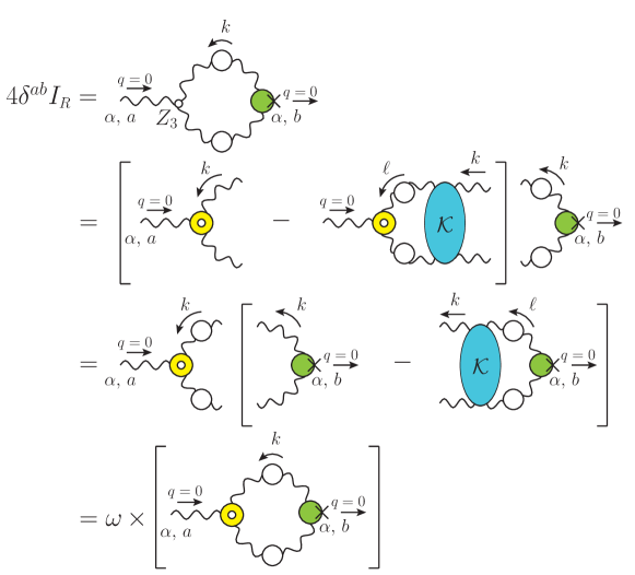
Figure 20.1: Diagrammatic illustration of the renormalization of $I$. Note that the diagrams containing the kernel ${\cal K}$ undergo a relabeling of integration momenta, $k\leftrightarrow\ell$, from the second to the third line.

It is now rather straightforward to repeat the construction leading to Eq. (20.6) for the system of integral equations given by Eqs. (19.5) and (19.6), in conjunction with Eq. (19.2); indeed, all we need is to establish the correspondence

$$\{g(x),\,f(x),\,u(x),\,K(x,y)\}\, \leftrightarrow\,\{\mathit{L}_{{sg}}(r^{2}),\,\mathbb{B}(r^{2}),\,k^{2}\Delta^{2}(k^{2}),\,\alpha_{s}K(r,k)\}\,,\,\,$$

$$\{\beta,\,z,\,b,\,dx,\,dy\}\, \leftrightarrow\,\{2I/3C_{\rm A},\,Z_{3},\,\tau,\,d^{4}k,\,d^{4}\ell\}\,.$$ (20.7)

In fact, with the above identifications and Eq. (18.10), we find that the analogue of Eq. (20.6) is precisely Eq. (20.1), which is the announced result. The diagrammatic representation of the steps described in Eq. (20.5) is shown in Fig. 20.1; note that, in doing so, we employ the representation of the BSE given in Fig. 18.1, whose main building block was introduced in Fig. 15.1.

The above construction exposes a remarkable fact: if the parameter $\omega$ is set to zero, the cancellation described in Eq. (20.5) [Fig. 20.1] is perfect. Therefore, even if a non-trivial $\mathbb{B}$ is obtained from Eq. (19.5), the renormalized transition amplitude $I$, and with it the gluon mass $m$, vanish. In that sense, the gluon mass emerges thanks to the mismatch between the kernels in the equations for $\mathbb{B}$ and $\mathit{L}_{{sg}}(r^{2})$, [see Eqs. (19.5) and (19.6)], which is caused by the presence of a $t\neq 1$ in the former but not in the latter. In diagrammatic terms, the nonvanishing of the gluon mass becomes possible due to the difference between the ${\cal T}$ appearing in Fig. 18.1 and the ${\cal K}$ in Fig. 16.1, namely the component ${\cal M}$ [see Fig. 14.2], which carries the vital information about the formation of the Schwinger pole.

21 Gluon mass versus Fredholm alternatives theorem

It turns out that the cancellations described in Eq. (20.5) are not accidental, but are rather enforced by an underlying mathematical principle. In particular, as we discuss in detail in this section, we have unveiled a rather subtle application of the so-called “Fredholm alternatives theorem”.

Consider the inhomogeneous and homogeneous Fredholm equations of the second kind, given by [150, 151]

$$f_{1}(x)=f_{2}(x)+\lambda\int_{a}^{b}K(x,y)f_{1}(y)dy\,,$$ (21.1)

and

$$f_{3}(x)=\lambda\int_{a}^{b}K(x,y)f_{3}(y)dy\,,$$ (21.2)

respectively; $f_{1}$ and $f_{3}$ are the unknown functions, while $f_{2}$ is a known inhomogeneous term. The kernel, $K(x,y)$, is assumed to be continuous and square-integrable in the interval $[a,b]$, in which case it is denominated a “Hilbert-Schmidt integral operator”.

The Fredholm alternatives theorem imposes restrictions on the existence of simultaneous solutions for Eqs. (21.1) and (21.2). It is sufficient for our purposes to consider the special case of the theorem when $K(x,y)$ is real and symmetric in $x\leftrightarrow y$; for the generalization to complex and non-symmetric kernels see, e.g., [150, 151]. Under these simplifications, the Fredholm alternatives theorem may be stated as follows [151]:

1. If $\lambda$ is not an eigenvalue of $K(x,y)$, i.e., if the homogeneous equation has only the trivial solution, $f_{3}(x)=0$, then the inhomogeneous Eq. (21.1) has a solution for any nonzero $f_{2}(x)$.

2. If $\lambda$ is an eigenvalue of $K(x,y)$, such that $f_{3}(x)$ is nonvanishing, then Eq. (21.1) has solutions if and only if

   $$\int_{a}^{b}f_{2}(y)f_{3}(y)dy=0\,.$$ (21.3)

In order to expose the connection between the Fredholm alternative theorem and the system of equations satisfied by $\mathit{L}_{{sg}}(r^{2})$ and $\mathbb{B}(r^{2})$, we need to perform certain transformations that will cast Eqs. (19.5) and (19.6) into a form similar to Eqs. (21.1) and (21.2).

The first step is to rewrite Eqs. (19.5) and (19.6) in hyperspherical coordinates, using the variables introduced in Eq. (A.5). Note that the kernel $K(r,k)$ is a function of $x$, $y$, and $\theta$, i.e., $K(r,k)\equiv K(x,y,\theta)$. Furthermore, we use the integral measure of Eq. (A.6), which introduces an ultraviolet regulator to control potential divergences of the integrals. For the sake of simplicity we employ a hard momentum cutoff, $\Lambda$; we have confirmed that exactly the same conclusions are reached when the calculation is carried out using dimensional regularization. So, the integral measure takes the form

$$\int_{k}:=\frac{1}{(2\pi)^{3}}\int_{0}^{\Lambda^{2}}\!\!dy\,y\int_{0}^{\pi}\!\!d\theta\,s_{\theta}^{2}\,.$$ (21.4)

Now, the only dependence of the integrands of Eqs. (19.5) and (19.6) on the angle is through $K(x,y,\theta)$. Then, we can define an “angle-integrated kernel”, ${\widehat{K}}(x,y)$, by

$${\widehat{K}}(x,y)=\frac{1}{(2\pi)^{3}}\!\int_{0}^{\pi}\!\!d\theta\,s_{\theta}^{2}\,K(x,y,\theta)\,.$$ (21.5)

With the above definitions, Eqs. (19.5) and (19.6) are recast as

$$\mathbb{B}(x)= \,\tau^{-1}\alpha_{s}\!\int_{0}^{\Lambda^{2}}\!\!dy\,{\cal Z}^{2}(y){\widehat{K}}(x,y)\mathbb{B}(y)\,,$$

$$\mathit{L}_{{sg}}(x)= \,Z_{3}+\alpha_{s}\!\int_{0}^{\Lambda^{2}}\!\!dy\,{\cal Z}^{2}(y){\widehat{K}}(x,y)\mathit{L}_{{sg}}(y)\,,$$ (21.6)

where we introduced the gluon dressing function, ${\cal Z}(x):=x\Delta(x)$, first defined in Eq. (2.23).

We next note that, since $K(r,k)$ is symmetric under the exchange of $r\leftrightarrow k$, then ${\widehat{K}}(x,y)={\widehat{K}}(y,x)$. However, the complete kernel of Eq. (21.6), namely ${\cal Z}^{2}(y){\widehat{K}}(x,y)$, is not symmetric under $x\leftrightarrow y$, due to the factor of ${\cal Z}^{2}(y)$. Nonetheless, we can easily transform it into an equivalent system of equations with a symmetric kernel, by multiplying Eq. (21.6) by ${\cal Z}(x)$, and defining

$${\widetilde{\mathbb{B}}}(x):={\cal Z}(x)\mathbb{B}(x)\,,\qquad{\widetilde{L}}_{sg}(x):={\cal Z}(x)\mathit{L}_{{sg}}(x)\,,\qquad{\widetilde{K}}(x,y):={\cal Z}(x){\cal Z}(y){\widehat{K}}(x,y)\,.$$ (21.7)

Then, Eq. (21.6) is equivalent to

$${\widetilde{\mathbb{B}}}(x)= \,\tau^{-1}\alpha_{s}\!\int_{0}^{\Lambda^{2}}\!\!dy\,{\widetilde{K}}(x,y){\widetilde{\mathbb{B}}}(y)\,,$$

$${\widetilde{L}}_{sg}(x)= \,Z_{3}{\cal Z}(x)+\alpha_{s}\!\int_{0}^{\Lambda^{2}}\!\!dy\,{\widetilde{K}}(x,y){\widetilde{L}}_{sg}(y)\,,$$ (21.8)

whose kernel ${\widetilde{K}}(x,y)$ is indeed symmetric.

Finally, Eq. (19.2) for $I$ may be re-expressed as

$$I=\frac{3C_{\rm A}Z_{3}}{32\pi^{2}}\!\int_{0}^{\Lambda^{2}}\!\!dy\,{\cal Z}(y)\,{\widetilde{\mathbb{B}}}(y)\,.$$ (21.9)

We are now in position to explore the implications of Fredholm’s alternatives theorem for Eq. (21.8). Specifically, suppose that $\omega=0$, such that $\tau=1$. Then, we have a direct correspondence between Eq. (21.8) and the Eqs. (21.1) and (21.2) through the identification

$$\{f_{1}(x),\,f_{2}(x),\,f_{3}(x),\,K(x,y)\}\, \leftrightarrow\,\{{\widetilde{L}}_{sg}(x),\,Z_{3}{\cal Z}(x),\,{\widetilde{\mathbb{B}}}(x),\,{\widetilde{K}}(x,y)\}\,,$$

$$\{\lambda,\,a,\,b\}\, \leftrightarrow\,\{\alpha_{s},\,0,\,{\Lambda^{2}}\}\,.$$ (21.10)

Hence, for both $\mathit{L}_{{sg}}(x)$ and $\mathbb{B}(x)$ to be nonzero, the Fredholm alternatives theorem implies that

$$Z_{3}\int_{0}^{\Lambda^{2}}\!\!dy\,{\cal Z}(y)\,{\widetilde{\mathbb{B}}}(y)=0\,.$$ (21.11)

Comparison to Eq. (21.9) then yields $I=0$, and therefore, due to Eq. (14.8), $m^{2}=0$.

We thus reach the conclusion that the generation of a gluon mass scale through the Schwinger mechanism hinges on $\omega\neq 0$, $\tau\neq 1$, which leads to the evasion of Fredholm alternatives theorem, by relaxing the equality of kernels in Eq. (21.8). Instead, if $\omega=0$, the theorem imposes the vanishing of the gluon mass, even in the presence of a nonvanishing $\mathbb{B}$; this happens because, quite remarkably, the condition of Eq. (21.3) is precisely the equation for the transition amplitude $I$.

We finally address a subtlety related to the applicability of Fredholm’s theorem in the present situation. Note, in particular, that the kernel $K(r,k)$ depends on $\mathit{L}_{{sg}}(r^{2})$, through every three-gluon appearing in the defining diagrams of Fig. 16.2; in fact, the $\mathit{L}_{{sg}}$ enters in $K(r,k)$ in such a way that the symmetry under $r\longleftrightarrow k$ is preserved. As a result, the integral equation for $\mathit{L}_{{sg}}(r^{2})$ [second in Eq. (21.6)] is nonlinear (even when $\omega=0$), while Fredholm’s theorem applies to a system of linear equations. However, our main conclusion, namely that for $\omega=0$ the gluon mass scale vanishes, persists.

Indeed, suppose that there exists a solution, $L_{0}(r^{2})$ and $\mathbb{B}_{0}(r^{2})$, to the full nonlinear system of equations, and let $K_{0}(r,k)$ be the value of $K(r,k)$ obtained by the substitution of $\mathit{L}_{{sg}}\to L_{0}$ in its expression. Now, $L_{0}(r^{2})$ and $\mathbb{B}_{0}(r^{2})$ must also be a solution of

$$\mathit{L}_{{sg}}(r^{2})= \,Z_{3}+\alpha_{s}\!\int_{k}k^{2}\Delta^{2}(k^{2})\,{K}_{0}(r,k)\,\mathit{L}_{{sg}}(k^{2})\,,$$

$$\mathbb{B}(r^{2})= \,\tau^{-1}\alpha_{s}\!\int_{k}k^{2}\Delta^{2}(k^{2})\,{K}_{0}(r,k)\,\mathbb{B}(k^{2})\,,$$ (21.12)

since setting $\{\mathit{L}_{{sg}},\,\mathbb{B}\}\to\{L_{0},\,\mathbb{B}_{0}\}$ in the above equation one recovers the original, nonlinear, system. But the Fredholm alternatives theorem applies to Eq. (21.12) with $\omega=0$, in which case the arguments of Sec. 21 lead to $m=0$. Consequently, the nonlinear nature of the equations cannot by itself evade the Fredholm alternatives theorem when $\omega=0$, and the conclusion of our analysis is unaffected.

22 Emergence of the gluon mass scale

The detailed analysis presented in the previous sections has led us to a set of dynamical equations, whose solutions will determine the value of the gluon mass scale that emerges from this approach. In this section we culminate this exploration by determining $m$, as well as the shape and size of the displacement function ${\mathbb{C}}(r^{2})$, following the procedure introduced in the recent work of [100]. In doing so, we use two important results as benchmarks for these quantities. Specifically, we identify as the optimal value for the gluon mass the inverse of the saturation point of the lattice gluon propagator at the origin; when the lattice curve has been renormalized such that $\Delta^{-1}(\mu^{2})=\mu^{2}$ at $\mu=4.3$ GeV, one finds $m_{{\rm{\scriptscriptstyle lat}}}=354$ MeV [23]. Similarly, the curve shown on the right panel of Fig. 12.2 is used as benchmark for the displacement function; in this section we will denote this curve by ${\mathbb{C}}_{{\rm{\scriptscriptstyle WI}}}(r^{2})$, where the subscript “WI” refers to the WI-based derivation of this result.

The procedure that we adopt for the computation of $m$ and ${\mathbb{C}}(r^{2})$ may be summarized as follows:

(${\it i}$) The relations given by Eqs. (19.10), (19.1) and (20.1) are written in terms of hyperspherical coordinates, employing the variables defined in Eq. (A.5). In particular,

$$\mathbb{B}(x) = \tau^{-1}\frac{\alpha_{s}}{(2\pi)^{3}}\int_{0}^{\infty}\!\!dy\,\int_{0}^{\pi}\!\!d\theta\,s_{\theta}^{2}\,{\cal Z}^{2}(y)K(x,y,\theta)\,\mathbb{B}(y)\,,$$ (22.1)

$$\omega = \,\frac{3C_{\rm A}}{32\pi^{2}}\int_{0}^{\infty}\!\!\!dy{\cal Z}^{2}(y)\,\mathbb{B}^{2}(y)\,,$$ (22.2)

$$I = \frac{3C_{\rm A}}{32\pi^{2}}\omega\int_{0}^{\infty}\!\!\!dy\,{\cal Z}^{2}(y)\,\mathit{L}_{{sg}}(y)\,\mathbb{B}(y)\,.$$ (22.3)

(${\it ii}$) For a given kernel, $K(x,y,\theta)$, the eigenvalue problem of Eq. (22.1) can be solved with standard procedures, such as Nyström’s method [277]. This determines the eigenvalue, $\alpha_{\star}$, and a solution, $\mathbb{B}_{0}(x)$, arbitrarily normalized such that its global maximum is $1$. Then, we use Eq. (19.12) to obtain the value of $\omega$ corresponding to this $\alpha_{\star}$.

(${\it iii}$) Next, we substitute $\mathbb{B}_{0}(x)$ into Eq. (22.2), thus obtaining the value of $\omega_{0}$. So, the physical scale of $\mathbb{B}(x)$ is fixed by determining the value of the constant $\sigma$ from Eq. (19.13).

(${\it iv}$) We may now determine the value of $I$, by substituting into Eq. (22.3) the $\mathbb{B}(x)$ obtained in the previous step.

(${\it v}$) Finally, with the $I$ determined in (${\it iv}$), we can get $m$ and ${\mathbb{C}}(r^{2})$ using Eqs. (19.8) and (19.7), respectively.

The initial form that we will use for the four-gluon kernel $K(r,k)$ entering in the BSE of Eq. (19.5) is its one-gluon exchange approximation, $K_{\rm oge}(r,k)$, given by diagram $(b_{1})$ of Fig. 16.2; we remind the reader that diagram $(b_{2})$ vanishes when inserted in Eq. (19.4) [96, 144].

In the Landau gauge, we obtain from diagram $(b_{1})$ and Eq. (19.4)

$$K_{\rm oge}(r,k)=\frac{2\pi C_{\rm A}}{3}\Delta(u^{2})\left[\frac{(r\cdot k)}{r^{2}k^{2}}\overline{\Gamma}_{\mu\rho\sigma}(r,-k,u)\overline{\Gamma}^{\mu\rho\sigma}(-r,k,u)\right]_{{\rm{\scriptscriptstyle E}}}\,,$$ (22.4)

where $u:=k-r$, and

$$\overline{\Gamma}_{\mu\rho\sigma}(r,-k,u):=P^{\mu^{\prime}}_{\mu}(r)P^{\rho^{\prime}}_{\rho}(k)P^{\sigma^{\prime}}_{\sigma}(u){\rm{I}}\!\Gamma_{\mu^{\prime}\rho^{\prime}\sigma^{\prime}}(r,-k,u)\,,$$ (22.5)

is the transversely projected three-gluon vertex [214, 213, 278, 116, 117, 190, 251, 216, 99].

The $\overline{\Gamma}_{\mu\rho\sigma}$ appearing in Eq. (22.4) is described in terms of four independent tensor structures and the corresponding form factors, which depend on three kinematic variables. However, as has been shown in numerous studies [214, 213, 278, 116, 117, 190, 279, 251, 216, 99, 252], the classical tensor structure of $\overline{\Gamma}_{\mu\rho\sigma}$ is dominant. Moreover, the associated form factor, $\mathit{L}_{{sg}}$, may be accurately described as a function of a single kinematic variable, denoted by $s^{2}$, namely

$$\overline{\Gamma}^{\mu\rho\sigma}(r,-k,u)=\overline{\Gamma}_{\!0}^{\mu\rho\sigma}(r,-k,u)\mathit{L}_{{sg}}(s^{2})\,,\qquad s^{2}:=\frac{1}{2}[r^{2}+k^{2}+u^{2}]\,,$$ (22.6)

where $\overline{\Gamma}_{\!0}^{\mu\rho\sigma}$ is the tree-level value of $\overline{\Gamma}^{\mu\rho\sigma}$, obtained by substituting the ${\rm{I}}\!\Gamma^{\mu^{\prime}\rho^{\prime}\sigma^{\prime}}$ in Eq. (22.5) by the ${\rm{I}}\!\Gamma_{\!0}^{\mu^{\prime}\rho^{\prime}\sigma^{\prime}}$ of Eq. (2.26). This special property of the three-gluon vertex is known in the literature as “planar degeneracy” [251].

Then, using Eq. (22.6) and the variables of Eq. (A.5), one obtains

$$K_{\rm oge}(x,y,\theta)=K_{\rm{kin}}(x,y,\theta){\cal R}_{\rm oge}(u^{2},s^{2})\,,$$ (22.7)

where we note that $u^{2}=x+y-2c_{\theta}\sqrt{xy}$, $s^{2}=x+y-c_{\theta}\sqrt{xy}$,

$$K_{\rm{kin}}(x,y,\theta):=\frac{8\pi C_{\rm A}}{3u^{2}\sqrt{xy}}\left\{c_{\theta}s_{\theta}^{2}\left[(c_{\theta}^{2}+8)xy-6c_{\theta}\sqrt{xy}(x+y)+3(x^{2}+y^{2})\right]\right\}\,,$$ (22.8)

and

$${\cal R}_{\rm oge}(u^{2},s^{2}):={\Delta(u^{2})\mathit{L}_{{sg}}^{2}(s^{2})}\,.$$ (22.9)

The ingredients entering in the $K_{\rm oge}(x,y,\theta)$ of Eq. (22.7) are all accurately known from lattice simulations. In particular, we use for $\Delta(u^{2})$ and $\mathit{L}_{{sg}}(s^{2})$ the fits to the lattice results of [23], given by Eqs. (C.11) and (C.12) of [146], respectively; the corresponding curves are shown in Fig. 12.1. $\Delta(u^{2})$ is also shown on the upper left panel of Fig. 22.1, for the purpose of comparison with the modified version, $\Delta^{\prime}(u^{2})$, introduced later in Eq. (22.14).

Note that these ingredients are renormalized within the so-called “asymmetric MOM scheme” [186, 187, 188, 189, 182, 190, 23], defined by the renormalization condition [see App. B]

$$\Delta^{-1}(\mu^{2})=\mu^{2}\,,\qquad\mathit{L}_{{sg}}(\mu^{2})=1\,,$$ (22.10)

with $\mu=4.3$ GeV denoting the renormalization point. For this renormalization scheme and point, the corresponding strong charge takes the value $\alpha_{s}=0.27$ [189], which we adopt from now on.

On the upper right panel of Fig. 22.1 we show as an orange dashed curve the diagonal slice of the angle-integrated ${\widehat{K}}(x,y)$ [see Eq. (21.5)], namely ${\widehat{K}}(k^{2},k^{2})$.

Substituting into Eq. (22.1) the $K_{\rm oge}(x,y,\theta)$ given by Eqs. (22.7), (22.8) and (22.9), we find that $\alpha_{\star}=0.685$; the corresponding BS amplitude, to be denoted by $\mathbb{B}_{{\rm oge}}(r^{2})$, is shown as the orange dashed curve on the lower left panel of Fig. 22.1. Note that its asymptotic ultraviolet behavior is such that the integrals in Eqs. (22.2) and (22.3) are perfectly convergent. In particular, we find that the numerical solution for $\mathbb{B}_{{\rm oge}}(r^{2})$ may be accurately approximated by the form

$$\mathbb{B}_{{\rm oge}}(r^{2})=\frac{a}{r^{2}L_{{\rm{\scriptscriptstyle UV}}}^{\kappa}(r^{2})}\,,\qquad r>5~{\rm GeV}\,,$$ (22.11)

where $L_{{\rm{\scriptscriptstyle UV}}}(r^{2})$ is the function introduced in Eq. (8.18), while $a=3.93$ and $\kappa=0.958$ are determined by fitting the data of $\mathbb{B}_{{\rm oge}}(r^{2})$ for $r>5~{\rm GeV}$.

Then, following the steps (${\it ii}$)-(${\it iv}$), we obtain the gluon mass scale, whose value we denote by $m_{{\rm oge}}$; in particular we find $m_{{\rm oge}}=1.27$ GeV. Similarly, for the displacement functions, to be denoted by ${\mathbb{C}}_{{\rm oge}}(r^{2})$, we find the orange dashed curve shown on the lower right panel of Fig. 22.1. Evidently, both outcomes differ substantially from the benchmark results of $m_{{\rm{\scriptscriptstyle lat}}}=354$ MeV and the curve corresponding to ${\mathbb{C}}_{{\rm{\scriptscriptstyle WI}}}(r^{2})$.

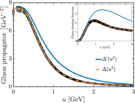
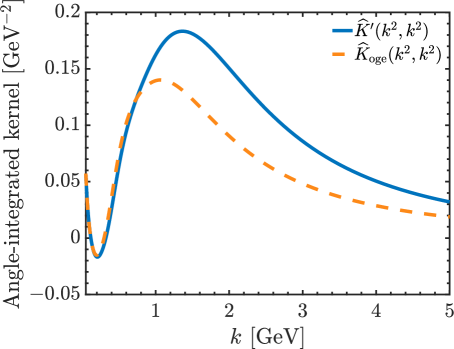
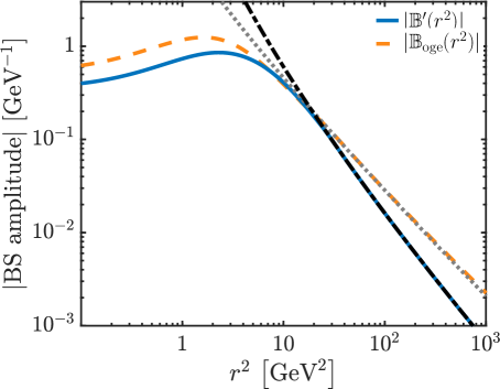
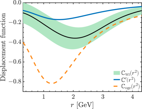
Figure 22.1: Upper left: The effective gluon propagator, corresponding to the two choices used in our analysis, namely $\Delta(u^{2})$ (orange dashed) and $\Delta^{\prime}(u^{2})$ (blue continuous); the inset shows the associated dressing functions. Upper right: The diagonal slice of the angle-integrated kernel, defined by Eq. (21.5); the orange dashed curve corresponds to ${\widehat{K}}_{\rm{oge}}(k^{2},k^{2})$, while the blue continuous to ${\widehat{K}}^{\prime}(k^{2},k^{2})$. Lower left: The absolute value of the BS amplitude; the orange dashed curve represents the $|\mathbb{B}_{\rm{oge}}(r^{2})|$, while the blue continuous curve denotes the |$\mathbb{B}^{\prime}(r^{2})|$. The black dot-dashed and gray dashed lines represent the corresponding asymptotes, given by Eq. (22.11). Lower right: Displacement amplitude; the orange dashed curve corresponds to ${\mathbb{C}}_{\rm oge}(r^{2})$, while the blue continuous denotes the ${\mathbb{C}}^{\prime}(r^{2})$. The black curve surrounded by the green band is displayed for comparison; it corresponds to the WI-derived result of Sec. 12 [see right panel of Fig. 12.2], denoted here by ${\mathbb{C}}_{{\rm{\scriptscriptstyle WI}}}(r^{2})$.

This discrepancy motivates the modification of the kernel $K(x,y,\theta)$, for the purpose of improving the results; evidently, the underlying idea is to effectively model contributions not captured by the one-gluon exchange approximation. To that end, we implement the substitution

$$K(x,y,\theta)\to K^{\prime}(x,y,\theta)=K_{\rm{kin}}(x,y,\theta){\cal R}^{\prime}(u^{2},s^{2})\,,$$ (22.12)

where the function ${\cal R}^{\prime}(u^{2},s^{2})$ is given by

$${\cal R}^{\prime}(u^{2},s^{2})=\Delta^{\prime}(u^{2})\mathit{L}_{{sg}}(s^{2})\,,$$ (22.13)

with $\Delta^{\prime}(u^{2})$ parametrized as

$$\Delta^{\prime}(u^{2})=\Delta(u^{2})\times\left[1+\frac{c_{0}u^{2}}{1+c_{1}u^{2}+c_{2}u^{4}}\right]\,.$$ (22.14)

Note that $K_{\rm oge}$ is recovered by setting $c_{0}=0$ in Eq. (22.14). Moreover, at large momenta, $\Delta^{\prime}(u^{2})$ reduces to $\Delta(u^{2})$, such that the $K^{\prime}$ so constructed reduces asymptotically to $K_{\rm oge}$.

We next vary the $c_{i}$ in Eq. (22.14) within certain intervals, and consider the resulting values for $m$. Our analysis reveals that the “optimal” set of values is given by $c_{0}=0.503$ GeV^-2, $c_{1}=0.00667$ GeV^-2 and $c_{2}=0.0486$ GeV^-4. The $\Delta^{\prime}(u^{2})$ and $\widehat{K}^{\prime}(k^{2},k^{2})$ obtained using this set of $c_{i}$ are shown as blue continuous curves on the upper left and upper right panels of Fig. 22.1, respectively. Substituting the $K^{\prime}(x,y,\theta)$ into the BSE of Eq. (22.1), we find that $\alpha_{\star}=0.414$. The corresponding solution, $\mathbb{B}^{\prime}(r^{2})$, is shown as the blue continuous curve on the lower left panel of Fig. 22.1; its asymptotic form is given by Eq. (22.11), with $\mathbb{B}_{{\rm oge}}\to\mathbb{B}^{\prime}$, and parameters given by $a=3.94$, and $\kappa=2.66$. The repetition of the steps (${\it ii}$)-(${\it iv}$) furnishes for the gluon mass scale the value $m^{\prime}=367$ MeV, which differs by only $3.6\%$ from $m_{{\rm{\scriptscriptstyle lat}}}=354$ MeV. The corresponding displacement function ${\mathbb{C}}^{\prime}(r^{2})$ is shown as the continuous blue curve on the lower right panel of Fig. 22.1. Evidently, the modification of the kernel implemented by Eq. (22.12) has reduced considerably the discrepancy between ${\mathbb{C}}^{\prime}(r^{2})$ and ${\mathbb{C}}_{{\rm{\scriptscriptstyle WI}}}(r^{2})$.

At this point we remind the reader that the determination of ${\mathbb{C}}_{{\rm{\scriptscriptstyle WI}}}(r^{2})$ in Sec. 12 uses lattice inputs for all ingredients except for the partial derivative ${\cal W}(r^{2})$, defined in Eq. (11.14). Indeed, ${\cal W}(r^{2})$ was obtained from the SDE analysis of App. F, using diagrams ($h_{1}$) and ($h_{2}$) of Fig. F.1, but omitting diagram ($h_{3}$), on the grounds of furnishing only a $\sim 2\%$ effect at the level of the ghost-gluon vertex, in the symmetric limit [280]. However, with hindsight, the partial derivative of a small form factor may be considerable, especially if the kinematic configuration studied is not the symmetric one.

The above considerations prompt us to determine the shape that ${\cal W}(r^{2})$ must have in order for ${\mathbb{C}}_{{\rm{\scriptscriptstyle WI}}}(r^{2})$ and ${\mathbb{C}}^{\prime}(r^{2})$ to coincide, ${\mathbb{C}}_{{\rm{\scriptscriptstyle WI}}}(r^{2})={\mathbb{C}}^{\prime}(r^{2})$. Denoting this ideal ${\cal W}(r^{2})$ by ${\cal W}^{\,\prime}(r^{2})$, it is clear that it can be obtained from Eq. (12.4), after substituting in it ${\mathbb{C}}(r^{2})\to{\mathbb{C}}^{\prime}(r^{2})$, namely

$${\cal W}^{\,\prime}(r^{2})=r^{2}\Delta(r^{2})\left[\frac{\mathit{L}_{{sg}}(r^{2})-{\mathbb{C}}^{\prime}(r^{2})}{F(0)}-{\widetilde{Z}}_{1}\frac{d\Delta^{-1}(r^{2})}{dr^{2}}\right]\,;$$ (22.15)

the result is shown as a purple dashed curve and band on the left panel of Fig. 22.2.

Now, given that the ingredients entering the diagrams $(h_{1})$ and $(h_{2})$ are firmly under control, this change in the shape of ${\cal W}(r^{2})$ can only be attributed to the contribution of diagram $(h_{3})$, namely

$${\cal W}_{3}(r^{2})={\cal W}^{\,\prime}(r^{2})-{\cal W}_{1}(r^{2})-{\cal W}_{2}(r^{2})\,.$$ (22.16)

Then, from our results for the ${\cal W}_{1}$, ${\cal W}_{2}$ and ${\cal W}^{\,\prime}$, we obtain the ${\cal W}_{3}(r^{2})$ that is shown as a blue continuous curve on the right panel of Fig. 22.2, where the associated band originates from propagating the statistical error of $\mathit{L}_{{sg}}(r^{2})$. Note that this ${\cal W}_{3}(r^{2})$ corresponds to a maximum change of $14\%$ of ${\cal W}(r^{2})$ at $r=2$ GeV.

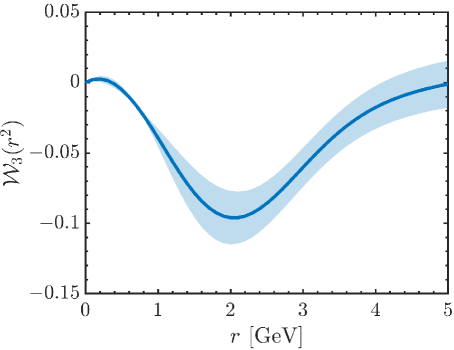
Figure 22.2: Left: The ${\cal W}(r^{2})$ obtained from the SDE analysis of App. F, using diagrams ($h_{1}$) and ($h_{2}$) of Fig. F.1 (blue continuous), and the ${\cal W}^{\,\prime}(r^{2})$ (purple-dashed), obtained from Eq. (22.15), enforcing ${\mathbb{C}}_{{\rm{\scriptscriptstyle WI}}}(r^{2})={\mathbb{C}}^{\prime}(r^{2})$. Right: The contribution ${\cal W}_{3}(r^{2})$ obtained from Eq. (22.16), expected to arise from diagram $(h_{3})$. For each curve in this figure, the band corresponds to the error propagated from the lattice $\mathit{L}_{{sg}}(r^{2})$.

23 Discussion and conclusions

The picture that emerges from the implementation of the Schwinger mechanism in QCD is rather appealing, especially in view of its ability to expose deep field-theoretic principles that are at work. In particular, the tight interplay between symmetry and dynamics is revealed by the multiple role played by the function ${\mathbb{C}}(r^{2})$, which is $({\it a})$ the residue function of the Schwinger poles, see Eq. (7.20); $({\it b})$ the displacement function of the Ward identity, see Eq. (11.16); and $({\it c})$ proportional to the BS amplitude that describes the formation of the massless excitations, see Eq. (19.7). The definitions and terminology employed throughout this article for the description of ${\mathbb{C}}(r^{2})$ are summarized for convenience in Table  23.1.

${\mathbb{C}}(r^{2})$
Defining equation	$\displaystyle{\lim_{q\to 0}}\frac{V_{1}(q,r,p)}{q^{2}}=\frac{2(q\cdot r)}{q^{2}}{\mathbb{C}}(r^{2})$	$\mathit{L}_{{sg}}(r^{2})=L_{0}(r^{2})+{\mathbb{C}}(r^{2})$	${\mathbb{C}}(r^{2})=-I\mathbb{B}(r^{2})$
Terminology	Residue function	Displacement function	Proportional to the BS amplitude

Table 23.1: Equivalent definitions of the function ${\mathbb{C}}(r^{2})$ and the corresponding terminology.

In addition, the combined treatment based on the functional equations (standard SDEs, SDEs within the PT-BFM framework, and the BSE for Schwinger pole formation) proves particularly successful in describing the dynamics, and, most importantly, in faithfully reflecting the action of key mathematical principles, such as the seagull cancellation [Sec. 5] and Fredholm’s alternatives theorem [Sec. 21].

It is also important to emphasize the fruitful synergy between continuous methods and lattice QCD, demonstrated throughout this work. In particular, lattice-derived inputs, such as gluon propagators and vertices, have been extensively used in our numerical analysis, both for the determination of the $m$ and ${\mathbb{C}}(r^{2})$ in Sec. 22, as well as the function ${\cal W}(r^{2})$ in App. F. In fact, this synergy reaches its culmination in Sec. 12, where the lattice-based determination of the displacement function ${\mathbb{C}}(r^{2})$ is carried out.

A particularly noteworthy feature of our analysis is the exact implementation of the multiplicative renormalization of Eq. (19.2), described in Sec. 20. This becomes possible due to the precise cancellation captured by Eq. (20.5), and represents a rare case where such an exact result may be reached in a nonperturbative context. In fact, the operation of Fredholm’s alternatives theorem at this level, together with its subsequent evasion thanks to the inclusion of the pole term proportional to $\omega$ [see Sec. 21], is exceptionally striking.

The aforementioned major cancellation of Sec. 20 was diagrammatically described with the aid of Fig. 20.1. In order to simplify the analysis, we have considered the minimum of diagrams required for exposing the gist of this cancellation, and its connection to Fredholm’s theorem, presented in Sec. 21. It is important to stress, however, that, as we have confirmed, the omitted contributions undergo themselves completely analogous cancellations, proceeding in exactly the same way, and for precisely the same reason. In fact, we have confirmed that the construction pertaining to the renormalization may be extended to include the ghost-gluon and four-gluon vertices, the renormalization constants associated with them, and the corresponding SDE-BSE systems. Quite interestingly, and in complete analogy to what we have seen, the only contributions that survive originate from the nonlinear components of the additional BSEs that control the formation of poles in the ghost-gluon and four-gluon vertices. Therefore, the generalization of Eq. (20.1) will involve additional terms proportional to the $\omega$-like parameters that will emerge exactly as in Eqs. (18.7) and (18.8).

It should be emphasized that the analysis of Sec. 22 is by no means exhaustive, and leaves considerable room for improvement. (${\it i}$) To begin with, in the diagrammatic representation of the four-gluon kernel $K(r,k)$ one must include a graph that exhibits the Schwinger pole, namely ($b_{1}$) but with the internal gluon replaced by the scalar field $\Phi$. This type of contribution was omitted from the initial analysis, but its impact must be assessed in a more detailed analysis. In fact, as was shown in [96] [see Fig. 20 therein], the presence of such graphs is essential for the decoupling of massless excitation from on-shell amplitudes. (${\it ii}$) In addition, the inclusions of the one-loop dressed diagrams ($b_{3}$)-($b_{6}$) appearing in the skeleton expansion of Fig. 16.2 must be duly taken into account. (${\it iii}$) Furthermore, motivated by the discussion presented at the end of Sec. 22, it would be important to study the possible numerical impact of graph ($h_{3}$) on the function ${\cal W}(r^{2})$. Given that this entails a two-loop calculation, the practical implementation of this point is rather challenging. (${\it iv}$) Finally, as mentioned above, the inclusion of the ghost-gluon and four-gluon vertices will modify the expression for $I$ given in Eq. (20.1), and may affect the overall numerical picture.

Throughout this article we have focused exclusively on the implementation of the Schwinger mechanism within the Landau gauge, $\xi=0$. It should be emphasized, however, that a detailed analysis carried out in [55] reveals that the mechanism persists at least within the interval $\xi\in[0,0.5]$. This picture is compatible with related studies [281, 282] involving the Nielsen identities [283, 284].

As has become clear from the analysis presented in this work, the formation of colored massless poles out of the fusion of two gluons or of a ghost-antighost pair is an indispensable condition for the generation of a gluon mass scale through the Schwinger mechanism. Quite interestingly, colored massless poles are also required for the nonperturbative realization of the BRST quartet mechanism [143, 285]; their generation is controlled by appropriate BSEs, exactly as happens in the case of the Schwinger poles. Despite these similarities, however, to date no conclusive connection has been established between these two mechanisms.

We end by pointing out that, among the plethora of states predicted by QCD, the glueballs [58, 59, 60, 61, 62, 63, 64, 65, 66, 67, 68] and hybrids [286, 287, 288, 289] contain “valence gluons”, and are thus expected to be sensitive to the gluon mass scale; the detection and classification of these states are among the primary goals of experiments such as BES III [290, 291] and GlueX [292, 293]. In fact, as asserted in [294], their discovery will lead to a paradigm-shifting reassessment of the distinction between matter field and force fields, since the massive gluons will be acting as both. The gluon mass scale is also likely to be important in understanding the production of heavy mesons, e.g., $J/\psi$ and $\phi$, from a proton target, as these processes are generally considered to be deeply connected to gluon physics [295, 296, 297, 298]. Finally, the gluon mass scale should leave signals in gluon distribution functions [299, 300], for which data obtained in the planned EIC [301] and EicC [302] facilities will provide valuable insights.

Appendix A Euclidean space conventions

In this Appendix we summarize the rules and conventions adopted throughout this work for transforming expressions from Minkowski to Euclidean space.

To begin with, for our numerical studies we consider all physical momenta to be space-like; in particular, $r^{2}\to-r_{{\rm{\scriptscriptstyle E}}}^{2}$, where $r_{{\rm{\scriptscriptstyle E}}}$ is an Euclidean momentum with $r_{{\rm{\scriptscriptstyle E}}}^{2}>0$, and similarly for other momenta. At the level of the integral measure of Eq. (3.17), this transformation entails

$$\int_{k}=i\int_{k_{{\rm{\scriptscriptstyle E}}}}\,.$$ (A.1)

Then, for the propagators and their dressing functions, we adopt the conventions

$$\Delta_{{\rm{\scriptscriptstyle E}}}(r_{{\rm{\scriptscriptstyle E}}}^{2})=\,-\Delta(-r_{{\rm{\scriptscriptstyle E}}}^{2})\,,\qquad D_{{\rm{\scriptscriptstyle E}}}(r_{{\rm{\scriptscriptstyle E}}}^{2})=\,-D(-r_{{\rm{\scriptscriptstyle E}}}^{2})\,,\qquad{\cal Z}_{{\rm{\scriptscriptstyle E}}}(r_{{\rm{\scriptscriptstyle E}}}^{2})=\,{\cal Z}(-r_{{\rm{\scriptscriptstyle E}}}^{2})\,,\qquad F_{{\rm{\scriptscriptstyle E}}}(r_{{\rm{\scriptscriptstyle E}}}^{2})=\,F(-r_{{\rm{\scriptscriptstyle E}}}^{2})\,.$$ (A.2)

Next, for the pole-free form factor of the three-gluon vertex in the soft-gluon limit, and the function ${\cal W}(r^{2})$, both appearing in the WI displacement of Eq. (12.4), we define

$$\mathit{L}_{{sg}}^{\!{{\rm{\scriptscriptstyle E}}}}(r_{{\rm{\scriptscriptstyle E}}}^{2})=\mathit{L}_{{sg}}(-r_{{\rm{\scriptscriptstyle E}}}^{2})\,,\qquad{\cal W}_{{\rm{\scriptscriptstyle E}}}(r_{{\rm{\scriptscriptstyle E}}}^{2})={\cal W}(-r_{{\rm{\scriptscriptstyle E}}}^{2})\,.$$ (A.3)

Lastly, due to the derivatives with respect to squared momenta in the definitions of the functions ${\mathbb{C}}(r^{2})$, ${\mathcal{C}}(r^{2})$ and $\mathbb{B}(r^{2})$ [see Eqs. (7.20), (7.22) and (15.8), respectively], they are transformed to Euclidean space as

$${\mathbb{C}}_{{\rm{\scriptscriptstyle E}}}(r_{{\rm{\scriptscriptstyle E}}}^{2})=-{\mathbb{C}}(-r_{{\rm{\scriptscriptstyle E}}}^{2})\,,\qquad{\mathcal{C}}_{{\rm{\scriptscriptstyle E}}}(r_{{\rm{\scriptscriptstyle E}}}^{2})=\,-{\mathcal{C}}(-r_{{\rm{\scriptscriptstyle E}}}^{2})\,,\qquad\mathbb{B}_{{\rm{\scriptscriptstyle E}}}(r_{{\rm{\scriptscriptstyle E}}}^{2})=-\mathbb{B}(-r_{{\rm{\scriptscriptstyle E}}}^{2})\,.$$ (A.4)

In order to evaluate the Euclidean integrals numerically, it is convenient to use hyperspherical coordinates. For the typical integrals encountered in this work, e.g., Eqs. (19.5) and (19.6), involving a single external momentum, $r_{{\rm{\scriptscriptstyle E}}}$, and a virtual momentum, $k_{{\rm{\scriptscriptstyle E}}}$, we introduce the variables

$$x:=r_{{\rm{\scriptscriptstyle E}}}^{2}\,,\qquad y:=k_{{\rm{\scriptscriptstyle E}}}^{2}\,,\qquad r_{{\rm{\scriptscriptstyle E}}}\cdot k_{{\rm{\scriptscriptstyle E}}}:=\sqrt{xy}c_{\theta}\,,$$ (A.5)

where $\theta$ is the angle between $r_{{\rm{\scriptscriptstyle E}}}$ and $k_{{\rm{\scriptscriptstyle E}}}$, and we write $c_{\theta}:=\cos\theta$ and $s_{\theta}:=\sin\theta$. Then, the integral measure becomes

$$\int_{k}=\frac{i}{(2\pi)^{3}}\int_{0}^{\Lambda^{2}}\!\!dy\,y\int_{0}^{\pi}\!\!d\theta s^{2}_{\theta}\,,$$ (A.6)

with a cutoff $\Lambda$ introduced for numerical purposes.

Appendix B The asymmetric MOM renormalization scheme

In this Appendix we introduce the renormalization scheme adopted throughout this work, namely the asymmetric MOM scheme [186, 187, 188, 189, 182, 190, 23].

For the pure Yang-Mills SU(3) that we consider, a renormalization scheme is specified by prescribing values for three of the renormalization constants in Eq. (2.35); all others are determined from the STIs, i.e., through Eq. (2.36) [183]. In the MOM type of renormalization schemes [183, 184, 185], this is achieved by imposing boundary conditions on the renormalized forms of three chosen Green functions.

Specifically, all MOM schemes require that the renormalized propagators assume tree-level values at the renormalization point $\mu$, i.e.,  [183, 184, 185]

$$\Delta^{-1}_{{\rm{\scriptscriptstyle R}}}(\mu^{2})=\mu^{2}\,,\qquad F_{{\rm{\scriptscriptstyle R}}}(\mu^{2})=1\,.$$ (B.1)

Then, the third renormalization constant is specified by imposing that the classical form factor of one of the fundamental vertices also reduces to tree-level at a specified kinematic configuration [183].

In Landau gauge studies, it is common to complete the renormalization prescription by adopting the so-called “Taylor scheme” [102, 258, 270, 271, 23]. This renormalization scheme takes advantage of the well-known Taylor theorem [102], which states that in Landau gauge the fully dressed unrenormalized ghost-gluon vertex reduces to tree-level in the soft-ghost configuration, i.e.,

$${\rm{I}}\!\Gamma_{\nu}(r,0,-r)=r_{\nu}\,.$$ (B.2)

The Taylor scheme is then defined by requiring that the renormalized ghost-gluon vertex also satisfies Eq. (B.2) [102, 258, 270, 271, 23]. Within this scheme, Eq. (2.35) implies that the ghost-gluon renormalization constant reduces to $Z_{1}=1$.

For the present work, where the soft-gluon form factor of the three-gluon vertex $\mathit{L}_{{sg}}(r^{2})$, defined in Eq. (12.1), plays a key role, it is more convenient to adopt a renormalization scheme defined by imposing a boundary condition on $\mathit{L}_{{sg}}(r^{2})$. Specifically, we impose that $\mathit{L}_{{sg}}(r^{2})$ reduces to tree-level at $r=\mu$, i.e.,

$$\mathit{L}_{{sg}}^{{\rm{\scriptscriptstyle R}}}(\mu^{2})=1\,.$$ (B.3)

Together, Eqs. (B.1) and (B.3) define the asymmetric MOM scheme, which has been extensively employed in nonperturbative studies of $\mathit{L}_{{sg}}(r^{2})$ [188, 189, 182, 190, 23, 252, 216].

In contrast to the Taylor scheme, in the asymmetric MOM scheme the finite ghost-gluon renormalization constant is no longer equal to $1$ [182, 23]. The value of this constant in the asymmetric MOM scheme, to be denoted by ${\widetilde{Z}}_{1}$, has been determined through SDE studies to be ${\widetilde{Z}}_{1}=0.9333\pm 0.0075$ [148] (see also Sec. 8 of [99]). Moreover, at the same value of the renormalization point, lattice simulations determine the renormalized coupling to be $\alpha_{s}(4.3\text{ GeV})=0.27$ [189].

We point out that other choices of vertices and/or configurations to define MOM-type renormalization schemes have been explored in the literature. Some examples include the “symmetric MOM scheme”, wherein the classical form factor of the three-gluon vertex reduces to tree level at the symmetric point, $q^{2}=r^{2}=p^{2}=\mu^{2}$ [188, 189, 190], and MOM type schemes defined by imposing a boundary condition on the four-gluon vertex [217, 218].

Appendix C The seagull cancellation in the Landau gauge

In the demonstration of the seagull cancellation in Subsec. 5.5, the value of the gauge-fixing parameter was left completely arbitrary; therefore, the main result captured by Eq. (5.43) is valid for general $\xi_{Q}$. Nevertheless, it is instructive to perform the derivation explicitly in the Landau gauge, for the purpose of elucidating a subtlety that arises within the PT-BFM framework. Specifically, as is clear from Eq. (5.37), the BQQ vertex, $\widetilde{\Gamma}_{\alpha\mu\nu}(q,r,p)$, is ill-defined in the Landau gauge: due to the presence of terms proportional to $\xi_{Q}^{-1}$, the limit $\xi_{Q}\to 0$ may not be taken directly. The correct procedure is to take this limit after the contraction $\Delta^{\rho\mu}(r)\Delta^{\sigma\nu}(p)\widetilde{\Gamma}_{\alpha\mu\nu}(q,r,p)$ has been carried out; then, one obtains a well-defined result, as we will now show.

There are two key observations that are relevant for this construction. First, the terms proportional to $\xi_{Q}^{-1}$ in $\widetilde{\Gamma}_{\alpha\mu\nu}(q,r,p)$ do not receive radiative corrections, retaining their tree-level form to all orders [180]. Specifically, we may write

$$\widetilde{{\rm{I}}\!\Gamma}_{\alpha\mu\nu}(q,r,p)=\widetilde{{\mathbf{\Gamma}}}\vphantom{\Gamma}_{\alpha\mu\nu}(q,r,p)+\xi_{Q}^{-1}(g_{\alpha\nu}r_{\mu}-g_{\alpha\mu}p_{\nu})\,,$$ (C.1)

where the $\xi_{Q}^{-1}$ term is identical to that of $\widetilde{\Gamma}_{\!0\,\alpha\mu\nu}(q,r,p)$ in Eq. (5.37), while $\widetilde{{\mathbf{\Gamma}}}\vphantom{\Gamma}_{\alpha\mu\nu}(q,r,p)$ is well-defined at $\xi_{Q}=0$. At tree-level, $\widetilde{{\mathbf{\Gamma}}}\vphantom{\Gamma}_{\!0\,\alpha\mu\nu}(q,r,p)=\widetilde{\Gamma}_{\!0\,\alpha\mu\nu}(q,r,p)$, and Eq. (5.37) is recovered. Moreover, it follows from Eqs. (4.3), (2.19) and (C.1), that the special vertex $\widetilde{{\mathbf{\Gamma}}}\vphantom{\Gamma}_{\alpha\mu\nu}(q,r,p)$ satisfies (for any $\xi_{Q}$) the STI [180]

$$q^{\alpha}\widetilde{{\mathbf{\Gamma}}}\vphantom{\Gamma}_{\alpha\mu\nu}(q,r,p)=\Delta^{-1}(p^{2})P_{\mu\nu}(p)-\Delta^{-1}(r^{2})P_{\mu\nu}(r)\,.$$ (C.2)

Second, the terms proportional to $\xi^{-1}_{Q}$ in Eq. (C.1) are longitudinal, namely proportional to $r_{\mu}$ and $p_{\nu}$; thus, when contracted with gluon propagators, $\Delta^{\rho\mu}(r)\Delta^{\sigma\nu}(p)$, they trigger the identity,

$$r_{\mu}\Delta^{\rho\mu}(r)=\xi_{Q}\frac{r^{\rho}}{r^{2}}\,.$$ (C.3)

As a result,

$$\Delta^{\rho\mu}(r)\Delta^{\sigma\nu}(p)\widetilde{\Gamma}_{\alpha\mu\nu}(q,r,p)=\Delta^{\rho\mu}(r)\Delta^{\sigma\nu}(p)\widetilde{{\mathbf{\Gamma}}}\vphantom{\Gamma}_{\alpha\mu\nu}(q,r,p)+\frac{r^{\rho}}{r^{2}}\Delta^{\sigma}_{\alpha}(p)-\frac{p^{\sigma}}{p^{2}}\Delta^{\rho}_{\alpha}(p)\,,$$ (C.4)

which is free of $\xi_{Q}^{-1}$ terms, and can be safely set to the Landau gauge value, wherein

$$\lim_{\xi_{Q}\to 0}\Delta^{\rho\mu}(r)\Delta^{\sigma\nu}(p)\widetilde{\Gamma}_{\alpha\mu\nu}(q,r,p)=\Delta(r^{2})\Delta(p^{2})P^{\rho\mu}(r)P^{\sigma\nu}(p)\widetilde{{\mathbf{\Gamma}}}\vphantom{\Gamma}_{\alpha\mu\nu}(q,r,p)+\frac{r^{\rho}}{r^{2}}P^{\sigma}_{\alpha}(p)\Delta(p^{2})-\frac{p^{\sigma}}{p^{2}}P^{\rho}_{\alpha}(r)\Delta(r^{2})\,.$$ (C.5)

Note that the last two terms originate from the product of a term proportional to $\xi_{Q}$, coming from a gluon propagator, and a term proportional to $\xi_{Q}^{-1}$, originating from $\widetilde{\Gamma}_{\alpha\mu\nu}(q,r,p)$.

Armed with these results, we may now demonstrate the seagull cancellation explicitly in the Landau gauge. Using Eq. (C.5), the self-energy terms ${\tilde{a}}_{1}$ and ${\tilde{a}}_{2}$ of Eqs. (5.34) and (5.35) can be expressed at $\xi_{Q}=0$ as

$${\tilde{a}}_{1}= \,\frac{g^{2}C_{\rm A}}{2d}\int_{k}\Gamma_{\!0\,\mu\alpha\beta}(0,k,-k)\left\{\Delta^{2}(k^{2})P^{\alpha\rho}(k)P^{\beta\sigma}(k)\widetilde{{\mathbf{\Gamma}}}\vphantom{\Gamma}^{\mu}_{\rho\sigma}(0,k,-k)+\frac{\Delta(k^{2})}{k^{2}}\left[k^{\alpha}P^{\beta\mu}(k)+k^{\beta}P^{\alpha\mu}(k)\right]\right\}\,,$$ (C.6)

$${\tilde{a}}_{2}= \,-g^{2}C_{\rm A}\frac{(d-1)^{2}}{d}\int_{k}\Delta(k^{2})\,.$$ (C.7)

Next, the STI of Eq. (C.2), together with the assumption that $\widetilde{{\mathbf{\Gamma}}}\vphantom{\Gamma}_{\alpha\mu\nu}(q,r,p)$ is pole free at $q=0$, imply the WI

$$\widetilde{{\mathbf{\Gamma}}}\vphantom{\Gamma}^{\mu}_{\rho\sigma}(0,k,-k)=\frac{\partial[\Delta^{-1}(k^{2})P_{\rho\sigma}(k)]}{\partial k_{\mu}}=-2k^{\mu}P_{\rho\sigma}(k)\Delta^{-2}(k^{2})\frac{\partial\Delta(k^{2})}{\partial k^{2}}-\frac{\Delta^{-1}(k^{2})}{k^{2}}\left(g^{\mu}_{\rho}k_{\sigma}+g^{\mu}_{\sigma}k_{\rho}-\frac{2k^{\mu}k_{\rho}k_{\sigma}}{k^{2}}\right)\,.$$ (C.8)

Note that the term in parenthesis is annihilated by the projectors $P^{\alpha\rho}(k)P^{\beta\sigma}(k)$ in Eq. (C.6), such that

$${\tilde{a}}_{1}=\frac{g^{2}C_{\rm A}}{2d}\int_{k}\Gamma_{\!0\,\mu\alpha\beta}(0,k,-k)\left\{-2k^{\mu}P^{\alpha\beta}(k)\frac{\partial\Delta(k^{2})}{\partial k^{2}}+\frac{\Delta(k^{2})}{k^{2}}\left[k^{\alpha}P^{\beta\mu}(k)+k^{\beta}P^{\alpha\mu}(k)\right]\right\}\,.$$ (C.9)

To complete the demonstration, we use that

$$k^{\mu}P^{\alpha\beta}(k)\Gamma_{\!0\,\mu\alpha\beta}(0,k,-k)=2(d-1)k^{2}\,,\qquad\left[k^{\alpha}P^{\beta\mu}(k)+k^{\beta}P^{\alpha\mu}(k)\right]\Gamma_{\!0\,\mu\alpha\beta}(0,k,-k)=-2(d-1)k^{2}\,,$$ (C.10)

which entail

$${\tilde{a}}_{1}=-\frac{2g^{2}C_{\rm A}(d-1)}{d}\left[\int_{k}k^{2}\frac{\partial\Delta(k^{2})}{\partial k^{2}}+\frac{1}{2}\int_{k}\Delta(k^{2})\right]\,.$$ (C.11)

Hence, combining the above with Eq. (C.7) yields

$${\widetilde{\Pi}}^{(1)}(0)={\tilde{a}}_{1}+{\tilde{a}}_{2}=-\frac{2g^{2}C_{\rm A}(d-1)}{d}\underbrace{\left[\int_{k}k^{2}\frac{\partial\Delta(k^{2})}{\partial k^{2}}+\frac{d}{2}\int_{k}\Delta(k^{2})\right]}_{\text{seagull identity}}=0\,,$$ (C.12)

where the seagull identity of Eq. (5.10) is once again triggered. We emphasize that the last two terms of Eq. (C.5), resulting from the subtle cancellation of the gauge-fixing parameter in the PT-BFM scheme, are crucial for the vanishing of ${\widetilde{\Pi}}^{(1)}(0)$.

Finally, as an alternative to the $\xi_{Q}$-independent demonstration of Subsec. 5.5, one may opt for repeating the above procedure for general $\xi_{Q}$. In that case, the terms quadratic in $\xi_{Q}$, present in Eq. (C.4), vanish when contracted with $\Gamma_{\!0\,\alpha\mu\nu}(0,k,-k)$ in Eq. (C.6). Then, after some algebra and the use of Eq. (C.8), the terms linear in $\xi_{Q}$, appearing in both ${\tilde{a}}_{1}$ and ${\tilde{a}}_{2}$, can be shown to be proportional to

$$\int_{k}\frac{1}{k^{2}}=0\,,$$ (C.13)

which is itself a special case of the seagull identity, with $\Delta(k^{2})=1/k^{2}$ and $d\neq 2$.

Appendix D SDE implementation of the seagull cancellation: an example

The implementation of the seagull cancellation at the level of the SDEs raises certain practical issues that deserve our attention. In particular, while the derivation of the seagull identity relies on the use of a regularization scheme that preserves the translational invariance of the integral, the numerical treatment of the SDEs employs typically a hard ultraviolet cutoff, which breaks this invariance. The way around this apparent difficulty is to implement the seagull at the level of the SDEs before the numerical treatment is initiated [95].

To see this in the simple context of scalar QED, consider the two integrals given in Eq. (5.18), and use for the vertex $\Gamma_{\nu}(-q,t,-k)$ an Ansatz that satisfies automatically the WTI of Eq. (5.19). In particular, we use the standard choice [303, 304]

$$\Gamma_{\nu}(-q,t,-k)=(t+k)_{\nu}{u}(q,k)\,,\qquad{u}(q,k):=\frac{{\cal D}^{-1}(t^{2})-{\cal D}^{-1}(k^{2})}{t^{2}-k^{2}}\,,$$ (D.1)

such that

$$(d_{1})_{\mu\nu}=e^{2}\int_{k}(t+k)_{\mu}(t+k)_{\nu}{\cal D}(k^{2}){\cal D}(t^{2})u(q,k)=-e^{2}\int_{k}(t+k)_{\mu}(t+k)_{\nu}f(q,k)\,,$$ (D.2)

where

$$f(q,k):=\frac{{\cal D}(t^{2})-{\cal D}(k^{2})}{t^{2}-k^{2}}\,,$$ (D.3)

while $(d_{2})_{\mu\nu}$ is given by the second integral in Eq. (5.18).

Evidently, at $q=0$,

$$f(0,k)=\frac{\partial{\cal D}(k^{2})}{\partial k^{2}}\,.$$ (D.4)

Then, since from Eq. (5.20) we have that

$$(d-1)\Pi^{(1)}(q^{2})=\Pi^{(1)\mu}_{\mu}(q)=(d_{1})_{\mu}^{\mu}+(d_{2})_{\mu}^{\mu}\,,$$ (D.5)

we find that

$$(d-1)\Pi^{(1)}(q^{2})=-e^{2}\left[\int_{k}(t+k)^{2}f(q,k)+2d\int_{k}{\cal D}(k^{2})\right]\,.$$ (D.6)

Using $(t+k)^{2}=4k^{2}-q^{2}+2(t^{2}-k^{2})$ and that $\int_{k}(t^{2}-k^{2})f(q,k)=0$, we find

$$(d-1)\Pi^{(1)}(q^{2})=-e^{2}\left[\int_{k}(4k^{2}-q^{2})f(q,k)+2d\int_{k}{\cal D}(k^{2})\right]\,.$$ (D.7)

Setting $q=0$ into Eq. (D.7), and using Eq. (D.4), we recover immediately the seagull identity of Eq. (5.25).

Note at this point that if the r.h.s. of Eq. (D.7) were to be computed numerically, using a hard ultraviolet cutoff, the answer would come out quadratically divergent. In other words, the failure to impose correctly $\Pi^{(1)}(0)=0$ does not simply lead to the erroneous result of a photon with a finite mass; instead, it gives rise to a quadratically divergent contribution, whose disposal requires the introduction of a mass counter-term $m^{2}A^{2}_{\mu}$ at the level of the Lagrangian, thus violating gauge invariance.

Instead, the correct way to proceed is to exploit the fact that the properly regulated Eq. (D.7) has the result $\Pi^{(1)}(0)=0$ built in. In particular, we may subtract $\Pi^{(1)}(0)=0$ from both sides of Eq. (D.7), to get

$$(d-1)\Pi^{(1)}(q^{2})=-4e^{2}\int_{k}k^{2}[f(q,k)-f(0,k)]+e^{2}q^{2}\int_{k}f(q,k)\,,$$ (D.8)

which has the advantage of vanishing manifestly at $q=0$, and being free of quadratic divergences. Thus, the remaining divergences are simply those disposed of by means of conventional renormalization; once this last step has been successfully implemented and a finite answer has been reached, the use of a hard cutoff may be employed for the final numerical evaluation.

Appendix E BQIs for the pole amplitudes

In this Appendix, we derive the important identities of Eq. (8.13), relating the displacement functions ${\mathcal{C}}$ and ${\mathbb{C}}$ with their background anologues ${\widetilde{\mathcal{C}}}$ and $\widetilde{\mathbb{C}}$, respectively. As a by-product of our analysis, we recover the result captured by Eq. (7.21) in the main text.

We begin by deriving the relation between ${\mathcal{C}}(r^{2})$ and ${\widetilde{\mathcal{C}}}(r^{2})$, i.e., the second line of Eq. (8.13). Our starting point is the BQI connecting the conventional and background ghost-gluon vertices, ${\rm{I}}\!\Gamma_{\mu}(r,p,q)$ and $\widetilde{\rm{I}}\!\Gamma_{\mu}(r,p,q)$, namely [111]

$$\widetilde{\rm{I}}\!\Gamma_{\mu}(r,p,q)=\left\{\left[1+G(q^{2})\right]g^{\nu}_{\mu}+L(q^{2})\frac{q_{\mu}q^{\nu}}{q^{2}}\right\}{\rm{I}}\!\Gamma_{\nu}(r,p,q)+F^{-1}(p^{2})p^{\nu}K_{\mu\nu}(r,q,p)+r^{2}F^{-1}(r^{2})K_{\mu}(r,q,p)\,,$$ (E.1)

where $K_{\mu}$ and $K_{\mu\nu}$ are the auxiliary functions shown in Fig. E.1, whereas $G(q^{2})$ and $L(q^{2})$ are the scalar form factors of $\Lambda_{\mu\nu}(q)$, defined in Eq. (4.7).

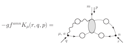
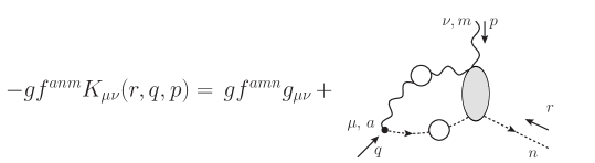
Figure E.1: The auxiliary functions $K_{\mu}(q,r,p)$ and $K_{\mu\nu}(q,r,p)$, appearing in the BQI of Eq. (E.1).

Now, using Eqs. (7.2) and (9.5), both $\widetilde{\rm{I}}\!\Gamma_{\mu}(r,p,q)$ and ${\rm{I}}\!\Gamma_{\mu}(r,p,q)$ introduce Schwinger poles of the form $q_{\mu}/q^{2}$ into Eq. (E.1). On the other hand, $K_{\mu}(r,q,p)$ has no external gluon legs, and hence no Schwinger poles, whereas $K_{\mu\nu}(r,q,p)$ can have poles at $p=0$, but not at $q=0$. Hence, equating residues of $1/q^{2}$ in Eq. (E.1) yields

$${\widetilde{C}}(r,p,q)=\left[1+G(q^{2})+L(q^{2})\right]C(r,p,q)\,.$$ (E.2)

Next, we expand Eq. (E.2) around $q=0$ and equate coefficients of equal orders to relate $C(r,-r,0)$ and ${\mathcal{C}}(r^{2})$ with their background counterparts. Specifically, using Eqs. (4.10), (7.22) and (9.9) and $L(0)=0$ [222], we obtain

$${\widetilde{C}}(r,-r,0)+2(q\cdot r){\widetilde{\mathcal{C}}}(r^{2})=F^{-1}(0)\left[C(r,-r,0)+2(q\cdot r){\mathcal{C}}(r^{2})\right]+{\cal O}(q^{2})\,.$$ (E.3)

Hence, equating zeroth order coefficients in Eq. (E.3) yields

$$C(r,-r,0)=F(0){\widetilde{C}}(r,-r,0)\,,$$ (E.4)

which combined with Eq. (9.8) implies Eq. (7.21).

Finally, the linear order terms lead to the result announced in the second line of Eq. (8.13).

In order to obtain the first line of Eq. (8.13), relating ${\mathbb{C}}(r^{2})$ to $\widetilde{\mathbb{C}}(r^{2})$, we use the BQI that converts between the $QQQ$ and $BQQ$ vertices, given by [111]

$$\widetilde{\rm{I}}\!\Gamma_{\alpha\mu\nu}(q,r,p)=\left\{\left[1+G(q^{2})\right]g^{\rho}_{\alpha}+L(q^{2})\frac{q_{\alpha}q^{\rho}}{q^{2}}\right\}{\rm{I}}\!\Gamma_{\rho\mu\nu}(q,r,p)+K_{\rho\nu\alpha}(r,q,p)P^{\rho}_{\mu}(r)\Delta^{-1}(r^{2})-K_{\rho\mu\alpha}(p,q,r)P^{\rho}_{\nu}(p)\Delta^{-1}(p^{2})\,,$$ (E.5)

where $K_{\rho\nu\alpha}(r,q,p)$ is the auxiliary function defined in Eq. (11.1).

While the vertices $\widetilde{\rm{I}}\!\Gamma_{\alpha\mu\nu}(q,r,p)$ and ${\rm{I}}\!\Gamma_{\alpha\mu\nu}(q,r,p)$ contain Schwinger poles in all channels [see Eq. (7.12)], only the simple poles at $q=0$ are relevant for deriving Eq. (8.13). Then, note that the auxiliary functions $K_{\rho\mu\alpha}(p,q,r)$ and $K_{\rho\nu\alpha}(r,q,p)$ can only contain Schwinger poles of the form $r_{\mu}/r^{2}$ and $p_{\nu}/p^{2}$, respectively. Hence, using Eqs. (7.1) and (7.12) and their background analogues, and isolating pole structures of the form $q_{\alpha}g_{\mu\nu}/q^{2}$ in Eq. (E.5), furnishes

$${\widetilde{V}}_{1}(q,r,p)=\left[1+G(q^{2})+L(q^{2})\right]V_{1}(q,r,p)\,.$$ (E.6)

At this point, we perform a Taylor expansion of Eq. (E.6) around $q=0$, to obtain

$${\widetilde{V}}_{1}(0,r,-r)+2(q\cdot r)\widetilde{\mathbb{C}}(r^{2})=F(0)\left[V_{1}(0,r,-r)+2(q\cdot r)\widetilde{\mathbb{C}}(r^{2})\right]+{\cal O}(q^{2})\,,$$ (E.7)

where we used again Eq. (4.10), $L(0)=0$, and the definitions of ${\mathbb{C}}(r^{2})$ and $\widetilde{\mathbb{C}}(r^{2})$ through Eq. (7.20) and its background equivalent.

Hence, equating zeroth order coefficients in Eq. (E.7), and using Eq. (7.19), we get

$${\widetilde{V}}_{1}(0,r,-r)=F^{-1}(0)V_{1}(0,r,-r)=0\,,$$ (E.8)

while the first-order terms lead to the first line in Eq. (8.13), which is the main result of this Appendix.

Appendix F Computing ${\cal W}(r^{2})$

An important component of the WI satisfied by the conventional three-gluon vertex, Eq. (12.4), is the function ${\cal W}(r^{2})$, originating from the ghost-gluon kernel. In this Appendix we derive the dynamical equation governing its momentum evolution [305, 146], and compute ${\cal W}(r^{2})$ numerically using lattice inputs [148].

To begin with, from Eq. (11.14) follows that ${\cal W}(r^{2})$ can be obtained from $K_{\mu\nu\alpha}(r,0,-r)$ through the projection

$${\cal W}(r^{2})=-\frac{1}{3}r^{\alpha}P^{\mu\nu}(r)K_{\mu\nu\alpha}(r,0,-r)=-\frac{1}{3}r^{\alpha}P^{\mu\nu}(r)\left[\frac{\partial H_{\mu\nu}(r,q,p)}{\partial q^{\alpha}}\right]_{q=0}\,,$$ (F.1)

where we use Eq. (11.13) to finally express ${\cal W}(r^{2})$ directly in terms of the ghost-gluon kernel.

Next, let us recall that $H_{\mu\nu}(r,q,p)$ is related to the ghost-gluon vertex, $\Gamma_{\nu}(r,q,p)$, through the STI [102]

$${\rm{I}}\!\Gamma_{\nu}(r,q,p)=r^{\mu}H_{\mu\nu}(r,q,p)\,.$$ (F.2)

Then, from Eqs. (F.1) and (F.2), we conclude that $H_{\nu\mu}(r,q,p)$ and ${\cal W}(r^{2})$ are renormalized by the same multiplicative constant, ${\widetilde{Z}}_{1}$, as $\Gamma_{\nu}(r,q,p)$, i.e.,

$${\cal W}_{{\scriptscriptstyle R}}(r^{2})={\widetilde{Z}}_{1}{\cal W}(r^{2})\,.$$ (F.3)

In particular, ${\cal W}(r^{2})$ is ultraviolet finite in the Landau gauge, and its renormalization amounts to a finite rescaling.

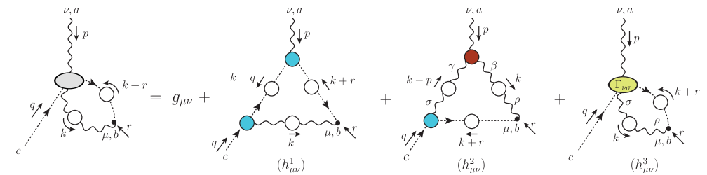
Figure F.1: SDE for the ghost-gluon scattering kernel, $H_{\mu\nu}(r,q,p)$.

Now, the ghost-gluon kernel satisfies the SDE given diagrammatically in Fig. F.1, where the yellow ellipse is the 1PI ghost-ghost-gluon-gluon vertex, $\Gamma_{\nu\sigma}$; at tree-level $\Gamma_{\nu\sigma}=0$. To date, $\Gamma_{\nu\sigma}$ has only been computed nonperturbatively in [280], where it was found that it has only a $\sim 2\%$ effect when inserted into the SDE of the ghost-gluon vertex, in the symmetric limit. In what follows, we will assume that the impact of $\Gamma_{\nu\sigma}$ in the behavior of ${\cal W}(r^{2})$ is also small, and will neglect diagram $h_{3}^{\nu\mu}$; see, however, the related discussion at the end of Sec. 22.

With this approximation, the dynamical equation determining ${\cal W}(r^{2})$ is given by

$${\cal W}(r^{2})={\cal W}_{1}(r^{2})+{\cal W}_{2}(r^{2})\,,$$ (F.4)

where the ${\cal W}_{i}(r^{2})$ are, respectively, the results of applying Eq. (F.1) to each of the diagrams $(h_{i}^{\mu\nu})$ of Fig. F.1, for $i=1,\,2$. After renormalization through Eqs. (2.35), (2.36) and (F.3), the ${\cal W}_{i}(r^{2})$ read

$${\cal W}_{1}(r^{2})= \,\frac{ig^{2}C_{\rm A}{\widetilde{Z}}_{1}}{6}\int_{k}\Delta(k^{2})D(k^{2})D(v^{2})(r\cdot k)f(k,r)B_{1}(v,-k,-r)B_{1}(k,0,-k)\,,$$

$${\cal W}_{2}(r^{2})= \,\frac{ig^{2}C_{\rm A}{\widetilde{Z}}_{1}}{6}\int_{k}\Delta(k^{2})\Delta(v^{2})D(v^{2})B_{1}(v,0,-v){\cal I}_{{\cal W}}(-r,-k,v)\,,$$ (F.5)

where $v:=k+r$, while $f(k,r)$ is given by

$$f(k,r)=1-\frac{(r\cdot k)^{2}}{r^{2}k^{2}}\,.$$ (F.6)

In Eq. (F.5) appear contributions from the dressed ghost-gluon and three-gluon vertices present in Fig. F.1. Specifically:

(i) $B_{1}(r,p,q)$ is the classical form factor of the ghost-gluon vertex, whose general tensor structure is given in Eq. (7.6); at tree-level $B_{1}^{(0)}=1$. Note that $B_{1}(r,p,q)$ can be obtained from ${\rm{I}}\!\Gamma_{\alpha}(r,p,q)$ through the transverse projection given by Eqs. (7.8) and (7.9) [with $C_{1}(r,p,q)=0$]; hence, it is free of Schwinger poles.

Moreover, $B_{1}(r,p,q)$ is a lattice observable in Landau gauge. However, for SU(3), $B_{1}(r,p,q)$ has so far only been evaluated on the lattice in the soft-gluon limit [11, 245, 246], while its general kinematics form is necessary for the calculation of ${\cal W}(r^{2})$. Thus, we determine $B_{1}(r,p,q)$ instead through its own SDE, truncated so as to preserve the STI of Eq. (F.2). The detailed analysis is presented in Sec. 8 of [99], and the result is shown on the right panel of Fig. 13 therein. We point out that in the soft-gluon limit this $B_{1}(r,p,q)$ reproduces the lattice data of [11, 245] (see Fig. 14 of [99]), and agrees qualitatively with various continuum studies [306, 307, 232, 167, 308, 215, 116, 269, 117].

(ii) The total contribution of the three-gluon vertex to the kernel of ${\cal W}(r^{2})$ is denoted by ${\cal I}_{{\cal W}}(q,r,p)$, and is given by the projection

$${\cal I}_{{\cal W}}(q,r,p):=\frac{1}{2}(q-r)^{\nu}\overline{\Gamma}^{\alpha}_{\alpha\nu}(q,r,p)\,,$$ (F.7)

where $\overline{\Gamma}_{\alpha\mu\nu}(q,r,p)$ is the transversely projected three-gluon vertex, defined in Eq. (22.5). Evidently, ${\cal I}_{{\cal W}}(q,r,p)$ is free of Schwinger poles.

In order to compute ${\cal I}_{{\cal W}}(q,r,p)$, we capitalize on the planar degeneracy property of the three-gluon gluon vertex [214, 213, 278, 116, 117, 190, 279, 251, 216, 99, 252]. Specifically, substituting Eq. (22.6) into Eq. (F.7) we obtain a compact and yet accurate expression for ${\cal I}_{{\cal W}}(q,r,p)$, namely

$${\cal I}_{{\cal W}}(q,r,p) \approx{\cal I}_{{\cal W}}^{0}(q,r,p)\mathit{L}_{{sg}}(s^{2})\,,\qquad s^{2}:=\frac{1}{2}(q^{2}+r^{2}+p^{2})\,,$$ (F.8)

where ${\cal I}_{{\cal W}}^{0}(q,r,p)$ is the tree-level value of ${\cal I}_{{\cal W}}$, given by

$${\cal I}_{{\cal W}}^{0}(q,r,p):=\frac{2f(q,r)}{p^{2}}\left[2q^{2}r^{2}-(q^{2}+r^{2})(q\cdot r)-(q\cdot r)^{2}\right]\,,$$ (F.9)

with $f(q,r)$ the function defined in Eq. (F.6). Note that Eq. (F.8) becomes exact in the limit $p=0$ [148].

Importantly, since ${\cal I}_{{\cal W}}(q,r,p)$ is a transverse projection it can be simulated directly on the lattice. This was done in general kinematics in [148], where it was shown that the error in Eq. (F.8) is less than $10\%$ for most of the kinematic region probed. Near the diagonal $q^{2}=r^{2}$, which is numerically the most important in the computation of ${\cal W}$ [146], this error falls below $1\%$ [148].

Then, using Eq. (F.8) for the ${\cal I}_{{\cal W}}$ in Eq. (F.5), the expression ${\cal W}_{2}(r^{2})$ reduces to

$${\cal W}_{2}(r^{2})=\frac{ig^{2}C_{\rm A}{\widetilde{Z}}_{1}}{3}\int_{k}\Delta(k^{2})\frac{\Delta(v^{2})D(v^{2})}{v^{2}}B_{1}(v,0,-v)f(k,r)\left[2r^{2}k^{2}-(r^{2}+k^{2})(r\cdot k)-(r\cdot k)^{2}\right]\mathit{L}_{{sg}}({\hat{s}}^{2})\,,$$ (F.10)

where we ${\hat{s}}^{2}=r^{2}+k^{2}+(r\cdot k)$.

For the numerical evaluation, we pass Eq. (F.4) to Euclidean space, using the rules and conventions of App. A, to obtain

$${\cal W}(x)={\cal W}_{1}(x)+{\cal W}_{2}(x)\,,$$ (F.11)

with the ${\cal W}_{i}(x)$ given by

$${\cal W}_{1}(x) =-\frac{\alpha_{s}C_{\rm A}{\widetilde{Z}}_{1}}{12\pi^{2}}\!\int_{0}^{\Lambda^{2}}\!\!dy\,y\sqrt{xy}\Delta(y)F(y)B_{1}(y,y,\pi)\int_{0}^{\pi}\!\!d\theta\,\frac{F(z)}{z}B_{1}(z,x,\chi)s_{\theta}^{4}c_{\theta}\,,$$

$${\cal W}_{2}(x) =-\frac{\alpha_{s}C_{\rm A}{\widetilde{Z}}_{1}}{6\pi^{2}}\!\int_{0}^{\Lambda^{2}}\!\!dy\,y^{2}\sqrt{xy}\Delta(y)\int_{0}^{\pi}\!\!d\theta\,\frac{\Delta(z)F(z)}{z^{2}}B_{1}(z,z,\pi)\mathit{L}_{{sg}}\left(x+y+\sqrt{xy}c_{\theta}\right)s_{\theta}^{4}\left[\sqrt{xy}(2+c_{\theta}^{2})-zc_{\theta}\right]\,,$$ (F.12)

where $z:=x+y+2\sqrt{xy}c_{\theta}$ and

$$\chi:=\cos^{-1}\left[-\frac{(\sqrt{x}+\sqrt{y}c_{\theta})}{\sqrt{z}}\right]\,.$$ (F.13)

At this point, we can evaluate Eq. (F.11) to obtain ${\cal W}(r^{2})$. We use the fits to lattice data of [23] for $\Delta(q^{2})$ and $F(q^{2})$, and of [190] for $\mathit{L}_{{sg}}(q^{2})$, shown previously in Fig. 12.1. All of these ingredients are renormalized in the asymmetric MOM scheme with $\mu=4.3$ GeV, for which the corresponding value of the coupling is $\alpha_{s}(4.3\text{ GeV})=0.27$ [189] and ${\widetilde{Z}}_{1}=0.933$ [148]. Finally, for $B_{1}$ we employ the general kinematics SDE result of [99].

With the above ingredients, we obtain for ${\cal W}(r^{2})$ the blue continuous curve on the left panel of Fig. 22.2. Propagating the statistical error of the lattice $\mathit{L}_{{sg}}(r^{2})$ to the ${\cal W}(r^{2})$ yields the error estimate shown as a blue band on the left panel of Fig. 22.2, whereas the effect of the errors of $\Delta(r^{2})$ and $F(q^{2})$ are negligible; for the details of this error analysis, see [148].

References

- [1] C.-N. Yang, R. L. Mills, Conservation of Isotopic Spin and Isotopic Gauge Invariance, Phys. Rev. 96 (1954) 191–195. doi:10.1103/PhysRev.96.191.
- [2] W. J. Marciano, H. Pagels, Quantum Chromodynamics: A Review, Phys. Rept. 36 (1978) 137. doi:10.1016/0370-1573(78)90208-9.
- [3] D. J. Gross, F. Wilczek, Ultraviolet Behavior of Nonabelian Gauge Theories, Phys. Rev. Lett. 30 (1973) 1343–1346. doi:10.1103/PhysRevLett.30.1343.
- [4] H. D. Politzer, Reliable Perturbative Results for Strong Interactions?, Phys. Rev. Lett. 30 (1973) 1346–1349. doi:10.1103/PhysRevLett.30.1346.
- [5] L. D. Faddeev, V. N. Popov, Feynman Diagrams for the Yang-Mills Field, Phys. Lett. B 25 (1967) 29–30. doi:10.1016/0370-2693(67)90067-6.
- [6] C. Becchi, A. Rouet, R. Stora, Renormalization of the Abelian Higgs-Kibble Model, Commun. Math. Phys. 42 (1975) 127–162. doi:10.1007/BF01614158.
- [7] C. Becchi, A. Rouet, R. Stora, Renormalization of Gauge Theories, Annals Phys. 98 (1976) 287–321. doi:10.1016/0003-4916(76)90156-1.
- [8] I. V. Tyutin, Gauge Invariance in Field Theory and Statistical Physics in Operator Formalism, LEBEDEV-75-39 (1975). arXiv:0812.0580.
- [9] G. ’t Hooft, M. J. G. Veltman, Regularization and Renormalization of Gauge Fields, Nucl. Phys. B 44 (1972) 189–213. doi:10.1016/0550-3213(72)90279-9.
- [10] C. G. Bollini, J. J. Giambiagi, Dimensional Renormalization: The Number of Dimensions as a Regularizing Parameter, Nuovo Cim. B 12 (1972) 20–26. doi:10.1007/BF02895558.
- [11] E.-M. Ilgenfritz, M. Muller-Preussker, A. Sternbeck, A. Schiller, I. Bogolubsky, Landau gauge gluon and ghost propagators from lattice QCD, Braz.J. Phys. 37 (2007) 193–200. arXiv:hep-lat/0609043, doi:10.1590/S0103-97332007000200006.
- [12] I. Bogolubsky, E. Ilgenfritz, M. Muller-Preussker, A. Sternbeck, The Landau gauge gluon and ghost propagators in 4D SU(3) gluodynamics in large lattice volumes, PoS LATTICE2007 (2007) 290. arXiv:0710.1968, doi:10.22323/1.042.0290.
- [13] I. Bogolubsky, E. Ilgenfritz, M. Muller-Preussker, A. Sternbeck, Lattice gluodynamics computation of Landau gauge Green’s functions in the deep infrared, Phys. Lett. B676 (2009) 69–73. arXiv:0901.0736, doi:10.1016/j.physletb.2009.04.076.
- [14] O. Oliveira, P. Silva, The Lattice infrared Landau gauge gluon propagator: The Infinite volume limit, PoS LAT2009 (2009) 226. arXiv:0910.2897, doi:10.22323/1.091.0226.
- [15] O. Oliveira, P. Bicudo, Running Gluon Mass from Landau Gauge Lattice QCD Propagator, J. Phys. G G38 (2011) 045003. arXiv:1002.4151, doi:10.1088/0954-3899/38/4/045003.
- [16] A. Ayala, A. Bashir, D. Binosi, M. Cristoforetti, J. Rodriguez-Quintero, Quark flavour effects on gluon and ghost propagators, Phys. Rev. D86 (2012) 074512. arXiv:1208.0795, doi:10.1103/PhysRevD.86.074512.
- [17] A. Sternbeck, M. Müller-Preussker, Lattice evidence for the family of decoupling solutions of Landau gauge Yang-Mills theory, Phys. Lett. B 726 (2013) 396–403. arXiv:1211.3057, doi:10.1016/j.physletb.2013.08.017.
- [18] P. Bicudo, D. Binosi, N. Cardoso, O. Oliveira, P. J. Silva, Lattice gluon propagator in renormalizable gauges, Phys. Rev. D92 (11) (2015) 114514. arXiv:1505.05897, doi:10.1103/PhysRevD.92.114514.
- [19] A. G. Duarte, O. Oliveira, P. J. Silva, Lattice Gluon and Ghost Propagators, and the Strong Coupling in Pure SU(3) Yang-Mills Theory: Finite Lattice Spacing and Volume Effects, Phys. Rev. D 94 (1) (2016) 014502. arXiv:1605.00594, doi:10.1103/PhysRevD.94.014502.
- [20] D. Binosi, C. D. Roberts, J. Rodriguez-Quintero, Scale-setting, flavor dependence, and chiral symmetry restoration, Phys. Rev. D 95 (11) (2017) 114009. arXiv:1611.03523, doi:10.1103/PhysRevD.95.114009.
- [21] D. Dudal, O. Oliveira, P. J. Silva, High precision statistical Landau gauge lattice gluon propagator computation vs. the Gribov–Zwanziger approach, Annals Phys. 397 (2018) 351–364. arXiv:1803.02281, doi:10.1016/j.aop.2018.08.019.
- [22] A. C. Aguilar, F. De Soto, M. N. Ferreira, J. Papavassiliou, J. Rodríguez-Quintero, S. Zafeiropoulos, Gluon propagator and three-gluon vertex with dynamical quarks, Eur. Phys. J. C80 (2) (2020) 154. arXiv:1912.12086, doi:10.1140/epjc/s10052-020-7741-0.
- [23] A. C. Aguilar, C. O. Ambrósio, F. De Soto, M. N. Ferreira, B. M. Oliveira, J. Papavassiliou, J. Rodríguez-Quintero, Ghost dynamics in the soft gluon limit, Phys. Rev. D 104 (5) (2021) 054028. arXiv:2107.00768, doi:10.1103/PhysRevD.104.054028.
- [24] A. Cucchieri, T. Mendes, What’s up with IR gluon and ghost propagators in Landau gauge? A puzzling answer from huge lattices, PoS LATTICE2007 (2007) 297. arXiv:0710.0412, doi:10.22323/1.042.0297.
- [25] A. Cucchieri, T. Mendes, Constraints on the IR behavior of the gluon propagator in Yang-Mills theories, Phys. Rev. Lett. 100 (2008) 241601. arXiv:0712.3517, doi:10.1103/PhysRevLett.100.241601.
- [26] A. Cucchieri, T. Mendes, E. M. S. Santos, Covariant gauge on the lattice: A New implementation, Phys. Rev. Lett. 103 (2009) 141602. arXiv:0907.4138, doi:10.1103/PhysRevLett.103.141602.
- [27] A. Cucchieri, T. Mendes, Numerical test of the Gribov-Zwanziger scenario in Landau gauge, PoS QCD-TNT09 (2009) 026. arXiv:1001.2584, doi:10.22323/1.087.0026.
- [28] A. Cucchieri, T. Mendes, Landau-gauge propagators in Yang-Mills theories at beta = 0: Massive solution versus conformal scaling, Phys. Rev. D81 (2010) 016005. arXiv:0904.4033, doi:10.1103/PhysRevD.81.016005.
- [29] A. Cucchieri, T. Mendes, G. M. Nakamura, E. M. S. Santos, Gluon Propagators in Linear Covariant Gauge, PoS FACESQCD (2010) 026. arXiv:1102.5233, doi:10.22323/1.117.0026.
- [30] G. Parisi, R. Petronzio, On Low-Energy Tests of QCD, Phys. Lett. B 94 (1980) 51–53. doi:10.1016/0370-2693(80)90822-9.
- [31] J. M. Cornwall, Dynamical Mass Generation in Continuum QCD, Phys. Rev. D 26 (1982) 1453. doi:10.1103/PhysRevD.26.1453.
- [32] C. W. Bernard, Monte Carlo Evaluation of the Effective Gluon Mass, Phys. Lett. B 108 (1982) 431–434. doi:10.1016/0370-2693(82)91228-X.
- [33] C. W. Bernard, Adjoint Wilson Lines and the Effective Gluon Mass, Nucl. Phys. B 219 (1983) 341–357. doi:10.1016/0550-3213(83)90645-4.
- [34] J. F. Donoghue, The Gluon ’Mass’ in the Bag Model, Phys. Rev. D 29 (1984) 2559. doi:10.1103/PhysRevD.29.2559.
- [35] J. Mandula, M. Ogilvie, The Gluon Is Massive: A Lattice Calculation of the Gluon Propagator in the Landau Gauge, Phys. Lett. B 185 (1987) 127–132. doi:10.1016/0370-2693(87)91541-3.
- [36] J. M. Cornwall, HOW d = 3 QCD RESEMBLES d = 4 QCD, Physica A 158 (1989) 97–110. doi:10.1016/0378-4371(89)90511-6.
- [37] J. M. Cornwall, J. Papavassiliou, Gauge Invariant Three Gluon Vertex in QCD, Phys. Rev. D 40 (1989) 3474. doi:10.1103/PhysRevD.40.3474.
- [38] M. Lavelle, Gauge invariant effective gluon mass from the operator product expansion, Phys. Rev. D 44 (1991) 26–28. doi:10.1103/PhysRevD.44.R26.
- [39] F. Halzen, G. I. Krein, A. A. Natale, Relating the QCD pomeron to an effective gluon mass, Phys. Rev. D 47 (1993) 295–298. doi:10.1103/PhysRevD.47.295.
- [40] K. G. Wilson, T. S. Walhout, A. Harindranath, W.-M. Zhang, R. J. Perry, S. D. Glazek, Nonperturbative QCD: A Weak coupling treatment on the light front, Phys. Rev. D49 (1994) 6720–6766. arXiv:hep-th/9401153, doi:10.1103/PhysRevD.49.6720.
- [41] A. Mihara, A. A. Natale, Dynamical gluon mass corrections in heavy quarkonia decays, Phys. Lett. B 482 (2000) 378–382. arXiv:hep-ph/0004236, doi:10.1016/S0370-2693(00)00546-3.
- [42] C. Alexandrou, P. de Forcrand, E. Follana, The Gluon propagator without lattice Gribov copies on a finer lattice, Phys. Rev. D 65 (2002) 114508. arXiv:hep-lat/0112043, doi:10.1103/PhysRevD.65.114508.
- [43] O. Philipsen, On the nonperturbative gluon mass and heavy quark physics, Nucl. Phys. B628 (2002) 167–192. arXiv:hep-lat/0112047, doi:10.1016/S0550-3213(02)00089-5.
- [44] A. C. Aguilar, A. A. Natale, P. S. Rodrigues da Silva, Relating a gluon mass scale to an infrared fixed point in pure gauge QCD, Phys. Rev. Lett. 90 (2003) 152001. arXiv:hep-ph/0212105, doi:10.1103/PhysRevLett.90.152001.
- [45] A. C. Aguilar, A. A. Natale, A Dynamical gluon mass solution in a coupled system of the Schwinger-Dyson equations, J. High Energy Phys. 08 (2004) 057. arXiv:hep-ph/0408254, doi:10.1088/1126-6708/2004/08/057.
- [46] A. C. Aguilar, J. Papavassiliou, Gluon mass generation in the PT-BFM scheme, J. High Energy Phys. 12 (2006) 012. arXiv:hep-ph/0610040, doi:10.1088/1126-6708/2006/12/012.
- [47] A. C. Aguilar, D. Binosi, J. Papavassiliou, Gluon and ghost propagators in the Landau gauge: Deriving lattice results from Schwinger-Dyson equations, Phys. Rev. D78 (2008) 025010. arXiv:0802.1870, doi:10.1103/PhysRevD.78.025010.
- [48] M. Tissier, N. Wschebor, Infrared propagators of Yang-Mills theory from perturbation theory, Phys. Rev. D 82 (2010) 101701. arXiv:1004.1607, doi:10.1103/PhysRevD.82.101701.
- [49] D. Binosi, D. Ibañez, J. Papavassiliou, The all-order equation of the effective gluon mass, Phys. Rev. D86 (2012) 085033. arXiv:1208.1451, doi:10.1103/PhysRevD.86.085033.
- [50] J. Serreau, M. Tissier, Lifting the Gribov ambiguity in Yang-Mills theories, Phys. Lett. B712 (2012) 97–103. arXiv:1202.3432, doi:10.1016/j.physletb.2012.04.041.
- [51] M. Peláez, M. Tissier, N. Wschebor, Two-point correlation functions of QCD in the Landau gauge, Phys. Rev. D 90 (2014) 065031. arXiv:1407.2005, doi:10.1103/PhysRevD.90.065031.
- [52] J. M. Cornwall, Exploring dynamical gluon mass generation in three dimensions, Phys. Rev. D 93 (2) (2016) 025021. arXiv:1510.03453, doi:10.1103/PhysRevD.93.025021.
- [53] F. Siringo, Analytical study of Yang–Mills theory in the infrared from first principles, Nucl. Phys. B907 (2016) 572–596. arXiv:1511.01015, doi:10.1016/j.nuclphysb.2016.04.028.
- [54] A. C. Aguilar, D. Binosi, C. T. Figueiredo, J. Papavassiliou, Unified description of seagull cancellations and infrared finiteness of gluon propagators, Phys. Rev. D94 (4) (2016) 045002. arXiv:1604.08456, doi:10.1103/PhysRevD.94.045002.
- [55] A. C. Aguilar, D. Binosi, J. Papavassiliou, Schwinger mechanism in linear covariant gauges, Phys. Rev. D95 (3) (2017) 034017. arXiv:1611.02096, doi:10.1103/PhysRevD.95.034017.
- [56] A. C. Aguilar, M. N. Ferreira, C. T. Figueiredo, J. Papavassiliou, Gluon mass scale through nonlinearities and vertex interplay, Phys. Rev. D 100 (9) (2019) 094039. arXiv:1909.09826, doi:10.1103/PhysRevD.100.094039.
- [57] J. Horak, F. Ihssen, J. Papavassiliou, J. M. Pawlowski, A. Weber, C. Wetterich, Gluon condensates and effective gluon mass, SciPost Phys. 13 (2) (2022) 042. arXiv:2201.09747, doi:10.21468/SciPostPhys.13.2.042.
- [58] C. J. Morningstar, M. J. Peardon, The Glueball spectrum from an anisotropic lattice study, Phys. Rev. D60 (1999) 034509. arXiv:hep-lat/9901004, doi:10.1103/PhysRevD.60.034509.
- [59] V. Mathieu, N. Kochelev, V. Vento, The Physics of Glueballs, Int. J. Mod. Phys. E18 (2009) 1–49. arXiv:0810.4453, doi:10.1142/S0218301309012124.
- [60] J. Meyers, E. S. Swanson, Spin Zero Glueballs in the Bethe-Salpeter Formalism, Phys. Rev. D87 (3) (2013) 036009. arXiv:1211.4648, doi:10.1103/PhysRevD.87.036009.
- [61] H. Sanchis-Alepuz, C. S. Fischer, C. Kellermann, L. von Smekal, Glueballs from the Bethe-Salpeter equation, Phys. Rev. D92 (2015) 034001. arXiv:1503.06051, doi:10.1103/PhysRevD.92.034001.
- [62] E. V. Souza, M. N. Ferreira, A. C. Aguilar, J. Papavassiliou, C. D. Roberts, S.-S. Xu, Pseudoscalar glueball mass: a window on three-gluon interactions, Eur. Phys. J. A 56 (1) (2020) 25. arXiv:1909.05875, doi:10.1140/epja/s10050-020-00041-y.
- [63] M. Q. Huber, C. S. Fischer, H. Sanchis-Alepuz, Spectrum of scalar and pseudoscalar glueballs from functional methods, Eur. Phys. J. C 80 (11) (2020) 1077. arXiv:2004.00415, doi:10.1140/epjc/s10052-020-08649-6.
- [64] A. Athenodorou, M. Teper, The glueball spectrum of SU(3) gauge theory in 3 + 1 dimensions, JHEP 11 (2020) 172. arXiv:2007.06422, doi:10.1007/JHEP11(2020)172.
- [65] A. Athenodorou, M. Teper, SU(N) gauge theories in 3+1 dimensions: glueball spectrum, string tensions and topology, JHEP 12 (2021) 082. arXiv:2106.00364, doi:10.1007/JHEP12(2021)082.
- [66] M. Q. Huber, C. S. Fischer, H. Sanchis-Alepuz, Higher spin glueballs from functional methods, Eur. Phys. J. C 81 (12) (2021) 1083, [Erratum: Eur.Phys.J.C 82, 38 (2022)]. arXiv:2110.09180, doi:10.1140/epjc/s10052-021-09864-5.
- [67] J. M. Pawlowski, C. S. Schneider, J. Turnwald, J. M. Urban, N. Wink, Yang-Mills glueball masses from spectral reconstruction, Phys. Rev. D 108 (7) (2023) 076018. arXiv:2212.01113, doi:10.1103/PhysRevD.108.076018.
- [68] M. Q. Huber, C. S. Fischer, H. Sanchis-Alepuz, Glueballs from Dyson-Schwinger and Bethe-Salpeter equations, Nuovo Cim. C 47 (4) (2024) 184. arXiv:2312.12029, doi:10.1393/ncc/i2024-24184-x.
- [69] J. C. Collins, A. Duncan, S. D. Joglekar, Trace and Dilatation Anomalies in Gauge Theories, Phys. Rev. D 16 (1977) 438–449. doi:10.1103/PhysRevD.16.438.
- [70] S. J. Brodsky, R. Shrock, Maximum Wavelength of Confined Quarks and Gluons and Properties of Quantum Chromodynamics, Phys. Lett. B666 (2008) 95–99. arXiv:0806.1535, doi:10.1016/j.physletb.2008.06.054.
- [71] D. Binosi, L. Chang, J. Papavassiliou, C. D. Roberts, Bridging a gap between continuum-QCD and ab initio predictions of hadron observables, Phys. Lett. B742 (2015) 183–188. arXiv:1412.4782, doi:10.1016/j.physletb.2015.01.031.
- [72] C. D. Roberts, S. M. Schmidt, Reflections upon the emergence of hadronic mass, Eur. Phys. J. ST 229 (22-23) (2020) 3319–3340. arXiv:2006.08782, doi:10.1140/epjst/e2020-000064-6.
- [73] C. D. Roberts, Empirical Consequences of Emergent Mass, Symmetry 12 (9) (2020) 1468. arXiv:2009.04011, doi:10.3390/sym12091468.
- [74] C. D. Roberts, On Mass and Matter, AAPPS Bull. 31 (2021) 6. arXiv:2101.08340, doi:10.1007/s43673-021-00005-4.
- [75] C. D. Roberts, D. G. Richards, T. Horn, L. Chang, Insights into the emergence of mass from studies of pion and kaon structure, Prog. Part. Nucl. Phys. 120 (2021) 103883. arXiv:2102.01765, doi:10.1016/j.ppnp.2021.103883.
- [76] D. Binosi, Emergent Hadron Mass in Strong Dynamics, Few Body Syst. 63 (2) (2022) 42. arXiv:2203.00942, doi:10.1007/s00601-022-01740-6.
- [77] J. Papavassiliou, Emergence of mass in the gauge sector of QCD*, Chin. Phys. C 46 (11) (2022) 112001. arXiv:2207.04977, doi:10.1088/1674-1137/ac84ca.
- [78] M. Ding, C. D. Roberts, S. M. Schmidt, Emergence of Hadron Mass and Structure, Particles 6 (2023) 57–120. arXiv:2211.07763, doi:10.3390/particles6010004.
- [79] C. D. Roberts, Origin of the Proton Mass, EPJ Web Conf. 282 (2023) 01006. arXiv:2211.09905, doi:10.1051/epjconf/202328201006.
- [80] G. ’t Hooft, On the Phase Transition Towards Permanent Quark Confinement, Nucl. Phys. B 138 (1978) 1–25. doi:10.1016/0550-3213(78)90153-0.
- [81] J. M. Cornwall, Quark Confinement and Vortices in Massive Gauge Invariant QCD, Nucl. Phys. B 157 (1979) 392–412. doi:10.1016/0550-3213(79)90111-1.
- [82] J. M. Cornwall, Center vortices and confinement versus screening, Phys. Rev. D 57 (1998) 7589–7600. arXiv:hep-th/9712248, doi:10.1103/PhysRevD.57.7589.
- [83] M. Engelhardt, K. Langfeld, H. Reinhardt, O. Tennert, Deconfinement in SU(2) Yang-Mills theory as a center vortex percolation transition, Phys. Rev. D 61 (2000) 054504. arXiv:hep-lat/9904004, doi:10.1103/PhysRevD.61.054504.
- [84] M. Engelhardt, H. Reinhardt, Center projection vortices in continuum Yang-Mills theory, Nucl. Phys. B 567 (2000) 249. arXiv:hep-th/9907139, doi:10.1016/S0550-3213(99)00727-0.
- [85] H. Reinhardt, Topology of center vortices, Nucl. Phys. B 628 (2002) 133–166. arXiv:hep-th/0112215, doi:10.1016/S0550-3213(02)00130-X.
- [86] J. Greensite, An introduction to the confinement problem, Vol. 821, Springer Berlin, Heidelberg, 2011. doi:10.1007/978-3-642-14382-3.
- [87] J. Braun, H. Gies, J. M. Pawlowski, Quark Confinement from Color Confinement, Phys. Lett. B684 (2010) 262–267. arXiv:0708.2413, doi:10.1016/j.physletb.2010.01.009.
- [88] L. Fister, J. M. Pawlowski, Confinement from Correlation Functions, Phys. Rev. D88 (2013) 045010. arXiv:1301.4163, doi:10.1103/PhysRevD.88.045010.
- [89] A. K. Cyrol, M. Mitter, J. M. Pawlowski, N. Strodthoff, Nonperturbative finite-temperature Yang-Mills theory, Phys. Rev. D 97 (5) (2018) 054015. arXiv:1708.03482, doi:10.1103/PhysRevD.97.054015.
- [90] J. S. Schwinger, Gauge Invariance and Mass, Phys. Rev. 125 (1962) 397–398. doi:10.1103/PhysRev.125.397.
- [91] J. S. Schwinger, Gauge Invariance and Mass. 2., Phys. Rev. 128 (1962) 2425–2429. doi:10.1103/PhysRev.128.2425.
- [92] E. Eichten, F. Feinberg, Dynamical Symmetry Breaking of Nonabelian Gauge Symmetries, Phys. Rev. D 10 (1974) 3254–3279. doi:10.1103/PhysRevD.10.3254.
- [93] J. Smit, On the Possibility That Massless Yang-Mills Fields Generate Massive Vector Particles, Phys. Rev. D 10 (1974) 2473. doi:10.1103/PhysRevD.10.2473.
- [94] A. C. Aguilar, J. Papavassiliou, On dynamical gluon mass generation, Eur.Phys.J. A31 (2007) 742–745. arXiv:0704.2308, doi:10.1140/epja/i2006-10281-7.
- [95] A. C. Aguilar, J. Papavassiliou, Gluon mass generation without seagull divergences, Phys. Rev. D81 (2010) 034003. arXiv:0910.4142, doi:10.1103/PhysRevD.81.034003.
- [96] A. C. Aguilar, D. Ibanez, V. Mathieu, J. Papavassiliou, Massless bound-state excitations and the Schwinger mechanism in QCD, Phys. Rev. D85 (2012) 014018. arXiv:1110.2633, doi:10.1103/PhysRevD.85.014018.
- [97] D. Ibañez, J. Papavassiliou, Gluon mass generation in the massless bound-state formalism, Phys. Rev. D87 (3) (2013) 034008. arXiv:1211.5314, doi:10.1103/PhysRevD.87.034008.
- [98] A. C. Aguilar, D. Binosi, J. Papavassiliou, The Gluon Mass Generation Mechanism: A Concise Primer, Front. Phys.(Beijing) 11 (2) (2016) 111203. arXiv:1511.08361, doi:10.1007/s11467-015-0517-6.
- [99] M. N. Ferreira, J. Papavassiliou, Gauge Sector Dynamics in QCD, Particles 6 (1) (2023) 312–363. arXiv:2301.02314, doi:10.3390/particles6010017.
- [100] M. N. Ferreira, J. Papavassiliou, Nonlinear Schwinger mechanism in QCD, and Fredholm alternatives theorem, Eur. Phys. J. C 84 (8) (2024) 835. arXiv:2407.04392, doi:10.1140/epjc/s10052-024-13223-5.
- [101] K. Fujikawa, B. W. Lee, A. I. Sanda, Generalized Renormalizable Gauge Formulation of Spontaneously Broken Gauge Theories, Phys. Rev. D 6 (1972) 2923–2943. doi:10.1103/PhysRevD.6.2923.
- [102] J. Taylor, Ward Identities and Charge Renormalization of the Yang-Mills Field, Nucl. Phys. B 33 (1971) 436–444. doi:10.1016/0550-3213(71)90297-5.
- [103] A. Slavnov, Ward Identities in Gauge Theories, Theor. Math. Phys. 10 (1972) 99–107. doi:10.1007/BF01090719.
- [104] F. J. Dyson, The S matrix in quantum electrodynamics, Phys. Rev. 75 (1949) 1736–1755. doi:10.1103/PhysRev.75.1736.
- [105] J. S. Schwinger, On the Green’s functions of quantized fields. 1., Proc. Nat. Acad. Sci. 37 (1951) 452–455. doi:10.1073/pnas.37.7.452.
- [106] C. D. Roberts, A. G. Williams, Dyson-Schwinger equations and their application to hadronic physics, Prog. Part. Nucl. Phys. 33 (1994) 477–575. arXiv:hep-ph/9403224, doi:10.1016/0146-6410(94)90049-3.
- [107] R. Alkofer, L. von Smekal, The Infrared behavior of QCD Green’s functions: Confinement dynamical symmetry breaking, and hadrons as relativistic bound states, Phys. Rept. 353 (2001) 281. arXiv:hep-ph/0007355, doi:10.1016/S0370-1573(01)00010-2.
- [108] C. S. Fischer, R. Alkofer, Nonperturbative propagators, running coupling and dynamical quark mass of Landau gauge QCD, Phys. Rev. D67 (2003) 094020. arXiv:hep-ph/0301094, doi:10.1103/PhysRevD.67.094020.
- [109] C. S. Fischer, Infrared properties of QCD from Dyson-Schwinger equations, J. Phys. G 32 (2006) R253–R291. arXiv:hep-ph/0605173, doi:10.1088/0954-3899/32/8/R02.
- [110] C. D. Roberts, Hadron Properties and Dyson-Schwinger Equations, Prog. Part. Nucl. Phys. 61 (2008) 50–65. arXiv:0712.0633, doi:10.1016/j.ppnp.2007.12.034.
- [111] D. Binosi, J. Papavassiliou, Pinch Technique: Theory and Applications, Phys. Rept. 479 (2009) 1–152. arXiv:0909.2536, doi:10.1016/j.physrep.2009.05.001.
- [112] A. Maas, Describing gauge bosons at zero and finite temperature, Phys. Rept. 524 (2013) 203–300. arXiv:1106.3942, doi:10.1016/j.physrep.2012.11.002.
- [113] A. Bashir, L. Chang, I. C. Cloet, B. El-Bennich, Y.-X. Liu, et al., Collective perspective on advances in Dyson-Schwinger Equation QCD, Commun. Theor. Phys. 58 (2012) 79–134. arXiv:1201.3366, doi:10.1088/0253-6102/58/1/16.
- [114] D. Binosi, L. Chang, J. Papavassiliou, S.-X. Qin, C. D. Roberts, Symmetry preserving truncations of the gap and Bethe-Salpeter equations, Phys. Rev. D93 (9) (2016) 096010. arXiv:1601.05441, doi:10.1103/PhysRevD.93.096010.
- [115] D. Binosi, C. Mezrag, J. Papavassiliou, C. D. Roberts, J. Rodriguez-Quintero, Process-independent strong running coupling, Phys. Rev. D96 (5) (2017) 054026. arXiv:1612.04835, doi:10.1103/PhysRevD.96.054026.
- [116] M. Q. Huber, Nonperturbative properties of Yang-Mills theories, Phys. Rept. 879 (2020) 1–92. arXiv:1808.05227, doi:10.1016/j.physrep.2020.04.004.
- [117] M. Q. Huber, Correlation functions of Landau gauge Yang-Mills theory, Phys. Rev. D 101 (2020) 114009. arXiv:2003.13703, doi:10.1103/PhysRevD.101.114009.
- [118] D. Binosi, J. Papavassiliou, Gauge-invariant truncation scheme for the Schwinger-Dyson equations of QCD, Phys. Rev. D77 (2008) 061702. arXiv:0712.2707, doi:10.1103/PhysRevD.77.061702.
- [119] A. Pilaftsis, Generalized pinch technique and the background field method in general gauges, Nucl. Phys. B 487 (1997) 467–491. arXiv:hep-ph/9607451, doi:10.1016/S0550-3213(96)00686-4.
- [120] D. Binosi, J. Papavassiliou, The Pinch technique to all orders, Phys. Rev. D 66 (2002) 111901. arXiv:hep-ph/0208189, doi:10.1103/PhysRevD.66.111901.
- [121] D. Binosi, J. Papavassiliou, Pinch technique selfenergies and vertices to all orders in perturbation theory, J. Phys. G G30 (2004) 203. arXiv:hep-ph/0301096, doi:10.1088/0954-3899/30/2/017.
- [122] J. M. Cornwall, J. Papavassiliou, D. Binosi, The Pinch Technique and its Applications to Non-Abelian Gauge Theories, Cambridge University Press, 2011. doi:10.1017/9781009402415.
- [123] B. S. DeWitt, Quantum Theory of Gravity. 2. The Manifestly Covariant Theory, Phys. Rev. 162 (1967) 1195–1239. doi:10.1103/PhysRev.162.1195.
- [124] G. ’t Hooft, Renormalizable Lagrangians for Massive Yang-Mills Fields, Nucl. Phys. B 35 (1971) 167–188. doi:10.1016/0550-3213(71)90139-8.
- [125] J. Honerkamp, The Question of invariant renormalizability of the massless Yang-Mills theory in a manifest covariant approach, Nucl. Phys. B 48 (1972) 269–287. doi:10.1016/0550-3213(72)90063-6.
- [126] R. E. Kallosh, The Renormalization in Nonabelian Gauge Theories, Nucl. Phys. B 78 (1974) 293–312. doi:10.1016/0550-3213(74)90284-3.
- [127] I. Y. Arefeva, L. D. Faddeev, A. A. Slavnov, Generating Functional for the s Matrix in Gauge Theories, Teor. Mat. Fiz. 21 (1974) 311–321. doi:10.1007/BF01038094.
- [128] H. Kluberg-Stern, J. B. Zuber, Renormalization of Nonabelian Gauge Theories in a Background Field Gauge. 1. Green Functions, Phys. Rev. D 12 (1975) 482–488. doi:10.1103/PhysRevD.12.482.
- [129] S. Weinberg, Effective Gauge Theories, Phys. Lett. B 91 (1980) 51–55. doi:10.1016/0370-2693(80)90660-7.
- [130] L. Abbott, The Background Field Method Beyond One Loop, Nucl. Phys. B 185 (1981) 189–203. doi:10.1016/0550-3213(81)90371-0.
- [131] G. M. Shore, Symmetry Restoration and the Background Field Method in Gauge Theories, Annals Phys. 137 (1981) 262. doi:10.1016/0003-4916(81)90198-6.
- [132] L. F. Abbott, Introduction to the Background Field Method, Acta Phys. Polon. B 13 (1982) 33.
- [133] L. F. Abbott, M. T. Grisaru, R. K. Schaefer, The Background Field Method and the S Matrix, Nucl. Phys. B 229 (1983) 372–380. doi:10.1016/0550-3213(83)90337-1.
- [134] D. Binosi, J. Papavassiliou, New Schwinger-Dyson equations for non-Abelian gauge theories, J. High Energy Phys. 11 (2008) 063. arXiv:0805.3994, doi:10.1088/1126-6708/2008/11/063.
- [135] A. C. Aguilar, M. N. Ferreira, D. Ibañez, B. M. Oliveira, J. Papavassiliou, Patterns of gauge symmetry in the background field method, Eur. Phys. J. C 83 (1) (2023) 86. arXiv:2211.16102, doi:10.1140/epjc/s10052-023-11219-1.
- [136] A. C. Aguilar, M. N. Ferreira, B. M. Oliveira, J. Papavassiliou, Schwinger–Dyson truncations in the all-soft limit: a case study, Eur. Phys. J. C 82 (11) (2022) 1068. arXiv:2210.07429, doi:10.1140/epjc/s10052-022-11034-0.
- [137] P. A. Grassi, T. Hurth, M. Steinhauser, Practical algebraic renormalization, Annals Phys. 288 (2001) 197–248. arXiv:hep-ph/9907426, doi:10.1006/aphy.2001.6117.
- [138] P. A. Grassi, T. Hurth, M. Steinhauser, The Algebraic method, Nucl. Phys. B 610 (2001) 215–250. arXiv:hep-ph/0102005, doi:10.1016/S0550-3213(01)00303-0.
- [139] D. Binosi, J. Papavassiliou, Pinch technique and the Batalin-Vilkovisky formalism, Phys. Rev. D66 (2002) 025024. arXiv:hep-ph/0204128, doi:10.1103/PhysRevD.66.025024.
- [140] D. Binosi, A. Quadri, AntiBRST symmetry and Background Field Method, Phys. Rev. D88 (2013) 085036. arXiv:1309.1021, doi:10.1103/PhysRevD.88.085036.
- [141] J. C. Collins, Renormalization : An Introduction to Renormalization, the Renormalization Group and the Operator-Product Expansion, Vol. 26 of Cambridge Monographs on Mathematical Physics, Cambridge University Press, Cambridge, 1984. doi:10.1017/9781009401807.
- [142] E. C. Poggio, E. Tomboulis, S. H. H. Tye, Dynamical Symmetry Breaking in Nonabelian Field Theories, Phys. Rev. D11 (1975) 2839. doi:10.1103/PhysRevD.11.2839.
- [143] N. Alkofer, R. Alkofer, Features of ghost-gluon and ghost-quark bound states related to BRST quartets, Phys. Lett. B 702 (2011) 158–163. arXiv:1102.2753, doi:10.1016/j.physletb.2011.06.073.
- [144] A. C. Aguilar, D. Binosi, C. T. Figueiredo, J. Papavassiliou, Evidence of ghost suppression in gluon mass scale dynamics, Eur. Phys. J. C78 (3) (2018) 181. arXiv:1712.06926, doi:10.1140/epjc/s10052-018-5679-2.
- [145] G. Eichmann, J. M. Pawlowski, J. a. M. Silva, Mass generation in Landau-gauge Yang-Mills theory, Phys. Rev. D 104 (11) (2021) 114016. arXiv:2107.05352, doi:10.1103/PhysRevD.104.114016.
- [146] A. C. Aguilar, M. N. Ferreira, J. Papavassiliou, Exploring smoking-gun signals of the Schwinger mechanism in QCD, Phys. Rev. D 105 (1) (2022) 014030. arXiv:2111.09431, doi:10.1103/PhysRevD.105.014030.
- [147] D. Binosi, J. Papavassiliou, Coupled dynamics in gluon mass generation and the impact of the three-gluon vertex, Phys. Rev. D97 (5) (2018) 054029. arXiv:1709.09964, doi:10.1103/PhysRevD.97.054029.
- [148] A. C. Aguilar, F. De Soto, M. N. Ferreira, J. Papavassiliou, F. Pinto-Gómez, C. D. Roberts, J. Rodríguez-Quintero, Schwinger mechanism for gluons from lattice QCD, Phys. Lett. B 841 (2023) 137906. arXiv:2211.12594, doi:10.1016/j.physletb.2023.137906.
- [149] A. C. Aguilar, M. N. Ferreira, B. M. Oliveira, J. Papavassiliou, L. R. Santos, Schwinger poles of the three-gluon vertex: symmetry and dynamics, Eur. Phys. J. C 83 (10) (2023) 889. arXiv:2306.16283, doi:10.1140/epjc/s10052-023-12058-w.
- [150] V. Vladimirov, Equations of Mathematical Physics, Monographs and textbooks in pure and applied mathematics, M. Dekker, 1971.
- [151] A. Polyanin, A. Manzhirov, Handbook of Integral Equations: Second Edition, Taylor & Francis, 2008. doi:10.1201/9781420010558.
- [152] K.-I. Kondo, Vacuum condensate of mass dimension 2 as the origin of mass gap and quark confinement, Phys. Lett. B 514 (2001) 335–345. arXiv:hep-th/0105299, doi:10.1016/S0370-2693(01)00817-6.
- [153] D. Epple, H. Reinhardt, W. Schleifenbaum, A. P. Szczepaniak, Subcritical solution of the Yang-Mills Schroedinger equation in the Coulomb gauge, Phys. Rev. D77 (2008) 085007. arXiv:0712.3694, doi:10.1103/PhysRevD.77.085007.
- [154] D. Dudal, J. A. Gracey, S. P. Sorella, N. Vandersickel, H. Verschelde, A refinement of the Gribov-Zwanziger approach in the Landau gauge: infrared propagators in harmony with the lattice results, Phys. Rev. D78 (2008) 065047. arXiv:0806.4348, doi:10.1103/PhysRevD.78.065047.
- [155] C. S. Fischer, A. Maas, J. M. Pawlowski, On the infrared behavior of Landau gauge Yang-Mills theory, Annals Phys. 324 (2009) 2408–2437. arXiv:0810.1987, doi:10.1016/j.aop.2009.07.009.
- [156] K.-I. Kondo, Infrared behavior of the ghost propagator in the Landau gauge Yang-Mills theory, Prog. Theor. Phys. 122 (2010) 1455–1475. arXiv:0907.3249, doi:10.1143/PTP.122.1455.
- [157] M. Q. Huber, R. Alkofer, S. P. Sorella, Infrared analysis of Dyson-Schwinger equations taking into account the Gribov horizon in Landau gauge, Phys. Rev. D 81 (2010) 065003. arXiv:0910.5604, doi:10.1103/PhysRevD.81.065003.
- [158] J. A. Gracey, Alternative refined Gribov-Zwanziger Lagrangian, Phys. Rev. D 82 (2010) 085032. arXiv:1009.3889, doi:10.1103/PhysRevD.82.085032.
- [159] D. R. Campagnari, H. Reinhardt, Non-Gaussian wave functionals in Coulomb gauge Yang–Mills theory, Phys. Rev. D82 (2010) 105021. arXiv:1009.4599, doi:10.1103/PhysRevD.82.105021.
- [160] M. Tissier, N. Wschebor, An Infrared Safe perturbative approach to Yang-Mills correlators, Phys. Rev. D84 (2011) 045018. arXiv:1105.2475, doi:10.1103/PhysRevD.84.045018.
- [161] D. A. Fagundes, E. G. S. Luna, M. J. Menon, A. A. Natale, Aspects of a Dynamical Gluon Mass Approach to Elastic Hadron Scattering at LHC, Nucl. Phys. A 886 (2012) 48–70. arXiv:1112.4680, doi:10.1016/j.nuclphysa.2012.05.002.
- [162] N. Vandersickel, D. Zwanziger, The Gribov problem and QCD dynamics, Phys. Rept. 520 (2012) 175–251. arXiv:1202.1491, doi:10.1016/j.physrep.2012.07.003.
- [163] M. A. L. Capri, D. Dudal, M. S. Guimaraes, L. F. Palhares, S. P. Sorella, An all-order proof of the equivalence between Gribov’s no-pole and Zwanziger’s horizon conditions, Phys. Lett. B 719 (2013) 448–453. arXiv:1212.2419, doi:10.1016/j.physletb.2013.01.039.
- [164] M. Pelaez, M. Tissier, N. Wschebor, Three-point correlation functions in Yang-Mills theory, Phys. Rev. D88 (2013) 125003. arXiv:1310.2594, doi:10.1103/PhysRevD.88.125003.
- [165] F. Siringo, Gluon propagator in Feynman gauge by the method of stationary variance, Phys. Rev. D 90 (9) (2014) 094021. arXiv:1408.5313, doi:10.1103/PhysRevD.90.094021.
- [166] M. A. L. Capri, D. Dudal, D. Fiorentini, M. S. Guimaraes, I. F. Justo, A. D. Pereira, B. W. Mintz, L. F. Palhares, R. F. Sobreiro, S. P. Sorella, Exact nilpotent nonperturbative BRST symmetry for the Gribov-Zwanziger action in the linear covariant gauge, Phys. Rev. D 92 (4) (2015) 045039. arXiv:1506.06995, doi:10.1103/PhysRevD.92.045039.
- [167] A. K. Cyrol, L. Fister, M. Mitter, J. M. Pawlowski, N. Strodthoff, Landau gauge Yang-Mills correlation functions, Phys. Rev. D94 (5) (2016) 054005. arXiv:1605.01856, doi:10.1103/PhysRevD.94.054005.
- [168] S. D. Glazek, M. Gómez-Rocha, J. More, K. Serafin, Renormalized quark–antiquark Hamiltonian induced by a gluon mass ansatz in heavy-flavor QCD, Phys. Lett. B773 (2017) 172–178. arXiv:1705.07629, doi:10.1016/j.physletb.2017.08.018.
- [169] J. A. Gracey, M. Peláez, U. Reinosa, M. Tissier, Two loop calculation of Yang-Mills propagators in the Curci-Ferrari model, Phys. Rev. D 100 (3) (2019) 034023. arXiv:1905.07262, doi:10.1103/PhysRevD.100.034023.
- [170] A. C. Aguilar, M. . N. Ferreira, D. Ibañez, J. Papavassiliou, Schwinger displacement of the quark–gluon vertex, Eur. Phys. J. C 83 (10) (2023) 967. arXiv:2308.16297, doi:10.1140/epjc/s10052-023-12103-8.
- [171] C. Itzykson, J. B. Zuber, Quantum Field Theory, International Series In Pure and Applied Physics, McGraw-Hill, New York, 1980.
- [172] P. Pascual, R. Tarrach, QCD: Renormalization for the Practitioner, Vol. 194, Springer Berlin, Heidelberg, 1984. doi:10.1007/3-540-12908-1.
- [173] R. J. Rivers, PATH INTEGRAL METHODS IN QUANTUM FIELD THEORY, Cambridge Monographs on Mathematical Physics, Cambridge University Press, 1988. doi:10.1017/CBO9780511564055.
- [174] D. Binosi, D. Ibañez, J. Papavassiliou, Nonperturbative study of the four gluon vertex, J. High Energy Phys. 09 (2014) 059. arXiv:1407.3677, doi:10.1007/JHEP09(2014)059.
- [175] J. C. Ward, An Identity in Quantum Electrodynamics, Phys. Rev. 78 (1950) 182. doi:10.1103/PhysRev.78.182.
- [176] Y. Takahashi, On the generalized Ward identity, Nuovo Cim. 6 (1957) 371. doi:10.1007/BF02832514.
- [177] J. S. Ball, T.-W. Chiu, Analytic Properties of the Vertex Function in Gauge Theories. 2., Phys. Rev. D 22 (1980) 2550, [Erratum: Phys. Rev. D 23, 3085 (1981)]. doi:10.1103/PhysRevD.22.2550.
- [178] A. I. Davydychev, P. Osland, O. Tarasov, Three gluon vertex in arbitrary gauge and dimension, Phys. Rev. D 54 (1996) 4087–4113, [Erratum: Phys. Rev. D 59, 109901 (1999)]. arXiv:hep-ph/9605348, doi:10.1103/PhysRevD.59.109901.
- [179] L. von Smekal, A. Hauck, R. Alkofer, A Solution to Coupled Dyson–Schwinger Equations for Gluons and Ghosts in Landau Gauge, Annals Phys. 267 (1998) 1–60, [Erratum: Annals Phys. 269, 182 (1998)]. arXiv:hep-ph/9707327, doi:10.1006/aphy.1998.5806,10.1006/aphy.1998.5864.
- [180] D. Binosi, J. Papavassiliou, Gauge invariant Ansatz for a special three-gluon vertex, J. High Energy Phys. 03 (2011) 121. arXiv:1102.5662, doi:10.1007/JHEP03(2011)121.
- [181] J. Gracey, H. Kißler, D. Kreimer, Self-consistency of off-shell Slavnov-Taylor identities in QCD, Phys. Rev. D 100 (8) (2019) 085001. arXiv:1906.07996, doi:10.1103/PhysRevD.100.085001.
- [182] A. C. Aguilar, M. N. Ferreira, J. Papavassiliou, Novel sum rules for the three-point sector of QCD, Eur. Phys. J. C 80 (9) (2020) 887. arXiv:2006.04587, doi:10.1140/epjc/s10052-020-08453-2.
- [183] W. Celmaster, R. J. Gonsalves, The Renormalization Prescription Dependence of the QCD Coupling Constant, Phys. Rev. D 20 (1979) 1420. doi:10.1103/PhysRevD.20.1420.
- [184] A. Hasenfratz, P. Hasenfratz, The Connection Between the Lambda Parameters of Lattice and Continuum QCD, Phys. Lett. B 93 (1980) 165. doi:10.1016/0370-2693(80)90118-5.
- [185] E. Braaten, J. P. Leveille, Minimal Subtraction and Momentum Subtraction in QCD at Two Loop Order, Phys. Rev. D 24 (1981) 1369. doi:10.1103/PhysRevD.24.1369.
- [186] P. Boucaud, J. P. Leroy, J. Micheli, O. Pene, C. Roiesnel, Three loop beta function and nonperturbative alpha(s) in asymmetric momentum scheme, JHEP 12 (1998) 004. arXiv:hep-ph/9810437, doi:10.1088/1126-6708/1998/12/004.
- [187] K. G. Chetyrkin, A. Retey, Three loop three linear vertices and four loop similar to MOM beta functions in massless QCD (7 2000). arXiv:hep-ph/0007088.
- [188] A. Athenodorou, D. Binosi, P. Boucaud, F. De Soto, J. Papavassiliou, J. Rodriguez-Quintero, S. Zafeiropoulos, On the zero crossing of the three-gluon vertex, Phys. Lett. B761 (2016) 444–449. arXiv:1607.01278, doi:10.1016/j.physletb.2016.08.065.
- [189] P. Boucaud, F. De Soto, J. Rodríguez-Quintero, S. Zafeiropoulos, Refining the detection of the zero crossing for the three-gluon vertex in symmetric and asymmetric momentum subtraction schemes, Phys. Rev. D95 (11) (2017) 114503. arXiv:1701.07390, doi:10.1103/PhysRevD.95.114503.
- [190] A. C. Aguilar, F. De Soto, M. N. Ferreira, J. Papavassiliou, J. Rodríguez-Quintero, Infrared facets of the three-gluon vertex, Phys. Lett. B 818 (2021) 136352. arXiv:2102.04959, doi:10.1016/j.physletb.2021.136352.
- [191] P. Ramond, Field theory: a modern primer, Vol. 51 of Frontiers in Physics: A Lecture Note and Reprint Series, Benjamin/Cummings Publishing Company, Advanced Book Program, 1981.
- [192] R. Alkofer, M. Q. Huber, K. Schwenzer, Algorithmic derivation of Dyson-Schwinger Equations, Comput. Phys. Commun. 180 (2009) 965–976. arXiv:0808.2939, doi:10.1016/j.cpc.2008.12.009.
- [193] E. S. Swanson, A Primer on Functional Methods and the Schwinger-Dyson Equations, AIP Conf. Proc. 1296 (1) (2010) 75–121. arXiv:1008.4337, doi:10.1063/1.3523221.
- [194] J. M. Pawlowski, D. F. Litim, S. Nedelko, L. von Smekal, Infrared behavior and fixed points in Landau gauge QCD, Phys. Rev. Lett. 93 (2004) 152002. arXiv:hep-th/0312324, doi:10.1103/PhysRevLett.93.152002.
- [195] J. M. Pawlowski, Aspects of the functional renormalisation group, Annals Phys. 322 (2007) 2831–2915. arXiv:hep-th/0512261, doi:10.1016/j.aop.2007.01.007.
- [196] M. E. Carrington, Renormalization group flow equations connected to the -particle-irreducible effective action, Phys. Rev. D87 (4) (2013) 045011. arXiv:1211.4127, doi:10.1103/PhysRevD.87.045011.
- [197] M. E. Carrington, W.-J. Fu, D. Pickering, J. W. Pulver, Renormalization group methods and the 2PI effective action, Phys. Rev. D 91 (2) (2015) 025003. arXiv:1404.0710, doi:10.1103/PhysRevD.91.025003.
- [198] A. K. Cyrol, M. Mitter, J. M. Pawlowski, N. Strodthoff, Nonperturbative quark, gluon, and meson correlators of unquenched QCD, Phys. Rev. D97 (5) (2018) 054006. arXiv:1706.06326, doi:10.1103/PhysRevD.97.054006.
- [199] L. Corell, A. K. Cyrol, M. Mitter, J. M. Pawlowski, N. Strodthoff, Correlation functions of three-dimensional Yang-Mills theory from the FRG, SciPost Phys. 5 (6) (2018) 066. arXiv:1803.10092, doi:10.21468/SciPostPhys.5.6.066.
- [200] N. Dupuis, L. Canet, A. Eichhorn, W. Metzner, J. M. Pawlowski, M. Tissier, N. Wschebor, The nonperturbative functional renormalization group and its applications, Phys. Rept. 910 (2021) 1–114. arXiv:2006.04853, doi:10.1016/j.physrep.2021.01.001.
- [201] J.-P. Blaizot, J. M. Pawlowski, U. Reinosa, Functional renormalization group and 2PI effective action formalism, Annals Phys. 431 (2021) 168549. arXiv:2102.13628, doi:10.1016/j.aop.2021.168549.
- [202] J. M. Cornwall, R. Jackiw, E. Tomboulis, Effective Action for Composite Operators, Phys. Rev. D 10 (1974) 2428–2445. doi:10.1103/PhysRevD.10.2428.
- [203] J. Cornwall, R. Norton, Spontaneous Symmetry Breaking Without Scalar Mesons, Phys. Rev. D 8 (1973) 3338–3346. doi:10.1103/PhysRevD.8.3338.
- [204] J. Berges, N-particle irreducible effective action techniques for gauge theories, Phys. Rev. D 70 (2004) 105010. arXiv:hep-ph/0401172, doi:10.1103/PhysRevD.70.105010.
- [205] J. Berges, Introduction to nonequilibrium quantum field theory, AIP Conf. Proc. 739 (1) (2004) 3–62. arXiv:hep-ph/0409233, doi:10.1063/1.1843591.
- [206] J. Berges, S. Borsanyi, U. Reinosa, J. Serreau, Nonperturbative renormalization for 2PI effective action techniques, Annals Phys. 320 (2005) 344–398. arXiv:hep-ph/0503240, doi:10.1016/j.aop.2005.06.001.
- [207] R. Alkofer, C. S. Fischer, F. J. Llanes-Estrada, K. Schwenzer, The Quark-gluon vertex in Landau gauge QCD: Its role in dynamical chiral symmetry breaking and quark confinement, Annals Phys. 324 (2009) 106–172. arXiv:0804.3042, doi:10.1016/j.aop.2008.07.001.
- [208] M. E. Carrington, Y. Guo, Techniques for n-Particle Irreducible Effective Theories, Phys. Rev. D 83 (2011) 016006. arXiv:1010.2978, doi:10.1103/PhysRevD.83.016006.
- [209] M. C. A. York, G. D. Moore, M. Tassler, 3-loop 3PI effective action for 3D SU(3) QCD, JHEP 06 (2012) 077. arXiv:1202.4756, doi:10.1007/JHEP06(2012)077.
- [210] M. E. Carrington, W. Fu, T. Fugleberg, D. Pickering, I. Russell, Bethe-Salpeter Equations from the 4PI effective action, Phys. Rev. D 88 (2013) 085024. arXiv:1310.3295, doi:10.1103/PhysRevD.88.085024.
- [211] R. Williams, C. S. Fischer, W. Heupel, Light mesons in QCD and unquenching effects from the 3PI effective action, Phys. Rev. D93 (3) (2016) 034026. arXiv:1512.00455, doi:10.1103/PhysRevD.93.034026.
- [212] A. K. Cyrol, M. Q. Huber, L. von Smekal, A Dyson–Schwinger study of the four-gluon vertex, Eur. Phys. J. C75 (2015) 102. arXiv:1408.5409, doi:10.1140/epjc/s10052-015-3312-1.
- [213] A. Blum, M. Q. Huber, M. Mitter, L. von Smekal, Gluonic three-point correlations in pure Landau gauge QCD, Phys. Rev. D89 (2014) 061703. arXiv:1401.0713, doi:10.1103/PhysRevD.89.061703.
- [214] G. Eichmann, R. Williams, R. Alkofer, M. Vujinovic, The three-gluon vertex in Landau gauge, Phys. Rev. D89 (2014) 105014. arXiv:1402.1365, doi:10.1103/PhysRevD.89.105014.
- [215] A. C. Aguilar, M. N. Ferreira, C. T. Figueiredo, J. Papavassiliou, Nonperturbative structure of the ghost-gluon kernel, Phys. Rev. D99 (2019) 034026. arXiv:1811.08961, doi:10.1103/PhysRevD.99.034026.
- [216] A. C. Aguilar, M. N. Ferreira, J. Papavassiliou, L. R. Santos, Planar degeneracy of the three-gluon vertex, Eur. Phys. J. C 83 (6) (2023) 549. arXiv:2305.05704, doi:10.1140/epjc/s10052-023-11732-3.
- [217] A. C. Aguilar, M. N. Ferreira, J. Papavassiliou, L. R. Santos, Four-gluon vertex in collinear kinematics, Eur. Phys. J. C 84 (7) (2024) 676. arXiv:2402.16071, doi:10.1140/epjc/s10052-024-12970-9.
- [218] A. C. Aguilar, F. De Soto, M. N. Ferreira, J. Papavassiliou, F. Pinto-Gómez, J. Rodríguez-Quintero, L. R. Santos, Nonperturbative four-gluon vertex in soft kinematics, Phys. Lett. B 858 (2024) 139065. arXiv:2408.06135, doi:10.1016/j.physletb.2024.139065.
- [219] A. C. Aguilar, M. N. Ferreira, B. M. Oliveira, J. Papavassiliou, G. T. Linhares, Infrared properties of the quark-gluon vertex in general kinematics, Eur. Phys. J. C 84 (11) (2024) 1231. arXiv:2408.15370, doi:10.1140/epjc/s10052-024-13605-9.
- [220] P. A. Grassi, T. Hurth, A. Quadri, On the Landau background gauge fixing and the IR properties of YM Green functions, Phys. Rev. D 70 (2004) 105014. arXiv:hep-th/0405104, doi:10.1103/PhysRevD.70.105014.
- [221] A. C. Aguilar, N. Brito, M. N. Ferreira, J. Papavassiliou, O. Oliveira, P. J. Silva, Lattice determination of the Batalin-Vilkovisky function and the strong running interaction, Phys. Lett. B 858 (2024) 139054. arXiv:2404.06496, doi:10.1016/j.physletb.2024.139054.
- [222] A. C. Aguilar, D. Binosi, J. Papavassiliou, J. Rodriguez-Quintero, Non-perturbative comparison of QCD effective charges, Phys. Rev. D80 (2009) 085018. arXiv:0906.2633, doi:10.1103/PhysRevD.80.085018.
- [223] T. Kugo, The Universal renormalization factors Z(1) / Z(3) and color confinement condition in nonAbelian gauge theory, in: International Symposium on BRS Symmetry on the Occasion of Its 20th Anniversary, 1995, pp. 107–119. arXiv:hep-th/9511033.
- [224] K.-I. Kondo, Kugo-Ojima color confinement criterion and Gribov-Zwanziger horizon condition, Phys. Lett. B 678 (2009) 322–330. arXiv:0904.4897, doi:10.1016/j.physletb.2009.06.026.
- [225] A. C. Aguilar, D. Binosi, J. Papavassiliou, Indirect determination of the Kugo-Ojima function from lattice data, J. High Energy Phys. 11 (2009) 066. arXiv:0907.0153, doi:10.1088/1126-6708/2009/11/066.
- [226] A. Cucchieri, T. Mendes, Constraints on the IR behavior of the ghost propagator in Yang-Mills theories, Phys. Rev. D 78 (2008) 094503. arXiv:0804.2371, doi:10.1103/PhysRevD.78.094503.
- [227] P. Boucaud, J. Leroy, L. Y. A., J. Micheli, O. Pène, J. Rodríguez-Quintero, On the IR behaviour of the Landau-gauge ghost propagator, J. High Energy Phys. 06 (2008) 099. arXiv:0803.2161, doi:10.1088/1126-6708/2008/06/099.
- [228] P. Boucaud, J.-P. Leroy, A. L. Yaouanc, J. Micheli, O. Pene, et al., IR finiteness of the ghost dressing function from numerical resolution of the ghost SD equation, J. High Energy Phys. 06 (2008) 012. arXiv:0801.2721, doi:10.1088/1126-6708/2008/06/012.
- [229] P. Boucaud, J. P. Leroy, A. L. Yaouanc, J. Micheli, O. Pene, J. Rodriguez-Quintero, The Infrared Behaviour of the Pure Yang-Mills Green Functions, Few Body Syst. 53 (2012) 387–436. arXiv:1109.1936, doi:10.1007/s00601-011-0301-2.
- [230] M. R. Pennington, D. J. Wilson, Are the Dressed Gluon and Ghost Propagators in the Landau Gauge presently determined in the confinement regime of QCD?, Phys. Rev. D84 (2011) 119901. arXiv:1109.2117, doi:10.1103/PhysRevD.84.094028,10.1103/PhysRevD.84.119901.
- [231] D. Dudal, O. Oliveira, J. Rodriguez-Quintero, Nontrivial ghost-gluon vertex and the match of RGZ, DSE and lattice Yang-Mills propagators, Phys. Rev. D86 (2012) 105005. arXiv:1207.5118, doi:10.1103/PhysRevD.86.105005,10.1103/PhysRevD.86.109902.
- [232] A. C. Aguilar, D. Ibañez, J. Papavassiliou, Ghost propagator and ghost-gluon vertex from Schwinger-Dyson equations, Phys. Rev. D87 (11) (2013) 114020. arXiv:1303.3609, doi:10.1103/PhysRevD.87.114020.
- [233] P. Boucaud, F. De Soto, K. Raya, J. Rodriguez-Quintero, S. Zafeiropoulos, Discretization effects on renormalized gauge-field Green’s functions, scale setting, and the gluon mass, Phys. Rev. D98 (11) (2018) 114515. arXiv:1809.05776, doi:10.1103/PhysRevD.98.114515.
- [234] Z.-F. Cui, J.-L. Zhang, D. Binosi, F. de Soto, C. Mezrag, J. Papavassiliou, C. D. Roberts, J. Rodríguez-Quintero, J. Segovia, S. Zafeiropoulos, Effective charge from lattice QCD, Chin. Phys. C 44 (8) (2020) 083102. arXiv:1912.08232, doi:10.1088/1674-1137/44/8/083102.
- [235] K. G. Wilson, Quantum field theory models in less than four-dimensions, Phys. Rev. D7 (1973) 2911–2926. doi:10.1103/PhysRevD.7.2911.
- [236] G. Kallen, On the definition of the Renormalization Constants in Quantum Electrodynamics, Helv. Phys. Acta 25 (4) (1952) 417. doi:10.1007/978-3-319-00627-7_90.
- [237] H. Lehmann, On the Properties of propagation functions and renormalization contants of quantized fields, Nuovo Cim. 11 (1954) 342–357. doi:10.1007/BF02783624.
- [238] A. K. Cyrol, J. M. Pawlowski, A. Rothkopf, N. Wink, Reconstructing the gluon, SciPost Phys. 5 (6) (2018) 065. arXiv:1804.00945, doi:10.21468/SciPostPhys.5.6.065.
- [239] J. Horak, J. M. Pawlowski, N. Wink, Spectral functions in the -theory from the spectral DSE, Phys. Rev. D 102 (2020) 125016. arXiv:2006.09778, doi:10.1103/PhysRevD.102.125016.
- [240] J. Horak, J. Papavassiliou, J. M. Pawlowski, N. Wink, Ghost spectral function from the spectral Dyson-Schwinger equation, Phys. Rev. D 104 (7) (2021) 074017. arXiv:2103.16175, doi:10.1103/PhysRevD.104.074017.
- [241] J. Horak, J. M. Pawlowski, J. Turnwald, J. M. Urban, N. Wink, S. Zafeiropoulos, Nonperturbative strong coupling at timelike momenta, Phys. Rev. D 107 (7) (2023) 076019. arXiv:2301.07785, doi:10.1103/PhysRevD.107.076019.
- [242] B. Zumino, Theories with Gauge Groups, Acta Phys. Austriaca Suppl. 2 (1965) 212–233. doi:10.1007/978-3-7091-7649-8_12.
- [243] N. S. Manton, The Schwinger Model and Its Axial Anomaly, Annals Phys. 159 (1985) 220–251. doi:10.1016/0003-4916(85)90199-X.
- [244] A. Cucchieri, A. Maas, T. Mendes, Three-point vertices in Landau-gauge Yang-Mills theory, Phys. Rev. D77 (2008) 094510. arXiv:0803.1798, doi:10.1103/PhysRevD.77.094510.
- [245] A. Sternbeck, The Infrared behavior of lattice QCD Green’s functions, Other thesis, Humboldt-University Berlin (9 2006). arXiv:hep-lat/0609016.
- [246] N. Brito, O. Oliveira, P. J. Silva, High statistical computation of the Landau gauge ghost-gluon vertex, in: 41st International Symposium on Lattice Field Theory, 2024. arXiv:2411.17280.
- [247] A. Sternbeck, P.-H. Balduf, A. Kizilersu, O. Oliveira, P. J. Silva, J.-I. Skullerud, A. G. Williams, Triple-gluon and quark-gluon vertex from lattice QCD in Landau gauge, PoS LATTICE2016 (2017) 349. arXiv:1702.00612, doi:10.22323/1.256.0349.
- [248] A. Maas, M. Vujinović, More on the three-gluon vertex in SU(2) Yang-Mills theory in three and four dimensions, SciPost Phys. Core 5 (2022) 019. arXiv:2006.08248, doi:10.21468/SciPostPhysCore.5.2.019.
- [249] G. T. R. Catumba, O. Oliveira, P. J. Silva, Another look at the three-gluon vertex in the minimal Landau gauge, PoS LATTICE2021 (2022) 467. arXiv:2111.06375, doi:10.22323/1.396.0467.
- [250] G. T. R. Catumba, O. Oliveira, P. J. Silva, Another look at the Landau gauge three-gluon vertex, EPJ Web Conf. 258 (2022) 02008. arXiv:2111.10312, doi:10.1051/epjconf/202225802008.
- [251] F. Pinto-Gómez, F. De Soto, M. N. Ferreira, J. Papavassiliou, J. Rodríguez-Quintero, Lattice three-gluon vertex in extended kinematics: Planar degeneracy, Phys. Lett. B 838 (2023) 137737. arXiv:2208.01020, doi:10.1016/j.physletb.2023.137737.
- [252] F. Pinto-Gómez, F. De Soto, J. Rodríguez-Quintero, Complete analysis of the Landau-gauge three-gluon vertex from lattice QCD, Phys. Rev. D 110 (1) (2024) 014005. arXiv:2404.08777, doi:10.1103/PhysRevD.110.014005.
- [253] A. C. Aguilar, D. Binosi, D. Ibañez, J. Papavassiliou, Effects of divergent ghost loops on the Green’s functions of QCD, Phys. Rev. D89 (2014) 085008. arXiv:1312.1212, doi:10.1103/PhysRevD.89.085008.
- [254] G. Altarelli, Partons in Quantum Chromodynamics, Phys. Rept. 81 (1982) 1. doi:10.1016/0370-1573(82)90127-2.
- [255] C. S. Fischer, R. Alkofer, H. Reinhardt, The Elusiveness of infrared critical exponents in Landau gauge Yang-Mills theories, Phys. Rev. D 65 (2002) 094008. arXiv:hep-ph/0202195, doi:10.1103/PhysRevD.65.094008.
- [256] W. Celmaster, R. J. Gonsalves, QCD Perturbation Expansions in a Coupling Constant Renormalized by Momentum Space Subtraction, Phys. Rev. Lett. 42 (1979) 1435. doi:10.1103/PhysRevLett.42.1435.
- [257] B. Alles, D. Henty, H. Panagopoulos, C. Parrinello, C. Pittori, D. G. Richards, from the nonperturbatively renormalised lattice three gluon vertex, Nucl. Phys. B502 (1997) 325–342. arXiv:hep-lat/9605033, doi:10.1016/S0550-3213(97)00483-5.
- [258] P. Boucaud, F. De Soto, J. Leroy, A. Le Yaouanc, J. Micheli, et al., Ghost-gluon running coupling, power corrections and the determination of Lambda(MS-bar), Phys. Rev. D79 (2009) 014508. arXiv:0811.2059, doi:10.1103/PhysRevD.79.014508.
- [259] J. Papavassiliou, Gauge Invariant Proper Selfenergies and Vertices in Gauge Theories with Broken Symmetry, Phys. Rev. D 41 (1990) 3179. doi:10.1103/PhysRevD.41.3179.
- [260] D. Binosi, A. Quadri, The Background Field Method as a Canonical Transformation, Phys. Rev. D85 (2012) 121702. arXiv:1203.6637, doi:10.1103/PhysRevD.85.121702.
- [261] A. Cucchieri, T. Mendes, The Minimal Landau Background Gauge on the Lattice, Phys. Rev. D86 (2012) 071503. arXiv:1204.0216, doi:10.1103/PhysRevD.86.071503.
- [262] C. Parrinello, Exploratory study of the three gluon vertex on the lattice, Phys. Rev. D50 (1994) R4247–R4251. arXiv:hep-lat/9405024, doi:10.1103/PhysRevD.50.R4247.
- [263] C. Parrinello, D. Richards, B. Alles, H. Panagopoulos, C. Pittori, Status of alpha-s determinations from the nonperturbatively renormalized three gluon vertex, Nucl. Phys. B Proc. Suppl. 63 (1998) 245–247. arXiv:hep-lat/9710053, doi:10.1016/S0920-5632(97)00734-2.
- [264] P. Boucaud, J. P. Leroy, J. Micheli, O. Pene, C. Roiesnel, Lattice calculation of alpha(s) in momentum scheme, J. High Energy Phys. 10 (1998) 017. arXiv:hep-ph/9810322, doi:10.1088/1126-6708/1998/10/017.
- [265] A. Cucchieri, A. Maas, T. Mendes, Exploratory study of three-point Green’s functions in Landau-gauge Yang-Mills theory, Phys. Rev. D74 (2006) 014503. arXiv:hep-lat/0605011, doi:10.1103/PhysRevD.74.014503.
- [266] A. G. Duarte, O. Oliveira, P. J. Silva, Further Evidence For Zero Crossing On The Three Gluon Vertex, Phys. Rev. D94 (7) (2016) 074502. arXiv:1607.03831, doi:10.1103/PhysRevD.94.074502.
- [267] M. Vujinovic, T. Mendes, Probing the tensor structure of lattice three-gluon vertex in Landau gauge, Phys. Rev. D99 (3) (2019) 034501. arXiv:1807.03673, doi:10.1103/PhysRevD.99.034501.
- [268] A. L. Blum, R. Alkofer, M. Q. Huber, A. Windisch, Unquenching the three-gluon vertex: A status report, Acta Phys. Polon. Supp. 8 (2) (2015) 321. arXiv:1506.04275, doi:10.5506/APhysPolBSupp.8.321.
- [269] A. C. Aguilar, M. N. Ferreira, C. T. Figueiredo, J. Papavassiliou, Nonperturbative Ball-Chiu construction of the three-gluon vertex, Phys. Rev. D99 (9) (2019) 094010. arXiv:1903.01184, doi:10.1103/PhysRevD.99.094010.
- [270] B. Blossier, P. Boucaud, F. De soto, V. Morenas, M. Gravina, O. Pene, J. Rodriguez-Quintero, Ghost-gluon coupling, power corrections and from twisted-mass lattice QCD at Nf=2, Phys. Rev. D 82 (2010) 034510. arXiv:1005.5290, doi:10.1103/PhysRevD.82.034510.
- [271] S. Zafeiropoulos, P. Boucaud, F. De Soto, J. Rodríguez-Quintero, J. Segovia, Strong Running Coupling from the Gauge Sector of Domain Wall Lattice QCD with Physical Quark Masses, Phys. Rev. Lett. 122 (16) (2019) 162002. arXiv:1902.08148, doi:10.1103/PhysRevLett.122.162002.
- [272] R. Jackiw, K. Johnson, Dynamical Model of Spontaneously Broken Gauge Symmetries, Phys. Rev. D 8 (1973) 2386–2398. doi:10.1103/PhysRevD.8.2386.
- [273] R. Jackiw, Proceedings, Laws Of Hadronic Matter, Erice,, MIT, Cambridge, MA, 1973.
- [274] J. D. Bjorken, S. D. Drell, Relativistic quantum fields, International Series In Pure and Applied Physics, McGraw-Hill, New York, 1965.
- [275] N. Mueller, J. M. Pawlowski, Magnetic catalysis and inverse magnetic catalysis in QCD, Phys. Rev. D91 (11) (2015) 116010. arXiv:1502.08011, doi:10.1103/PhysRevD.91.116010.
- [276] A. C. Aguilar, D. Binosi, J. Papavassiliou, Renormalization group analysis of the gluon mass equation, Phys. Rev. D89 (2014) 085032. arXiv:1401.3631, doi:10.1103/PhysRevD.89.085032.
- [277] W. H. Press, S. A. Teukolsky, W. T. Vetterling, B. P. Flannery, Numerical Recipes in FORTRAN: The Art of Scientific Computing, 2nd Edition, Cambridge University Press, 1992.
- [278] M. Mitter, J. M. Pawlowski, N. Strodthoff, Chiral symmetry breaking in continuum QCD, Phys. Rev. D91 (2015) 054035. arXiv:1411.7978, doi:10.1103/PhysRevD.91.054035.
- [279] J. M. Pawlowski, C. S. Schneider, N. Wink, On Gauge Consistency In Gauge-Fixed Yang-Mills Theory (2 2022). arXiv:2202.11123.
- [280] M. Q. Huber, On non-primitively divergent vertices of Yang–Mills theory, Eur. Phys. J. C77 (11) (2017) 733. arXiv:1709.05848, doi:10.1140/epjc/s10052-017-5310-y.
- [281] A. C. Aguilar, D. Binosi, J. Papavassiliou, Yang-Mills two-point functions in linear covariant gauges, Phys. Rev. D91 (8) (2015) 085014. arXiv:1501.07150, doi:10.1103/PhysRevD.91.085014.
- [282] M. Napetschnig, R. Alkofer, M. Q. Huber, J. M. Pawlowski, Yang-Mills propagators in linear covariant gauges from Nielsen identities, Phys. Rev. D 104 (5) (2021) 054003. arXiv:2106.12559, doi:10.1103/PhysRevD.104.054003.
- [283] N. K. Nielsen, On the Gauge Dependence of Spontaneous Symmetry Breaking in Gauge Theories, Nucl. Phys. B 101 (1975) 173–188. doi:10.1016/0550-3213(75)90301-6.
- [284] N. K. Nielsen, Gauge Invariance and Broken Conformal Symmetry, Nucl. Phys. B 97 (1975) 527–540. doi:10.1016/0550-3213(75)90378-8.
- [285] N. Alkofer, R. Alkofer, The non-perturbative BRST quartet mechanism in Landau gauge QCD: Ghost-gluon and ghost-quark bound states, PoS ConfinementX (2012) 282. arXiv:1301.5292, doi:10.22323/1.171.0282.
- [286] J. J. Dudek, The lightest hybrid meson supermultiplet in QCD, Phys. Rev. D 84 (2011) 074023. arXiv:1106.5515, doi:10.1103/PhysRevD.84.074023.
- [287] C. A. Meyer, E. S. Swanson, Hybrid Mesons, Prog. Part. Nucl. Phys. 82 (2015) 21–58. arXiv:1502.07276, doi:10.1016/j.ppnp.2015.03.001.
- [288] S. L. Olsen, T. Skwarnicki, D. Zieminska, Nonstandard heavy mesons and baryons: Experimental evidence, Rev. Mod. Phys. 90 (1) (2018) 015003. arXiv:1708.04012, doi:10.1103/RevModPhys.90.015003.
- [289] S.-S. Xu, Z.-F. Cui, L. Chang, J. Papavassiliou, C. D. Roberts, H.-S. Zong, New perspective on hybrid mesons, Eur. Phys. J. A55 (7) (2019) 113. arXiv:1805.06430, doi:10.1140/epja/i2019-12805-4.
- [290] M. Ablikim, et al., Future Physics Programme of BESIII, Chin. Phys. C 44 (4) (2020) 040001. arXiv:1912.05983, doi:10.1088/1674-1137/44/4/040001.
- [291] M. Ablikim, et al., Determination of Spin-Parity Quantum Numbers of X(2370) as 0-+ from J/→KS0KS0’, Phys. Rev. Lett. 132 (18) (2024) 181901. arXiv:2312.05324, doi:10.1103/PhysRevLett.132.181901.
- [292] S. Dobbs, Searching for Hybrid Mesons with GlueX, PoS Hadron2017 (2018) 047. arXiv:1712.07214, doi:10.22323/1.310.0047.
- [293] A. Hamdi, Search for exotic states in photoproduction at GlueX, J. Phys. Conf. Ser. 1667 (1) (2020) 012012. arXiv:1908.11786, doi:10.1088/1742-6596/1667/1/012012.
- [294] I. C. Cloet, C. D. Roberts, Explanation and Prediction of Observables using Continuum Strong QCD, Prog. Part. Nucl. Phys. 77 (2014) 1–69. arXiv:1310.2651, doi:10.1016/j.ppnp.2014.02.001.
- [295] G. Krein, A. W. Thomas, K. Tsushima, Nuclear-bound quarkonia and heavy-flavor hadrons, Prog. Part. Nucl. Phys. 100 (2018) 161–210. arXiv:1706.02688, doi:10.1016/j.ppnp.2018.02.001.
- [296] Y.-Z. Xu, S. Chen, Z.-Q. Yao, D. Binosi, Z.-F. Cui, C. D. Roberts, Vector-meson production and vector meson dominance, Eur. Phys. J. C 81 (10) (2021) 895. arXiv:2107.03488, doi:10.1140/epjc/s10052-021-09673-w.
- [297] T. S. H. Lee, S. Sakinah, Y. Oh, Models of photo-production reactions on the nucleon, Eur. Phys. J. A 58 (12) (2022) 252. arXiv:2210.02154, doi:10.1140/epja/s10050-022-00901-9.
- [298] L. Tang, Y.-X. Yang, Z.-F. Cui, C. D. Roberts, J/ photoproduction: Threshold to very high energy, Phys. Lett. B 856 (2024) 138904. arXiv:2405.17675, doi:10.1016/j.physletb.2024.138904.
- [299] L. Chang, F. Gao, C. D. Roberts, Parton distributions of light quarks and antiquarks in the proton, Phys. Lett. B 829 (2022) 137078. arXiv:2201.07870, doi:10.1016/j.physletb.2022.137078.
- [300] Y. Lu, L. Chang, K. Raya, C. D. Roberts, J. Rodríguez-Quintero, Proton and pion distribution functions in counterpoint, Phys. Lett. B 830 (2022) 137130. arXiv:2203.00753, doi:10.1016/j.physletb.2022.137130.
- [301] R. Abdul Khalek, et al., Science Requirements and Detector Concepts for the Electron-Ion Collider: EIC Yellow Report, Nucl. Phys. A 1026 (2022) 122447. arXiv:2103.05419, doi:10.1016/j.nuclphysa.2022.122447.
- [302] D. P. Anderle, et al., Electron-ion collider in China, Front. Phys. (Beijing) 16 (6) (2021) 64701. arXiv:2102.09222, doi:10.1007/s11467-021-1062-0.
- [303] A. Salam, R. Delbourgo, Renormalizable electrodynamics of scalar and vector mesons. II, Phys. Rev. 135 (1964) B1398–B1427. doi:10.1103/PhysRev.135.B1398.
- [304] J. S. Ball, T.-W. Chiu, Analytic Properties of the Vertex Function in Gauge Theories. 1., Phys. Rev. D 22 (1980) 2542. doi:10.1103/PhysRevD.22.2542.
- [305] A. C. Aguilar, M. N. Ferreira, J. Papavassiliou, Gluon dynamics from an ordinary differential equation, Eur. Phys. J. C 81 (1) (2021) 54. arXiv:2010.12714, doi:10.1140/epjc/s10052-021-08849-8.
- [306] W. Schleifenbaum, A. Maas, J. Wambach, R. Alkofer, Infrared behaviour of the ghost-gluon vertex in Landau gauge Yang-Mills theory, Phys. Rev. D 72 (2005) 014017. arXiv:hep-ph/0411052, doi:10.1103/PhysRevD.72.014017.
- [307] M. Q. Huber, L. von Smekal, On the influence of three-point functions on the propagators of Landau gauge Yang-Mills theory, J. High Energy Phys. 04 (2013) 149. arXiv:1211.6092, doi:10.1007/JHEP04(2013)149.
- [308] B. W. Mintz, L. F. Palhares, S. P. Sorella, A. D. Pereira, Ghost-gluon vertex in the presence of the Gribov horizon, Phys. Rev. D97 (3) (2018) 034020. arXiv:1712.09633, doi:10.1103/PhysRevD.97.034020.