Studying the $B^{0}\to J/\psi h_{1}$ decays with $h_{1}(1170)-h_{1}(1415)$ mixing in the perturbative QCD approach

Abstract

In this paper, we study the $B^{0}\to J/\psi h_{1}$ decays for the first time by using perturbative QCD approach up to the presently known next-to-leading order accuracy. The vertex corrections present significant contribution to the amplitude. In the calculation, the mixing between two light axial-vector mesons $h_{1}(1170)$ and $h_{1}(1415)$ are also studied in detail. The observables including the branching ratios, polarization fractions and CP asymmetries are predicted and discussed explicitly. It is found that the $B^{0}\to J/\psi h_{1}$ decays have relatively large branching fractions, which are generally at the order of ${\cal O}(10^{-6}\sim 10^{-3})$, and thus are possible to be observed by the LHCb and Belle-II experiments in the near future. Moreover, they are very sensitive to the mixing angle $\theta$ and can be used to test the values of $\theta$. In addition, some ratios between the branching fractions of $B^{0}\to J/\psi h_{1}$ decays can provide much stronger constraints on $\theta$ due to their relatively small theoretical errors. The $B^{0}\to J/\psi h_{1}$ decays are generally dominated by the longitudinal polarization contributions, specifically, $f_{L}(B^{0}\to J/\psi h_{1})>80\%$, except for the case that $\theta\sim 35^{\circ}$ and $-55^{\circ}$. Unfortunately, the direct CP asymmetries of $B^{0}\to J/\psi h_{1}$ decays are too small to be observed soon even if the effect of $\theta$ is considered. The future precise measurements on $B^{0}\to J/\psi h_{1}$ decays are expected for testing these theoretical findings and exploring the interesting nature of $h_{1}(1170)$ and $h_{1}(1415)$.

I Introduction

It has been known that the decays of $B$ meson are highly important for exploring the CP violation, which is expected to be helpful in the search of new physics beyond the Standard Model (SM) potentially. Particularly, the exclusive decays of $B$ meson into a charmonium plus light hadrons have absorbed a lot of attention in the past decades because they play a special role in the studies of $B^{0}-\bar{B^{0}}$ mixing phase and associated CP violation Belle:2001zzw ; Belle:2001rjp , while our understanding on their decay mechanism is still far from satisfactory, though lots of efforts have been made to investigate these decay modes.

In the quark model, according to different spin degeneracy, the $p$-wave axial-vector meson contains two types of different spectroscopic notation, namely, $n^{2S+1}L_{J}=1^{3}P_{1}$ and $1^{1}P_{1}$ corresponding to $J^{PC}=1^{++}$ and $1^{+-}$, respectively. Intuitively, it is obvious that these two nonets have distinguishable quantum number C for the corresponding neutral mesons, i.e., C $=+$ and C $=-$ Burakovsky:1997dd ; Cheng:2011pb ; Chen:2015iqa . Experimentally, the $1^{+-}$ multiplets comprise $b_{1}(1235)(b_{1}),h_{1}[h_{1}(1170),h_{1}(1415)]$ and $K_{1B}$, while the $1^{++}$ multiplets comprise $a_{1}(1260)(a_{1}),f_{1}[f_{1}(1285),f_{1}(1420)]$ and $K_{1A}$ ParticleDataGroup:2022pth ; HFLAV:2022esi . Some efforts have been made to study these light unflavored axial-vectors Liang:2019vhf ; Liu:2010epa ; Liu:2010da ; Du:2021zdg ; Du:2022nno . The considered light axial-vector $h_{1}$ states, namely, $h_{1}(1170)$ and $h_{1}(1415)$, are the important subjects of numerous experimental measurements over the past decade BESIII:2015vfb ; BESIII:2018ede ; BESIII:2022zel . Nevertheless, the Particle Data Group (PDG) ParticleDataGroup:2024cfk continues to report “No data” on the associated decay modes for the $h_{1}$ states. Theoretically, similar to the $\eta-\eta^{\prime}$ mixing in the pseudoscalar sector, the mixing scheme of the two physical $h_{1}$ mesons in the singlet-octet (SO) and quark flavor (QF) basis, respectively, can be written as Cheng:2011pb ; Cheng:2013cwa

$$\left(\begin{array}[]{c}h_{1}(1170)\\ h_{1}(1415)\\ \end{array}\right)=\left(\begin{array}[]{cc}\,\,\cos{\theta}&\,\,\sin{\theta}\\ -\sin{\theta}&\,\,\cos{\theta}\end{array}\right)\left(\begin{array}[]{c}\tilde{h}_{1}\\ \tilde{h}_{8}\\ \end{array}\right)=\left(\begin{array}[]{cc}\,\,\cos{\alpha}&\,\,\sin{\alpha}\\ -\sin{\alpha}&\,\,\cos{\alpha}\end{array}\right)\left(\begin{array}[]{c}h_{n}\\ h_{s}\\ \end{array}\right)\;,$$ (11)

where the SO states $\tilde{h}_{1}\equiv(u\bar{u}+d\bar{d}+s\bar{s})/\sqrt{3}$, $\tilde{h}_{8}\equiv(u\bar{u}+d\bar{d}-2s\bar{s})/\sqrt{6}$, and the QF states $h_{n}\equiv(u\bar{u}+d\bar{d})/\sqrt{2}$, $h_{s}\equiv s\bar{s}$, and their mixing angles $\theta$ and $\alpha$ obey the following relation ParticleDataGroup:2022pth ; Du:2021zdg ,

$$\theta=\alpha-{\rm arctan}\sqrt{2}\,.$$ (12)

Therefore, on the one hand, a profound understanding of the mixing angle $\theta$($\alpha$) could provide further insight into the hadronic structure of $h_{1}$. On the other hand, with the help of Gell-Mann$-$Okubo (GMO) relations, the mixing angles between $h_{1}$ mesons, and between $f_{1}$ mesons have the potential to constrain the mixing angle $\theta_{K}$ between ${}^{3}P_{1}$ state $K_{1A}$ and ${}^{1}P_{1}$ one $K_{1B}$ Cheng:2011pb ; Du:2021zdg , and vice versa. It means that an effective constraint on the mixing angle of $h_{1}$ mesons can indirectly control the range of $\theta_{K}$ Burakovsky:1997dd ; Suzuki:1993yc ; Blundell:1995au ; Burakovsky:1997ci ; Dag:2012zz ; Cheng:2013cwa ; Divotgey:2013jba ; Gao:2019jme , which is helpful for analyzing the nature of $K_{1}(1270)$ and $K_{1}(1400)$. Given that the essential parameters of $\tilde{h}_{1}$ and $\tilde{h}_{8}$ have been provided in the SO mixing scheme from the hadron physics side Yang:2007zt , one can perform a systematic investigation of relevant $B$-meson weak decays involving these mentioned states.

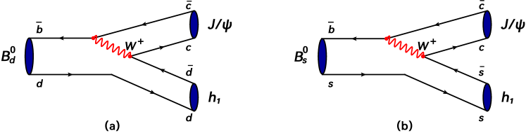
Figure 1: (Color online) Leading quark-level Feynman diagrams for $B^{0}\to J/\psi h_{1}$

In this article, we will systematically study the $B^{0}\to J/\psi h_{1}$ decays ($B^{0}$ includes $B_{d}^{0}$ and $B_{s}^{0}$), and further search for new observables for determining the mixing angle $\theta$ in $h_{1}$ states. The corresponding transition processes at the quark level are illustrated in Fig. 1. Several groups have studied the $B$-meson decays into a charmonium state Chen:2005ht ; Li:2007xf ; Li:2012sw ; Liu:2014doa ; Yao:2022zom ; Liu:2019ymi ; Cheng:2000kt ; Sun:2013dla ; Song:2002gw ; Meng:2005er ; Li:2006vq ; Beneke:2008pi ; Colangelo:2010wg ; Liu:2013nea ; Wang:2015uea ; Zhang:2017cbi ; Rui:2019yxx ; Li:2020app , and found that, in order to obtain reliable theoretical predictions for these color-suppressed transitions that are compatible with the current data, the next-to-leading order (NLO) QCD corrections, especially the vertex contributions, and the associated NLO Wilson coefficients, have to be taken into account in the related calculations. Besides, it is worth mentioning that the Sudakov factor for charmonia has been derived recently Liu:2018kuo ; Liu:2020upy ; Liu:2023kxr and will also be taken into account in this work. Combined with the above new ingredients, we will provide theoretical predictions for the first time on several observables of $B^{0}\to J/\psi h_{1}$, e.g., CP-averaged branching ratios, polarization fractions, relative phases, CP-violating asymmetries, and so on, by using the PQCD approach Keum:2000ph ; Keum:2000wi ; Lu:2000em ; Lu:2000hj ; Ali:2007ff ; Chai:2022ptk up to NLO accuracy. Comparing with the experimental data, the branching ratios and several interesting ratios could help us to effectively constrain the range of mixing angle $\theta$, and can provide more useful information for identifying the inner structure of the $h_{1}$ states.

This paper is organized as follows. In Sect. II, we overview briefly the mixing angle of axial-vector $h_{1}$ mesons indirectly through the Gell-Mann$-$Okubo mass relations, and then present the analytic expressions for the $B^{0}\to J/\psi h_{1}$ decay amplitudes in the PQCD approach. In Sect. III, the values of requisite input parameters are collected, the theoretical results are given and the phenomenological discussions are made in detail. Finally, we give our summary in Sect. IV.

II Formalism and Perturbative QCD calculations

II.1 The mixing angle

It is known that the physical eigenstates $K_{1}(1270)$ and $K_{1}(1400)$ are treated as the mixtures of $K_{1A}$ and $K_{1B}$, which can be expressed as Suzuki:1993yc

$$\left(\begin{array}[]{c}K_{1}(1270)\\ K_{1}(1400)\\ \end{array}\right)=\left(\begin{array}[]{cc}\sin{\theta}_{K}&\,\,\cos{\theta}_{K}\\ \cos{\theta}_{K}&-\sin{\theta}_{K}\end{array}\right)\left(\begin{array}[]{c}{K}_{1A}\\ {K}_{1B}\\ \end{array}\right)\;,$$ (19)

where $\theta_{K}$ is the mixing angle.

Table 1: Theoretical predictions for $\theta_{K}$

Models	Results of $\theta_{K}$
SO basis Cheng:2013cwa ; Gao:2019jme	$\theta_{K}=33^{\circ}$
	$\theta_{K}=(42.6\pm 2.2)^{\circ}$
QF basis Suzuki:1993yc ; Divotgey:2013jba	$\theta_{K}\approx 33^{\circ}$
	$\theta_{K}=(33.6\pm 4.3)^{\circ}$
NRQM Burakovsky:1997dd ; Burakovsky:1997ci	$35^{\circ}\leq\theta_{K}\leq 55^{\circ}$
	$\theta_{K}=(37.3\pm 3.2)^{\circ}$
QCD Sum Rules Dag:2012zz	$\theta_{K}=(39\pm 4)^{\circ}$
Relativized QM Blundell:1995au	$\theta_{K}\approx 45^{\circ}$
Average	$\theta_{K}\approx 39^{\circ}$

The value of mixing angle $\theta_{K}$ has been studied in the previous works. Using the early experimental information of $\tau$ decays, the authors of Ref. Suzuki:1993yc obtain two solutions $\theta_{K}\approx 33^{\circ}$ or $57^{\circ}$, and present that the observed $K_{1}(1400)$ production dominance in the $\tau$ decay favors $\theta_{K}\approx 33^{\circ}$, while $\theta_{K}=(42.6\pm 2.2)^{\circ}$ is obtained in Ref. Gao:2019jme by using BESIII measured $M_{h_{1}(1415)}=(1423.2\pm 7.6)\,{\rm MeV}$, which is larger than the last BESIII measurement $M_{h_{1}(1415)}=(1384\pm 6)\,{\rm MeV}$ BESIII:2022zel . The phenomenological analysis of the $\tau\to K_{1}\nu_{\tau}$ decay suggested that $\theta_{K}\approx 45^{\circ}$ Blundell:1995au in the relativized quark model. In Ref. Cheng:2013cwa , the author again reinforces the statement that a relatively small $\theta_{K}=33^{\circ}$ is much more favored by the lattice and phenomenological analyses. In the nonrelativistic quark model, the range $35^{\circ}\leq\theta_{K}\leq 55^{\circ}$ Burakovsky:1997dd is obtained, and a refined result $\theta_{K}=(37.3\pm 3.2)^{\circ}$ Burakovsky:1997ci is given by using the masses of $b_{1}(1235)$ and $a_{1}(1260)$ mesons. A similar result $\theta_{K}=(39\pm 4)^{\circ}$ Dag:2012zz is obtained by calculating a two-point correlation function related to $\theta_{K}$ within QCD sum rules. The results mentioned above are collected in Table 1, and their average value is $\theta_{K}=39^{\circ}$. Then, we would like to clarify the way to obtain the value of mixing angle $\theta$ by using $\theta_{K}$.

Applying the Gell-Mann$-$Okubo relations (specific pedagogical conclusions can be found in Appendix A), the mass squared of the octet state can be written as

$$m_{\tilde{h}_{8}}^{2}=\frac{4m_{K_{1B}}^{2}-m_{b_{1}}^{2}}{3}\;,$$ (20)

where $K_{1B}$ and $b_{1}$ are light meson states belonging to the ${}^{1}P_{1}$ nonet. The mixing angle $\theta$ can thus be obtained by

$$\cos^{2}\theta=\frac{4m_{K_{1B}}^{2}-m_{b_{1}}^{2}-3m_{h_{1}(1170)}^{2}}{3\left(m_{h_{1}(1415)}^{2}-m_{h_{1}(1170)}^{2}\right)}\;,\qquad\tan\theta=\frac{4m_{K_{1B}}^{2}-m_{b_{1}}^{2}-3m_{h_{1}(1415)}^{2}}{2\sqrt{2}\left(m_{b_{1}}^{2}-m_{K_{1B}}^{2}\right)}\;.$$ (21)

The PDG results for the masses of physical states are used in our evaluation. It can be found that, for a given $\theta_{K}$, the corresponding value of mixing angle $\theta$ can be extracted via the above formulae, and the value of $\alpha$ can also be obtained by using Eq. (12). Using some possible values of $\theta_{K}$ as inputs, we give the results of $\theta$ and $\alpha$ in Table 2. The default value $\theta=29.5^{\circ}$ used in our following calculations corresponds to $\theta_{K}=39^{\circ}$. As has been shown in Eq. (11), the mixing angle $\theta$ plays an important role in the investigation of $h_{1}$ mesons, thus the effects of $\theta$ on our theoretical predictions are also discussed in our following analyses.

Table 2: The values of mixing angles of $h_{1}$ mesons in the QF (upper) and SO (lower) basis with some possible values of $\theta_{K}$ as inputs.

$|\theta_{K}|$	$27^{\circ}$	$33^{\circ}$	$39^{\circ}$	$45^{\circ}$	$51^{\circ}$	$57^{\circ}$
$\alpha-90^{\circ}$	$3.2^{\circ}$	$-0.8^{\circ}$	$-5.8^{\circ}$	$-10.9^{\circ}$	$-17.5^{\circ}$	$-27.1^{\circ}$
$\theta$	$38.5^{\circ}$	$34.5^{\circ}$	$29.5^{\circ}$	$24.4^{\circ}$	$17.8^{\circ}$	$8.2^{\circ}$

II.2 The $B^{0}\to J/\psi h_{1}$ decays in PQCD approach

The PQCD approach is one of the popular factorization approaches on the basis of QCD, and has been widely employed to study a variety of $B$-meson decays. Recently, the NLO PQCD predictions of the CP-averaged branching ratios for the $B^{0}$-meson decays into a charmonium plus light hadrons have been improved through including the important vertex corrections Liu:2014doa ; Liu:2019ymi ; Yao:2022zom ; Xiao:2019mpm ; Ren:2023ebq . It makes this work a possible reference for future experimental measurements and may provide a solid theoretical basis for exploring the possible new physics beyond the SM potentially.

For the considered $B^{0}\to J/\psi h_{1}$ decays, the effective Hamiltonian can be written as Buchalla:1995vs

$$H_{\rm eff}\, = \,\frac{G_{F}}{\sqrt{2}}\left\{V^{*}_{cb}V_{cq}\biggl{[}C_{1}(\mu)O_{1}^{c}(\mu)+C_{2}(\mu)O_{2}^{c}(\mu)\biggr{]}-V^{*}_{tb}V_{tq}\biggl{[}\sum_{i=3}^{10}C_{i}(\mu)O_{i}(\mu)\biggr{]}\right\}\;,$$ (22)

where $q=d$ or $s$, the Fermi constant $G_{F}=1.16639\times 10^{-5}{\rm GeV}^{-2}$, $V$ stands for the Cabibbo-Kobayashi-Maskawa (CKM) matrix elements, and $C_{i}(\mu)$ are Wilson coefficients at the renormalization scale $\mu$. The local four-quark operators $O_{i}(i=1,\cdots,10)$ are given as

1. (1) Tree operators

   $${\begin{array}[]{ll}\displaystyle O_{1}^{c}\,=\,(\bar{q}_{\alpha}c_{\beta})_{V-A}(\bar{c}_{\beta}b_{\alpha})_{V-A}\;,&\displaystyle O_{2}^{c}\,=\,(\bar{q}_{\alpha}c_{\alpha})_{V-A}(\bar{c}_{\beta}b_{\beta})_{V-A}\;,\end{array}}$$ (24)

2. (2) QCD penguin operators

   $${\begin{array}[]{ll}\displaystyle O_{3}\,=\,(\bar{q}_{\alpha}b_{\alpha})_{V-A}\sum_{q^{\prime}}(\bar{q}^{\prime}_{\beta}q^{\prime}_{\beta})_{V-A}\;,&\displaystyle O_{4}\,=\,(\bar{q}_{\alpha}b_{\beta})_{V-A}\sum_{q^{\prime}}(\bar{q}^{\prime}_{\beta}q^{\prime}_{\alpha})_{V-A}\;,\\ \displaystyle O_{5}\,=\,(\bar{q}_{\alpha}b_{\alpha})_{V-A}\sum_{q^{\prime}}(\bar{q}^{\prime}_{\beta}q^{\prime}_{\beta})_{V+A}\;,&\displaystyle O_{6}\,=\,(\bar{q}_{\alpha}b_{\beta})_{V-A}\sum_{q^{\prime}}(\bar{q}^{\prime}_{\beta}q^{\prime}_{\alpha})_{V+A}\;,\end{array}}$$ (27)

3. (3) Electroweak penguin operators

   $${\begin{array}[]{ll}\displaystyle O_{7}\,=\,\frac{3}{2}(\bar{q}_{\alpha}b_{\alpha})_{V-A}\sum_{q^{\prime}}e_{q^{\prime}}(\bar{q}^{\prime}_{\beta}q^{\prime}_{\beta})_{V+A}\;,&\displaystyle O_{8}\,=\,\frac{3}{2}(\bar{q}_{\alpha}b_{\beta})_{V-A}\sum_{q^{\prime}}e_{q^{\prime}}(\bar{q}^{\prime}_{\beta}q^{\prime}_{\alpha})_{V+A}\;,\\ \displaystyle O_{9}\,=\,\frac{3}{2}(\bar{q}_{\alpha}b_{\alpha})_{V-A}\sum_{q^{\prime}}e_{q^{\prime}}(\bar{q}^{\prime}_{\beta}q^{\prime}_{\beta})_{V-A}\;,&\displaystyle O_{10}\,=\,\frac{3}{2}(\bar{q}_{\alpha}b_{\beta})_{V-A}\sum_{q^{\prime}}e_{q^{\prime}}(\bar{q}^{\prime}_{\beta}q^{\prime}_{\alpha})_{V-A}\;,\end{array}}$$ (30)

with the color indices $\alpha,\beta$ and the notations $V\pm A=\gamma_{\mu}(1\pm\gamma_{5})$. The index $q^{\prime}$ in the summation of the above operators runs through $u,\;d,\;s$, $c$ and $b$. For convenience, the combination $a_{i}$ of Wilson coefficients are defined as Liu:2013nea ; Ali:2007ff

$$a_{1} = C_{2}+\frac{C_{1}}{3}\;,\qquad a_{2}=C_{1}+\frac{C_{2}}{3}\;,$$ (31)

and

$$a_{i} = C_{i}+\frac{C_{i\pm 1}}{3}\quad(i=3-10)\;,$$ (32)

in which the upper(lower) sign applies, when $i$ is odd(even).

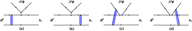
Figure 2: (Color online) Leading order Feynman diagrams for $B^{0}\to J/\psi h_{1}$ in the PQCD approach.

In Fig. 2, we show the typical Feynman diagrams contributing to the $B^{0}\to J/\psi h_{1}$ decays in the PQCD approach at leading order (LO), with the first two factorizable emission diagrams and the last two non-factorizable emission ones. Consequently, analogous to the decays $B^{0}\to J/\psi V$ Liu:2013nea , the specific forms of the factorizable emission amplitude $F_{J/\psi}^{h}$ ($h$ stands for three polarizations of the final (axial-) vector states: longitudinal ($L$), normal ($N$), and transverse ($T$), respectively.) and the non-factorizable emission amplitude $M_{J/\psi}^{h}$ are given as

$$F_{J/\psi}^{L} = 8\pi C_{F}f_{J/\psi}m_{B^{0}}^{4}\int_{0}^{1}dx_{1}dx_{3}\int_{0}^{\infty}b_{1}db_{1}b_{3}db_{3}\phi_{B}(x_{1},b_{1})\biggl{\{}\Bigl{[}\sqrt{1-r_{2}^{2}}\bigl{(}r_{A}\bigl{(}\sqrt{1-r_{2}^{2}}$$ (33)

$$\times(2x_{3}-1)\phi_{A}^{s}(x_{3})-\phi_{A}^{t}(x_{3})(2x_{3}(r_{2}^{2}-1)+r_{2}^{2}+1)\bigr{)}+\phi_{A}(x_{3})\bigl{(}(r_{2}^{2}-1)x_{3}-1\bigr{)}\bigr{)}\Bigr{]}$$

$$\times h_{fe}(x_{1},x_{3},b_{1},b_{3})E_{fe}(t_{a})-\Bigl{[}2r_{A}(1-r_{2}^{2})\phi_{A}^{s}(x_{3})\Bigr{]}h_{fe}(x_{3},x_{1},b_{3},b_{1})E_{fe}(t_{b})\biggr{\}}\;,$$

$$F_{J/\psi}^{N} = 8\pi C_{F}f_{J/\psi}m_{B^{0}}^{4}\int_{0}^{1}dx_{1}dx_{3}\int_{0}^{\infty}b_{1}db_{1}b_{3}db_{3}\phi_{B}(x_{1},b_{1})r_{2}\biggl{\{}\Bigl{[}(r_{2}^{2}-1)\bigl{[}r_{A}(r_{2}^{2}-1)x_{3}$$ (34)

$$\times\phi_{A}^{a}(x_{3})+\phi_{A}^{T}(x_{3})\bigr{]}+r_{A}\bigl{[}(r_{2}^{2}-1)x_{3}-2\bigr{]}\phi_{A}^{v}(x_{3})\Bigr{]}h_{fe}(x_{1},x_{3},b_{1},b_{3})E_{fe}(t_{a})$$

$$-r_{A}(r_{2}^{2}-1)\Bigl{[}(r_{2}^{2}-1)\phi_{A}^{a}(x_{3})-\phi_{A}^{v}(x_{3})\Bigr{]}h_{fe}(x_{3},x_{1},b_{3},b_{1})E_{fe}(t_{b})\biggr{\}}\;,$$

$$F_{J/\psi}^{T} = 16\pi C_{F}f_{J/\psi}m_{B^{0}}^{4}\int_{0}^{1}dx_{1}dx_{3}\int_{0}^{\infty}b_{1}db_{1}b_{3}db_{3}\phi_{B}(x_{1},b_{1})r_{2}$$ (35)

$$\times\biggl{\{}\Bigl{[}r_{A}x_{3}\phi_{A}^{v}(x_{3})-\phi_{A}^{T}(x_{3})+r_{A}\bigl{[}(r_{2}^{2}-1)x_{3}-2\bigr{]}\phi_{A}^{a}(x_{3})\Bigr{]}h_{fe}(x_{1},x_{3},b_{1},b_{3})E_{fe}(t_{a})$$

$$+r_{A}\Bigl{[}(r_{2}^{2}-1)\phi_{A}^{a}(x_{3})-\phi_{A}^{v}(x_{3})\Bigr{]}h_{fe}(x_{3},x_{1},b_{3},b_{1})E_{fe}(t_{b})\biggr{\}}\;,$$

with $r_{A}=m_{\tilde{h}_{1(8)}}/m_{B^{0}}$ and $r_{2}=m_{J/\psi}/m_{B^{0}}$, and

$$M_{J/\psi}^{L} = \frac{16\sqrt{6}}{3}\pi C_{F}m_{B^{0}}^{4}\int_{0}^{1}dx_{1}dx_{2}dx_{3}\int_{0}^{\infty}b_{1}db_{1}b_{2}db_{2}\phi_{B}(x_{1},b_{1})$$ (36)

$$\times\biggl{\{}\Bigl{[}\sqrt{1-r_{2}^{2}}\bigl{(}\phi_{A}(x_{3})-2r_{A}\phi_{A}^{t}(x_{3})\bigr{)}\bigl{(}r_{2}^{2}\phi_{J/\psi}^{L}(x_{2})(2x_{2}-x_{3})$$

$$+x_{3}\phi_{J/\psi}^{L}(x_{2})-2r_{2}r_{c}\phi_{J/\psi}^{t}(x_{2})\bigr{)}\Bigr{]}\biggr{\}}h_{nfe}(x_{1},x_{2},x_{3},b_{1},b_{2})E_{nfe}(t_{nfe})\;,$$

$$M_{J/\psi}^{N} = \frac{32\sqrt{6}}{3}\pi C_{F}m_{B^{0}}^{4}\int_{0}^{1}dx_{1}dx_{2}dx_{3}\int_{0}^{\infty}b_{1}db_{1}b_{2}db_{2}\phi_{B}(x_{1},b_{1})$$ (37)

$$\times\biggl{\{}(r_{2}^{2}-1)\Bigl{[}r_{2}x_{2}\phi_{J/\psi}^{v}(x_{2})-r_{c}\phi_{J/\psi}^{T}(x_{2})\Bigr{]}\phi_{A}^{T}(x_{3})+r_{A}\Bigl{[}-r_{c}(1+r_{2}^{2})\phi_{J/\psi}^{T}(x_{2})$$

$$+r_{2}\bigl{[}x_{2}(1+r_{2}^{2})+x_{3}(1-r_{2}^{2})\bigr{]}\phi_{J/\psi}^{v}(x_{2})\Bigr{]}\phi_{A}^{v}(x_{3})\biggr{\}}h_{nfe}(x_{1},x_{2},x_{3},b_{1},b_{2})E_{nfe}(t_{nfe})\;,$$

$$M_{J/\psi}^{T} = \frac{64\sqrt{6}}{3}\pi C_{F}m_{B^{0}}^{4}\int_{0}^{1}dx_{1}dx_{2}dx_{3}\int_{0}^{\infty}b_{1}db_{1}b_{2}db_{2}\phi_{B}(x_{1},b_{1})$$ (38)

$$\times\biggl{\{}\Bigl{[}r_{c}\phi_{J/\psi}^{T}(x_{2})-r_{2}x_{2}\phi_{J/\psi}^{v}(x_{2})\Bigr{]}\phi_{A}^{T}(x_{3})+r_{A}\Bigl{[}-r_{c}(1+r_{2}^{2})\phi_{J/\psi}^{T}(x_{2})+r_{2}\bigl{[}x_{2}(1+r_{2}^{2})$$

$$+x_{3}(1-r_{2}^{2})\bigr{]}\phi_{J/\psi}^{v}(x_{2})\Bigr{]}\phi_{A}^{a}(x_{3})\biggr{\}}h_{nfe}(x_{1},x_{2},x_{3},b_{1},b_{2})E_{nfe}(t_{nfe})\;,$$

where $r_{c}=m_{c}/m_{B^{0}}$ with $m_{c}$ being the charm quark mass. For the sake of simplicity, the explicit forms of hard function $h(x_{i},b_{i})$, evolution function $E_{i}(t)$ and the running hard scale $t$ of $F_{J/\psi}^{h}$ and $M_{J/\psi}^{h}$ in the above equations (33)-(38) can be referred to the Refs. Liu:2013nea ; Ren:2023ebq .

As has been emphasized in the introduction, the color-suppressed $B^{0}\to J/\psi h_{1}$ decays should include the known NLO contributions from vertex corrections and NLO Wilson coefficients to improve the accuracy of the theoretical predictions. The corresponding vertex corrections have been shown in Fig. 3, and will be considered in our calculation. As has been pointed out in Chen:2005ht ; Cheng:2000kt , their effects can be absorbed into the Wilson coefficients of factorizable contributions and subsequently form a set of effective Wilson coefficients $\tilde{a}_{i}^{\sigma}(i=2,3,5,7,9)$ with helicities $(\sigma=0,\pm)$. The explicit expressions of $\tilde{a}_{i}^{\sigma}$ can be found in Ref. Yao:2022zom .

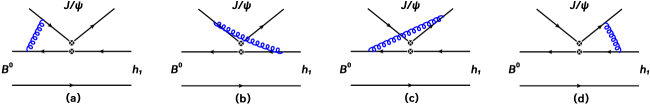
Figure 3: (Color online) Vertex corrections to $B^{0}\to J/\psi h_{1}$ at NLO

In the PQCD calculations at LO accuracy, we shall use the LO Wilson coefficients $C_{i}(m_{W})$, the LO renormalization group (RG) evolution matrix $U(t,m)^{(0)}$ for the Wilson coefficient with the LO running coupling $\alpha_{s}(t)^{(0)}$,

$$\alpha_{s}(t)^{(0)}=\frac{4\pi}{\beta_{0}\ln\left(t^{2}/\Lambda_{\rm QCD}^{2}\right)}\;,$$ (39)

where $\beta_{0}=(33-2N_{f})/3$. While, the NLO Wilson coefficients $C_{i}(m_{W})$ and the NLO RG evolution matrix $U(t,m,\alpha)$ with the running coupling $\alpha_{s}(t)$ at two-loop level should be used in the PQCD calculations at the NLO accuracy Buchalla:1995vs ,

$$\alpha_{s}(t)=\frac{4\pi}{\beta_{0}\ln\left(t^{2}/\Lambda_{\rm QCD}^{2}\right)}\,\Biggl{\{}1-\frac{\beta_{1}}{\beta_{0}^{2}}\cdot\frac{\ln\left[\ln\left(t^{2}/\Lambda_{\rm QCD}^{2}\right)\right]}{\ln\left(t^{2}/\Lambda_{\rm QCD}^{2}\right)}\Biggr{\}}\;,$$ (40)

where $\beta_{0}=(33-2N_{f})/3$ and $\beta_{1}=(306-38N_{f})/3$. The hadronic scale $\Lambda_{\rm QCD}^{(4)}=0.287$ GeV (0.326 GeV) could be obtained by using $\Lambda_{\rm QCD}^{(5)}=0.225$ GeV for the LO (NLO) case Buchalla:1995vs . For the hard scale $t$, the lower cut-off $\mu_{0}=1.0$ GeV is chosen Xiao:2008sw .

Using the building-blocks given above, the decay amplitudes of $B^{0}\to J/\psi\tilde{h}_{1(8)}$ can then be written as

$$A^{h}(B_{d,s}^{0}\to J/\psi\tilde{h}_{1(8)}) = F_{J/\psi}^{h}\Biggl{\{}V_{cb}^{\ast}V_{cd(s)}\tilde{a}_{2}^{\sigma}-V_{tb}^{\ast}V_{td(s)}\biggl{(}\tilde{a}_{3}^{\sigma}+\tilde{a}_{5}^{\sigma}+\tilde{a}_{7}^{\sigma}+\tilde{a}_{9}^{\sigma}\biggr{)}\Biggr{\}}$$ (41)

$$+M_{J/\psi}^{h}\Biggl{\{}V_{cb}^{\ast}V_{cd(s)}C_{2}-V_{tb}^{\ast}V_{td(s)}\biggl{(}C_{4}-C_{6}-C_{8}+C_{10}\biggr{)}\Biggr{\}}\;,$$

with the superscripts $h$ and $\sigma$ representing the polarization and helicity of the final states, respectively. Specifically, $h=L$ corresponds to a helicity $\sigma=0$, while $h=N,T$ corresponds to helicities $\sigma=\pm$. Combining various contributions from different Feynman diagrams and the single-octet mixing scheme as given in Eq. (11), the decay amplitudes of the considered $B^{0}\to J/\psi h_{1}$ decays with physical states could be expressed as follows,

• For $B_{d}^{0}\to J/\psi h_{1}$ decays,

  $${\cal A}^{h}\left(B_{d}^{0}\to J/\psi h_{1}(1170)\right) = \;A^{h}\left(B_{d}^{0}\to J/\psi\tilde{h}_{1}\right)\frac{\cos\theta}{\sqrt{3}}+A^{h}\left(B_{d}^{0}\to J/\psi\tilde{h}_{8}\right)\frac{\sin\theta}{\sqrt{6}}\;,$$ (42)

  $${\cal A}^{h}\left(B_{d}^{0}\to J/\psi h_{1}(1415)\right) = \;A^{h}\left(B_{d}^{0}\to J/\psi\tilde{h}_{8}\right)\frac{\cos\theta}{\sqrt{6}}-A^{h}\left(B_{d}^{0}\to J/\psi\tilde{h}_{1}\right)\frac{\sin\theta}{\sqrt{3}}\;,$$ (43)

• For $B_{s}^{0}\to J/\psi h_{1}$ decays,

  $${\cal A}^{h}\left(B_{s}^{0}\to J/\psi h_{1}(1170)\right) = \;A^{h}\left(B_{s}^{0}\to J/\psi\tilde{h}_{1}\right)\frac{\cos\theta}{\sqrt{3}}-2A^{h}\left(B_{s}^{0}\to J/\psi\tilde{h}_{8}\right)\frac{\sin\theta}{\sqrt{6}}\;,$$ (44)

  $${\cal A}^{h}\left(B_{s}^{0}\to J/\psi h_{1}(1415)\right) = -2A^{h}\left(B_{s}^{0}\to J/\psi\tilde{h}_{8}\right)\frac{\cos\theta}{\sqrt{6}}-A^{h}\left(B_{s}^{0}\to J/\psi\tilde{h}_{1}\right)\frac{\sin\theta}{\sqrt{3}}\;.\;\;$$ (45)

III Numerical results and discussions

Table 3: The values of input parameters.

Masses (GeV)	$m_{B_{d}^{0}}=5.28$ , $m_{B_{s}^{0}}=5.37$ , $m_{b}=4.8$ , $m_{c}=1.50$ , $m_{J/\psi}=3.097$ ,
	$m_{h_{1}(1170)}=1.166$ , $m_{h_{1}(1415)}=1.409$ ,  $m_{\tilde{h}_{1}}=1.23$ ,  $m_{\tilde{h}_{8}}=1.36$
Decay constants (GeV)	$f_{B_{d}^{0}}=0.21\pm 0.02$ , $f_{B_{s}^{0}}=0.23\pm 0.02$ , $f_{J/\psi}=0.405\pm 0.014$ ,
	$f_{\tilde{h}_{1}}=0.180\pm 0.012$ , $f_{\tilde{h}_{8}}=0.190\pm 0.010$
$B$-meson lifetimes (ps)	$\tau_{B_{d}^{0}}=1.519\pm 0.004$ , $\tau_{B_{s}^{0}}=1.520\pm 0.005$
CKM parameters	$A=0.826^{+0.018}_{-0.015}$ , $\lambda=0.22500\pm 0.00067$ ,  $\bar{\rho}=0.159\pm 0.010$ ,
	$\bar{\eta}=0.348\pm 0.010$

In the numerical calculations, the meson masses, decay constants, $B^{0}$ meson lifetimes, and CKM matrix elements (Wolfenstein parameters Wolfenstein:1983yz ) are essential input parameters. Their values ParticleDataGroup:2022pth ; Yang:2007zt ; Verma:2011yw are collected in Table 3. For the nonleptonic two-body $B^{0}\to J/\psi h_{1}$ decays, the branching fraction ${\cal B}$ is defined as

$${\cal B} \equiv \tau_{B^{0}}\cdot\Gamma\left(B^{0}\to J/\psi h_{1}\right)=\tau_{B^{0}}\cdot\frac{G_{F}^{2}\left|\bf{P_{c}}\right|}{16\pi m^{2}_{B^{0}}}\sum_{h=L,N,T}{\cal A}^{(h)\dagger}{\cal A}^{(h)}\;,$$ (46)

where $\tau_{B^{0}}$ is the lifetime of $B^{0}$-meson, $|\bf{P_{c}}|\equiv|\bf{P_{2z}}|=|\bf{P_{3z}}|$ is the three-momentum of outgoing final states, and ${\cal A}^{h}$ denotes the helicity amplitudes of $B^{0}\to J/\psi h_{1}$ decays given in Eqs. (42)-(45).

Using the decay amplitudes and input parameters given above, our LO and NLO PQCD predictions for the CP-averaged branching fractions of $B^{0}\to J/\psi h_{1}$ decays, accompanied with multiple uncertainties, are given in Table 4. The first four theoretical errors are induced by the shape parameter $\omega_{B_{d}^{0}}=0.40\pm 0.04$ GeV or $\omega_{B_{s}^{0}}=0.50\pm 0.05$ GeV in the $B^{0}$-meson distribution amplitude, the decay constant $f_{M}$ of two outgoing final states as presented in Table 3, the charm quark mass $m_{c}=1.50\pm 0.15$ GeV, and the Gegenbauer moments $a_{1}^{\parallel}$ and $a_{2}^{\perp}$ (see Eq. (107)) in the light-cone distribution amplitudes of the $h_{1}$ mesons, respectively. The last error arises from factor $a_{t}=1.0\pm 0.2$ describing the possible higher-order corrections, which are characterized through simply varying the running hard scale $t_{\rm max}$ with $20\%$ in the hard kernel. From Table 4, it can be clearly seen that the dominated uncertainties arise mainly from the hadronic parameters such as the Gegenbauer moments and the decay constants.

Table 4: The LO and NLO PQCD predictions of the CP-averaged branching ratios for the $B^{0}\to J/\psi h_{1}$ decays.

Decay modes	LO	NLO
$B_{d}^{0}\to J/\psi h_{1}(1170)$	$\begin{array}[]{cc}\left(6.55_{-1.35-0.91-0.90-1.31-1.60}^{+1.78+0.96+1.20+1.58+2.23}\right)\times 10^{-5}\end{array}$	$\begin{array}[]{cc}\left(9.54_{-1.87-1.54-0.74-2.43-0.38}^{+2.39+1.65+0.72+2.83+0.26}\right)\times 10^{-5}\end{array}$
$B_{d}^{0}\to J/\psi h_{1}(1415)$	$\begin{array}[]{cc}\left(1.12_{-0.26-0.08-0.08-0.17-0.32}^{+0.36+0.08+0.14+0.22+0.44}\right)\times 10^{-6}\end{array}$	$\begin{array}[]{cc}\left(1.32_{-0.26-0.15-0.13-0.35-0.07}^{+0.35+0.17+0.14+0.41+0.04}\right)\times 10^{-6}\end{array}$
$B_{s}^{0}\to J/\psi h_{1}(1170)$	$\begin{array}[]{cc}\left(0.90_{-0.20-0.23-0.03-0.22-0.05}^{+0.27+0.26+0.09+0.26+0.08}\right)\times 10^{-5}\end{array}$	$\begin{array}[]{cc}\left(1.50_{-0.32-0.39-0.03-0.38-0.02}^{+0.42+0.44+0.01+0.44+0.01}\right)\times 10^{-5}\end{array}$
$B_{s}^{0}\to J/\psi h_{1}(1415)$	$\begin{array}[]{cc}\left(1.05_{-0.23-0.14-0.06-0.30-0.04}^{+0.29+0.14+0.09+0.36+0.07}\right)\times 10^{-3}\end{array}$	$\begin{array}[]{cc}\left(1.74_{-0.39-0.22-0.02-0.51-0.02}^{+0.50+0.26+0.01+0.61+0.01}\right)\times 10^{-3}\end{array}$

Comparing the numerical results at LO with the ones at NLO, we find that the NLO contributions from vertex corrections can significantly enhance the branching ratios due to the corrected effective Wilson coefficient $\tilde{a}_{2}$ being much larger than the original one $a_{2}$ Cheng:2000kt ; Chen:2005ht . Furthermore, we also note that the error arisen from the running hard scale $t$ can be reduced from $30\%$ to $5\%$. Therefore, the subsequent numerical results and phenomenological analyses are all at the presently known NLO level, unless otherwise specified.

Adding the above-mentioned errors in quadrature, the NLO PQCD results for ${\cal B}(B^{0}\to J/\psi h_{1})$ can be written as

• For $\bar{b}\to c\bar{c}\bar{d}$ decays,

  $${\cal B}\left(B_{d}^{0}\to J/\psi h_{1}(1170)\right)=9.54_{-3.53}^{+4.13}\times 10^{-5},\;\;{\cal B}\left(B_{d}^{0}\to J/\psi h_{1}(1415)\right)=1.32_{-0.48}^{+0.58}\times 10^{-6},\;\;$$ (47)

• For $\bar{b}\to c\bar{c}\bar{s}$ decays,

  $${\cal B}\left(B_{s}^{0}\to J/\psi h_{1}(1170)\right)=1.50_{-0.63}^{+0.75}\times 10^{-5},\;\;{\cal B}\left(B_{s}^{0}\to J/\psi h_{1}(1415)\right)=1.74_{-0.68}^{+0.83}\times 10^{-3}.\;\;$$ (48)

From these results, it can be found that $B^{0}\to J/\psi h_{1}$ decays have relatively large branching ratios, which are around $10^{-6}\sim 10^{-3}$, and are possible to be measured at the ongoing LHCb and Belle-II experiments in the near future.

Table 5: Decay amplitudes (in units of $10^{-3}\;{\rm GeV}^{3})$ of the $B^{0}\to J/\psi h_{1}$ modes with three polarizations in the PQCD approach.

Decays		${\cal A}_{B_{d}^{0}}$		${\cal A}_{B_{s}^{0}}$
Contributions		Tree	Penguin	Tree	Penguin
	${\cal A}_{L}$	$-0.125-i0.529$	$-0.002-i0.013$	$0.026+i0.212$	$-0.001+i0.006$
$J/\psi h_{1}(1170)$	${\cal A}_{N}$	$-0.032-i0.143$	$0.000-i0.004$	$0.026+i0.034$	$0.000+i0.001$
	${\cal A}_{T}$	$-0.110-i0.394$	$-0.001-i0.010$	$0.080+i0.104$	$0.001+i0.003$
	${\cal A}_{L}$	$-0.021-i0.064$	$-0.000-i0.002$	$-0.296-i2.422$	$0.003-i0.061$
$J/\psi h_{1}(1415)$	${\cal A}_{N}$	$-0.002-i0.020$	$0.000-i0.001$	$-0.235-i0.410$	$-0.005-i0.010$
	${\cal A}_{T}$	$-0.008-i0.053$	$0.000-i0.002$	$-0.705-i1.227$	$-0.014-i0.030$

Table 6: Same as Table 5 but for neutral $B$-meson decays into $J/\psi\tilde{h}_{1}$ and $J/\psi\tilde{h}_{8}$.

Decays		$A_{B_{d}^{0}}$		$A_{B_{s}^{0}}$
Contributions		Tree	Penguin	Tree	Penguin
	${\cal A}_{L}$	$-0.170-i0.743$	$-0.003-i0.018$	$0.292+i2.384$	$-0.003+i0.060$
$J/\psi\tilde{h}_{1}$	${\cal A}_{N}$	$-0.047-i0.198$	$0.000-i0.005$	$0.239+i0.401$	$0.005+i0.010$
	${\cal A}_{T}$	$-0.159-i0.549$	$-0.001-i0.014$	$0.721+i1.204$	$0.014+i0.029$
	${\cal A}_{L}$	$-0.195-i0.775$	$-0.003-i0.019$	$0.300+i2.454$	$-0.003+i0.061$
$J/\psi\tilde{h}_{8}$	${\cal A}_{N}$	$-0.043-i0.214$	$0.000-i0.006$	$0.234+i0.401$	$0.005+i0.010$
	${\cal A}_{T}$	$-0.151-i0.549$	$-0.001-i0.015$	$0.704+i1.245$	$0.014+i0.030$

In order to see clearly the interferences between two final states $J/\psi\tilde{h}_{1}$ and $J/\psi\tilde{h}_{8}$, we also give the numerical results of polarization amplitudes of $B^{0}\to J/\psi h_{1}$ and $B^{0}\to J/\psi\tilde{h}_{1,8}$ modes in Tables 5 and 6, respectively. Meanwhile, the amplitudes induced by the tree operators and the penguin operators are also listed. These numerical results indicate that the considered decay modes are dominated by the tree diagrams, with only a few percent of penguin contaminations. Combined with Eqs. (42)-(45), it is evident to observe that the constructive or destructive interferences with different extents in the considered decays could vary with the mixing angle $\theta$ in the SO basis. Thus, in order to show the effects of mixing angle $\theta$, we plot the dependence of NLO PQCD predictions of ${\cal B}(B^{0}\to J/\psi h_{1})$ on the mixing angle $\theta\in[-\frac{\pi}{2},\frac{\pi}{2}]$ in Fig. 4. It can be clearly seen that the ${\cal B}(B^{0}\to J/\psi h_{1})$ are very sensitive to the mixing angle $\theta$. From the Eqs. (42)-(45) and Fig. 4, it can be clearly seen that the interference between the $B_{s}^{0}\to J/\psi\tilde{h}_{1}$ and $B_{s}^{0}\to J/\psi\tilde{h}_{8}$ decay amplitudes consequently leads to that ${\cal B}(B_{s}^{0}\to J/\psi h_{1}(1170),\,B_{d}^{0}\to J/\psi h_{1}(1415))$ are significantly reduced, while ${\cal B}(B_{d}^{0}\to J/\psi h_{1}(1170),\,B_{s}^{0}\to J/\psi h_{1}(1415))$ are enhanced, at $\theta\sim 29.5^{\circ}$. Therefore, the experimental measurement of these branching fractions would play an important role in testing the value of $\theta$.

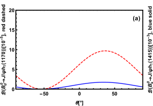
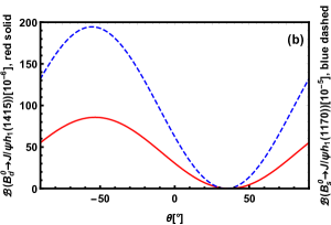
Figure 4: (Color online) The dependence of ${\cal B}(B^{0}\to J/\psi h_{1})$ on the mixing angle $\theta$ in the PQCD approach.

There are several unflavored light mesons, such as $a_{1}(1260),$ $f_{1}(1285),$ $\eta(1405),$ $f_{1}(1420)$ and $\eta(1475)$, that are known to decay into $K_{S}^{0}K^{\pm}\pi^{\mp}$, and that could in principle be produced in $B^{0}$ meson decays alongside charmonium states LHCb:2014sli . For the $h_{1}(1415)$ state below 1500 ${\rm MeV}/c^{2}$, the process $h_{1}(1415)\to K_{S}^{0}K^{\pm}\pi^{\mp}$ has not been measured ParticleDataGroup:2022pth . As discussed in Ref. Du:2021zdg , the decay rate of the dominant decay mode is ${\cal B}(h_{1}(1415)\to{K}^{\ast}\bar{K})=0.415\pm 0.085$, then the branching fraction ${\cal B}(h_{1}(1415)\to K_{S}^{0}K^{\pm}\pi^{\mp})\approx 0.277\pm 0.056$ can be naively determined due to the isospin conservation for the strong decays $K^{\ast}\to K\pi$. Based on the narrow-width-approximation (NWA), we can obtain the branching fractions of $B^{0}\to J/\psi h_{1}(1415)(\to K_{S}^{0}K^{+}\pi^{-})$ decays,

$${\cal B}\left(B_{s}^{0}\to J/\psi(K_{S}^{0}K^{+}\pi^{-})_{h_{1}(1415)}\right) \equiv {\cal B}\left(B_{s}^{0}\to J/\psi h_{1}(1415)\right)$$ (49)

$$\cdot{\cal B}\left(h_{1}(1415)\to K_{S}^{0}K^{+}\pi^{-}\right)\approx 0.48_{-0.21}^{+0.25}\times 10^{-3}\;,$$

$${\cal B}\left(B_{d}^{0}\to J/\psi(K_{S}^{0}K^{+}\pi^{-})_{h_{1}(1415)}\right) \equiv {\cal B}\left(B_{d}^{0}\to J/\psi h_{1}(1415)\right)$$ (50)

$$\cdot{\cal B}\left(h_{1}(1415)\to K_{S}^{0}K^{+}\pi^{-}\right)\approx 0.37_{-0.15}^{+0.18}\times 10^{-6}\;,$$

where the error arising from the $h_{1}(1415)$ decay width has been taken into account. As have been given in Ref. Yao:2022zom , the theoretical results for above processes through $f_{1}(1420)$ resonance showed that,

$${\cal B}(B_{s}^{0}\to J/\psi(K_{S}^{0}K^{+}\pi^{-})_{f_{1}(1420)})\approx 0.73_{-0.28}^{+0.36}\times 10^{-3}\;,$$ (51)

$${\cal B}(B_{d}^{0}\to J/\psi(K_{S}^{0}K^{+}\pi^{-})_{f_{1}(1420)})\approx 1.27_{-0.68}^{+0.88}\times 10^{-6}\;.$$ (52)

While, the $B^{0}\to J/\psi K_{S}^{0}K^{\pm}\pi^{\mp}$ decays have been measured by the LHCb Collaboration, their branching ratios are LHCb:2014sli

$${\cal B}(B_{s}^{0}\to J/\psi K_{S}^{0}K^{+}\pi^{-})_{\rm Exp} = (0.91\pm 0.09)\times 10^{-3}\;,$$ (53)

$${\cal B}(B_{d}^{0}\to J/\psi K_{S}^{0}K^{+}\pi^{-})_{\rm Exp} < 2.01\times 10^{-5}\;.$$ (54)

For the well measured $B_{s}^{0}\to J/\psi K_{S}^{0}K^{+}\pi^{-}$ decay, comparing the theoretical results given in Eqs. (49) and (51) with data given in Eq. (53), it can be found that the sum of the branching fractions of $B_{s}^{0}\to J/\psi K_{S}^{0}K^{+}\pi^{-}$ decay via $h_{1}(1415)$ and $f_{1}(1420)$ resonances is approximately consistent with the LHCb measurement of ${\cal B}(B_{s}^{0}\to J/\psi K_{S}^{0}K^{+}\pi^{-})$. However, considering the presently unknown interferences between the amplitudes from two different $f_{1}(1420)$ and $h_{1}(1415)$ resonant states, an accurate quantification of the $h_{1}(1415)$ resonance contributing to the $m(K_{S}^{0}K^{\pm}\pi^{\mp})$ distribution still requires further experimental and/or theoretical examinations on the interference effects.

As has been shown in Table 4, the branching fractions of the $B^{0}\to J/\psi h_{1}$ decays have relatively large theoretical uncertainties due to the various hadronic input parameters. Generally, the theoretical errors caused by the same hadronic input parameters can be significantly cancelled by introducing some ratios. For instance, one can define the following two ratios,

$$R_{d}^{\rm SO} \equiv \frac{{\cal B}\left(B_{d}^{0}\to J/\psi h_{1}(1170)\right)}{{\cal B}\left(B_{d}^{0}\to J/\psi h_{1}(1415)\right)}$$ (55)

$$= \frac{\Phi\left(m_{B_{d}^{0}},m_{J/\psi},m_{h_{1}(1170)}\right)}{\Phi\left(m_{B_{d}^{0}},m_{J/\psi},m_{h_{1}(1415)}\right)}\cdot\frac{\left|\frac{\cos\theta}{\sqrt{3}}\cdot A(B_{d}^{0}\to J/\psi\tilde{h}_{1})+\frac{\sin\theta}{\sqrt{6}}\cdot A(B_{d}^{0}\to J/\psi\tilde{h}_{8})\right|^{2}}{\left|-\frac{\sin\theta}{\sqrt{3}}\cdot A(B_{d}^{0}\to J/\psi\tilde{h}_{1})+\frac{\cos\theta}{\sqrt{6}}\cdot A(B_{d}^{0}\to J/\psi\tilde{h}_{8})\right|^{2}}\;,$$

$$R_{s}^{\rm SO} \equiv \frac{{\cal B}\left(B_{s}^{0}\to J/\psi h_{1}(1415)\right)}{{\cal B}\left(B_{s}^{0}\to J/\psi h_{1}(1170)\right)}$$ (56)

$$= \frac{\Phi\left(m_{B_{s}^{0}},m_{J/\psi},m_{h_{1}(1415)}\right)}{\Phi\left(m_{B_{s}^{0}},m_{J/\psi},m_{h_{1}(1170)}\right)}\cdot\frac{\left|-\frac{\sin\theta}{\sqrt{3}}\cdot A(B_{s}^{0}\to J/\psi\tilde{h}_{1})-2\cdot\frac{\cos\theta}{\sqrt{6}}\cdot A(B_{s}^{0}\to J/\psi\tilde{h}_{8})\right|^{2}}{\left|\frac{\cos\theta}{\sqrt{3}}\cdot A(B_{s}^{0}\to J/\psi\tilde{h}_{1})-2\cdot\frac{\sin\theta}{\sqrt{6}}\cdot A(B_{s}^{0}\to J/\psi\tilde{h}_{8})\right|^{2}},\;\;$$

where the phase space factor is given as $\Phi(a,b,c)=[(a^{2}-(b+c)^{2})(a^{2}-(b-c)^{2})]^{\frac{1}{2}}$ Fleischer:2011au . It can be found that, these ratios can be used to test or extract the values of mixing angle $\theta$ approximately in a model independent way if $A(B^{0}\to J/\psi\tilde{h}_{1})=A(B^{0}\to J/\psi\tilde{h}_{8})$, which is approximately valid as has been shown through the numerical results given in Table 6. Our numerical results are

$$R_{d}^{\rm SO}=72.27_{-4.53}^{+3.59}\;,\qquad R_{s}^{\rm SO}=116.52_{-10.96}^{+10.46}\;.$$ (57)

It can be obviously found that the theoretical errors are significantly reduced. Moreover, in order to obtain a more intuitive interpretation, one can employ a more convenient and intuitive form by extending the ratios to the QF basis, which can be exactly derived as

$$R_{d}^{\rm QF}\equiv\frac{{\cal B}\left(B_{d}^{0}\to J/\psi h_{1}(1170)\right)}{{\cal B}\left(B_{d}^{0}\to J/\psi h_{1}(1415)\right)}=\frac{\Phi\left(m_{B_{d}},m_{J/\psi},m_{h_{1}(1170)}\right)}{\Phi\left(m_{B_{d}},m_{J/\psi},m_{h_{1}(1415)}\right)}\cdot\cot^{2}\alpha\;,$$ (58)

$$R_{s}^{\rm QF}\equiv\frac{{\cal B}\left(B_{s}^{0}\to J/\psi h_{1}(1415)\right)}{{\cal B}\left(B_{s}^{0}\to J/\psi h_{1}(1170)\right)}=\frac{\Phi\left(m_{B_{s}},m_{J/\psi},m_{h_{1}(1415)}\right)}{\Phi\left(m_{B_{s}},m_{J/\psi},m_{h_{1}(1170)}\right)}\cdot\cot^{2}\alpha\;,$$ (59)

where the ratios $R_{d}^{\rm QF}$ and $R_{s}^{\rm QF}$ are independent on the decay amplitudes. They could provide a much more convenient and clear way to extract the angle $\alpha$ when they are measured by the future experiments. The mixing angle $\theta$ can be further obtained via Eq. (12). Beside of the ratios mentioned above, the ratios defined as

$$R_{ds}^{\rm SO}[h_{1}(1170)]\equiv\frac{{\cal B}\left(B_{d}^{0}\to J/\psi h_{1}(1170)\right)}{{\cal B}\left(B_{s}^{0}\to J/\psi h_{1}(1170)\right)}\;,\qquad R_{sd}^{\rm SO}[h_{1}(1415)]\equiv\frac{{\cal B}\left(B_{s}^{0}\to J/\psi h_{1}(1415)\right)}{{\cal B}\left(B_{d}^{0}\to J/\psi h_{1}(1415)\right)}\;,$$ (60)

can also be used to constrain the absolute value of mixing angle $\theta$. Our numerical results are

$$R_{ds}^{\rm SO}[h_{1}(1170)]\approx 6.38_{-0.89}^{+1.17}\;,\qquad R_{sd}^{\rm SO}[h_{1}(1415)]\approx 13.18_{-1.92}^{+2.02}\times 10^{2}\;,$$ (61)

in which, all errors arising from various input parameters have been added in quadrature.

Now, we turn to investigate the polarization fractions of the $B^{0}\to J/\psi h_{1}$ decays. Based on the helicity amplitudes given in Eqs. (42)-(45), we can equivalently define a set of transversity amplitudes as follows,

$${\cal A}_{L} = m_{B^{0}}^{2}{\cal A}_{L}\;,\qquad{\cal A}_{\parallel}=\sqrt{2}m_{B^{0}}^{2}{\cal A}_{N}\;,\qquad{\cal A}_{\perp}=m_{J/\psi}m_{h_{1}}\sqrt{2({\kappa}^{2}-1)}{\cal A}_{T}\;,$$ (62)

for the longitudinal, parallel and perpendicular polarization states, respectively, with the ratio $\kappa=P_{2}\cdot P_{3}/(m_{J/\psi}m_{h_{1}})$. Then, we can define the polarization fractions as

$$f_{L,\parallel,\perp}\equiv\frac{|{\cal A}_{L,\parallel,\perp}|^{2}}{|{\cal A}_{L}|^{2}+|{\cal A}_{\parallel}|^{2}+|{\cal A}_{\perp}|^{2}}\;,\qquad f_{T}\equiv\frac{|{\cal A}_{\parallel}|^{2}+|{\cal A}_{\perp}|^{2}}{|{\cal A}_{L}|^{2}+|{\cal A}_{\parallel}|^{2}+|{\cal A}_{\perp}|^{2}}=f_{\parallel}+f_{\perp}\;,$$ (63)

which are obviously satisfy the relation $f_{L}+f_{\parallel}+f_{\perp}=f_{L}+f_{T}=1$. In addition, the relative phases $\phi_{\parallel}$ and $\phi_{\perp}$ (in units of rad) are defined as

$$\phi_{\parallel} = {\rm arg}\frac{{\cal A}_{\parallel}}{{\cal A}_{L}}\;,\qquad\phi_{\perp}={\rm arg}\frac{{\cal A}_{\perp}}{{\cal A}_{L}}\;.$$ (64)

Table 7: Theoretical predictions for the polarization observables of the $B_{d}^{0}\to J/\psi h_{1}$ decays.

Observables	$B_{d}^{0}\to J/\psi h_{1}(1170)$	$B_{d}^{0}\to J/\psi h_{1}(1415)$
$f_{L}(\%)$	$\begin{array}[]{ll}81.3_{-0.3-0.1-1.8-4.5-0.2}^{+0.3+0.1+1.3+3.6+0.2}\end{array}$	$\begin{array}[]{ll}80.3_{-0.6-0.1-1.7-3.8-0.4}^{+0.6+0.1+0.9+3.1+0.3}\end{array}$
$f_{\parallel}(\%)$	$\begin{array}[]{ll}11.8_{-0.2-0.1-0.6-2.1-0.1}^{+0.2+0.1+0.9+2.7+0.1}\end{array}$	$\begin{array}[]{ll}13.5_{-0.5-0.1-0.3-2.0-0.1}^{+0.5+0.1+1.1+2.4+0.2}\end{array}$
$f_{\perp}(\%)$	$\begin{array}[]{ll}\;\;6.9_{-0.1-0.0-0.7-1.5-0.1}^{+0.1+0.0+0.9+1.9+0.1}\end{array}$	$\begin{array}[]{ll}\;\;6.2_{-0.2-0.0-0.6-1.1-0.1}^{+0.2+0.0+0.7+1.5+0.2}\end{array}$
$\phi_{\parallel}({\rm rad})$	$\begin{array}[]{ll}3.16_{-0.02-0.00-0.13-0.10-0.00}^{+0.02+0.00+0.11+0.12+0.01}\end{array}$	$\begin{array}[]{ll}3.36_{-0.03-0.01-0.10-0.11-0.01}^{+0.02+0.01+0.07+0.13+0.01}\end{array}$
$\phi_{\perp}({\rm rad})$	$\begin{array}[]{ll}3.10_{-0.01-0.00-0.12-0.10-0.00}^{+0.01+0.00+0.09+0.13+0.00}\end{array}$	$\begin{array}[]{ll}3.30_{-0.01-0.01-0.09-0.11-0.01}^{+0.01+0.01+0.06+0.14+0.01}\end{array}$
${A}_{\rm CP}^{\rm dir,L}(10^{-2})$	$\begin{array}[]{ll}-0.81_{-0.05-0.02-0.02-0.09-0.44}^{+0.04+0.02+0.02+0.06+0.40}\end{array}$	$\begin{array}[]{ll}-1.05_{-0.06-0.03-0.05-0.10-0.44}^{+0.06+0.03+0.07+0.08+0.43}\end{array}$
${A}_{\rm CP}^{\rm dir,\parallel}(10^{-2})$	$\begin{array}[]{ll}-1.17_{-0.07-0.03-0.07-0.10-0.45}^{+0.07+0.03+0.07+0.12+0.42}\end{array}$	$\begin{array}[]{ll}-1.27_{-0.09-0.04-0.09-0.12-0.49}^{+0.08+0.04+0.10+0.14+0.45}\end{array}$
${A}_{\rm CP}^{\rm dir,\perp}(10^{-2})$	$\begin{array}[]{ll}-0.99_{-0.07-0.02-0.09-0.09-0.42}^{+0.06+0.02+0.07+0.11+0.39}\end{array}$	$\begin{array}[]{ll}-1.18_{-0.09-0.03-0.14-0.10-0.44}^{+0.09+0.03+0.13+0.15+0.43}\end{array}$

Table 8: Same as Table 7 but for $B_{s}^{0}\to J/\psi h_{1}$ decays.

Decay modes	$B_{s}^{0}\to J/\psi h_{1}(1170)$	$B_{s}^{0}\to J/\psi h_{1}(1415)$
$f_{L}(\%)$	$\begin{array}[]{ll}87.6_{-0.2-0.1-2.7-5.7-0.2}^{+0.3+0.1+2.7+4.5+0.2}\end{array}$	$\begin{array}[]{ll}89.4_{-0.3-0.0-2.8-5.9-0.1}^{+0.3+0.0+2.6+4.3+0.1}\end{array}$
$f_{\parallel}(\%)$	$\begin{array}[]{ll}\;\;7.1_{-0.2-0.1-1.5-2.6-0.1}^{+0.2+0.1+1.6+3.3+0.1}\end{array}$	$\begin{array}[]{ll}\;\;6.7_{-0.2-0.0-1.6-2.7-0.1}^{+0.2+0.0+1.8+3.7+0.1}\end{array}$
$f_{\perp}(\%)$	$\begin{array}[]{ll}\;\;5.3_{-0.1-0.0-1.2-1.9-0.1}^{+0.1+0.1+1.1+2.4+0.1}\end{array}$	$\begin{array}[]{ll}\;\;3.9_{-0.1-0.0-1.0-1.6-0.1}^{+0.1+0.0+1.0+2.2+0.1}\end{array}$
$\phi_{\parallel}({\rm rad})$	$\begin{array}[]{ll}2.61_{-0.01-0.01-0.19-0.07-0.01}^{+0.01+0.01+0.14+0.11+0.01}\end{array}$	$\begin{array}[]{ll}2.74_{-0.01-0.00-0.19-0.11-0.00}^{+0.01+0.00+0.16+0.16+0.01}\end{array}$
$\phi_{\perp}({\rm rad})$	$\begin{array}[]{ll}2.61_{-0.01-0.01-0.18-0.08-0.01}^{+0.01+0.01+0.15+0.11+0.01}\end{array}$	$\begin{array}[]{ll}2.74_{-0.01-0.00-0.19-0.11-0.00}^{+0.01+0.00+0.16+0.17+0.01}\end{array}$
${A}_{\rm CP}^{\rm dir,L}(10^{-4})$	$\begin{array}[]{ll}1.65_{-0.10-0.02-0.27-0.01-1.46}^{+0.02+0.03+0.48+0.01+1.86}\end{array}$	$\begin{array}[]{ll}1.37_{-0.01-0.01-0.09-0.00-1.66}^{+0.00+0.01+0.10+0.00+1.97}\end{array}$
${A}_{\rm CP}^{\rm dir,\parallel}(10^{-4})$	$\begin{array}[]{ll}1.64_{-0.14-0.06-0.20-0.71-1.18}^{+0.15+0.08+0.34+0.27+1.12}\end{array}$	$\begin{array}[]{ll}0.52_{-0.07-0.00-0.00-0.96-1.20}^{+0.09+0.00+0.11+0.63+1.39}\end{array}$
${A}_{\rm CP}^{\rm dir,\perp}(10^{-4})$	$\begin{array}[]{ll}1.55_{-0.09-0.06-0.11-0.72-0.97}^{+0.09+0.08+0.21+0.29+1.11}\end{array}$	$\begin{array}[]{ll}0.58_{-0.09-0.01-0.05-0.97-1.21}^{+0.09+0.01+0.07+0.59+1.37}\end{array}$

Our numerical results for the polarization observables of $B^{0}\to J/\psi h_{1}$ decays are given in Tables 7 and 8. Adding the errors in quadrature, the results of polarization fractions can be simplified as

$$f_{L}\left(B_{d}^{0}\to J/\psi h_{1}(1170)\right) = (81.3_{-4.9}^{+3.9})\%\;,\qquad f_{T}\left(B_{d}^{0}\to J/\psi h_{1}(1170)\right)=(18.7_{-2.7}^{+3.5})\%\;,$$ (65)

$$f_{L}\left(B_{d}^{0}\to J/\psi h_{1}(1415)\right) = (80.3_{-4.3}^{+3.2})\%\;,\qquad f_{T}\left(B_{d}^{0}\to J/\psi h_{1}(1415)\right)=(19.7_{-2.4}^{+3.1})\%\;,$$ (66)

and

$$f_{L}\left(B_{s}^{0}\to J/\psi h_{1}(1170)\right) = (87.6_{-6.3}^{+5.3})\%\;,\qquad f_{T}\left(B_{s}^{0}\to J/\psi h_{1}(1170)\right)=(12.4_{-3.7}^{+4.5})\%\;,$$ (67)

$$f_{L}\left(B_{s}^{0}\to J/\psi h_{1}(1415)\right) = (89.4_{-6.5}^{+5.0})\%\;,\qquad f_{T}\left(B_{s}^{0}\to J/\psi h_{1}(1415)\right)=(10.6_{-3.6}^{+4.7})\%\;,$$ (68)

It can be found that $f_{L}(B^{0}\to J/\psi h_{1})$ are generally larger than $80\%$, which indicate that $B^{0}\to J/\psi h_{1}$ decays are dominated by the longitudinal contributions. The dependence of ${f_{L}}(B^{0}\to J/\psi h_{1})$ on the mixing angle $\theta$ is shown in Fig. 5. It can be found that the polarization fractions generally are not sensitive to the value of $\theta$, except at $\theta\sim 35^{\circ}$ for $B_{d}^{0}\to J/\psi h_{1}(1415)$ and $B_{s}^{0}\to J/\psi h_{1}(1170)$ decays and at $\theta\sim-55^{\circ}$ for $B_{d}^{0}\to J/\psi h_{1}(1170)$ and $B_{s}^{0}\to J/\psi h_{1}(1415)$ decays. Thus, the polarization would present a very strong constraint on $\theta$ if a relatively small $f_{L}(B^{0}\to J/\psi h_{1})$ is observed by the experiments.

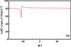
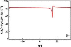
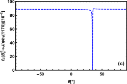
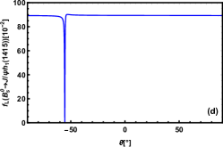
Figure 5: (Color online) The dependence of ${f_{L}}(B^{0}\to J/\psi h_{1})$ on the mixing angle $\theta$ in the PQCD approach.

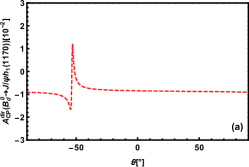
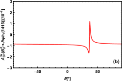
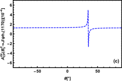
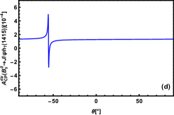
Figure 6: (Color online) The dependence of ${A_{\rm CP}^{\rm dir}}(B^{0}\to J/\psi h_{1})$ on the mixing angle $\theta$ in the PQCD approach.

The direct CP asymmetry $A_{\rm CP}^{\rm dir}$ of $B^{0}\to J/\psi h_{1}$ decays is defined as

$$A_{\rm CP}^{\rm dir}\equiv\frac{|\overline{\cal A}(\overline{B}^{0}\to\overline{f})|^{2}-|{\cal A}(B^{0}\to f)|^{2}}{|\overline{\cal A}(\overline{B}^{0}\to\overline{f})|^{2}+|{\cal A}(B^{0}\to f)|^{2}}\;,$$ (69)

where ${\cal A}$ represents the decay amplitudes of $B^{0}\to J/\psi h_{1}$, while $\overline{\cal A}$ describe the corresponding charge conjugation ones. Meanwhile, according to Ref. Beneke:2006hg , the direct CP asymmetries in each polarization can also be studied as

$$A_{\rm CP}^{\rm dir,\alpha}=\frac{\overline{f}_{\alpha}-f_{\alpha}}{\overline{f}_{\alpha}+f_{\alpha}}\quad(\alpha=L,\parallel,\perp)\;,$$ (70)

where $\overline{f}_{\alpha}$ is the polarization fraction for the corresponding $\overline{B}^{0}$ decays in Eq.(63). Using Eq.(69), our numerical predictions for the direct CP asymmetries of the $B^{0}\to J/\psi h_{1}$ decays in the PQCD approach are

(71)

(72)

All the errors arising from various parameters in the above-mentioned have been added in quadrature. The dependence of ${A_{\rm CP}^{\rm dir}}(B^{0}\to J/\psi h_{1})$ on the mixing angle $\theta$ is shown in Fig. 6. It can be found that the direct CP asymmetries are too small to be observed, although they are relatively sensitive to $\theta$ at some specific range.

All of the aforementioned theoretical predictions in the PQCD approach are expected to be tested by LHCb, Belle-II and proposed CEPC experiments in the future. The relevant predictions for these experimental observables would be helpful to explore the dynamics involved in the $B^{0}\to J/\psi h_{1}$ decays and to identify the inner structure or the components of the $h_{1}$ states.

IV Conclusions and summary

In this paper, we have calculated the $B^{0}\to J/\psi h_{1}$ decays for the first time by using PQCD approach, where $h_{1}=h_{1}(1170)$ and $h_{1}(1415)$ are treated as the mixtures of $\tilde{h}_{1}$ and $\tilde{h}_{8}$ with mixing angle $\theta$ in the singlet-octet basis. The observables of these decays are predicted. The NLO order corrections are considered in the calculation because the vertex corrections with the NLO Wilson coefficients contribute significantly to the color-suppressed decay modes. We take $\theta=29.5^{\circ}$ as default input, and the effects of $\theta$ on the observables are discussed in detail. Our conclusions can be summarized briefly as following,

• The $B^{0}\to J/\psi h_{1}$ decays have relatively large branching fractions, which are generally at the order of ${\cal O}(10^{-6}\sim 10^{-3})$, and thus are possible to be measured by the LHCb and Belle-II experiments in the near future. The measurements with high precision can provide useful information for basic nature of $h_{1}(1170)$ and $h_{1}(1415)$.

• Further considering the secondary decays, $(h_{1}(1415),f_{1}(1420))\to K_{S}^{0}K^{+}\pi^{-}$, and comparing them with the LHCb data for ${\cal B}(B_{s}^{0}\to J/\psi K_{S}^{0}K^{+}\pi^{-})$, we find that the $h_{1}(1415)$ resonance serves possibly as a contributing state in the $m(K_{S}^{0}K^{\pm}\pi^{\mp})$ distribution.

• The branching fractions of $B^{0}\to J/\psi h_{1}$ decays are very sensitive to the mixing angle, and thus can be used to test the values of $\theta$. Several interesting ratios between the branching fractions of $B^{0}\to J/\psi h_{1}$ decays, such as $R_{d}^{\rm SO}$, $R_{s}^{\rm SO}$, $R_{ds}^{\rm SO}$, can effectively avoid large theoretical errors caused by the hadronic inputs, and thus would provide much stronger constraints on $\theta$.

• All of the $B^{0}\to J/\psi h_{1}$ decays are generally dominated by the longitudinal polarization contributions, namely, $f_{L}(B^{0}\to J/\psi h_{1})>80\%$, with default input $\theta=29.5^{\circ}$. The longitudinal fractions can be significantly reduced when some specific values, $\theta\sim 35^{\circ}\,,-55^{\circ}$, are taken. Therefore, the polarization fractions of $B^{0}\to J/\psi h_{1}$ decays can provide restrict constraint on $\theta$.

• Maybe the direct CP asymmetries of $B^{0}\to J/\psi h_{1}$ decays are too small to be observed soon even if the effect of $\theta$ is considered.

Appendix A Specific derivation of angle calculations

Under the basis $\tilde{h}_{1}$ and $\tilde{h}_{8}$, we can write the mass matrix as follows Cheng:2011pb ; Du:2021zdg ,

$$\left(\begin{array}[]{cc}\langle\tilde{h}_{1}|H^{2}|\tilde{h}_{1}\rangle&\langle\tilde{h}_{1}|H^{2}|\tilde{h}_{8}\rangle\\ \langle\tilde{h}_{8}|H^{2}|\tilde{h}_{1}\rangle&\langle\tilde{h}_{8}|H^{2}|\tilde{h}_{8}\rangle\end{array}\right)=\left(\begin{array}[]{cc}m_{\tilde{h}_{1}}^{2}&m_{\tilde{h}_{18}}^{2}\\ m_{\tilde{h}_{18}}^{2}&m_{\tilde{h}_{8}}^{2}\end{array}\right)\;.$$ (77)

The mixing angle $\theta$ can be derived by diagonalizing the mass matrix, and the mass matrix diagonalized according to the following relation,

$$R(\theta)M^{2}R(\theta)^{-1}=M_{diag.}^{2}\;.$$ (78)

Therefore, one can obtains the physical masses of $h_{1}(1170)$ and $h_{1}(1415)$ states,

$$\left(\begin{array}[]{cc}m_{h_{1}(1170)}^{2}&0\\ 0&m_{h_{1}(1415)}^{2}\end{array}\right)=\left(\begin{array}[]{cc}\,\,\cos{\theta}&\,\,\sin{\theta}\\ -\sin{\theta}&\,\,\cos{\theta}\end{array}\right)\left(\begin{array}[]{cc}m_{\tilde{h}_{1}}^{2}&m_{\tilde{h}_{18}}^{2}\\ m_{\tilde{h}_{18}}^{2}&m_{\tilde{h}_{8}}^{2}\end{array}\right)\left(\begin{array}[]{cc}\,\,\cos{\theta}&-\sin{\theta}\\ \,\,\sin{\theta}&\,\,\cos{\theta}\end{array}\right)\;.$$ (87)

Then, we have

$$m_{h_{1}(1170)}^{2}\cos^{2}\theta = m_{\tilde{h}_{1}}^{2}\cos^{2}\theta+m_{\tilde{h}_{18}}^{2}\sin\theta\cos\theta\;,$$ (88)

$$m_{h_{1}(1415)}^{2}\sin^{2}\theta = m_{\tilde{h}_{1}}^{2}\sin^{2}\theta-m_{\tilde{h}_{18}}^{2}\cos\theta\sin\theta\;,$$ (89)

$$m_{h_{1}(1170)}^{2}\sin^{2}\theta = m_{\tilde{h}_{18}}^{2}\cos\theta\sin\theta+m_{\tilde{h}_{8}}^{2}\sin^{2}\theta\;,$$ (90)

$$m_{h_{1}(1415)}^{2}\cos^{2}\theta = -m_{\tilde{h}_{18}}^{2}\sin\theta\cos\theta+m_{\tilde{h}_{8}}^{2}\cos^{2}\theta\;.$$ (91)

By utilizing Eqs. (88)-(91), the following relationship can be derived,

$$m_{\tilde{h}_{1}}^{2} = m_{h_{1}(1415)}^{2}\sin^{2}\theta+m_{h_{1}(1170)}^{2}\cos^{2}\theta\;,$$ (92)

$$m_{\tilde{h}_{8}}^{2} = m_{h_{1}(1415)}^{2}\cos^{2}\theta+m_{h_{1}(1170)}^{2}\sin^{2}\theta\;,$$ (93)

$$m_{\tilde{h}_{18}}^{2} = -\frac{1}{2}(m_{h_{1}(1415)}^{2}-m_{h_{1}(1170)}^{2})\sin 2\theta\;.$$ (94)

After further collation and simplification, the following results can be obtained,

$$\cos^{2}\theta = \frac{m_{\tilde{h}_{8}}^{2}-m_{h_{1}(1170)}^{2}}{m_{h_{1}(1415)}^{2}-m_{h_{1}(1170)}^{2}}=\frac{4m_{K_{1B}}^{2}-m_{b_{1}}^{2}-3m_{h_{1}(1170)}^{2}}{3\left(m_{h_{1}(1415)}^{2}-m_{h_{1}(1170)}^{2}\right)}\;,$$ (95)

$$\tan\theta = \frac{4m_{K_{1B}}^{2}-m_{b_{1}}^{2}-3m_{h_{1}(1415)}^{2}}{2\sqrt{2}\left(m_{b_{1}}^{2}-K_{1B}^{2}\right)}\;,$$ (96)

where, the Gell-Mann$-$Okubo mass relation, $m_{b_{1}}^{2}+3m_{\tilde{h}_{8}}^{2}=4m_{K_{1B}}^{2}$.

Appendix B Meson wave functions and distribution amplitudes

Notice that, the process of $B$-meson decays into $J/\psi$ plus light hadrons have been studied in the PQCD approach at the NLO accuracy Chen:2005ht ; Yao:2022zom ; Liu:2013nea . Hence, in this article, the same wave functions and the related distribution amplitudes for the heavy $B^{0}$ and $J/\psi$ mesons will not be presented one by one here and could be found in Ref. Yao:2022zom .

For the light axial-vector meson $h_{1}$, the wave functions associated with the light-cone distribution amplitudes at both longitudinal and transverse polarizations have been given in the QCD sum rule up to twist-3. Therefore, the wave function could be written as Yang:2007zt ; Li:2009tx ,

$$\Phi^{L}_{A}(x) = \frac{1}{\sqrt{2N_{c}}}\gamma_{5}\biggl{\{}m_{A}\,{\epsilon\hskip-4.55244pt/\,}_{L}\,\phi_{A}(x)+{\epsilon\hskip-4.55244pt/\,}_{L}\,P\hskip-7.96677pt/\,\phi_{A}^{t}(x)+m_{A}\,\phi_{A}^{s}(x)\biggr{\}}_{\alpha\beta}\;,$$ (97)

$$\Phi^{T}_{A}(x) = \frac{1}{\sqrt{2N_{c}}}\gamma_{5}\biggl{\{}m_{A}\,{\epsilon\hskip-4.55244pt/\,}_{T}\,\phi_{A}^{v}(x)+{\epsilon\hskip-4.55244pt/\,}_{T}\,P\hskip-7.96677pt/\,\phi_{A}^{T}(x)+m_{A}i\epsilon_{\mu\nu\rho\sigma}\gamma_{5}\gamma^{\mu}\epsilon_{T}^{\nu}n^{\rho}v^{\sigma}\phi_{A}^{a}(x)\biggr{\}}_{\alpha\beta}\;,$$ (98)

where $\epsilon_{L}$ and $\epsilon_{T}$ are the longitudinal and transverse polarization vectors of $h_{1}$ meson, $x$ denotes the momentum fraction carried by quark in $h_{1}$, $n=(1,0,{\bf 0}_{T})$ and $v=(0,1,{\bf 0}_{T})$ are dimensionless lightlike vectors, the Levi-Civit$\grave{a}$ tensor $\epsilon^{\mu\nu\alpha\beta}$ is conventionally taken as $\epsilon^{0123}=1$. With the twist-2 light-cone distribution amplitudes, i.e., $\phi_{A}(x)$ and $\phi_{A}^{T}(x)$, can be expanded as the Gegenbauer polynomials Li:2009tx ,

$$\phi_{A}(x) = \frac{3f_{A}}{\sqrt{2N_{c}}}x(1-x)\biggl{[}3a_{1}^{\parallel}\left(2x-1\right)\biggr{]}\;,$$ (99)

$$\phi_{A}^{T}(x) = \frac{3f_{A}}{\sqrt{2N_{c}}}x(1-x)\biggl{[}1+a_{2}^{\perp}\;\frac{3}{2}\left(5\left(2x-1\right)^{2}-1\right)\biggr{]}\;.$$ (100)

And the twist-3 light-cone distribution amplitudes will be used in the following form Li:2009tx ,

$$\phi_{A}^{s}(x) = \frac{3f_{A}}{2\sqrt{2N_{c}}}\frac{d}{dx}\biggl{[}x(1-x)\biggr{]}\;,\qquad\phi_{A}^{t}(x)=\frac{3f_{A}}{2\sqrt{2N_{c}}}\biggl{[}(2x-1)^{2}\biggr{]}\;,$$ (101)

$$\phi_{A}^{v}(x) = \frac{3f_{A}}{4\sqrt{2N_{c}}}\biggl{[}a_{1}^{\parallel}(2x-1)^{3}\biggr{]}\;,\qquad\phi_{A}^{a}(x)=\frac{3f_{A}}{4\sqrt{2N_{c}}}\frac{d}{dx}\biggl{[}x(1-x)\left(a_{1}^{\parallel}(2x-1)\right)\biggr{]}\;,$$ (102)

where $f_{A}$ is the decay constant of the single-octet states $f_{\tilde{h}_{1,8}}$ and the Gegenbauer moments $a_{1}^{\parallel}$ and $a_{2}^{\perp}$ in Eqs. (99)-(102)at the renormalization scale $\mu$=1 ${\rm GeV}$ are as follows Yang:2007zt ,

$$a_{1}^{\parallel} = \left\{\begin{array}[]{ll}-1.95^{+0.35}_{-0.35}\;\;\;\left(\;{\rm for}\;\tilde{h}_{8}\;\right),&\\ -2.00^{+0.35}_{-0.35}\;\;\;\left(\;{\rm for}\;\tilde{h}_{1}\;\right),&\\ \end{array}\right.\qquad a_{2}^{\perp}=\left\{\begin{array}[]{ll}0.14^{+0.22}_{-0.22}\;\;\;\left(\;{\rm for}\;\tilde{h}_{8}\;\right),&\\ 0.18^{+0.22}_{-0.22}\;\;\;\left(\;{\rm for}\;\tilde{h}_{1}\;\right).&\\ \end{array}\right.$$ (107)

References

- (1) K. Abe et al. [Belle], Phys. Rev. Lett. 87, 091802 (2001).
- (2) K. Abe et al. [Belle], Phys. Rev. Lett. 87, 161601 (2001).
- (3) L. Burakovsky and J. T. Goldman, Phys. Rev. D 56, R1368-R1372 (1997).
- (4) H. Y. Cheng, Phys. Lett. B 707, 116-120 (2012).
- (5) K. Chen, C. Q. Pang, X. Liu and T. Matsuki, Phys. Rev. D 91, 074025 (2015).
- (6) R. L. Workman et al. [Particle Data Group], PTEP 2022, 083C01 (2022).
- (7) Y. S. Amhis et al. [HFLAV], Phys. Rev. D 107, 052008 (2023).
- (8) W. H. Liang, S. Sakai and E. Oset, Phys. Rev. D 99, 094020 (2019).
- (9) X. Liu and Z. J. Xiao, J. Phys. G 38, 035009 (2011).
- (10) X. Liu and Z. J. Xiao, Phys. Rev. D 81, 074017 (2010).
- (11) M. C. Du and Q. Zhao, Phys. Rev. D 104, 036008 (2021).
- (12) M. C. Du, Y. Cheng and Q. Zhao, Phys. Rev. D 106, 054019 (2022).
- (13) M. Ablikim et al. [BESIII], Phys. Rev. D 91, 112008 (2015).
- (14) M. Ablikim et al. [BESIII], Phys. Rev. D 98, 072005 (2018).
- (15) M. Ablikim et al. [BESIII], Phys. Rev. D 105, 072002 (2022).
- (16) S. Navas et al. [Particle Data Group], Phys. Rev. D 110, 030001 (2024).
- (17) H. Y. Cheng, PoS Hadron2013, 090 (2013).
- (18) M. Suzuki, Phys. Rev. D 47, 1252-1255 (1993).
- (19) H. G. Blundell, S. Godfrey and B. Phelps, Phys. Rev. D 53, 3712-3722 (1996).
- (20) L. Burakovsky and J. T. Goldman, Phys. Rev. D 57, 2879-2888 (1998).
- (21) H. Dag, A. Ozpineci, A. Cagil and G. Erkol, J. Phys. Conf. Ser. 348, 012012 (2012).
- (22) F. Divotgey, L. Olbrich and F. Giacosa, Eur. Phys. J. A 49, 135 (2013).
- (23) Y. Gao, Y. Zhang, B. Zheng, Z. H. Zhang, W. Yan and X. Li, [arXiv:1911.06967 [hep-ph]].
- (24) K. C. Yang, Nucl. Phys. B 776, 187-257 (2007).
- (25) C. H. Chen and H. N. Li, Phys. Rev. D 71, 114008 (2005).
- (26) J. W. Li and D. S. Du, Phys. Rev. D 78, 074030 (2008).
- (27) J. W. Li, D. S. Du and C. D. Lu, Eur. Phys. J. C 72, 2229 (2012).
- (28) X. Liu and Z. J. Xiao, Phys. Rev. D 89, 097503 (2014).
- (29) X. Liu, Z. T. Zou, Y. Li and Z. J. Xiao, Phys. Rev. D 100, 013006 (2019).
- (30) D. H. Yao, X. Liu, Z. T. Zou, Y. Li and Z. J. Xiao, Eur. Phys. J. C 83, 13 (2023).
- (31) H. Y. Cheng and K. C. Yang, Phys. Rev. D 63, 074011 (2001).
- (32) J. Sun, Z. Xiong, Y. Yang and G. Lu, Eur. Phys. J. C 73, 2437 (2013).
- (33) Z. z. Song, C. Meng and K. T. Chao, Eur. Phys. J. C 36, 365-370 (2004).
- (34) C. Meng, Y. J. Gao and K. T. Chao, Phys. Rev. D 87, 074035 (2013).
- (35) H. n. Li and S. Mishima, JHEP 03, 009 (2007).
- (36) M. Beneke and L. Vernazza, Nucl. Phys. B 811, 155-181 (2009).
- (37) P. Colangelo, F. De Fazio and W. Wang, Phys. Rev. D 83, 094027 (2011).
- (38) X. Liu, W. Wang and Y. Xie, Phys. Rev. D 89, 094010 (2014).
- (39) W. F. Wang, H. n. Li, W. Wang and C. D. Lü, Phys. Rev. D 91, 094024 (2015).
- (40) Z. Q. Zhang, H. Guo and S. Y. Wang, Eur. Phys. J. C 78, 219 (2018).
- (41) Z. Rui, Y. Li and H. Li, Eur. Phys. J. C 79, 792 (2019).
- (42) Y. Q. Li, M. K. Jia and Z. Rui, Chin. Phys. C 44, 113104 (2020).
- (43) X. Liu, H. n. Li and Z. J. Xiao, Phys. Rev. D 97, 113001 (2018).
- (44) X. Liu, H. n. Li and Z. J. Xiao, Phys. Lett. B 811, 135892 (2020).
- (45) X. Liu, Phys. Rev. D 108, 096006 (2023).
- (46) Y. Y. Keum, H. n. Li and A. I. Sanda, Phys. Lett. B 504, 6-14 (2001).
- (47) Y. Y. Keum, H. N. Li and A. I. Sanda, Phys. Rev. D 63, 054008 (2001).
- (48) C. D. Lu, K. Ukai and M. Z. Yang, Phys. Rev. D 63, 074009 (2001).
- (49) C. D. Lu and M. Z. Yang, Eur. Phys. J. C 23, 275-287 (2002).
- (50) A. Ali, G. Kramer, Y. Li, C. D. Lu, Y. L. Shen, W. Wang and Y. M. Wang, Phys. Rev. D 76, 074018 (2007).
- (51) J. Chai, S. Cheng, Y. h. Ju, D. C. Yan, C. D. Lü and Z. J. Xiao, Chin. Phys. C 46, 123103 (2022).
- (52) Z. J. Xiao, D. C. Yan and X. Liu, Nucl. Phys. B 953, 114954 (2020).
- (53) J. L. Ren, M. Q. Li, X. Liu, Z. T. Zou, Y. Li and Z. J. Xiao, Eur. Phys. J. C 84, 358 (2024).
- (54) G. Buchalla, A. J. Buras and M. E. Lautenbacher, Rev. Mod. Phys. 68, 1125-1144 (1996).
- (55) Z. J. Xiao, Z. Q. Zhang, X. Liu and L. B. Guo, Phys. Rev. D 78, 114001 (2008).
- (56) L. Wolfenstein, Phys. Rev. Lett. 51, 1945 (1983).
- (57) R. C. Verma, J. Phys. G 39, 025005 (2012).
- (58) R. Aaij et al. [LHCb], JHEP 07, 140 (2014).
- (59) R. Fleischer, R. Knegjens and G. Ricciardi, Eur. Phys. J. C 71, 1832 (2011).
- (60) M. Beneke, J. Rohrer and D. Yang, Nucl. Phys. B 774, 64-101 (2007).
- (61) R. H. Li, C. D. Lu and W. Wang, Phys. Rev. D 79, 034014 (2009).