Graph Generative Pre-trained Transformer

Abstract

Graph generation is a critical task in numerous domains, including molecular design and social network analysis, due to its ability to model complex relationships and structured data. While most modern graph generative models utilize adjacency matrix representations, this work revisits an alternative approach that represents graphs as sequences of node set and edge set. We advocate for this approach due to its efficient encoding of graphs and propose a novel representation. Based on this representation, we introduce the Graph Generative Pre-trained Transformer (G2PT), an auto-regressive model that learns graph structures via next-token prediction. To further exploit G2PT’s capabilities as a general-purpose foundation model, we explore fine-tuning strategies for two downstream applications: goal-oriented generation and graph property prediction. We conduct extensive experiments across multiple datasets. Results indicate that G2PT achieves superior generative performance on both generic graph and molecule datasets. Furthermore, G2PT exhibits strong adaptability and versatility in downstream tasks from molecular design to property prediction.

1 Introduction

Graph generation has become a crucial task in various domains, from chemical discovery to social network analysis, owing to graphs’ ability to represent complex relationships and produce realistic, structured data (Du et al., 2021; Zhu et al., 2022). Recent advancements in graph generative models primarily focus on permutation-invariant methods leveraging diffusion-based approaches (Ho et al., 2020; Austin et al., 2021). For example, models like EDP-GNN (Niu et al., 2020) and GDSS (Jo et al., 2022a) represent graphs using continuous adjacency matrices. In contrast, DiGress (Vignac et al., 2022) and EDGE (Chen et al., 2023) employ discrete diffusion, treating node types and all node pairs (edges) as categorical variables. Earlier neural graph generation methods introduced permutation-dependent models, such as GraphRNN (You et al., 2018b) and DeepGMG (Li et al., 2018). hese approaches employed auto-regressive frameworks (e.g., RNNs or LSTMs (Sherstinsky, 2020)) to sequentially generate graphs. For instance, GraphRNN generates adjacency matrix entries step-by-step. DeepGMG frames graph generation as a sequence of actions (e.g., add-node, add-edge), and utilizes an agent-based model to learn the action trajectories.

The discrete diffusion-based methods, in particular, gain more attention due to it perfectly aligns with the nature of discrete structure of graphs. However, sampling from discrete diffusion models relies on the conditional-independent assumption (Gu et al., 2017): the distribution of each entry at time $t$ is independent of others, given the observation at time $t-1$. This may lead to a poor approximation of the true distribution, as multiple trajectories can emerge from the current state. A similar argument is made in Campbell et al. (2022), drawing a connection to the Tau-Leaping approximation, which allows changing multiple entries at a single time step. Ideally, the most accurate sampling is to change only one dimension at one timestep, or effectively, employ a large number of denoising steps. In the graph generation problem, this is equivalent to only change the label of one node, or change one node pair in terms of addition, deletion or alteration at a time. Such sampling schema naturally degenerates into an any-order auto-regressive model (Hoogeboom et al., 2021; Campbell et al., 2022).

Model (Rep.)	Likelihood	Illustration	#Network Calls	#Variables	Decomposition
Diffusion ($\mathbf{A}$)	$p(\mathbf{A}^{T})\displaystyle\prod_{t=1}^{T}p(\mathbf{A}^{t-1}|\mathbf{A}^{t})$		$T$	$O(Tn^{2})$	Conditional independent
Auto-regressive ($\mathbf{A}$)	$\displaystyle\prod_{i=2}^{n}\prod_{j=1}^{i-1}p(\mathbf{A}_{i,j}|\mathbf{A}_{<i,<i-1},\mathbf{A}_{i,<j})$		$O(n^{2})$	$O(n^{2})$	Full factorization
Auto-regressive ($E$)	$p(e_{1})\displaystyle\prod_{i=2}^{m}p(e_{i}|e_{<i})$		$O(m)$	$O(m)$	Full factorization

Table 1: Overview of graph generative model families combined with the used data representation (Rep.). $n$: number of nodes. $m$: number of edges. In the illustration, we use solid line for edges and dash line for non-edges, (non-)edges generated at current step are colored in blue. Our proposed G2PT is an Auto-regressive model that learns on $E$ representation.

Due to the recent success of large language models (Achiam et al., 2023; Dubey et al., 2024), in this work, we revisit the family of auto-regressive graph generative models. We propose a new method to represent graph as sequence. Specifically, our designed sequence consists of two parts: node definition and edge definition. The node definition is first established to provide information about the node index and node type. After that, the edge definition specifies how edges are connected by using the defined node indices, as well as the edge labels. Our propose representation is sparse as it only define edges that explicitly exits, contrasting to the adjacency representation. We then utilize transformer decoder to approximate the sequence distribution via the next-token prediction loss. We name it Graph Generative Pre-trained Transformer (G2PT).

We further investigate the potential of fine-tuning G2PT to perform downstream tasks such as goal-oriented generation and graph property prediction. For goal-oriented generation, we explore the rejection sampling fine-tuning and the reinforcement learning approaches, where both methods elevate the probability mass of graphs of interest in the pre-trained model distribution. For graph property prediction, we adapt the pre-trained parameters to a target task using its supervised objective.

We evaluate G2PT on two categories of tasks: general graph generation tasks, including molecule and generic graph generation, and downstream tasks requiring fine-tuning, such as goal-oriented molecular generation and molecular property prediction. For general graph generation tasks, without any engineering on the architectures, loss design, or input feature augmentation, G2PT outperforms or on par with previous state-of-the-art (SOTA) baselines over seven datasets. We also study the scaling behavior of G2PT with increasing data and model scales. Furthermore, by fine-tuning G2PT towards generating molecules with target properties, we showcase that G2PT can be easily adapted to various generative tasks that requires additional alignment. Finally, supervised fine-tuning on MoleculeNet datasets demonstrates the effectiveness of G2PT’s learned representations for prediction tasks.

Contributions.  Our main contributions are as follows:

• We propose a novel sequence-based representation that efficiently encodes graphs;

• We introduce G2PT, a transformer decoder trained on the new graph representation to model sequence distributions via next-token prediction;

• We explore fine-tuning techniques to adapt G2PT for downstream tasks, such as goal-oriented graph generation and graph property prediction;

• Our empirical result shows that G2PT achieves strong performance across divers graph generation and prediction tasks, outperforming or matching SOTA while adapting specific tasks effectively.

2 A Review of Graph Generative Models.

To connect our proposed method to prior works, this section provides an overview of existing graph generative models, focusing on their modeling variables and likelihood definitions. We emphasize diffusion and auto-regressive models, given their demonstrated superior performance. For simplicity, and without loss of generality, we assume graphs are undirected and featureless throughout this discussion. A comparison of different frameworks is detailed in Table 1.

Denote a graph as $G=(V,E)$, where $V=\{v_{1},\ldots,v_{n}\}$ is the node set and $E=\{e_{1},\ldots,e_{m}\}$ represents the edge set. Apart from $E$, adjacency matrix $\mathbf{A}\in\{0,1\}^{n\times n}$ is also commonly used to represent edge connections. Although the adjacency matrix $\mathbf{A}$ is denser compared to the edge set $E$, most existing methods prefer modeling $\mathbf{A}$ due to its structural advantages. In the following, we discuss the likelihood definitions over these two representations, their associated model decompositions, and their strength and limitations. We assume graph size $n$ is given.

2.1 Generative Modeling of Adjacency Matrix

The likelihood of $p(\mathbf{A})$ defines a joint distribution over all entries in the adjacency matrix. For auto-regressive graph models (You et al., 2018b; Liao et al., 2019), the likelihood is decomposed as follows:

$$p(\mathbf{A})=\prod_{i=2}^{n}\prod_{j=1}^{i-1}p(\mathbf{A}_{i,j}|\mathbf{A}_{<i,<i-1},\mathbf{A}_{i,<j}),$$

where the model focuses on the strictly lower-triangular portion of the matrix. Such full-condition decomposition is universal and expressive. However, as the number of variables increases quadratically with the number of nodes $n$, the modeling complexity escalates. Accurately approximating this distribution requires a highly expressive neural network. Moreover, generating samples demands $O(n^{2})$ forward passes, which can be computationally intensive.

(Discrete) diffusion models (Vignac et al., 2022; Chen et al., 2023; Qin et al., 2024), on the other hand, defines a sequence of latent variables $\mathbf{A}^{0:T}$, where $\mathbf{A^{0}}=\mathbf{A}$. The likelihood is obtained by marginalizing the intermediate $\mathbf{A}^{1:T}$ from the joint distribution

$$p(\mathbf{A}^{0:T}) =p(\mathbf{A}^{T})\prod_{t=1}^{T}p(\mathbf{A}^{t-1}|\mathbf{A}^{t}),~\text{where}$$

$$p(\mathbf{A}^{t-1}|\mathbf{A}^{t}) =\prod_{i=1}^{n}\prod_{j=1}^{i-1}p(\mathbf{A}^{t-1}_{i,j}|\mathbf{A}^{t}),$$

assuming entries in $\mathbf{A}^{t-1}$ are independent when $\mathbf{A}^{t}$ is given. This conditional independence assumption, while lowering the computation complexity, introduces the “multi-modality problem” that limits a model’s ability to approximate the true distribution accurately (Gu et al., 2017). The accuracy of the approximation using discrete diffusion models is further discussed by Campbell et al. (2022) under the continuous time Markov chain framework. In a word, the approximation is exact only if one uses a large denoising steps during sampling, which is similar to an auto-regressive model that changes only one entry at a time . Empirically, the number of denoising steps $T$ in diffusion models often exceeds the expected number of edges in the generated graphs, as operating on the adjacency matrix needs to model both edges and non-edges.

2.2 Generative Modeling of Edge Set

While the likelihood $p(\mathbf{A})$ considers all node pairs in a graph as variables, the likelihood of $p(E)$ only considers entries that are actual edges. Specifically,

$$p(E)=p(e_{1})\prod_{i=2}^{m}p(e_{i}|e_{<i}),$$

where each edge $e_{i}$ is modeled by first choosing a source node and then selecting a destination node:

$$p(e_{i}|e_{<i})=p(v_{\text{src}}|e_{<i})p(v_{\text{dest}}|v_{\text{src}},e_{<i}).$$

This decomposition is well-suited for an auto-regressive model since it doesn’t have a fix dimension even for graphs of same size. When the training graphs are sparse (i.e., $m\ll n^{2}$), formulating such decomposition via auto-regressive model is computationally feasible as the number of variables is linear to $m$.

Despite these advantages, modeling the edge set has received limited attention compared to adjacency matrix-based methods. This is largely because previous efforts (Li et al., 2018) have shown less promising results.

Remark 2.1.

The architecture for modeling adjacency matrix $\mathbf{A}$ can leverage modern sequence models such as LSTM (Sherstinsky, 2020) or Transformers (Vaswani, 2017), as the homogeneous input and output space simplifies the learning process. This design enables the model to focus on capturing sequential relationships without needing to address varying supports or perform variable-specific transformations. In contrast, action-based frameworks used in models that operate on the edge set $E$ require more complex state transition modeling (e.g., add-node, add-edge, stop). Additionally, since nodes are incrementally added to the graph, the logits’ length for edge prediction changes dynamically. To address this, previous methods rely on a edge prediction model that uses node representations as input. However, these models are often shallow networks, limiting their expressiveness.

In this work, we show that with proper sequence design and model architecture choice, modeling edge set $E$ can achieve superior performance while being efficient.

3 Graph Generative Pre-trained Transformer

3.1 Representing Graph as Sequence

We consider modeling a graph as a sequence of actions that first generates all nodes of a graph, then the edges among them. Denote a feature graph $G=(V,E)$ Here $v\in V$ is represented as a tuple $v:=(v^{\text{c}},v^{\text{id}})$, where $v^{\text{id}}\in\mathbb{Z}^{+}$ is the node index and $v^{\text{c}}\in\{1,\ldots,K_{v}\}$ is the node type. And $e\in E$ is represented as a triple $e:=(v^{\text{id}}_{\text{src}},v^{\text{id}}_{\text{dest}},e^{\text{c}})$, where the first two elements define the edge connection and $e^{\text{c}}\in\{1,\ldots,K_{e}\}$ is the edge type. For a featureless graph, the above representation can be simplified by removing the node and edge type definitions. A graph $G$ with $n$ nodes and $m$ edges can be represented as

$$[\underbrace{v_{1}^{\text{c}},v_{1}^{\text{id}},\ldots,v_{n}^{\text{c}},v_{n}^{\text{id}}}_{n\times 2},a_{\Delta},\underbrace{v^{\text{id}}_{\text{src}},v^{\text{id}}_{\text{dest}},e_{1}^{\text{c}},\ldots,v^{\text{id}}_{\text{src}},v^{\text{id}}_{\text{dest}},e_{m}^{\text{c}}}_{m\times 3}].$$

Here $a_{\Delta}$ is used to denote a transition from node generation to edge generation. We illustrate it in Figure 1.

Since a graph can be encoded into different sequences by varying the node permutation and the edge generation ordering. For node orderings, we index the node using a random permutation. Based on the node indices, we obtain the edge generation orderings via the reverse of a degree-based edge-removal process shown in Alg. 1. Intuitively, the reverse of such a process first constructs an “initial seed graph” and grows it by iteratively attaching nodes to it. We also explore the effectiveness of using other canonical edge orderings such as breadth-first search (BFS) and depth-first search (DFS) (details are presented in Appendix D.1).

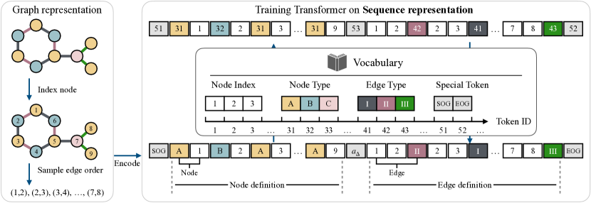
Figure 1: Illustration of our proposed graph sequence representation. This representation can be viewed as a sequence of actions: first generating all nodes (node type, node index), then explicitly adding edges (source node index, destination node index, edge type) step by step until completion. A unified vocabulary is used to map different types of actions into a shared token space.

3.2 Learning Graph Sequences via Transformer

We utilize a transformer decoder (Vaswani, 2017) for modeling the graph sequences. Unlike language models, our defined graph sequence contains tokens from different action spaces. Here we consider using a tokenizer that unifies all types of actions into one vocabulary.

Algorithm 1 Degree-Based Edge Removal Process

  Input: Graph $G=(V,E)$, neighborhood function $\text{Nei}(\cdot)$

  Output: Sequence of removed edges $\sigma_{E}$

  Initialize $\sigma_{E}\leftarrow[~]$

  while $E\neq\emptyset$ do

  Select $v_{\text{src}}\in V$ with the minimum degree.

  Select $v_{\text{dest}}\in\text{Nei}(v_{\text{src}})$ with the minimum degree.

  Remove edge $e=(v_{\text{src}},v_{\text{dest}})$ from $E$; append $e$ to $\sigma_{E}$.

  Update the degrees of $v_{\text{src}}$ and $v_{\text{dest}}$.

  end while

Tokenization.  Let $n_{\text{max}}$ be the maximum number of nodes of a graph dataset. The unified vocabulary lookup is then defined as

$$\text{tokenize}(v^{\text{id}})=v^{\text{id}},~~~v^{\text{id}}\in\{1,\ldots,n_{\text{max}}\};$$

$$\text{tokenize}(v^{c})=v^{c}+n_{\text{max}},~~~v^{c}\in\{1,\ldots,K_{v}\};$$

$$\text{tokenize}(e^{c})=e^{c}+n_{\text{max}}+K_{v},~~~e^{c}\in\{1,\ldots,K_{e}\};$$

$$\text{tokenize}(a_{\Delta})=n_{\text{max}}+K_{v}+K_{e}+1.$$

We additionally introduce special tokens [SOG] and [EOG], representing the start and the end of the sequence generation. We denote the tokenized sequence $\mathbf{s}=[s_{1},\ldots,s_{L}]$, which is used in the following sections.

Training loss.  We use the standard language modeling loss to minimize the negative log-likelihood

$$\mathcal{L}_{\text{pt}}(\theta):=-\log{p_{\theta}(\mathbf{s})}=\sum_{l=1}^{L}\log{p_{\theta}(s_{l}|\mathbf{s}_{<l})},$$

where $\theta$ is the parameters of the model. Since the tokens in sequence are arranged based on the defined rule, the action space for each decoding step is limited to a subset. For example, when the current input token is one of the node type, its output token can only be one of the node indices. One can impose such constraint on the output logits vector at each step to improve the modeling accuracy. In our experiment, we find that an unconstrained logits space can also yield a superior performance due to the expressiveness of transformers.

4 Fine-tuning

After pre-training a model, we further fine-tune it for downstream tasks. We consider generative (§4.1) and predictive (§4.2) downstream tasks, where the former aims to generate graphs with desired properties, and the latter utilizes the graph embeddings learned from the transformer to predict properties.

4.1 Goal-oriented Generation

Let $z(\cdot)$ be the function that estimates property $z$ of a graph $G$. In goal-oriented generation, we are interested in obtaining a new model that generates graphs whose properties are close to $z^{*}$ more often then the pre-trained model. Such a setup has a broad application in the graph generation community such as drug discovery. In this work, we explore obtaining such distribution by fine-tuning the pre-trained model. We consider rejection sampling fine-tuning (RFT) and reinforcement learning (RL) approaches.

Rejection sampling fine-tuning.  This approach fine-tunes the model using its own generated samples that satisfy the desired property $z^{*}$. We consider the case where the property is a scalar, and an acceptance function $m^{z^{*}}_{\omega}(G)=\mathbbm{1}_{|z^{*}-z(G)|<\omega}$ is controlled by an distance threshold $\omega$.

The algorithm for generating the fine-tuning dataset $\mathcal{D}^{y^{*}}_{\omega}=\{G_{b}\}_{b=1}^{B}$ via rejection sampling is shown in Alg. 2. Note that we expect the learned pre-trained model is able to generate graphs with desired property.

When the graph of interest has a low density in the model distribution, RFT becomes inefficient as it rejects most of the samples. To address this, we further propose to self-bootstrap (SBS) the RFT model to approach the target distribution. Specifically, we first define a sequence with $\tau$ thresholds $\omega_{1}>\omega_{2}>\ldots>\omega_{\tau}$, where $\omega_{\tau}=\omega$. Then we can obtained a sequence of fine-tuned models by iteratively constructing fine-tuned datasets using model trained from previous threshold. The SBS algorithm combined with RFT is shown in Alg. 3.

Algorithm 2 RFT Dataset Construction

  Input: Model $p_{\theta}$, acceptance function $m_{\omega}^{z^{*}}$, data size $B$.

  Output: Fine-tuning dataset $\mathcal{D}_{\omega}^{z^{*}}$

  Initialize $\mathcal{D}_{\omega}^{z^{*}}\leftarrow\{~\}$

  while $|\mathcal{D}_{\omega}^{z^{*}}|\neq B$ do

  Generate $G\sim p_{\theta}$.

  if $G$ is valid and $m_{\omega}^{z^{*}}(G)=1$ then

   Append $G$ to $\mathcal{D}_{\omega}^{z^{*}}$.

  end if

  end while

Algorithm 3 SBS^τ combined with RFT

  Input: Model $p_{\theta}$, thresholds list $[\omega_{1}\ldots,\omega_{\tau}]$, data size $B$.

  Output: Fine-tuned model $p_{\theta_{\tau}}$

  Set $\theta_{0}=\theta$.

  for $i=1,\ldots,\tau$ do

  Use $p_{\theta_{i-1}}$ as input model, obtain $\mathcal{D}_{\omega_{i}}^{z^{*}}$ $\leftarrow$ Alg. 2.

  Fine-tune $\theta_{i-1}$ on $\mathcal{D}_{\omega_{i}}^{z^{*}}$, obtain new parameters $\theta_{i}$.

  end for

Reinforcement learning.  Denote a target-relevant reward function $r_{z^{*}}(G)$, we consider a KL-regularized reinforcement learning problem:

$$\phi^{*}=\arg\max_{\phi}\mathbb{E}_{p_{\phi(\mathbf{s})}}\big{[}r_{z^{*}}(\mathbf{s})-\rho_{1}\mathrm{KL}\big{(}p_{\phi}(\cdot|\mathbf{s})\|p_{\theta}(\cdot|\mathbf{s})\big{)}\big{]}.$$

We use the notation $\mathbf{s}$ and $G$ interchangeable as the mapping from $\mathbf{s}$ to $G$ is deterministic. The KL divergence $\mathrm{KL}(\cdot\|\cdot)$ prevents the target model from deviating too much from the pre-trained model.

We choose Proximal Policy Optimization (PPO)  (Schulman et al., 2017) to effectively train the target policy (actor model) without sacrificing stability. We first define the token-level reward:

$$R([\mathbf{s}_{<l},s_{l}])=\begin{cases}0&s_{l}\neq\text{[EOG]}\\ r([\mathbf{s}_{<l},s_{l}])&s_{l}=\text{[EOG]}\\ \end{cases}.$$

Here $\mathbf{s}_{<l}$ is the state of the $l$-th step in a finite trajectory (sequence). We only assign a reward when the generation is completed. The value function of state $\mathbf{s}_{<l}$ under a model $p$ is the expectation of the undiscounted future return:

$$V^{p}(\mathbf{s}_{<l})=\mathbb{E}_{p(\mathbf{s}_{\geq l}|\mathbf{s}_{<l})}\big{[}r({\mathbf{s}})\big{]}.$$

A critic model $V_{\psi}(\mathbf{s}_{<l})$ is then learned to approximate the true value function $V^{p}(\mathbf{s}_{<l})$ via minimizing the mean absolute error $\mathcal{L}_{\text{critic}}(\psi)$. We parameterize the critic model with a transformer that is the same architecture as the pre-trained model, except the logits head is replaced by a value head. The parameters of the critic model are also initialized from the pre-trained model.

We use the clipped surrogate objective $\mathcal{L}_{\text{pg-clip}}(\phi)$ in PPO to optimize the actor model. Moreover, to mitigate possible model degradation, we incorporate the pre-training loss $\mathcal{L}_{\text{pt}}(\phi)$ following Zheng et al. (2023); Liu et al. (2024).

All terms combined, we minimize the objective:

$$\mathcal{L}_{\text{ppo}}(\phi,\psi;\theta)= \mathcal{L}_{\text{pg-clip}}(\phi)+\rho_{2}\mathcal{L}_{\text{critic}}(\psi)+\rho_{3}\mathcal{L}_{\text{pt}}(\phi).$$

Here $\rho_{1},\rho_{2},\rho_{3}$ are loss coefficients. We provide preliminaries of PPO and details of each loss term in Appendix A.

4.2 Property Prediction

Assume a labeled graph dataset $\mathcal{C}$, where each instance consists a graph $G$ along with a label $y$. We fine-tune the pre-trained model on it to learn to predict $y$ given $G$. After the sequence s is generated from $G$, we extract the activation $\mathbf{h}$ of the final token $\mathbf{s}_{L}$ output by the last transformer block as the graph representation. To predict $y$, we then feed $\mathbf{h}$ into a dropout layer followed by a linear layer:

$$p(y|\mathbf{s})=\text{softmax}(\text{Dropout}(\text{Linear}(\mathbf{h}))).$$

We then maximize the log-likelihood $\mathbb{E}_{(G,y)\sim\mathcal{C}}\log p(y|G)$. Compared to freezing the whole transformer during training and only update parameters of the linear layer, we found that unlocking the latter half of the transformer blocks significantly enhances performance.

Model	Planar						Tree
	Deg.$\downarrow$	Clus.$\downarrow$	Orbit$\downarrow$	Spec.$\downarrow$	Wavelet$\downarrow$​​​	​​​V.U.N.$\uparrow$	Deg.$\downarrow$	Clus.$\downarrow$	Orbit$\downarrow$	Spec.$\downarrow$	Wavelet$\downarrow$​​​	​​​V.U.N.$\uparrow$
GRAN (Liao et al., 2019)	7e-4	4.3e-2	9e-4	7.5e-3	1.9e-3	0	1.9e-1	8e-3	2e-2	2.8e-1	3.3e-1	0
BiGG (Dai et al., 2020)	7e-4	5.7e-2	3.7e-2	1.1e-2	5.2e-3	5	1.4e-3	0.00	0.00	1.2e-2	5.8e-3	75
DiGress (Vignac et al., 2022)	7e-4	7.8e-2	7.9e-3	9.8e-3	3.1e-3	77.5	2e-4	0.00	0.00	1.1e-2	4.3e-3	90
BwR (Diamant et al., 2023)	2.3e-2	2.6e-1	5.5e-1	4.4e-2	1.3e-1	0	1.6e-3	1.2e-1	3e-4	4.8e-2	3.9e-2	0
HSpectre (Bergmeister et al., 2023)​​​	5e-4	6.3e-2	1.7e-3	7.5e-3	1.3e-3	95	1e-4	0.00	0.00	1.2e-2	4.7e-3	100
DeFoG (Qin et al., 2024)	5e-4	5e-2	6e-4	7.2e-3	1.4e-3	99.5	2e-4	0.00	0.00	1.1e-2	4.6e-3	96.5
G2PT${}_{\text{small}}$	4.7e-3	2.4e-3	0.00	1.6e-2	1.4e-2	95	2e-3	0.00	0.00	7.4e-3	3.9e-3	99
G2PT${}_{\text{base}}$	1.8e-3	4.7e-3	0.00	8.1e-3	5.1e-3	100	4.3e-3	0.00	1e-4	7.3e-3	5.7e-3	99
Model	Lobster						SBM
	Deg.$\downarrow$	Clus.$\downarrow$	Orbit$\downarrow$	Spec.$\downarrow$	Wavelet$\downarrow$​​​	​​​V.U.N.$\uparrow$	Deg.$\downarrow$	Clus.$\downarrow$	Orbit$\downarrow$	Spec.$\downarrow$	Wavelet$\downarrow$​​​	​​​V.U.N.$\uparrow$
GRAN (Liao et al., 2019)	3.8e-2	0.00	1e-3	2.7e-2	-	-	1.1e-2	5.5e-2	5.4e-2	5.4e-3	2.1e-2	25
BiGG (Dai et al., 2020)	0.00	0.00	0.00	9e-3	-	-	1.2e-3	6.0e-2	6.7e-2	5.9e-3	3.7e-2	10
DiGress (Vignac et al., 2022)	2.1e-2	0.00	4e-3	-	-	-	1.8e-3	4.9e-2	4.2e-2	4.5e-3	1.4e-3	60
BwR (Diamant et al., 2023)	3.2e-1	0.00	2.5e-1	-	-	-	4.8e-2	6.4e-2	1.1e-1	1.7e-2	8.9e-2	7.5
HSpectre (Bergmeister et al., 2023)​​​	​​​-	-	-	-	-	-	1.2e-2	5.2e-2	6.7e-2	6.7e-3	2.2e-2	45
DeFoG (Qin et al., 2024)	-	-	-	-	-	-	6e-4	5.2e-2	5.6e-2	5.4e-3	8e-3	90
G2PT${}_{\text{small}}$	2e-3	0.00	0.00	5e-3	8.5e-3	100	3.5e-3	1.2e-2	7e-4	7.6e-3	9.8e-3	100
G2PT${}_{\text{base}}$	1e-3	0.00	0.00	4e-3	1e-2	100	4.2e-3	5.3e-3	3e-4	6.1e-3	6.9e-3	100

Table 2: Generative performance on generic graph datasets.

5 Experiments

5.1 Setup

Datasets.  We consider both generative tasks and predictive tasks in our experiments. In generative tasks, we consider training transformer decoders on molecular datasets and generic graph datasets. For molecular datasets, we use QM9 (Wu et al., 2018b), MOSES (Polykovskiy et al., 2020), and GuacaMol (Brown et al., 2019). For generic graph datasets, we adapted the widely used datasets: Planar, Tree, Lobster, and stochastic block model (SBM). In predictive tasks, we fine-tune models pre-trained from GuacaMol datasets on various molecular property tasks using MoleculeNet (Wu et al., 2018a), detailed in Section B.4, to verify the usefulness of the learned graph representations.

Model specifications.  We train transformers with three different sizes: (1) the small transformer has 6 transformer layers and 6 attention head, with $d_{\text{model}}=384$, leading to approximately 10M parameters; (2) the base transformer has 12 transformer layers and 12 attention head, with $d_{\text{model}}=768$, leading to approximately 85M parameters; (2) the large transformer has 24 transformer layers and 16 attention head, with $d_{\text{model}}=1024$, leading to approximately 300M parameters. We use different specifications for different experiments according to the task complexity.

5.2 A Demonstrative Experiment using Planar Graphs

We first validate the effectiveness of our proposed graph sequence representation compared to the adjacency matrix. To achieve this, we train transformer decoders on planar graphs using both representations and evaluate their generative performance. For the adjacency representation, planar graphs are encoded as sequences of 0s and 1s derived from the strictly lower triangular matrix, with rows and columns permuted using BFS orderings to augment the training dataset. Table 3 presents the quantitative and qualitative results of the generated samples. Our proposed representation demonstrates superior generative performance with a much smaller set of tokens, while model learning adjacency matrices struggles to capture the topological rules of the training graphs.

5.3 Generic Graph Generation

We evaluate G2PT on four generic datasets using Maximum Mean Discrepancy (MMD) to compare the graph statistics distributions of generated and test graphs. The evaluation considers degree (Deg.), clustering coefficient (Clus.), orbit counts (Orbit), spectral properties (Spec.), and wavelet statistics. Moreover, we report the percentage of valid, unique, and novel samples (V.U.N.) (Vignac et al., 2022). For this task, we trained the G2PT${}_{\text{small}}$ and G2PT${}_{\text{base}}$ models.

As shown in Table 2, G2PT demonstrates superior performance compared to the baselines. The details about baseline and metric are introduced in appendix B.5 The base model achieves 11 out of 24 best scores and ranks in the top two for 17 out of 24 metrics. The small model also demonstrates competitive results, indicating that a lightweight model can effectively capture the graph patterns in the datasets.

Rep.​​​	​​​#Tokens$\downarrow$​​​	​​​Deg.$\downarrow$​​​	​​​Clus.$\downarrow$​​​	​​​Orbit$\downarrow$​​​	​​​Spec.$\downarrow$​​​	​​​Wavelet$\downarrow$​​​	​​​V.U.N.$\uparrow$
$\mathbf{A}$	2018	8.6e-3	1e-1	8e-3	3.2e-2	6.1e-2	94
Ours	737	4.7e-3	2.4e-3	0.00	1.6e-2	1.4e-2	95

$\mathbf{A}$		Ours
​​​​​​​​​​​​​​​​	​​​​​​​​ ​​​​​	​​​​​ ​​​​​​​​	​​​​​​​​ ​​​​​​​​

Table 3: Generative performance comparison between the proposed edge sequence and adjacency matrix representations.

Model	MOSES							GuacaMol
	Validity$\uparrow$​​	​​Unique.$\uparrow$​​	​​Novelty$\uparrow$​​	​​Filters$\uparrow$​​	​​FCD$\downarrow$​​	​​SNN$\uparrow$​​	Scaf$\uparrow$	Validity$\uparrow$​​	​​Unique.$\uparrow$​​	​​Novelty$\uparrow$​​	​​KL Div.$\uparrow$​​	FCD$\uparrow$
DiGress (Vignac et al., 2022)​​​​	85.7	100	95.0	97.1	1.19	0.52	14.8	85.2	100	99.9	92.9	68
DisCo (Xu et al., 2024)​​​​	88.3	100	97.7	95.6	1.44	0.5	15.1	86.6	86.6	86.5	92.6	59.7
Cometh (Siraudin et al., 2024)​​​​	90.5	99.9	92.6	99.1	1.27	0.54	16.0	98.9	98.9	97.6	96.7	72.7
DeFoG (Qin et al., 2024)​​​​	92.8	99.9	92.1	99.9	1.95	0.55	14.4	99.0	99.0	97.9	97.9	73.8
G2PT${}_{\text{small}}$	95.1	100	91.7	97.4	1.10	0.52	5.0	90.4	100	99.8	92.8	86.6
G2PT${}_{\text{base}}$	96.4	100	86.0	98.3	0.97	0.55	3.3	94.6	100	99.5	96.0	93.4
G2PT${}_{\text{large}}$	97.2	100	79.4	98.9	1.02	0.55	2.9	95.3	100	99.5	95.6	92.7

Model	QM9
	​Validity$\uparrow$​	​​​​Unique.$\uparrow$​​​​	​​​​FCD$\downarrow$​​​​
DiGress (Vignac et al., 2022)​​​	99.0	96.2	-
DisCo (Xu et al., 2024)​​​	99.6	96.2	0.25
Cometh (Siraudin et al., 2024)​​​	99.2	96.7	0.11
DeFoG (Qin et al., 2024)​​​	99.3	96.3	0.12
G2PT${}_{\text{small}}$	99.0	96.7	0.06
G2PT${}_{\text{base}}$	99.0	96.8	0.06
G2PT${}_{\text{large}}$	98.9	96.7	0.06

MOSES			GuacaMol
Train	G2PT${}_{\text{small}}$	G2PT${}_{\text{base}}$	Train	G2PT${}_{\text{small}}$	G2PT${}_{\text{base}}$
​​	​​​​	​​	​​	​​​​	​​
​​	​​​​	​​	​​	​​​​	​​

Table 4: Generative performance on molecular graph datasets

Density ​​​​​​​​​	​​​​​​​​​​​​​​	​​​​​ ​​​​​	​​​​​
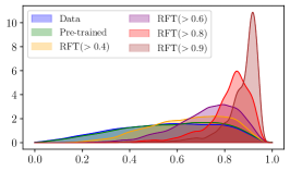
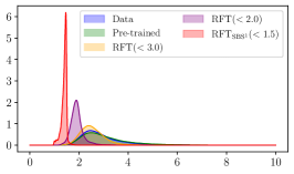
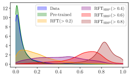
	QED Score	SA Score	GSK3$\beta$ Score
(a) Rejection sampling fine-tuning (with self-bootstrap)
Density ​​​​​​​​​	​​​​​​​​​​​​​​	​​​​​ ​​​​​	​​​​​
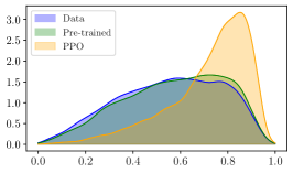
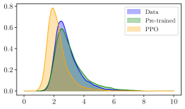
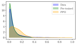
	QED Score	SA Score	GSK3$\beta$ Score
(b) Reinforcement learning framework (PPO)

Figure 2: Goal-oriented molecule generation using QED, SA and GSK3$\beta$ scores. Top row (a) shows the results using RFT, and bottom row (b) shows the results using RL.

5.4 Molecule Generation

De novo molecular design is a key real-world application of graph generation. We assess G2PT’s performance on the QM9, MOSES, and GuacaMol datasets. For the QM9 dataset, we adopt the evaluation protocol in Vignac et al. (2022). For MOSES and GuacaMol, we utilize the evaluation pipelines provided by their respective toolkits (Polykovskiy et al., 2020; Brown et al., 2019).

The quantitative results are presented in Table 4. On MOSES, G2PT surpasses other state-of-the-art models in validity, uniqueness, FCD, and SNN metrics. We introduce the details for metrics in appendix B.6. Notably, the FCD, SNN, and scaffold similarity (Scaf) evaluations compare generated samples to a held-out test set, where the test molecules have scaffolds distinct from the training data. Although the scaffold similarity score is relatively low, the overall performance indicates that G2PT achieves a better goodness of fit on the training set. G2PT also delivers strong performance on the GuacaMol and QM9 datasets. We additionally provide qualitative examples from the MOSES and GuacaMol datasets in the table.

	BBBP	Tox21	ToxCast	SIDER	ClinTox	MUV	HIV	BACE	Avg.
AttrMask (Hu et al., 2020)	70.2$\pm$0.5	74.2$\pm$0.8	62.5$\pm$0.4	60.4$\pm$0.6	68.6$\pm$9.6	73.9$\pm$1.3	74.3$\pm$1.3	77.2$\pm$1.4	70.2
InfoGraph (Sun et al., 2020)	69.2$\pm$0.8	73.0$\pm$0.7	62.0$\pm$0.3	59.2$\pm$0.2	75.1$\pm$5.0	74.0$\pm$1.5	74.5$\pm$1.8	73.9$\pm$2.5	70.1
ContextPred (Hu et al., 2020)	71.2$\pm$0.9	73.3$\pm$0.5	62.8$\pm$0.3	59.3$\pm$1.4	73.7$\pm$4.0	72.5$\pm$2.2	75.8$\pm$1.1	78.6$\pm$1.4	70.9
GraphCL (You et al., 2021)	67.5$\pm$2.5	75.0$\pm$0.5	62.8$\pm$0.2	60.1$\pm$1.3	78.9$\pm$4.2	77.1$\pm$1.0	75.0$\pm$0.4	68.7$\pm$7.8	70.6
GraphMVP (Liu et al., 2022a)	68.5$\pm$0.2	74.5$\pm$0.0	62.7$\pm$0.1	62.3$\pm$1.6	79.0$\pm$2.5	75.0$\pm$1.4	74.8$\pm$1.4	76.8$\pm$1.1	71.7
GraphMAE (Hou et al., 2022b)	70.9$\pm$0.9	75.0$\pm$0.4	64.1$\pm$0.1	59.9$\pm$0.5	81.5$\pm$2.8	76.9$\pm$2.6	76.7$\pm$0.9	81.4$\pm$1.4	73.3
G2PT${}_{\text{small}}$ (No pre-training)	60.7$\pm$0.3	66.4$\pm$0.5	57.0$\pm$0.3	61.6$\pm$0.2	67.8$\pm$1.1	45.8$\pm$8.5	70.1$\pm$7.5	68.8$\pm$1.3	62.3
G2PT${}_{\text{base}}$ (No pre-training)	56.5$\pm$0.2	67.4$\pm$0.4	57.9$\pm$0.1	60.2$\pm$2.8	71.0$\pm$5.6	60.1$\pm$1.3	72.7$\pm$1.1	73.4$\pm$0.3	64.9
G2PT${}_{\text{small}}$	68.5$\pm$0.5	74.7$\pm$0.2	61.2$\pm$0.1	61.7$\pm$1.0	82.3$\pm$2.2	74.9$\pm$0.1	75.7$\pm$0.4	81.3$\pm$0.5	72.5
G2PT${}_{\text{base}}$	71.0$\pm$0.4	75.0$\pm$0.3	63.0$\pm$0.5	61.9$\pm$0.2	82.1$\pm$1.1	74.5$\pm$0.3	76.3$\pm$0.4	82.3$\pm$1.6	73.3

Table 5: Results for molecule property prediction in terms of ROC-AUC. We report mean and standard deviation over three runs.

5.5 Goal-oriented Generation

In addition to distribution learning which aims to draw independent samples from the learned graph distribution, goal-oriented generation is a major task in graph generation that aims to draw samples with additional constraints or preferences and is key to many applications such as molecule optimization (Du et al., 2024).

We validate the capability of G2PT on goal-oriented gen- eration by fine-tuning the pre-trained model. Practically, we employ the model pre-trained on GuacaMol dataset and select three commonly used physiochemical and binding-related properties: quantitative evaluation of druglikeness (QED), synthesis accessibility (SA), and the activity against target protein Glycogen synthase kinase 3 beta (GSK3$\beta$), detailed in Appendix B.3. The property oracle functions are provided by the Therapeutics Data Commons (TDC) package (Huang et al., 2022).

As discussed in §4.1, we employ two approaches for fine-tuning: (1) rejection sampling fine-tuning and (2) reinforcement learning with PPO. Figure 2 shows that both methods can effectively push the learned distribution to the distribution of interest. Notably, RFT, with up to three rounds of SBS, significantly shifts the distribution towards a desired one. In contrast, PPO, despite biasing the distribution, suffers from the over-regularization from the base policy, which aims for training stability. In the most challenging case (GSK3$\beta$), PPO fails to sampling data with high rewards. Conversely, RFT overcomes the barrier in the second round (RFT${}_{\text{SBS}^{1}}$), where its distribution becomes flat across the range and quickly transitions to a high-reward distribution.

5.6 Predictive Performance on Downstream Tasks

We conduct experiments on eight graph classification benchmark datasets from MoleculeNet (Wu et al., 2018a), strictly following the data splitting protocol used in GraphMAE (Hou et al., 2022a) for fair comparison. A detailed description of these datasets is provided in Appendix B.4.

For downstream fine-tuning, we initialize G2PT with parameters pre-trained on the GuacaMol dataset, which contains molecules with up to 89 heavy atoms. We also provide results where models are not pre-trained.

As summarized in Table 5, G2PT’s graph embeddings demonstrate consistently strong (best or second-best) performance on seven out of eight downstream tasks, achieving an overall performance comparable to GraphMAE, a leading self-supervised learning (SSL) method. Notably, while previous SSL approaches leverage additional features such as 3D information or chirality, G2PT is trained exclusively on 2D graph structural information. Overall, these results indicate that G2PT not only excels in generation but also learns effective graph representations.

5.7 Scaling Effects

We analyze how scaling the model size and data size will affect the model performance using the three molecular datasets. We use the validity score to quantify the model performance. Results are provided in Figure 3.

For model scaling, we additionally train G2PTs with 1M, 705M, and 1.5B parameters. We notice that as model size increases, validity score generally increases and saturates at some point, depending on the task complexity. For instance, QM9 saturates at the beginning (1M parameters) while MOSES and GuacaMol require more than 85M (base) parameters to achieve satisfying performance.

For data scaling, we generating multiple sequences from the same graph to improve the diversity of the training data. The number of augmentation per graph is chosen from $\{1,10,100\}$. As shown, one sequence per graph is insufficient to train transformers effectively, and improving data diversity helps improve model performance. Similar to model scaling, performance saturated at some point when enough data are used.

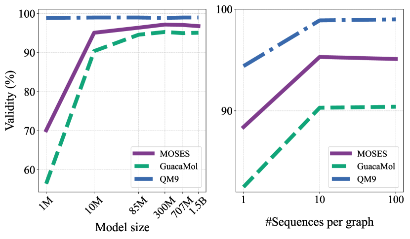
Figure 3: Model and data scaling effects.

6 Conclusion

This work revisits the graph generative models and proposes a novel sequence-based representation that efficiently encodes graph structures via node and edge definitions. This representation serves as the foundation for the proposed Graph Generative Pre-trained Transformer (G2PT), an auto-regressive model that effectively models graph sequences using next-token prediction. Extensive evaluations demonstrated that G2PT achieves remarkable performance across multiple datasets and tasks, including generic graph and molecule generation, as well as downstream tasks like goal-oriented graph generation and graph property prediction. The results highlight G2PT’s adaptability and scalability, making it a versatile framework for various applications. One limitation of our method is that G2PT is order-sensitive, where different graph domains may prefer different edge orderings. Future research could be done by exploring edge orderings that are more universal and expressive.

Appendix A Reinforcement Learning Details

A.1 Preliminaries on Proximal Policy Optimization (PPO)

Generalized Advantage Estimation.

In reinforcement learning, the Q function $Q(\mathbf{s}_{<l},s_{l})$ captures the expected returns when taking an action $s_{l}$ at current state $\mathbf{s}_{<l}$, and the value function $V(\mathbf{s}_{<l})$ captures the expected return following the policy from a given state $\mathbf{s}_{<l}$.

The advantage function $A(s_{l},\mathbf{s}_{<l})$, defined as the difference between the Q function and the value function, measures whether taking action $s_{l}$ is better or worse than the policy’s default behavior. In practice, the Q function is estimated using the actual rewards $r_{l}$ and the estimated future returns (the value function). There are two commonly used estimators, one is the one-step Temporal Difference (TD):

$$\hat{Q}(\mathbf{s}_{<l},s_{l}) =r_{l}+\gamma V(\mathbf{s}_{<l+1}),$$

$$\hat{A}(\mathbf{s}_{<l},s_{l}) =r_{l}+\gamma V(\mathbf{s}_{<l+1})-V(\mathbf{s}_{<l}),$$

and the full Monte Carlo (MC):

$$\hat{Q}(\mathbf{s}_{<l},s_{l}) =\sum_{l^{\prime}=l}^{L}\gamma^{l^{\prime}-l}r_{l^{\prime}},$$

$$\hat{A}(\mathbf{s}_{<l},s_{l}) =\sum_{l^{\prime}=l}^{L}\gamma^{l^{\prime}-l}r_{l^{\prime}}-V(\mathbf{s}_{<l}),$$

assuming finite trajectory with $L$ steps in total. However, the TD estimator exhibits high bias and the MC estimator exhibits high variance. The Generalized Advantage Estimation (GAE) (Schulman et al., 2015) effectively balances the high bias and high variance smoothly using a trade-off parameter $\gamma$. Let $\delta_{l}=r_{t}+\gamma V(\mathbf{s}_{<l+1})-V(\mathbf{s}_{<l})$, the definition of GAE is:

$$\hat{A}^{\gamma}(\mathbf{s}_{<l},s_{l}) =\sum_{l^{\prime}=l}^{L}(\gamma\lambda)^{l^{\prime}-l}\delta_{l^{\prime}}=\delta_{l}+\hat{A}^{\gamma}(\mathbf{s}_{<l+1},s_{l+1}).$$

GAE plays an important role in estimating the policy gradient, and will be used in the PPO algorithm.

Proximal Policy Optimization.

PPO (Schulman et al., 2017) is a fundamental technique in reinforcement learning, designed to train policies efficiently while preserving stability. It is built on the principle that gradually guides the policy towards an optimal solution, rather than applying aggressive updates that could compromise the stability of the learning process.

In traditional policy gradient methods, the new policy should remain close to the old policy in the parameters space. However, proximity in parameter space does not indicate similar performance. A large update step in policy may lead to falling “off the cliff”, thus getting a bad policy. Once it is stuck in a bad policy, it will take a very long time to recover.

PPO introduces two kinds of constraints on policy updates. The first kind is to add an KL-regularization term to the policy gradient “surrogate” objective

$$\mathcal{L}_{\text{pg-penalty}}(\phi)=\hat{\mathbb{E}}_{l}\bigg{[}\frac{p_{\phi}(s_{l}|\mathbf{s}_{<l})}{p_{\phi_{\text{old}}}(s_{l}|\mathbf{s}_{<l})}\hat{A}_{l}\bigg{]}-\beta\mathrm{KL}(p_{\phi_{\text{old}}}(\cdot|\mathbf{s}_{<l})\|p_{\phi}(\cdot|\mathbf{s}_{<l})).$$

Here $\hat{\mathbb{E}}_{l}[\cdot]$ is the empirical average over a finite batch of samples where sampling and optimization alternates. $\beta$ is the penalty factor. $\hat{A}_{l}:=\hat{A}^{\gamma}(\mathbf{s}_{<l},s_{l})$ is GAE, which is detailed in last section.

The second type is the clipped surrogate objective, expressed as

$$\mathcal{L}_{\text{pg-clip}}(\phi)=\hat{\mathbb{E}}_{l}\bigg{[}\min\bigg{(}\frac{p_{\phi}(s_{l}|\mathbf{s}_{<l})}{p_{\phi_{\text{old}}}(s_{l}|\mathbf{s}_{<l})}\hat{A}_{l},\text{clip}\bigg{(}\frac{p_{\phi}(s_{l}|\mathbf{s}_{<l})}{p_{\phi_{\text{old}}}(s_{l}|\mathbf{s}_{<l})},1-\epsilon,1+\epsilon\bigg{)}\hat{A}_{l}\bigg{)}\bigg{]},$$

where $\frac{p_{\phi}(s_{l}|\mathbf{s}_{<l})}{p_{\phi_{\text{old}}}(s_{l}|\mathbf{s}_{<l})}$ is the probability ratio between the new and the old policy. And $\epsilon$ decides how much the new policy can deviate from the one policy. The clipping operations prevent the policy from changing too much from the older one within one iteration. In the following, we elaborate on how the critic model is optimized.

Value Function Approximation.

The critic model $V_{\psi}(\mathbf{s}_{<l})$ in PPO algorithm is used to approximate the actual value function $V^{p}(\mathbf{s}_{<l})$. We use the mean absolute value loss to minimize the difference between the predicted values and the actual return values. Specifically, the objective is

$$\mathcal{L}_{\text{critic}}=\hat{\mathbb{E}}_{l}\big{[}|V_{\psi}(\mathbf{s}_{<l})-\hat{V}(\mathbf{s}_{<l})|\big{]}.$$

Here the actual return value is estimated using GAE to balance the bias and variance:

$$\hat{V}(\mathbf{s}_{<l})=\hat{A}(\mathbf{s}_{<l},s_{l})+V_{\psi_{\text{old}}}(\mathbf{s}_{<l}),$$

where $V_{\psi_{\text{old}}}(\mathbf{s}_{<l})$ is collected during the sampling step in PPO. The critic loss is weight by a factor $\rho_{2}$.

A.2 KL-regularization

As mentioned in §4.1, we adopt a KL-regularized reinforcement learning approach. Unlike the KL penalty in $\mathcal{L}_{\text{pg-penalty}}(\phi)$, this regularizer ensures that the policy model $p_{\phi}$ does not diverge significantly from the reference model $p_{\theta}$. Instead of optimizing this term directly, we incorporate it into the rewards $r_{l}$. Specifically, we define:

$$r^{\rho_{1}}_{l}=r_{l}-\rho_{1}\mathrm{KL}(p_{\phi}(\cdot|[\mathbf{s}_{<l},s_{l}])\|p_{\theta}(\cdot|[\mathbf{s}_{<l},s_{l}])),$$

where $\rho_{1}$ is the penalty factor. In practice, $\rho_{1}$ is set to a small value, such as 0.03, to promote exploration.

	QM9	MOSES	GuacaMol	Planar	Tree	Lobster	SBM
#Node Types	4	8	12	1	1	1	1
#Edge Types	4	4	4	1	1	1	1
Avg. #Nodes	8.79	21.67	27.83	64	64	55	104.01
Min. #Nodes	1	8	2	64	64	10	44
Max. #Nodes	9	27	88	64	64	100	187
#Training Sequences	9,773,200	141,951,200	111,863,300	12,800,000	10,000,000	12,800,000	12,800,000
Vocabulary Size	27	60	120	73	73	110	195
Max Sequence Length	85	207	614	737	383	599	3950

Table 6: Dataset statistics.

A.3 Pre-training loss

Following Zheng et al. (2023) and Liu et al. (2024), we incorporate the pre-training loss $\mathcal{L}_{\text{pt}}(\phi)$ o mitigate potential degeneration in the model’s ability to produce valid sequences. This is particularly beneficial for helping the actor model recover when it “falls off the grid” during PPO. The pre-training data is sourced from the dataset used to train the reference model, and the loss $\mathcal{L}_{\text{pt}}(\phi)$ is weighted by the coefficient $\rho_{3}$.

Appendix B Additional Experimental Details

B.1 Graph Generative Pre-training

Generative pre-training leverages graph-structured data to learn foundational representations that can be fine-tuned for downstream tasks.

Sequence conversion.

We convert graphs into sequences of tokens that represent nodes and edges. This transformation involves encoding the molecular structure in a sequential format that captures both the composition and the order of assembly. For instance, we iteratively process the nodes and edges, and insert special tokens to mark key points in the sequence, such as the start and end of generation. Additionally, we apply preprocessing steps like filtering molecules by size, removing hydrogens, or addressing dataset-specific constraints to ensure consistency and suitability for the target tasks.

Data splitting.

We divide generic datasets into training, validation, and test sets based on splitting ratios 6:2:2. For the molecular datasets, we follow the default settings of the datasets.

Dataset statistics.

The vocabulary size, maximum sequence length, and other parameters vary across datasets due to their distinct molecular characteristics. We summarize the specifications in Table 6, which includes details on the number of node types, edge types, and graphs for each dataset.

Hyperparameters.

Table 7 provides hyperparameters used for training three distinct model sizes, corresponding to approximately 10M, 85M, and 300M parameters, respectively.

	10M	85M	300M
Architecture
#layers	6	12	24
#heads	6	12	16
$d_{\text{model}}$	384	768	1024
dropout rate	0.0
Training
Lr	1e-4
Optimizer	AdamW (Loshchilov & Hutter, 2019)
Lr scheduler	Cosine
Weight decay	1e-1
#iterations	300000
Batch size	60	60	30
#Gradient Accumulation	8	8	16
Grad Clipping Value	1
#Warmup Iterations	2000

Table 7: Hyperparameters for graph generative pre-training.

B.2 Demonstration Experiment

We elaborate on how to represent adjacency matrix as sequence and train a transformer decoder on it. We choose planar graphs as the investigation object as it requires a model to be able to capture the rule embedded in the graph. We use G2PT${}_{\text{small}}$ for this experiment.

Sequence conversion.

We convert a 2-D adjacency matrix into a 1-D sequence before training the models. Similar to GraphRNN (You et al., 2018b), we consider modeling the strictly lower triangle of the adjacency matrix. To obtain sequence, we flatten the triangle by concatenating the rows together. The $i$-th row has $i-1$ entries, where each entry is either 0 or 1. We employ BFS to determine the node orderings, which is used to permute the rows and columns of the adjacency matrix to reduce the learning complexity (as uniform orderings are generally harder to fit (Chen et al., 2021)).

	QED	SA	GSK3$\beta$
$\gamma$	1.0
$\lambda$	1.0
$\rho_{1}$	0.5
$\rho_{2}$	0.03	0.03	0.05
$\rho_{3}$	0.03
Advantage Normalization and Clipping	Yes	No	No
Reward Normalization and Clipping	No	Yes	Yes
Ratio Clipping ($\epsilon$)	[0.2]
Critic Value Clipping	[0.2]
Entropy Regularization	No
Gradient Clipping Value	1.0
Actor Lr	1.0
Critic Lr	0.5	0.5	1.0
#Iterations	6000
Batch size	60

Table 8: Hyperparameters used for PPO training.

Training transformers on adjacency matrices.

After obtaining the sequence representation, we prepend and append two special tokens, [SOG] and [EOG], to mark the start and end of the generation of each sequence. The sequence is then tokenized using a vocabulary of size 4, and the transformer is trained on these sequences. Note that no additional token is needed to indicate transitions between rows, as the flattened sequence maintains a fixed correspondence between positions and the referenced node pairs. Specifically, the original row and column indices in the adjacency matrix for the $i$-th entry in the sequence can be determined as:

$$\text{row}=\left\lceil{\frac{1+\sqrt{1+8i}}{2}}\right\rceil,\text{col}=i-\frac{(\text{row}-1)(\text{row}-2)}{2}.$$

Here $\left\lceil\cdot\right\rceil$ is the ceiling operation. Such correspondence is agnostic to graph size and can be inferred by transformers by using positional embeddings.

B.3 Fine-tuning G2PT for Goal-oriented Generation

For the goal-oriented generation, we fine-tune G2PT to generate molecules with desired characteristics. Specifically, we consider three properties that are commonly used for molecule optimization whose functions are easily accessed through the Therapeutics Data Commons (TDC) package (Huang et al., 2022).

• Quantitative evaluation of druglikeness (QED): range 0-1, the higher the more druglike.

• Synthesis accessibility (SA) score: range 1-10, the lower the more synthesizable.

• GSK3$\beta$: activity against target protein Glycogen synthase kinase 3 beta, range 0-1, the higher the better activity.

We use the 85M model pre-trained on GucaMol dataset for all experiments. Below we elaborate on how the RFT and RL algorithms implement each optimization task (property).

Rejection-sampling fine-tuning.

For RFT algorithm without SBS, we begin by generating samples using the pre-trained model and retain only those that meet the criteria defined by the acceptance function $m_{\omega}^{z^{*}}(\cdot)$. We collect 200,000 qualified samples from the generations. Then, we fine-tune the model by initializing it with pre-trained parameters. When combining RFT with SBS, we repeat this process iteratively, using the fine-tuned model from the previous iteration for both sampling and parameter initialization.

For QED score, we retain samples with scores exceeding thresholds of 0.4, 0.6, 0.8, or 0.9. We do not use the SBS algorithm here, as the pre-trained model generates samples efficiently across all QED score ranges.

For SA score, we consider thresholds of $\{<3.0,<2.0,<1.5\}$. We find that the pre-trained model efficiently generates molecules with SA scores below 2.0 and 3.0 but struggles with scores below 1.5. To address this, we bootstrap the fine-tuned model from the 2.0 threshold to the 1.5 threshold.

For GSK3$\beta$, we consider thresholds in $\{>0.2,>0.4,>0.6,>0.8\}$. We observe that the pre-trained model’s score distribution is skewed towards 0, making it challenging to generate satisfactory samples. To resolve this, we fine-tune the model at the 0.2 threshold and progressively bootstrap it through intermediate thresholds (0.4, 0.6) up to 0.8, performing three bootstrapping steps in total.

All models are trained for 6000 iterations, with batch size of 120 and learning rate of 1e-5. The learning rate gradually decay to 0 using Cosine scheduler.

Reinforcement learning.

We use the PPO algorithm to further optimize the pre-trained model. In practice, the token-level reward $R([\mathbf{s}_{<l},s_{l}])$ is set to 0 except when $s_{l}=\text{[EOG]}$. The final reward $r(\mathbf{s})$ for the three properties are designed as follow:

$$r^{\text{QED}}(\mathbf{s}) =\mathbbm{1}_{s\rightarrow G}\max(0.2,2\times(\text{QED}(G)-0.5)),$$ (1)

$$r^{\text{SA}}(\mathbf{s}) =\mathbbm{1}_{s\rightarrow G}\max(0.2,0.2\times(5-\text{SA}(G)),$$ (2)

$$r^{\text{GSK3}\beta}(\mathbf{s}) =\mathbbm{1}_{s\rightarrow G}(5\times(\text{GSK3}\beta(G)).$$ (3)

The indicator function $\mathbbm{1}_{s\rightarrow G}$ assigns 0 to the final reward when the generated sequence $\mathbf{s}$ is invalid. We show the PPO hyperparameters for each targeted task in Table 8.

B.4 Fine-tuning G2PT for Graph Property Prediction

Datasets.

We use eight classification tasks in MoleculeNet (Wu et al., 2018a) following Zhu et al. (2024) to validate the predictive capability of our learned representations.

The datasets cover two types of molecular properties: biophysical and physiological properties.

• Biophysical properties include (1) the HIV dataset for HIV replication inhibition, (2) the Maximum Unbiased Validation (MUV) dataset for virtual screening with nearst neighbor search, (3) the BACE dataset for inhibition of human $\beta$-secretase 1 (BACE-1), and (4) the Side Effect Resource (SIDER) dataset for grouping the side effects of marketed drugs into 27 system organ classes.

• Physiological properties include (1) the Blood-brain barrier penetration (BBBP) dataset for predicting barrier permeability of molecules targeting central nervous system, (2) the Tox21, (3) the ClinTox, and (4) the ToxCast datasets that are all associated with certain type of toxicity of the chemical compounds.

We adopt the scaffold split that divides train, validation and test set by different scaffolds, introduced by Wu et al. (2018b).

Fine-tuning details.

We fine-tune G2PT${}_{\text{small}}$ and G2PT${}_{\text{base}}$ pre-trained on GuacaMol dataset for the downstream tasks. We setup the dropout rate to 0.5 and use a learning rate of 1e-4 for training the linear layer. For the half transformer blocks, we use a learning rate of 1e-6. We use a batch size of 256 and train the models for 100 epochs. Test result with best validation performance is reported.

B.5 Baselines

We evaluate our proposed method against a variety of baselines across different datasets. The baselines include models that span diverse methodologies, ranging from graph neural networks to transformer-based architectures.

Generic graph datasets. The performance of baseline models on Planar, Tree, Lobster, and SBM datasets is shown in Table 2. We consider baselines mainly from two categories: auto-regressive and diffusion graph models. Among them, GRAN (Liao et al., 2019), BiGG (Dai et al., 2020), and BwR (Diamant et al., 2023) are auto-regressive models that sequentially generate graphs. GRAN uses attention-based GNNs to perform block-wise generation, focusing on dependencies between components within the graph. In contrast, BiGG addresses the challenges of efficiency by leveraging the sparsity of real-world graphs to avoid constructing dense representations. Unlike GRAN and BiGG, BwR simplifies the generation process further by restricting graph bandwidth. On the other hand, DiGress (Vignac et al., 2022) and HSpectra (Bergmeister et al., 2023) are built based on diffusion frameworks. DiGress is the first approach that uses a discrete diffusion model to iteratively modify graphs, while HSpectra focuses on multi-scale graph construction by progressively generating graphs through localized denoising diffusion.

Molecule generation datasets. We compare G2PT against four baselines: DiGress (Vignac et al., 2022), DisCo (Xu et al., 2024), Cometh (Siraudin et al., 2024), and DeFoG (Qin et al., 2024). Among them, DisCo and Cometh are both based on a continuous-time discrete diffusion framework, with Cometh additionally incorporating positional encoding for nodes and separate noising processes for nodes and edges. DeFoG adopts a discrete flow matching approach with a linear interpolation noising process.

Graph pre-training methods. We compare against several pre-training approaches for molecular property prediction, as summarized in Table 5. The goal ofGraph pre-training methods is to learn robust graph representations via exploiting the structural information. AttrMask (Hu et al., 2020) uses attribute masking at both node and graph levels to capture local and global features simultaneously. ContextPred (Hu et al., 2020) builds on this idea by predicting subgraph contexts, enabling the model to understand patterns beyond individual attributes. Similarly, InfoGraph (Sun et al., 2020) focuses on multi-scale graph representations by maximizing mutual information between graph-level embeddings and substructures. Moving to contrastive learning approaches, GraphCL (You et al., 2021) applies graph augmentations to generate positive and negative samples for representation learning. Building on this idea, GraphMVP (Liu et al., 2022a) incorporates both 2D molecular topology and 3D geometric views, aligning them within a contrastive framework to enhance feature representation. In contrast to these methods, GraphMAE (Hou et al., 2022b) adopts a generative approach, using a masked graph auto-encoder to reconstruct node features and capture structural information.

B.6 Evaluation

Metrics for molecule datasets.

As MOSES and GuacaMol are established benchmarking tools, they provide predefined metrics for evaluating and reporting results. These metrics are briefly outlined as follows: Validity assesses the percentage of molecules that satisfy basic valency constraints. Uniqueness evaluates the fraction of molecules represented by distinct SMILES strings, indicating non-isomorphism. Novelty quantifies the proportion of generated molecules absent from the training dataset. The filter score represents the percentage of molecules that satisfy the same filtering criteria applied during test set construction. The Frechet ChemNet Distance (FCD) (Preuer et al., 2018) quantifies the similarity between molecules in the training and test sets based on neural network-derived embeddings. SNN computes the similarity to the nearest neighbor using the Tanimoto distance. Scaffold similarity compares the distributions of Bemis-Murcko scaffolds, and KL divergence measures discrepancies in the distribution of various physicochemical descriptors.

For QM9 dataset, the validity metric reported in this study is calculated by constructing a molecule using RDKit and attempting to generate a valid SMILES string from it, as this approach is commonly employed in the literature. However, as explained by Jo et al. (2022b), this method has limitations, as it may classify certain charged molecules present in QM9 as invalid. To address this, they propose a more lenient definition of validity that accommodates partial charges, offering a slight advantage in their computations.

Metrics for generic graph datasets.

We adopt the evaluation framework outlined by (Martinkus et al., 2022) and (Bergmeister et al., 2024), incorporating both dataset-agnostic and dataset-specific metrics. The dataset-agnostic metrics evaluate the alignment between the distributions of the generated graphs and the training data by analyzing general graph properties. Specifically, we characterize graphs based on their node degrees (Deg.), clustering coefficients (Clus.), orbit counts (Orbit), eigenvalues of the normalized graph Laplacian (Spec.), and statistics derived from a wavelet graph transform (Wavelet). To quantify the alignment, we compute the distances between the empirical distributions of these statistics for the generated and test graphs using Maximum Mean Discrepancy (MMD).

Subsequently, we evaluate the generated graphs using dataset-specific metrics under the V.U.N. framework, which measures the proportions of valid (V), unique (U), and novel (N) graphs. Validity is determined by dataset-specific criteria: graphs must be planar, tree-structured, or statistically consistent with a Stochastic Block Model (SBM) for the planar, tree, and SBM datasets, respectively. Uniqueness evaluates the proportion of non-isomorphic graphs among the generated samples, while novelty quantifies the proportion of generated graphs that are non-isomorphic to any graph in the training set.

Algorithm 4 Depth-First search edge order generation

 Input: Graph $G=(V,E)$, neighborhood function $\text{Nei}.(\cdot)$.

 Output: Sequence of traversed edges $\sigma_{E}$.

 Initialize $\sigma_{E}\leftarrow[~]$, sample $v_{0}$ from $V$.

 DFS_helper ($v$):

 for $v^{\prime}\in\text{Nei(v)}$ do

  $e=(v,v^{\prime})$.

  if $v^{\prime}$ is not visited then

   Append $e$ to $\sigma_{E}$.

   Call DFS_helper($v^{\prime}$).

  else

   if $e\notin\sigma_{E}$ then

    Append $e$ to $\sigma_{E}$.

   end if

  end if

 end for

   Run DFS_helper($v_{0}$).

Algorithm 5 Breadth-First Search edge order generation

 Input: Graph $G=(V,E)$, neighborhood function $\text{Nei}(\cdot)$.

 Output: Sequence of traversed edges $\sigma_{E}$.

 Initialize $\sigma_{E}\leftarrow[~]$, sample $v_{0}$ from $V$, initialize queue $\leftarrow[v_{0}]$.

 while queue is not empty do

  $v\leftarrow$ queue.popfirst()

  for $v^{\prime}\in\text{Nei}(v)$ do

   $e=(v,v^{\prime})$.

   if $v$ is not visited then

    append $e$ to $\sigma_{E}$, append $v^{\prime}$ to queue.

   else

    if $e\notin\sigma_{E}$ then

     append $e$ to $\sigma_{E}$.

    end if

   end if

  end for

 end while

B.7 Computation Resources.

We ran all pre-training tasks and all goal-oriented generation fine-tuning tasks run on 8 NVIDIA A100-SXM4-80GB GPU with distributed training. For PPO training and graph property prediction tasks, we ran experiments using a A100 GPU.

Appendix C Related works

C.1 Auto-regressive Graph Generative Models

Even though graph is naturally an unordered set, auto-regressive models generate graphs sequentially, one node, edge, or substructure at a time. GraphRNN and DeepGMG (You et al., 2018b; Li et al., 2018) prefix a canonical ordering (e.g., breath-first search) for the nodes and edges and generates nodes and edges associated with them step by step. On the contrary,  Bacciu et al. (2020) propose to generate edges first then the connected nodes subsequently. These auto-regressive models are also broadly adapted into applications such as molecule generation. GCPN (You et al., 2018a), and REINVENT (Olivecrona et al., 2017) both leverage pre-trained auto-regressive models to fine-tune with a reward model to generate molecules with desired properties.

C.2 Non-auto-regressive Graph Generative Models

In addition to auto-regressive models, non-auto-regressive graph generative models can be categorized into two branches: (1) one-shot generation and (2) iterative refinement. One-shot generation aims to generate a graph in a single step including methods such as generative adversarial networks (De Cao & Kipf, 2018), variational auto-encoders (Simonovsky & Komodakis, 2018; Liu et al., 2018) and normalizing flows (Madhawa et al., 2019; Zang & Wang, 2020). Nevertheless, one-shot graph generative models often suffer from the decoding strategies such that it requires an expressive decoder to map from latent vectors to graphs. On the other side, iterative refinement methods generate the entire graph in the first step and then iteratively refine the generated graph to be close to a realistic graph, including diffusion (Niu et al., 2020; Jo et al., 2022a; Vignac et al., 2022; Chen et al., 2022, 2023; Jo et al., 2023; Haefeli et al., 2022; Wu et al., 2023; Siraudin et al., 2024; Xu et al., 2024) and flow matching models (Qin et al., 2024; Eijkelboom et al., 2024; Lipman et al., 2022; Liu et al., 2022b; Esser et al., 2024; Ma et al., 2024; Campbell et al., 2024; Gat et al., 2024). As discussed in Section 2, they often require a prefixed number of refinement steps and they need to maintain an adjacency matrix over the trajectory which is computationally intensive.

Appendix D Additional Results

D.1 Sensitivity Analysis of Edge Orderings

We investigate how the employed edge orderings will affect the generative performance of G2PT. Specifically, we consider four orderings: the reverse of edge-removal process (Alg. 1), DFS ordering (Alg. 4), BFS ordering (Alg. 5), and uniform ordering (Alg. 6). We train G2PT${}_{\text{small}}$ and G2PT${}_{\text{base}}$ on MOSES dataset and evaluate the performance.

Result.

Table 9 reports the performance of different edge orderings. BFS and degree-based edge-removal orderings both exhibit superior results, while DFS orderings show moderate performance. Particularly, uniform ordering shows poor performance in capturing the sequence distribution. This result highlights the importance of choosing the right ordering families for generating sequences.

Algorithm 6 Uniform edge order genration

 Input: Graph $G=(V,E)$

 Output: Sequence of edge ordering $\sigma_{E}$

 Initialize $\sigma_{E}\leftarrow[~]$

 while $E$ is not empty do

  sample $e$ from $E$, append $e$ to $\sigma_{E}$

  Remove $e$ from $E$

 end while

Model	Edge Orderings	Validity$\uparrow$	Unique.$\uparrow$	Novelty$\uparrow$	Filters$\uparrow$	FCD$\downarrow$	SNN$\uparrow$	Scaf$\uparrow$
G2PT${}_{\text{small}}$	Degree-based	95.1	100	91.7	97.4	1.1	0.52	5.0
	DFS	91.6	100	87.1	98.0	1.2	0.55	8.9
	BFS	96.2	100	86.8	98.3	1.0	0.55	10.6
	Uniform	62.9	100	99.4	52.0	7.0	0.38	9.5
G2PT${}_{\text{base}}$	Degree-based	96.4	100	86.0	98.3	0.97	0.55	3.3
	DFS	91.9	100	83.7	98.1	1.13	0.55	7.5
	BFS	96.9	100	84.6	98.7	0.98	0.55	11.1
	Uniform	80.9	100	97.0	83.9	2.14	0.46	10.3

Table 9: Sensitivity analysis on edge orderings.

D.2 Additional Visualizations

We further visualize the generic graph in Figure 4, and molecular graph in Figure 5. The results show that both G2PT${}_{\text{small}}$ and G2PT${}_{\text{base}}$ have the ability to capture the topological rules of the training graphs.

	Train		G2PT${}_{\text{small}}$		G2PT${}_{\text{base}}$
Tree	​​	​​​ ​​	​​ ​​	​​​ ​​	​​ ​​	​​​
Lobster	​​	​​​ ​​	​​ ​​	​​​ ​​	​​ ​​	​​​
Planar	​​	​​​ ​​	​​ ​​	​​​ ​​	​​ ​​	​​​
SBM	​​	​​​ ​​	​​ ​​	​​​ ​​	​​ ​​	​​​

Figure 4: The visualization of generic graph datasets

MOSES
Train	​​​​	​​​​	​​​​	​​​​	​​​​	​​​​
G2PT${}_{\text{small}}$	​​​​	​​​​	​​​​	​​​​	​​​​	​​​​
G2PT${}_{\text{base}}$	​​​​	​​​​	​​​​	​​​​	​​​​	​​​​
GuacaMol
Train	​​​​	​​​​	​​​​	​​​​	​​​​	​​​​
G2PT${}_{\text{small}}$	​​​​	​​​​	​​​​	​​​​	​​​​	​​​​
G2PT${}_{\text{base}}$	​​​​	​​​​	​​​​	​​​​	​​​​	​​​​

Figure 5: The visualization of molecular datasets

References

- Achiam et al. (2023) Achiam, J., Adler, S., Agarwal, S., Ahmad, L., Akkaya, I., Aleman, F. L., Almeida, D., Altenschmidt, J., Altman, S., Anadkat, S., et al. Gpt-4 technical report. arXiv preprint arXiv:2303.08774, 2023.
- Austin et al. (2021) Austin, J., Johnson, D. D., Ho, J., Tarlow, D., and Van Den Berg, R. Structured denoising diffusion models in discrete state-spaces. Advances in Neural Information Processing Systems, 34:17981–17993, 2021.
- Bacciu et al. (2020) Bacciu, D., Micheli, A., and Podda, M. Edge-based sequential graph generation with recurrent neural networks. Neurocomputing, 416:177–189, 2020.
- Bergmeister et al. (2023) Bergmeister, A., Martinkus, K., Perraudin, N., and Wattenhofer, R. Efficient and scalable graph generation through iterative local expansion. arXiv preprint arXiv:2312.11529, 2023.
- Bergmeister et al. (2024) Bergmeister, A., Martinkus, K., Perraudin, N., and Wattenhofer, R. Efficient and scalable graph generation through iterative local expansion, 2024. URL https://arxiv.org/abs/2312.11529.
- Brown et al. (2019) Brown, N., Fiscato, M., Segler, M. H., and Vaucher, A. C. Guacamol: Benchmarking models for de novo molecular design. Journal of Chemical Information and Modeling, 59(3):1096–1108, March 2019. ISSN 1549-960X. doi: 10.1021/acs.jcim.8b00839. URL http://dx.doi.org/10.1021/acs.jcim.8b00839.
- Campbell et al. (2022) Campbell, A., Benton, J., De Bortoli, V., Rainforth, T., Deligiannidis, G., and Doucet, A. A continuous time framework for discrete denoising models. Advances in Neural Information Processing Systems, 35:28266–28279, 2022.
- Campbell et al. (2024) Campbell, A., Yim, J., Barzilay, R., Rainforth, T., and Jaakkola, T. Generative flows on discrete state-spaces: Enabling multimodal flows with applications to protein co-design. arXiv preprint arXiv:2402.04997, 2024.
- Chen et al. (2021) Chen, X., Han, X., Hu, J., Ruiz, F. J., and Liu, L. Order matters: Probabilistic modeling of node sequence for graph generation. arXiv preprint arXiv:2106.06189, 2021.
- Chen et al. (2022) Chen, X., Li, Y., Zhang, A., and Liu, L.-p. Nvdiff: Graph generation through the diffusion of node vectors. arXiv preprint arXiv:2211.10794, 2022.
- Chen et al. (2023) Chen, X., He, J., Han, X., and Liu, L.-P. Efficient and degree-guided graph generation via discrete diffusion modeling. arXiv preprint arXiv:2305.04111, 2023.
- Dai et al. (2020) Dai, H., Nazi, A., Li, Y., Dai, B., and Schuurmans, D. Scalable deep generative modeling for sparse graphs. In International conference on machine learning, pp. 2302–2312. PMLR, 2020.
- De Cao & Kipf (2018) De Cao, N. and Kipf, T. Molgan: An implicit generative model for small molecular graphs. arXiv preprint arXiv:1805.11973, 2018.
- Diamant et al. (2023) Diamant, N. L., Tseng, A. M., Chuang, K. V., Biancalani, T., and Scalia, G. Improving graph generation by restricting graph bandwidth. In International Conference on Machine Learning, pp. 7939–7959. PMLR, 2023.
- Du et al. (2021) Du, Y., Wang, S., Guo, X., Cao, H., Hu, S., Jiang, J., Varala, A., Angirekula, A., and Zhao, L. Graphgt: Machine learning datasets for graph generation and transformation. In Thirty-fifth Conference on Neural Information Processing Systems Datasets and Benchmarks Track (Round 2), 2021.
- Du et al. (2024) Du, Y., Jamasb, A. R., Guo, J., Fu, T., Harris, C., Wang, Y., Duan, C., Liò, P., Schwaller, P., and Blundell, T. L. Machine learning-aided generative molecular design. Nature Machine Intelligence, pp. 1–16, 2024.
- Dubey et al. (2024) Dubey, A., Jauhri, A., Pandey, A., Kadian, A., Al-Dahle, A., Letman, A., Mathur, A., Schelten, A., Yang, A., Fan, A., et al. The llama 3 herd of models. arXiv preprint arXiv:2407.21783, 2024.
- Eijkelboom et al. (2024) Eijkelboom, F., Bartosh, G., Naesseth, C. A., Welling, M., and van de Meent, J.-W. Variational flow matching for graph generation. arXiv preprint arXiv:2406.04843, 2024.
- Esser et al. (2024) Esser, P., Kulal, S., Blattmann, A., Entezari, R., Müller, J., Saini, H., Levi, Y., Lorenz, D., Sauer, A., Boesel, F., et al. Scaling rectified flow transformers for high-resolution image synthesis. In Forty-first International Conference on Machine Learning, 2024.
- Gat et al. (2024) Gat, I., Remez, T., Shaul, N., Kreuk, F., Chen, R. T., Synnaeve, G., Adi, Y., and Lipman, Y. Discrete flow matching. arXiv preprint arXiv:2407.15595, 2024.
- Gu et al. (2017) Gu, J., Bradbury, J., Xiong, C., Li, V. O., and Socher, R. Non-autoregressive neural machine translation. arXiv preprint arXiv:1711.02281, 2017.
- Haefeli et al. (2022) Haefeli, K. K., Martinkus, K., Perraudin, N., and Wattenhofer, R. Diffusion models for graphs benefit from discrete state spaces. arXiv preprint arXiv:2210.01549, 2022.
- Ho et al. (2020) Ho, J., Jain, A., and Abbeel, P. Denoising diffusion probabilistic models. Advances in neural information processing systems, 33:6840–6851, 2020.
- Hoogeboom et al. (2021) Hoogeboom, E., Gritsenko, A. A., Bastings, J., Poole, B., Berg, R. v. d., and Salimans, T. Autoregressive diffusion models. arXiv preprint arXiv:2110.02037, 2021.
- Hou et al. (2022a) Hou, Z., Liu, X., Cen, Y., Dong, Y., Yang, H., Wang, C., and Tang, J. Graphmae: Self-supervised masked graph autoencoders. In Proceedings of the 28th ACM SIGKDD Conference on Knowledge Discovery and Data Mining, pp. 594–604, 2022a.
- Hou et al. (2022b) Hou, Z., Liu, X., Cen, Y., Dong, Y., Yang, H., Wang, C., and Tang, J. Graphmae: Self-supervised masked graph autoencoders, 2022b. URL https://arxiv.org/abs/2205.10803.
- Hu et al. (2020) Hu, W., Liu, B., Gomes, J., Zitnik, M., Liang, P., Pande, V., and Leskovec, J. Strategies for pre-training graph neural networks, 2020. URL https://arxiv.org/abs/1905.12265.
- Huang et al. (2022) Huang, K., Fu, T., Gao, W., Zhao, Y., Roohani, Y., Leskovec, J., Coley, C. W., Xiao, C., Sun, J., and Zitnik, M. Artificial intelligence foundation for therapeutic science. Nature chemical biology, 18(10):1033–1036, 2022.
- Jo et al. (2022a) Jo, J., Lee, S., and Hwang, S. J. Score-based generative modeling of graphs via the system of stochastic differential equations. In International conference on machine learning, pp. 10362–10383. PMLR, 2022a.
- Jo et al. (2022b) Jo, J., Lee, S., and Hwang, S. J. Score-based generative modeling of graphs via the system of stochastic differential equations, 2022b. URL https://arxiv.org/abs/2202.02514.
- Jo et al. (2023) Jo, J., Kim, D., and Hwang, S. J. Graph generation with diffusion mixture. arXiv preprint arXiv:2302.03596, 2023.
- Li et al. (2018) Li, Y., Vinyals, O., Dyer, C., Pascanu, R., and Battaglia, P. Learning deep generative models of graphs. arXiv preprint arXiv:1803.03324, 2018.
- Liao et al. (2019) Liao, R., Li, Y., Song, Y., Wang, S., Hamilton, W., Duvenaud, D. K., Urtasun, R., and Zemel, R. Efficient graph generation with graph recurrent attention networks. Advances in neural information processing systems, 32, 2019.
- Lipman et al. (2022) Lipman, Y., Chen, R. T., Ben-Hamu, H., Nickel, M., and Le, M. Flow matching for generative modeling. arXiv preprint arXiv:2210.02747, 2022.
- Liu et al. (2018) Liu, Q., Allamanis, M., Brockschmidt, M., and Gaunt, A. Constrained graph variational autoencoders for molecule design. Advances in neural information processing systems, 31, 2018.
- Liu et al. (2022a) Liu, S., Wang, H., Liu, W., Lasenby, J., Guo, H., and Tang, J. Pre-training molecular graph representation with 3d geometry, 2022a. URL https://arxiv.org/abs/2110.07728.
- Liu et al. (2022b) Liu, X., Gong, C., and Liu, Q. Flow straight and fast: Learning to generate and transfer data with rectified flow. arXiv preprint arXiv:2209.03003, 2022b.
- Liu et al. (2024) Liu, Z., Lu, M., Zhang, S., Liu, B., Guo, H., Yang, Y., Blanchet, J., and Wang, Z. Provably mitigating overoptimization in rlhf: Your sft loss is implicitly an adversarial regularizer. arXiv preprint arXiv:2405.16436, 2024.
- Loshchilov & Hutter (2019) Loshchilov, I. and Hutter, F. Decoupled weight decay regularization, 2019. URL https://arxiv.org/abs/1711.05101.
- Ma et al. (2024) Ma, N., Goldstein, M., Albergo, M. S., Boffi, N. M., Vanden-Eijnden, E., and Xie, S. Sit: Exploring flow and diffusion-based generative models with scalable interpolant transformers. arXiv preprint arXiv:2401.08740, 2024.
- Madhawa et al. (2019) Madhawa, K., Ishiguro, K., Nakago, K., and Abe, M. Graphnvp: An invertible flow model for generating molecular graphs. arXiv preprint arXiv:1905.11600, 2019.
- Martinkus et al. (2022) Martinkus, K., Loukas, A., Perraudin, N., and Wattenhofer, R. Spectre: Spectral conditioning helps to overcome the expressivity limits of one-shot graph generators, 2022. URL https://arxiv.org/abs/2204.01613.
- Niu et al. (2020) Niu, C., Song, Y., Song, J., Zhao, S., Grover, A., and Ermon, S. Permutation invariant graph generation via score-based generative modeling. In International Conference on Artificial Intelligence and Statistics, pp. 4474–4484. PMLR, 2020.
- Olivecrona et al. (2017) Olivecrona, M., Blaschke, T., Engkvist, O., and Chen, H. Molecular de-novo design through deep reinforcement learning. Journal of cheminformatics, 9:1–14, 2017.
- Polykovskiy et al. (2020) Polykovskiy, D., Zhebrak, A., Sanchez-Lengeling, B., Golovanov, S., Tatanov, O., Belyaev, S., Kurbanov, R., Artamonov, A., Aladinskiy, V., Veselov, M., Kadurin, A., Johansson, S., Chen, H., Nikolenko, S., Aspuru-Guzik, A., and Zhavoronkov, A. Molecular sets (moses): A benchmarking platform for molecular generation models, 2020. URL https://arxiv.org/abs/1811.12823.
- Preuer et al. (2018) Preuer, K., Renz, P., Unterthiner, T., Hochreiter, S., and Klambauer, G. Fréchet chemnet distance: A metric for generative models for molecules in drug discovery, 2018. URL https://arxiv.org/abs/1803.09518.
- Qin et al. (2024) Qin, Y., Madeira, M., Thanou, D., and Frossard, P. Defog: Discrete flow matching for graph generation, 2024. URL https://arxiv.org/abs/2410.04263.
- Schulman et al. (2015) Schulman, J., Moritz, P., Levine, S., Jordan, M., and Abbeel, P. High-dimensional continuous control using generalized advantage estimation. arXiv preprint arXiv:1506.02438, 2015.
- Schulman et al. (2017) Schulman, J., Wolski, F., Dhariwal, P., Radford, A., and Klimov, O. Proximal policy optimization algorithms. arXiv preprint arXiv:1707.06347, 2017.
- Sherstinsky (2020) Sherstinsky, A. Fundamentals of recurrent neural network (rnn) and long short-term memory (lstm) network. Physica D: Nonlinear Phenomena, 404:132306, 2020.
- Simonovsky & Komodakis (2018) Simonovsky, M. and Komodakis, N. Graphvae: Towards generation of small graphs using variational autoencoders. In Artificial Neural Networks and Machine Learning–ICANN 2018: 27th International Conference on Artificial Neural Networks, Rhodes, Greece, October 4-7, 2018, Proceedings, Part I 27, pp. 412–422. Springer, 2018.
- Siraudin et al. (2024) Siraudin, A., Malliaros, F. D., and Morris, C. Cometh: A continuous-time discrete-state graph diffusion model. arXiv preprint arXiv:2406.06449, 2024.
- Sun et al. (2020) Sun, F.-Y., Hoffmann, J., Verma, V., and Tang, J. Infograph: Unsupervised and semi-supervised graph-level representation learning via mutual information maximization, 2020. URL https://arxiv.org/abs/1908.01000.
- Vaswani (2017) Vaswani, A. Attention is all you need. Advances in Neural Information Processing Systems, 2017.
- Vignac et al. (2022) Vignac, C., Krawczuk, I., Siraudin, A., Wang, B., Cevher, V., and Frossard, P. Digress: Discrete denoising diffusion for graph generation. arXiv preprint arXiv:2209.14734, 2022.
- Wu et al. (2023) Wu, M., Chen, X., and Liu, L.-P. Edge++: Improved training and sampling of edge. arXiv preprint arXiv:2310.14441, 2023.
- Wu et al. (2018a) Wu, Z., Ramsundar, B., Feinberg, E. N., Gomes, J., Geniesse, C., Pappu, A. S., Leswing, K., and Pande, V. Moleculenet: a benchmark for molecular machine learning. Chemical science, 9(2):513–530, 2018a.
- Wu et al. (2018b) Wu, Z., Ramsundar, B., Feinberg, E. N., Gomes, J., Geniesse, C., Pappu, A. S., Leswing, K., and Pande, V. Moleculenet: A benchmark for molecular machine learning, 2018b. URL https://arxiv.org/abs/1703.00564.
- Xu et al. (2024) Xu, Z., Qiu, R., Chen, Y., Chen, H., Fan, X., Pan, M., Zeng, Z., Das, M., and Tong, H. Discrete-state continuous-time diffusion for graph generation. arXiv preprint arXiv:2405.11416, 2024.
- You et al. (2018a) You, J., Liu, B., Ying, Z., Pande, V., and Leskovec, J. Graph convolutional policy network for goal-directed molecular graph generation. Advances in neural information processing systems, 31, 2018a.
- You et al. (2018b) You, J., Ying, R., Ren, X., Hamilton, W., and Leskovec, J. Graphrnn: Generating realistic graphs with deep auto-regressive models. In International conference on machine learning, pp. 5708–5717. PMLR, 2018b.
- You et al. (2021) You, Y., Chen, T., Sui, Y., Chen, T., Wang, Z., and Shen, Y. Graph contrastive learning with augmentations, 2021. URL https://arxiv.org/abs/2010.13902.
- Zang & Wang (2020) Zang, C. and Wang, F. Moflow: an invertible flow model for generating molecular graphs. In Proceedings of the 26th ACM SIGKDD international conference on knowledge discovery & data mining, pp. 617–626, 2020.
- Zheng et al. (2023) Zheng, R., Dou, S., Gao, S., Hua, Y., Shen, W., Wang, B., Liu, Y., Jin, S., Liu, Q., Zhou, Y., et al. Secrets of rlhf in large language models part i: Ppo. arXiv preprint arXiv:2307.04964, 2023.
- Zhu et al. (2022) Zhu, Y., Du, Y., Wang, Y., Xu, Y., Zhang, J., Liu, Q., and Wu, S. A survey on deep graph generation: Methods and applications. In Learning on Graphs Conference, pp. 47–1. PMLR, 2022.
- Zhu et al. (2024) Zhu, Y., Chen, D., Du, Y., Wang, Y., Liu, Q., and Wu, S. Molecular contrastive pretraining with collaborative featurizations. Journal of Chemical Information and Modeling, 64(4):1112–1122, 2024.