Anatomy of information scrambling and decoherence in the integrable Sachdev-Ye-Kitaev model

Abstract

The growth of information scrambling, captured by out-of-time-order correlation functions (OTOCs), is a central indicator of the nature of many-body quantum dynamics. Here, we compute analytically the complete time dependence of the OTOC for an integrable Sachdev-Ye-Kitaev (SYK) model, $N$ Majoranas with random two-body interactions of infinite range, coupled to a Markovian bath at finite temperature. In the limit of no coupling to the bath, the time evolution of scrambling experiences different stages. For $t\lesssim\sqrt{N}$, after an initial polynomial growth, the OTOC approaches saturation in a power-law fashion with oscillations superimposed. At $t\sim\sqrt{N}$, the OTOC reverses trend and starts to decrease linearly in time. The reason for this linear decrease is that, despite being a subleading $1/N$ effect, the OTOC in this region is governed by the spectral form factor of the antisymmetric couplings of the SYK model. The linear decrease stops at $t\sim 2N$, the Heisenberg time, where saturation occurs. The effect of the environment is an overall exponential decay of the OTOC for times longer than the inverse of the coupling strength to the bath. The oscillations at $t\lesssim\sqrt{N}$ indicate lack of thermalization—a desired feature for a better performance of quantum information devices.

The growth of quantum uncertainty at different stages of quantum scrambling can be characterized by out-of-time-order correlation functions (OTOCs). For instance, quantum uncertainty around the Ehrenfest time grows exponentially [1, 2, 3] in the semiclassical limit for quantum chaotic systems. The calculation of OTOCs for quantum chaotic systems is quite challenging with explicit results known only for certain quantum maps [3], a kicked rotor [2], or a particle in a disordered potential [1]. For integrable systems the growth is typically power-law. Reported exponential growth [4, 5, 6, 7, 8] in certain integrable systems is due to fine-tuning of initial conditions.

For many-body quantum chaotic systems, the Lyapunov exponent was first computed analytically by Kitaev [9] in the low-temperature limit of the SYK model [9, 10, 11, 12, 13, 14, 15] consisting of $N$ fermions with $q$-body random interactions of infinite range. For $q>2$, the dynamics is quantum chaotic at all timescales [9, 16, 15] with a Lyapunov exponent that saturates a universal bound on chaos [17]. Other aspects of the OTOC in the Hermitian SYK model have been studied analytically in Refs. [15, 18, 19, 20, 21, 22] and numerically, for $q>2$, in Refs. [23, 24] where it was necessary to reach $N\geq 50$ Majoranas in order to reproduce the mentioned saturation of the Lyapunov exponent. The central role of the OTOC in the description of quantum scrambling dynamics has triggered a flurry of activity [25] in different fields. For instance, the OTOC has been computed analytically for a random matrix Hamiltonian [26, 27, 28], for bosonic systems [29] in the mean-field limit, random circuits [30, 31, 32] and Jackiw-Teitelboim gravity [33, 34, 35, 36, 37].

The fate of information scrambling if the Hermiticity condition is relaxed has also attracted a lot of recent interest [38, 39, 40, 41, 42, 43, 44, 45, 46, 32]. For instance, the Lyapunov exponent has been shown [47] to vanish at a certain dissipation strength for both a $q>2$ SYK model coupled to a Markovian bath [48, 49, 50] and for a radiative random circuit [41].

Despite these recent advances, the full time dependence of the OTOC in quantum many-body systems  [3, 51, 25, 52, 32] is still an outstanding problem. Here, we address this problem for an integrable ($q=2$) SYK with Majorana fermions at finite temperature coupled to a Markovian bath described by the Lindblad formalism [53, 54, 55, 56, 57]. We obtain a compact analytic expression for the OTOC at finite $N$, for all times, and for any value of the coupling to the bath and temperature, which facilitates a detailed description of the relevant timescales and the role of dissipative effects in information scrambling. We note that the calculation of the OTOC in the Hermitian $q=2$ SYK model was discussed for Dirac fermions in Ref. [58] but was not worked out in detail.

Model and analytic calculation of the OTOC.—We consider an integrable Hermitian SYK Hamiltonian coupled to a Markovian bath at inverse temperature $\beta$. In this case, the dynamics is described by the Lindblad formalism [56, 54] and depends on the choice of jump operators and temperature-dependent couplings. We start our analysis with the infinite-temperature case, $\beta=0$, where calculations are especially simple. The evolution of the density matrix is governed by the Lindblad equation,

$$\frac{d\rho}{dt}=-i[H,\rho]+\sum_{i}L_{i}\rho L_{i}^{\dagger}-\frac{1}{2}\sum_{i}\{L_{i}^{\dagger}L_{i},\rho\},$$ (1)

where $H=i\sum_{i<j}J_{ij}\chi_{i}\chi_{j}$ is the $q=2$ SYK Hamiltonian with $\{\chi_{i},\chi_{j}\}=\delta_{ij}$, $L_{i}=\sqrt{\mu}\chi_{i}$, and $J_{ij}=-J_{ij}$ are Gaussian random numbers of zero mean and variance $\langle J_{ij}^{2}\rangle=J^{2}/N$. We set $J=1$, so all results are in units of $J$. The steady state is the identity, namely, a thermofield double state at infinity temperature. We aim to probe the dynamics by the study of the growth in time of quantum uncertainty represented by the square of anti-commutators, $C(t)=\frac{2^{-N/2}}{N(N-1)}\sum_{i\neq j}\langle\{\chi_{i}(t),\chi_{j}\}^{2}\rangle\equiv 2F(t)+2I(t)$, where $\chi_{k}$ without explicit arguments stands for its value at $t=0$, $F(t)=2^{-N/2}(N(N-1))^{-1}\sum_{m\neq n}\langle\chi_{m}(t)\chi_{n}\chi_{m}(t)\chi_{n}\rangle$ and $I(t)=C(t)/2-F(t)$. $F(t)$ is the OTOC, which for quantum chaotic systems captures the exponential growth of the quantum uncertainty around the Ehrenfest time. The bra-kets denote a trace and an average over the random SYK couplings. We focus on $F(t)$ since the calculation for $I(t)$ is similar. To determine the $\mu$-dependence of $F(t)$, we can restrict ourselves to two specific Majoranas, $\chi_{1}$ and $\chi_{2}$, and employ the quantum regression theorem for OTOCs [59]:

$$\frac{dF}{dt}= -2i\langle[H,\chi_{1}(t)]\chi_{2}\chi_{1}(t)\chi_{2}\rangle-\mu N\langle\chi_{1}(t)\chi_{2}\chi_{1}(t)\chi_{2}\rangle$$

$$-2\mu\sum_{n}\langle(\chi_{n}\chi_{1}\chi_{n})(t)\chi_{2}\chi_{1}(t)\chi_{2}\rangle.$$ (2)

Note the extra minus sign in the last term [compared to Eq. (1)], which arises in the adjoint Lindblad evolution with fermionic jump operators [60]. Using $\sum_{n}\chi_{n}\chi_{k}\chi_{n}=-(N/2-1)\chi_{k},$ it is straightforward to show that the $\mu$ dependence of the OTOC factorizes, $F(t,\mu)=e^{-2\mu t}F(t,\mu=0)$ so the dependence on $C(t)$ factorizes as well.
We now turn to the finite temperature case. The proof of factorization of the $\mu$-dependence at finite temperature, presented in Appendix A, follows along the same lines as for $\beta=0$. A finite-temperature steady state $\rho=\exp(-\beta H)/Z$, with $Z={\rm Tr}\exp(-\beta H)$ can be prepared by a judicious choice of jump operators with temperature-dependent couplings [61] (see Appendix A). In this case, we define the quantum uncertainty as

$$C(t,\beta,\mu) =\sum_{i\neq j}\frac{\langle\{\chi_{i}(t)\rho^{1/4},\chi_{j}\rho^{1/4}\}^{2}\rangle}{N(N-1)}$$

$$=e^{-2\mu t}(F(t,\beta)+I(t,\beta)),$$ (3)

where $F$ and $I$ are defined with the corresponding $\rho^{1/4}$ insertions  [15] with respect to the $\beta=0$ analogues. As a consequence, it is only necessary to compute analytically $C(t)$ for a Hermitian $q=2$ SYK model at finite temperature.

In order to proceed, we choose a basis in which $H$ is diagonal, $H=i\sum_{k=1}^{N/2}\lambda_{k}\widetilde{\chi}_{2k-1}\widetilde{\chi}_{2k}$, where $\widetilde{\chi}_{i}=S_{ik}\chi_{k}$, with $S_{ik}$ an orthogonal matrix, and $\lambda_{k}$ are the eigenvalues of the antisymmetric real couplings $J_{ij}$. In this new basis, the OTOC is given by

$$F(t) = \Tr\rho^{\frac{1}{4}}e^{iHt}\widetilde{\chi}_{k}e^{-iHt}\rho^{\frac{1}{4}}\widetilde{\chi}_{m}\rho^{\frac{1}{4}}e^{iHt}\widetilde{\chi}_{p}e^{-iHt}\rho^{\frac{1}{4}}\widetilde{\chi}_{q}$$ (4)

$$\times\left\langle\int dSS^{T}_{1k}S^{T}_{2m}S^{T}_{1p}S^{T}_{2q}\right\rangle.$$

It is now necessary to carry out the averages over the orthogonal matrices $S_{ij}$. This is possible by employing the relation [62] $\langle S_{1k}S_{2m}S_{1p}S_{2q}\rangle=(-\delta_{km}\delta_{qp}-\delta_{kq}\delta_{mp}+(N+1)\delta_{kp}\delta_{mq})/\mathcal{N}$, where ${\cal N}=N(N-1)(N+2)$, which results in three different contributions to $F(t)$. The first two are equal because of the reflection symmetry of the spectrum. The OTOC can be further simplified using $\widetilde{\chi}_{k}^{2}=1/2$ after commuting the four Majorana operators through the evolution operator and the density matrix. The resulting sums are expressed in terms of $\lambda_{k}$ by using the properties of the trace over the many-body states. The final finite-$N$ result for $C(t,\beta)$ Eq. (Anatomy of information scrambling and decoherence in the integrable Sachdev-Ye-Kitaev model) is

$$F(t,\beta)= -\frac{N+1}{\mathcal{N}}\left(\sum_{k}^{N/2}\frac{1}{\cosh\frac{\beta\lambda_{k}}{2}}\right)^{2}+\frac{N+2}{\mathcal{N}}\sum_{k}^{N/2}\frac{1}{\cosh^{2}\frac{\beta\lambda_{k}}{2}}$$

$$-\frac{2}{\mathcal{N}}\sum_{k}^{N/2}\frac{\cos 2\lambda_{k}t}{\cosh\frac{\beta\lambda_{k}}{2}}-\frac{2}{\mathcal{N}}\mathrm{Re}\Bigg{[}\!\left(\sum_{k}^{N/2}\frac{\cos\lambda_{k}(t+i\frac{\beta}{4})}{\cosh\frac{\beta\lambda_{k}}{2}}\right)^{2}$$

$$-\sum_{k}^{N/2}\frac{\cos 2\lambda_{k}(t+i\frac{\beta}{4})}{2\cosh^{2}\frac{\beta\lambda_{k}}{2}}\Bigg{]},$$ (5)

$$I(t,\beta)= -\frac{1}{\mathcal{N}}\sum_{k}^{N/2}\frac{1}{\cosh\frac{\beta\lambda_{k}}{2}}+\frac{N+1}{\mathcal{N}}\left(\sum_{k}^{N/2}\frac{\cosh\frac{\beta\lambda_{k}}{4}}{\cosh\frac{\beta\lambda_{k}}{2}}\right)^{2}$$

$$+\frac{N+2}{\mathcal{N}}\sum_{k}^{N/2}\frac{\sinh^{2}\frac{\beta\lambda_{k}}{4}}{\cosh^{2}\frac{\beta\lambda_{k}}{2}}+\frac{1}{\mathcal{N}}\left(\sum_{k}^{N/2}\frac{\cos\lambda_{k}t}{\cosh\frac{\beta\lambda_{k}}{2}}\right)^{2}$$

$$-\frac{1}{\mathcal{N}}\left|\sum_{k}^{N/2}\frac{\cos\lambda_{k}(t-i\frac{\beta}{4})}{\cosh\frac{\beta\lambda_{k}}{2}}\right|^{2}.$$ (6)

Analytic expressions to orders $1/N$ and $1/N^{2}$.—The above expressions simplify by keeping only the leading $1/N$ correction, replacing the sums with integrals and noticing that the spectral density of the eigenvalues $\lambda_{k}$ is $\rho(\lambda)=(1/\pi)\sqrt{1-\lambda^{2}/4}$ [63]. For simplicity, we henceforth restrict ourselves to $\beta=0$. Considering only the leading $1/N$ correction, $C(t,0)\equiv C(t)$ Eq. (Anatomy of information scrambling and decoherence in the integrable Sachdev-Ye-Kitaev model), with $F(t,0)$ and $I(t,0)$ given by Eqs. (5), (6), simplifies to

$$C(t)=\frac{1}{N}\Bigg{[} \int_{-2}^{2}d\lambda\rho(\lambda)-\left(\int_{-2}^{2}d\lambda\rho(\lambda)\cos(\lambda t)\right)^{2}\Bigg{]}{\rm e}^{-2\mu t},$$ (7)

which can be evaluated explicitly,

$$C(t)=\frac{1}{N}\left(1-\frac{J_{1}^{2}(2t)}{t^{2}}\right){\mathrm{e}}^{-2\mu t},$$ (8)

where $J_{1}(t)$ is a Bessel function of first kind and time is measured in units of $J=1$. The upper plot in Fig. 1 demonstrates the convergence of the numerical results of $C(t)$ obtained from Eqs. (5) and (6) to the analytic prediction Eq. (8). Analogous analytic results for finite $\beta$ are rather cumbersome. In Appendix A, we have checked that finite temperature effects do not change qualitatively the dynamics, at least for sufficiently long times. A consequence of Eq. (8) is that, for $t\ll 1$, $C(t)$ grows quadratically as $t^{2}$. For $t\gg 1$, the system approaches a steady state in a power-law fashion with superimposed oscillations. This is in contrast with quantum chaotic systems for which [3, 25] this approach is exponential with no oscillations resulting in full equilibration. The effect of the bath is an overall exponential decay of $C(t)$ that, as expected, suppresses quantum scrambling. For a sufficiently weak coupling, $\mu\ll 1$, the system approaches the steady state in two stages: first, the mentioned power-law, and only for longer times $\sim 1/\mu$ the exponential suppression of $C(t)$.

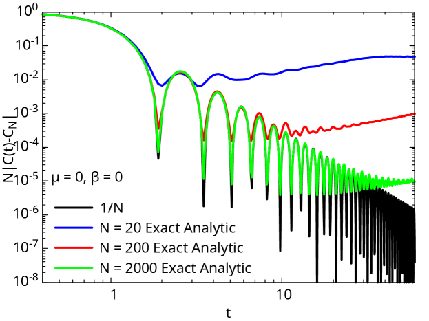
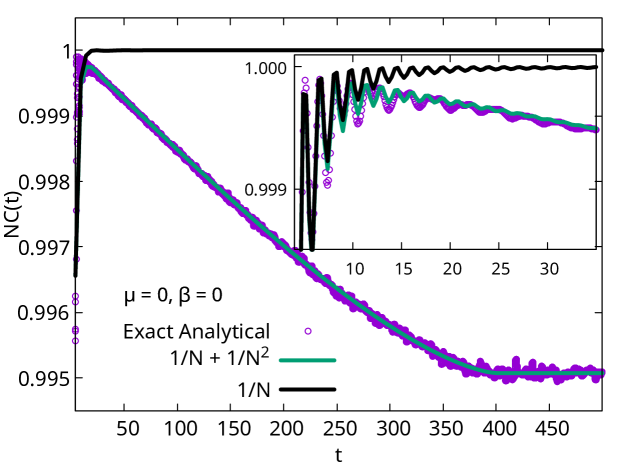
Figure 1: Time evolution of the quantum uncertainty $C(t)$ with $t$ in units of $J=1$ for $\mu=\beta=0$. Top: The blue ($N=20$), red ($N=200$), and green ($N=2000$) curves correspond to $C(t)$ given in Eq. (5) and (6) and $C_{N}=(N+1)/[(N-1)(N+2)]$. They converge to the $1/N$ prediction Eq. (8), with $C_{N}=1/N$, only for sufficiently large $N$. In both cases, $C_{N}$ is given by the time independent part of $C(t)$. Bottom: Comparison between the analytical exact $C(t)$ Eqs. (Anatomy of information scrambling and decoherence in the integrable Sachdev-Ye-Kitaev model), (5), (6) in terms of the eigenvalues of $J_{ij}$ (purple circles) with the simple analytic $C(t)$ including up to $1/N^{2}$ corrections for $N=200$ on a linear scale. The black curve stands for the $1/N$ result, Eq. (8), while the green curve stands for the $1/N+1/N^{2}$ result, Eqs. (Anatomy of information scrambling and decoherence in the integrable Sachdev-Ye-Kitaev model) and (11). The agreement between of analytical exact and the $1/N+1/N^{2}$ results is excellent for all timescales. Deviations from the $1/N$ expression occur at $t\sim\sqrt{N}$. The Heisenberg time, signaling saturation, is at $t\sim 2N$.

We now proceed with the analytical evaluation of $1/N^{2}$ terms in $C(t)$ from Eqs. (5), (6). This requires the inclusion of the two-point correlations of the eigenvalues of the coupling matrix $J_{ij}=-J_{ji}$, including self-correlations which can be expressed in terms of the spectral form factor. A simple calculation shows that,

$$C(t) = \frac{N^{2}}{\mathcal{N}}\left[1-\frac{J_{1}^{2}(2t)}{t^{2}}-K_{c}(t)\right.$$

$$\left.+\frac{1}{N}\left(1-\frac{2J_{1}(2t)\theta(2N-t)+J_{1}(4t)}{2t}\right)\right]{\mathrm{e}}^{-2\mu t},$$

where we have reinstated $\cal N$ in order to account for additional $1/N^{2}$ effects, $\theta$ is the Heaviside step function, and $N^{2}K_{c}(t)=\langle|\sum_{k=1}^{N}\exp(it\lambda_{k})|^{2}\rangle-|\langle\sum_{k=1}^{N}\exp(it\lambda_{k})\rangle|^{2}$ is the connected spectral form factor (SFF).

In the large-$N$ limit one can obtain [64, 65] an explicit analytic expression for $K_{c}(t)$ as follows. Since $J_{ij}$ is an antisymmetric random matrix (class D) whose joint eigenvalue distribution  [63, 58] coincides with that of the chiral Gaussian Unitary ensemble with topological number $\nu=-1/2$, its spectral density is a semicircle with bulk two-point correlations given by the Gaussian Unitary Ensemble. For a non-uniform spectral density, the spectral form factor is in general given by

$$K_{c}(t)=\int dx\rho(x)K_{\rm RMT}(t/\rho(x)),$$ (10)

where $K_{\rm RMT}$ is the universal RMT SFF for the appropriate ensemble. This integral is evaluated as,

$$K_{c}(t)=\begin{cases}\frac{2}{\pi N}\left(\frac{t}{2N}\sqrt{1-\frac{t^{2}}{4N^{2}}}+\arcsin(\frac{t}{2N})\right),\ t<2N\\ \frac{1}{N},\ t\geq 2N\end{cases}\!\!\!.$$ (11)

For times $t\gtrsim\sqrt{N}$, $K_{c}(t)\sim 2t/\pi N$ and then gradually saturates to $1/N$ as the Heisenberg time $t\sim 2N$ is approached. We stress that since the spectral density is not constant, the time dependence of Eq. (11) has clear deviations from linear behavior before the Heisenberg time, which translates into similar deviations in $C(t)$. Interestingly, in the range of times of interest, $2N>t>\sqrt{N}$, a simple inspection of Eq. (Anatomy of information scrambling and decoherence in the integrable Sachdev-Ye-Kitaev model) reveals that $C(t)$ is controlled by $K_{c}(t)$ despite it being of the order $1/N^{2}$ and therefore subleading in the $1/N$ expansion. The reason for that is that the time dependence of the leading $1/N$ terms approaches zero in a power-law fashion so that for $t>\sqrt{N}$ they become smaller than $K_{c}(t)$ which increases linearly in time. Crucially, the sign of the SFF term is negative, which leads to a local maximum in the OTOC not related to the small oscillations. Therefore, the OTOC decreases with time for $t>\sqrt{N}$, which corresponds to a decrease of quantum scrambling due to the discreteness of the spectrum captured by the SFF.

The results depicted in the top panel of Fig. 1 fully confirm this picture. The analytical expression for $C(t)$ Eq. (Anatomy of information scrambling and decoherence in the integrable Sachdev-Ye-Kitaev model), which includes $1/N$ and $1/N^{2}$ corrections, agrees at all times scales with the exact $C(t)$ Eqs. (Anatomy of information scrambling and decoherence in the integrable Sachdev-Ye-Kitaev model), (5), (6), at $\beta=0$, in terms of the eigenvalues of $J_{ij}$, which must be computed numerically. Substantial deviations are observed for long times if only the leading $1/N$ correction Eq. (8) is taken into account. The effect of the bath is to suppress scrambling exponentially.

We have thus found that, for $t\gtrsim\sqrt{N}$, $C(t)$ is controlled by the SFF of the random couplings $J_{ij}$, which has the expected linear behavior observed in quantum chaotic systems for times $t>\sqrt{N}$ but not too close to the Heisenberg time. This does not mean that the $q=2$ SYK is many-body quantum chaotic. While single-particle observables may show quantum chaos, the many-body dynamics are still integrable because the Majoranas are not interacting. For instance, the level statistics is Poisson. Moreover, the timescales involved are polynomial in $N$ which is typical of integrable systems. The results of Appendix A show that finite $\beta$ effects do not change qualitatively this picture.

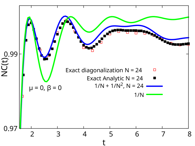
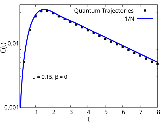
Figure 2: Top: $C(t)$ with $t$ in units of $J=1$, for $\mu=\beta=0$. $C(t)$ Eq. (Anatomy of information scrambling and decoherence in the integrable Sachdev-Ye-Kitaev model) is computed using exact diagonalization for $N=24$ (red) with $\sim 10^{6}$ disorder realizations. The exact diagonalization result shows almost no difference with respect to the exact analytic result (black) Eqs. (5), (6), and and also an excellent agreement with the $1/N+1/N^{2}$ simple expression (blue) Eq. (Anatomy of information scrambling and decoherence in the integrable Sachdev-Ye-Kitaev model). Substantial deviations are observed if only the leading $1/N$ correction (green) Eq. (8) is kept. Bottom: $C(t)$ for $\mu=0.15$, $N=18$ and $\beta=0$. We combine exact diagonalization with the quantum trajectory method [66, 67]. For each point in time, we use $200$ quantum trajectories, a time step of $dt=0.01$, and at least $5\times 10^{5}$ disorder realizations. The exponential approach to the steady state for $\mu\neq 0$ is correctly reproduced by the quantum trajectory method and we find good agreement with the $1/N$ semiclassical result.

Exact numerical results.—Previously, we carried out a comparison between simple analytical expressions depending on elementary functions, Eqs. (8) and (Anatomy of information scrambling and decoherence in the integrable Sachdev-Ye-Kitaev model), and full analytical expressions, Eqs. (5) and (6), that still require the diagonalization of a single-particle random matrix $J_{ij}$. We now compare those analytical results with a numerical calculation of $C(t)$ by exact diagonalization combined with the quantum trajectory method [68, 66, 67] when the bath is turned on ($\mu\neq 0$). The fermionic quantum trajectory method is described in Appendix B. The need of a double average over quantum trajectories and disorder realizations for $\mu>0$ limits the sizes for which we can make a detailed comparison to $N\lesssim 20$.

The results in Fig. 2 for $\mu=0$ show an excellent agreement between the compact analytical $C(t)$ Eq. (Anatomy of information scrambling and decoherence in the integrable Sachdev-Ye-Kitaev model), including $1/N+1/N^{2}$ contributions, and the exact diagonalization result. The small shift upward of the former is of order $1/N^{3}$ and therefore consistent with neglected terms in the expansion. Differences between the exact analytical $C(t)$ Eqs. (5), (6) and exact diagonalization results are barely noticeable. We stress that the comparison is parameter free and that the inclusion of $1/N^{2}$ corrections is essential for the observed level of agreement. For a finite $\mu$ (bottom plot), the numerical $C(t)$, using $200$ quantum trajectories, reproduces correctly the expected ${\rm e}^{-2\mu t}$ decay due to the bath, a feature that we derive analytically in Appendix B. Subleading features, like oscillations, are difficult to reproduce numerically because it would require a much larger number of disorder realizations. This illustrates the importance of obtaining analytic results to describe quantitatively the different stages of the quantum dynamics.
Conclusions.—We studied information scrambling and the effect of Markovian dissipation in an integrable SYK model through an analytical calculation of the growth of quantum uncertainty characterized by OTOCs at all times scales. In the absence of dissipation, the asymptotic approach to the steady state is power-law with superimposed oscillations. At $t\sim\sqrt{N}$, the overall growth of scrambling stops and starts to decrease linearly in time. This unexpected change of trend has its origin in a subleading $1/N^{2}$ correction to the OTOC that becomes dominant in this region. We show analytically that this correction is nothing but the SFF of the random couplings $J_{ij}$. It becomes dominant for $t\gtrsim\sqrt{N}$ because the SFF is linear in time, whereas the rest of the time-dependent terms in the OTOC tend to zero in a power-law fashion. For $t\approx 2N$ (the Heisenberg time), the linear decrease of the uncertainty terminates, and the uncertainty reaches saturation though we still observe small oscillatory contributions whose amplitude decreases as a power law in time. The effect of the Markovian environment is an exponential decay of the growth of quantum uncertainty at a timescale inversely proportional to the coupling to the bath, so it will eventually dominate the approach to saturation. Oscillations in time are still occur but are a subleading effect in this limit. We believe that features like a power-law decay approach to saturation together with an oscillatory behavior of the OTOC are generic features in quantum many-body integrable systems. It would be interesting to explore the dynamics of the present SYK model employing more general jump operators so that the vectorized Liouvillian has random quartic terms in order to study whether the environment can induce quantum chaotic features in the dynamics.

Acknowledgments.—AMGG thanks Klaus Mølmer for illuminating correspondence. AMGG, JPZ, and CL acknowledge support from the National Natural Science Foundation of China (NSFC): Individual Grant No. 12374138, Research Fund for International Senior Scientists No. 12350710180, and National Key R$\&$D Program of China (Project ID: 2019YFA0308603). AMGG acknowledges support from a Shanghai talent program. LS was supported by a Research Fellowship from the Royal Commission for the Exhibition of 1851. JJMV is supported in part by US DOE Grant No. DE-FAG-88FR40388.

End Matter

Appendix A Finite-temperature results

In this appendix we obtain jump operators such that the system relaxes to the thermal state [61, 56] and show that also in this case the coupling to the bath factorizes from the OTOC. We then show that finite temperature does not qualitatively change the behaviour of $C(t)$.

Finite-temperature steady state.—By an orthogonal transformation of the Majorana fermions, $\widetilde{\chi}_{i}=S_{ij}\chi_{j}$, the $q=2$ Hamiltonian of the SYK model in Eq. (1) can be rewritten as [69]

$$H=i\sum_{i<j}^{N}J_{ij}\chi_{i}\chi_{j}=i\sum_{k=1}^{N/2}\lambda_{k}\widetilde{\chi}_{2k-1}\widetilde{\chi}_{2k},$$ (12)

where $i\lambda_{k}$ are the eigenvalues of $J_{ij}$. In terms of Dirac fermions ${c}_{k}^{\dagger}=(\widetilde{\chi}_{2k-1}-i\widetilde{\chi}_{2k})/\sqrt{2}$, the Hamiltonian reads

$$H=\sum_{k=1}^{N/2}\lambda_{k}\left({c}^{\dagger}_{k}{c}_{k}-\frac{1}{2}\right)\equiv\sum_{k=1}^{N/2}H_{k}.$$ (13)

We now show that the jump operators

$$L_{k}^{(1)}=\sqrt{\mu(1-f(\lambda_{k}))}{c}_{k},\quad L_{k}^{(2)}=\sqrt{\mu f(\lambda_{k})}{c}_{k}^{\dagger},$$ (14)

where $f(\lambda)=1/(1+\exp({\beta\lambda}))$ is the Fermi-Dirac distribution, lead to the steady state density matrix $\rho=e^{-\beta H}/Z$. In terms of these jump operators, the Lindblad equation becomes

$$\mathcal{L}_{\beta}[\rho]= -i[H,\rho]+\mu\sum_{k=1}^{N/2}\Big{[}(1-f(\lambda_{k}))(2{c}_{k}\rho{c}_{k}^{\dagger}-\{{c}_{k}^{\dagger}{c}_{k},\rho\})$$

$$+f(\lambda_{k})(2{c}_{k}^{\dagger}\rho{c}_{k}-\{{c}_{k}{c}_{k}^{\dagger},\rho\})\Big{]}.$$ (15)

Since the $H_{k}$ commute among themselves and also commute with $c_{l\neq k}$ and $c_{l\neq k}^{\dagger}$, we only have to consider the commutation of the factor $\exp(-\beta H_{k})$ with $c_{k}$ and $c_{k}^{\dagger}$. Using that $c_{k}\exp(-\beta H_{k})c_{k}^{\dagger}=\exp(-\beta\lambda_{k}/2)c_{k}c_{k}^{\dagger}$, etc., one easily sees that $\mathcal{L}_{\beta}(\exp(-\beta H))=0$.

Factorization of the $\mu$-dependence.—The time evolution of $c_{p}$ and $c_{p}^{\dagger}$ is given by the adjoint Lindblad operator [56],

$$\frac{dc_{p}(t)}{dt}=\mathcal{L}^{\dagger}[{c_{p}}(t)]=+i[H,c_{p}(t)]$$

$$+\mu\sum_{k}^{N/2}\Big{[}(1-f(\lambda_{k}))(-2{c}_{k}^{\dagger}c_{p}(t){c}_{k}-\{{c}_{k}^{\dagger}{c}_{k},c_{p}(t)\})$$

$$+f(\lambda_{k})(-2{c}_{k}c_{p}(t){c}_{k}^{\dagger}-\{{c}_{k}{c}_{k}^{\dagger},c_{p}(t)\})\Big{]},$$ (16)

and the same equation for the evolution of $c_{p}^{\dagger}$. From the anti-commutation relations of the creation and annihilation operator we find

$$\frac{dc_{p}(t)}{dt}=\mathcal{L}^{\dagger}[{c_{p}}(t)]=i[H,c_{p}(t)]-\mu c_{p}(t),$$ (17)

and the same evolution equation for $c_{p}^{\dagger}(t)$. Since the Majorana operators are linear combinations of $c_{p}$ and $c_{p}^{\dagger}$ we thus find that

$$\left(\frac{d}{dt}+\mu\right)\widetilde{\chi}_{k}(t)=i[H,\widetilde{\chi}_{k}(t)].$$ (18)

Because the original Majoranas are linearly related to the $\widetilde{\chi}_{k}$ this equation also holds for the $\chi_{k}$. This shows that the $\mu$-dependence also factorizes at finite temperature.

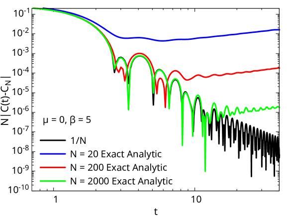
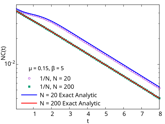
Figure 3: $C(t)$ with $t$ in units of $J=1$ for $\beta=5$. Top: $\mu=0$. The black curve stands for the semiclassical expression Eq. (A) with $C_{N}$ given by the time independent part of the coefficient of $\exp[-\mu t]$ in Eq. (A). The blue ($N=20$), red ($N=200$), and green ($N=2000$) curves stand for the exact analytic $C(t)$, Eqs. (5) and (6) with $C_{N}=0.06,0.044,0.043$ for $N=20,200,2000$, respectively. The initial approach to the steady state is still power-law, so thermal effects do not lead to qualitative changes. Bottom: $\mu=0.15,\beta=5$. For $t\gtrsim 1/2\mu$ the decay is exponential and fully controlled by the Markovian bath.

Dynamics of $C(t)$.—At finite $\beta$, the leading $1/N$ expression for $C(t)$ is [recall that at $\beta=0$ we have Eq. (7)]:

$$C(t)=\frac{1}{2N}\Bigg{[}2\int_{-2}^{2}\frac{d\lambda\rho(\lambda)}{\cosh\frac{\beta\lambda}{2}}+2\left(\int_{-2}^{2}\frac{d\lambda\rho(\lambda)\cos(\lambda t)}{\cosh\frac{\beta\lambda}{2}}\right)^{2}$$

$$-N\left(\int_{-2}^{2}\frac{d\lambda\rho(\lambda)}{\cosh\frac{\beta\lambda}{2}}\right)^{2}+N\left(\int_{-2}^{2}\frac{d\lambda\rho(\lambda)\cosh\frac{\beta\lambda}{4}}{\cosh\frac{\beta\lambda}{2}}\right)^{2}$$

$$-3\left(\int_{-2}^{2}d\lambda\rho(\lambda)\frac{\cos(\lambda t)\cosh\frac{\beta\lambda}{4}}{\cosh\frac{\beta\lambda}{2}}\right)^{2}$$

$$+\left(\int_{-2}^{2}d\lambda\rho(\lambda)\frac{\sin(\lambda t)\sinh\frac{\beta\lambda}{4}}{\cosh\frac{\beta\lambda}{2}}\right)^{2}\Bigg{]}{\rm e}^{-2\mu t}.$$ (19)

The one-dimensional integrals in Eq. (A) cannot be evaluated exactly but an asymptotic expression valid in the limit $t\gg\beta$ with $\beta$ and $\mu$ fixed is available. The most salient finite-$\beta$ effect in $C(t)$ is to induce, for intermediate times, an exponential decay $\sim e^{-\beta\pi t}$. For longer times, the approach to the steady state is power-law $\sim 1/t^{3}$ as in the $\beta=0$ case. At finite $\mu$, the asymptotic decay is exponential and $\beta$-independent, with oscillations still superimposed. Therefore, thermal effects are mostly quantitative not qualitative. This is confirmed by an explicit comparison, depicted in Fig. 3, between the $1/N$ prediction Eq. (A) and the exact $C(t)$ Eqs. (5) and (6) for $\beta=5$.

Regarding $1/N^{2}$ corrections, an analogous expression to Eq. (Anatomy of information scrambling and decoherence in the integrable Sachdev-Ye-Kitaev model) could also be worked out at finite $\beta$, although it would be rather cumbersome. Moreover, the results of Fig. 3 show that thermal effects do not induce quantitative changes in $C(t)$.

Appendix B Fermionic Quantum Trajectory Method

In this appendix, we first review the method of quantum trajectories [68, 66, 67], originally proposed in the context of bosonic systems and extend it to the fermionic systems discussed in this paper. We consider an open quantum system where the system degrees of freedom consist of $N$ bosonic fields $a_{i},i=1,\ldots,N$ with $[a_{i},a_{j}^{\dagger}]=\delta_{ij}$. When coupled to a Markovian bath, the reduced density matrix $\rho$ for the system evolves under the following master equation

$$\frac{d\rho}{dt}=-{\rm i}[H,\rho]-\mu N\rho+\mu\sum_{n}L_{n}\rho L^{\dagger}_{n}\,,$$ (20)

where $L_{n}$ are jump operators built out of the field operators $a_{i}$ and $a_{i}^{\dagger}$. Using the quantum regression theorem, the evolution equation for the Green’s functions $G_{ij}(t)=\langle a_{i}(t)a_{j}\rangle$ is given by the action of the adjoint Lindblad operator,

$$\frac{dG_{ij}}{dt}={\rm i}\langle[H,a_{i}](t)\,a_{j}\rangle-\mu NG_{ij}(t) +\mu\sum_{n}\langle(L^{\dagger}_{n}a_{i}L_{n})(t)\,a_{j}\rangle.$$ (21)

The method of quantum trajectories states that this equation is solved by

$$G_{ij}(t)=\lim_{M\to\infty}\frac{1}{M}\sum_{q=1}^{M}\langle U^{\dagger}_{q}(t)a_{i}U_{q}(t)a_{j}\rangle,$$ (22)

where each $U_{q}(t)$ is a unitary operator constructed in the following way: we first subdivide the time interval $[0,t]$ into equal segments of length $\delta t$. At each time step $k\delta t$, we generate a real number $\xi$ from the uniform distribution in $[0,1]$. Assuming the jump operators are unitary, the evolution operator from $k\delta t$ to $(k+1)\delta t$ is

$$U_{q}(k\delta t)=\begin{cases}e^{-{\rm i}H\delta t},&\textrm{if $\xi>1-e^{-\mu N\delta t/2}$}\\ L_{n},&\textrm{if $\xi<1-e^{-\mu N\delta t/2}$}\end{cases}.$$ (23)

Here, $n$ is an integer randomly sampled from the set $\{1,\ldots,N\}$ at each time step. The evolution operator $U_{q}(t)$ is then a product of these evolution operators.

$$U_{q}(t)=U(t-\delta t)U(t-2\delta t)\cdots U(\delta t)U(0).$$ (24)

In order to extend these results to fermonic systems such as the ones considered in the main text, a central issue is the anti-commutation relations of the fermionic field operators that replace the commutation relations assumed in the analysis above. When the jump operators and the fermion operators anti-commute, the quantum master equation (20) governing the evolution of the reduced density matrix can no longer be directly applied to the $n$-point function. Instead, as is shown in Appendix B of Ref. [60], the adjoint Lindblad operator acts on the Green’s function with an extra minus sign. More specifically, using the notations of the main text where $\chi_{i},i=1,\ldots,N$ are $N$ Majorana fermions with anti-commutation relations $\{\chi_{i},\chi_{j}\}=\delta_{ij}$, Eq. (21) should be replaced with

$$\frac{dG_{ij}}{dt}={\rm i}\langle[H,\chi_{i}](t)\,\chi_{j}\rangle-\mu NG_{ij}(t) -\mu\sum_{n}\langle(L^{\dagger}_{n}\chi_{i}L_{n})(t)\,\chi_{j}\rangle.$$ (25)

Note the minus sign in front of the last term. Since the rest of the equation is the same as the bosonic case considered above, we can account for this minus sign by replacing $L_{n}$ with $\widetilde{L}_{n}=\gamma_{c}L_{n}$, where $\gamma_{c}$ is the chiral fermion operator. Using the fact that $\gamma^{2}_{c}=1$ and that $\gamma_{c}$ anti-commutes with all Majorana operators, we find

$$\widetilde{L}^{\dagger}_{n}\chi_{i}\widetilde{L}_{n}=L^{\dagger}_{n}\gamma_{c}\chi_{i}\gamma_{c}L_{n}=-L^{\dagger}_{n}\chi_{i}L_{n}.$$ (26)

Therefore, replacing $L_{n}$ with $\widetilde{L}_{n}$ converts the fermionic master equation to the bosonic one. Instead of Eq. (23), we use the following quantum trajectory evolution operator to obtain the solution of Eq. (25) ,

$$\widetilde{U}_{q}(k\delta t)=\begin{cases}e^{-{\rm i}H\delta t},&\textrm{if $\xi>1-e^{-\mu N\delta t/2}$}\\ \gamma_{c}L_{n}\equiv\sqrt{2}\gamma_{c}\chi_{n},&\textrm{if $\xi<1-e^{-\mu N\delta t/2}$}\end{cases}.$$ (27)

The $\mu$-dependence of this time evolution can be worked out analytically when we consider a single time step. Since at every time step we have a probability $\mu N\delta t/2$ for a jump operator and a probability $(1-\mu N\delta t/2)$ for a Hamiltonian evolution, we have

$$\frac{1}{M}\sum_{q=1}^{M}\widetilde{U}^{\dagger}_{q}(\delta t)\chi_{i}\widetilde{U}_{q}(\delta t)=\left(1-\frac{\mu N\delta t}{2}\right) e^{iH\delta t}\chi_{i} e^{-iH\delta t}$$ (28)

$$+ \frac{\mu N\delta t}{2}\frac{(N-2)}{N}\chi_{i}=e^{iH\delta t}\chi_{i} e^{-iH\delta t}-\mu\delta t\chi_{i},$$

where we have used $\widetilde{L}_{n}\chi_{i}\widetilde{L}_{n}=\chi_{i}$ for $i\neq n$ and $\widetilde{L}_{i}\chi_{i}\widetilde{L}_{i}=-\chi_{i}$. For $q=2$ and to linear order in $\delta t$, this implies that $\chi_{i}$ satisfies the adjoint master equation Eq. (18), implying that for $\mu t\ll N$ the $\mu$-dependence factorizes as

$$G_{ij}(t)=e^{-\mu t}\langle e^{iHt}\chi_{i}e^{-iHt}\chi_{j}\rangle.$$ (29)

We emphasize that the additional minus sign in the master equation was essential to obtain the correct $\mu$-dependence [50]. Had we not included it, we would instead obtain a factor $e^{-\mu Nt}$, which is what one expects for a bosonic system.

The procedure for the four-point function considered in the main text follows by replacing both time evolutions by the right-hand side of Eq. (28) using independent trajectories. From the argument above, it is clear that the $\mu$-dependence factorizes for the four-point function as well.

References

- Larkin and Ovchinnikov [1969] A. I. Larkin and Y. N. Ovchinnikov, Quasiclassical method in the theory of superconductivity, Sov. Phys. JETP 28, 1200 (1969).
- Berman and Zaslavsky [1978] G. Berman and G. Zaslavsky, Condition of stochasticity in quantum nonlinear systems, Physica A 91, 450 (1978).
- Jalabert et al. [2018] R. A. Jalabert, I. Garc\́mathrm{i}a-Mata, and D. A. Wisniacki, Semiclassical theory of out-of-time-order correlators for low-dimensional classically chaotic systems, Phys. Rev. E 98, 062218 (2018).
- Xu et al. [2020] T. Xu, T. Scaffidi, and X. Cao, Does Scrambling Equal Chaos?, Phys. Rev. Lett. 124, 140602 (2020).
- Hummel et al. [2019] Q. Hummel, B. Geiger, J. D. Urbina, and K. Richter, Reversible Quantum Information Spreading in Many-Body Systems near Criticality, Phys. Rev. Lett. 123, 160401 (2019).
- Hashimoto et al. [2020] K. Hashimoto, K.-B. Huh, K.-Y. Kim, and R. Watanabe, Exponential growth of out-of-time-order correlator without chaos: inverted harmonic oscillator, J. High Energy Phys. 2020 (11).
- Pilatowsky-Cameo et al. [2020] S. Pilatowsky-Cameo, J. Chávez-Carlos, M. A. Bastarrachea-Magnani, P. Stránský, S. Lerma-Hernández, L. F. Santos, and J. G. Hirsch, Positive quantum lyapunov exponents in experimental systems with a regular classical limit, Phys. Rev. E 101, 010202 (2020).
- Chávez-Carlos et al. [2019] J. Chávez-Carlos, B. López-del Carpio, M. A. Bastarrachea-Magnani, P. Stránský, S. Lerma-Hernández, L. F. Santos, and J. G. Hirsch, Quantum and Classical Lyapunov Exponents in Atom-Field Interaction Systems, Phys. Rev. Lett. 122, 024101 (2019).
- Kitaev [2015] A. Kitaev, A simple model of quantum holography (2015), string seminar at KITP and Entanglement 2015 program, 12 February, 7 April and 27 May 2015, http://online.kitp.ucsb.edu/online/entangled15/.
- Bohigas and Flores [1971] O. Bohigas and J. Flores, Two-body random hamiltonian and level density, Phys. Lett. B 34, 261 (1971).
- French and Wong [1970] J. B. French and S. S. M. Wong, Validity of random matrix theories for many-particle systems, Phys. Lett. B 33, 449 (1970).
- French and Wong [1971] J. French and S. Wong, Some random-matrix level and spacing distributions for fixed-particle-rank interactions, Phys. Lett. B 35, 5 (1971).
- Sachdev and Ye [1993] S. Sachdev and J. Ye, Gapless spin-fluid ground state in a random quantum Heisenberg magnet, Phys. Rev. Lett. 70, 3339 (1993).
- Benet et al. [2001] L. Benet, T. Rupp, and H. A. Weidenmüller, Nonuniversal behavior of the -body embedded gaussian unitary ensemble of random matrices, Phys. Rev. Lett. 87, 010601 (2001).
- Maldacena and Stanford [2016] J. Maldacena and D. Stanford, Remarks on the Sachdev-Ye-Kitaev model, Phys. Rev. D 94, 106002 (2016).
- Garc\́mathrm{i}a-Garc\́mathrm{i}a and Verbaarschot [2016] A. M. Garc\́mathrm{i}a-Garc\́mathrm{i}a and J. J. M. Verbaarschot, Spectral and thermodynamic properties of the Sachdev-Ye-Kitaev model, Phys. Rev. D 94, 126010 (2016).
- Maldacena et al. [2016a] J. Maldacena, S. H. Shenker, and D. Stanford, A bound on chaos, J. High Energy Phys. 2016 (106).
- Bagrets et al. [2017] D. Bagrets, A. Altland, and A. Kamenev, Power-law out of time order correlation functions in the SYK model, Nucl. Phys. B 921, 727 (2017).
- Kitaev and Suh [2018] A. Kitaev and S. J. Suh, The soft mode in the Sachdev-Ye-Kitaev model and its gravity dual, J. High Energy Phys. 2018 (5).
- Sünderhauf et al. [2019] C. Sünderhauf, L. Piroli, X.-L. Qi, N. Schuch, and J. I. Cirac, Quantum chaos in the Brownian SYK model with large finite : OTOCs and tripartite information, J. High Energy Phys. 2019 (038).
- Gu et al. [2022] Y. Gu, A. Kitaev, and P. Zhang, A two-way approach to out-of-time-order correlators, J. High Energy Phys. 2022 (133).
- Zhang [2023] P. Zhang, Information scrambling and entanglement dynamics of complex Brownian Sachdev-Ye-Kitaev models, J. High Energy Phys. 2023 (105).
- Kobrin et al. [2021] B. Kobrin, Z. Yang, G. D. Kahanamoku-Meyer, C. T. Olund, J. E. Moore, D. Stanford, and N. Y. Yao, Many-body chaos in the Sachdev-Ye-Kitaev Model, Phys. Rev. Lett. 126, 030602 (2021).
- Garc\́mathrm{i}a-Garc\́mathrm{i}a et al. [2024a] A. M. Garc\́mathrm{i}a-Garc\́mathrm{i}a, C. Liu, and J. J. M. Verbaarschot, Sparsity-Independent Lyapunov Exponent in the Sachdev-Ye-Kitaev Model, Phys. Rev. Lett. 133, 091602 (2024a).
- Garcia-Mata et al. [2023] I. Garcia-Mata, R. Jalabert, and D. Wisniacki, Out-of-time-order correlations and quantum chaos, Scholarpedia 18, 55237 (2023).
- Cipolloni et al. [2024] G. Cipolloni, L. Erdős, and J. Henheik, Out-of-time-ordered correlators for Wigner matrices, arXiv:2402.17609 (2024).
- Torres-Herrera et al. [2018] E. J. Torres-Herrera, A. M. Garc\́mathrm{i}a-Garc\́mathrm{i}a, and L. F. Santos, Generic dynamical features of quenched interacting quantum systems: Survival probability, density imbalance, and out-of-time-ordered correlator, Phys. Rev. B 97, 060303 (2018).
- Cotler et al. [2017a] J. Cotler, N. Hunter-Jones, J. Liu, and B. Yoshida, Chaos, complexity, and random matrices, J. High Energy Phys. 2017 (48).
- Rammensee et al. [2018] J. Rammensee, J. D. Urbina, and K. Richter, Many-Body Quantum Interference and the Saturation of Out-of-Time-Order Correlators, Phys. Rev. Lett. 121, 124101 (2018).
- Nahum et al. [2018] A. Nahum, S. Vijay, and J. Haah, Operator Spreading in Random Unitary Circuits, Phys. Rev. X 8, 021014 (2018).
- von Keyserlingk et al. [2018] C. W. von Keyserlingk, T. Rakovszky, F. Pollmann, and S. L. Sondhi, Operator Hydrodynamics, OTOCs, and Entanglement Growth in Systems without Conservation Laws, Phys. Rev. X 8, 021013 (2018).
- Yoshimura and Sá [2024] T. Yoshimura and L. Sá, Theory of Irreversibility in Many-Body Quantum Systems (2024), in preparation.
- Jackiw [1985] R. Jackiw, Lower dimensional gravity, Nucl. Phys. B 252, 343 (1985).
- Teitelboim [1983] C. Teitelboim, Gravitation and Hamiltonian structure in two spacetime dimensions, Phys. Lett. B 126, 41 (1983).
- Shenker and Stanford [2015] S. H. Shenker and D. Stanford, Stringy effects in scrambling, arXiv:1412.6087 (2015).
- Maldacena et al. [2016b] J. Maldacena, D. Stanford, and Z. Yang, Conformal symmetry and its breaking in two-dimensional nearly anti-de Sitter space, Prog. Theor. Exp. Phys. 2016, 12C104 (2016b).
- Stanford et al. [2022] D. Stanford, Z. Yang, and S. Yao, Subleading Weingartens, J. High Energy Phys. 2022 (200).
- Bergamasco et al. [2023] P. D. Bergamasco, G. G. Carlo, and A. M. F. Rivas, Quantum Lyapunov exponent in dissipative systems, Phys. Rev. E 108, 024208 (2023).
- Yoshida and Yao [2019] B. Yoshida and N. Y. Yao, Disentangling Scrambling and Decoherence via Quantum Teleportation, Phys. Rev. X 9, 011006 (2019).
- Tuziemski [2019] J. Tuziemski, Out-of-time-ordered correlation functions in open systems: A Feynman-Vernon influence functional approach, Phys. Rev. A 100, 062106 (2019).
- Weinstein et al. [2023] Z. Weinstein, S. P. Kelly, J. Marino, and E. Altman, Scrambling Transition in a Radiative Random Unitary Circuit, Phys. Rev. Lett. 131, 220404 (2023).
- Zanardi and Anand [2021] P. Zanardi and N. Anand, Information scrambling and chaos in open quantum systems, Phys. Rev. A 103, 062214 (2021).
- Huang et al. [2020] K.-Q. Huang, J. Wang, W.-L. Zhao, and J. Liu, Chaotic dynamics of a non-Hermitian kicked particle, J. Phys. Condens. Matter 33, 055402 (2020).
- Syzranov et al. [2018] S. V. Syzranov, A. V. Gorshkov, and V. Galitski, Out-of-time-order correlators in finite open systems, Phys. Rev. B 97, 161114 (2018).
- Zhai and Yin [2020] L.-J. Zhai and S. Yin, Out-of-time-ordered correlator in non-Hermitian quantum systems, Phys. Rev. B 102, 054303 (2020).
- Yoshimura and Sá [2024] T. Yoshimura and L. Sá, Robustness of quantum chaos and anomalous relaxation in open quantum circuits, Nat. Commun. 15, 9808 (2024).
- Garc\́mathrm{i}a-Garc\́mathrm{i}a et al. [2024b] A. M. Garc\́mathrm{i}a-Garc\́mathrm{i}a, J. J. M. Verbaarschot, and J.-P. Zheng, Lyapunov exponent as a signature of dissipative many-body quantum chaos, Phys. Rev. D 110, 086010 (2024b).
- Sá et al. [2022] L. Sá, P. Ribeiro, and T. Prosen, Lindbladian dissipation of strongly-correlated quantum matter, Phys. Rev. Research 4, L022068 (2022).
- Kulkarni et al. [2022] A. Kulkarni, T. Numasawa, and S. Ryu, Lindbladian dynamics of the Sachdev-Ye-Kitaev model, Phys. Rev. B 106, 075138 (2022).
- Garc\́mathrm{i}a-Garc\́mathrm{i}a et al. [2023] A. M. Garc\́mathrm{i}a-Garc\́mathrm{i}a, L. Sá, J. J. M. Verbaarschot, and J. P. Zheng, Keldysh wormholes and anomalous relaxation in the dissipative Sachdev-Ye-Kitaev model, Phys. Rev. D 107, 106006 (2023).
- Fortes et al. [2019] E. M. Fortes, I. Garc\́mathrm{i}a-Mata, R. A. Jalabert, and D. A. Wisniacki, Gauging classical and quantum integrability through out-of-time-ordered correlators, Phys. Rev. E 100, 042201 (2019).
- Mori [2024] T. Mori, Liouvillian-gap analysis of open quantum many-body systems in the weak dissipation limit, Phys. Rev. B 109, 064311 (2024).
- Belavin et al. [1969] A. A. Belavin, B. Y. Zeldovich, A. M. Perelomov, and V. S. Popov, Relaxation of quantum systems with equidistant spectra, Sov. Phys. JETP 29, 145 (1969).
- Lindblad [1976] G. Lindblad, On the generators of quantum dynamical semigroups, Commun. Math. Phys. 48, 119 (1976).
- Gorini et al. [1976] V. Gorini, A. Kossakowski, and E. C. G. Sudarshan, Completely positive dynamical semigroups of -level systems, J. Math. Phys. 17, 821 (1976).
- Breuer and Petruccione [2002] H.-P. Breuer and F. Petruccione, The theory of open quantum systems (Oxford University Press, Oxford, 2002).
- Manzano [2020] D. Manzano, A short introduction to the Lindblad master equation, AIP Advances 10, 025106 (2020).
- Gross and Rosenhaus [2017] D. J. Gross and V. Rosenhaus, A generalization of Sachdev-Ye-Kitaev, J. High Energy Phys. 2017 (93).
- Blocher and Mølmer [2019] P. D. Blocher and K. Mølmer, Quantum regression theorem for out-of-time-ordered correlation functions, Phys. Rev. A 99, 033816 (2019).
- Schwarz et al. [2016] F. Schwarz, M. Goldstein, A. Dorda, E. Arrigoni, A. Weichselbaum, and J. von Delft, Lindblad-driven discretized leads for nonequilibrium steady-state transport in quantum impurity models: Recovering the continuum limit, Phys. Rev. B 94, 155142 (2016).
- Prosen [2008] T. Prosen, Third quantization: a general method to solve master equations for quadratic open Fermi systems, New J. Phys. 10, 043026 (2008).
- Ullah and Porter [1963] N. Ullah and C. Porter, Invariance hypothesis and Hamiltonian matrix elements correlations, Phys. Lett. 6, 301 (1963).
- Mehta [2004] M. L. Mehta, Random matrices (Academic Press, 2004).
- Brézin and Hikami [1997] E. Brézin and S. Hikami, Spectral form factor in a random matrix theory, Phys. Rev. E 55, 4067 (1997).
- Forrester [2021] P. J. Forrester, Quantifying Dip–Ramp–Plateau for the Laguerre Unitary Ensemble Structure Function, Commun. Math. Phys. 387, 215–235 (2021).
- Mølmer et al. [1993] K. Mølmer, Y. Castin, and J. Dalibard, Monte Carlo wave-function method in quantum optics, J. Opt. Soc. Am. B 10, 524 (1993).
- Dum et al. [1992] R. Dum, P. Zoller, and H. Ritsch, Monte Carlo simulation of the atomic master equation for spontaneous emission, Phys. Rev. A 45, 4879 (1992).
- Dalibard et al. [1992] J. Dalibard, Y. Castin, and K. Mølmer, Wave-function approach to dissipative processes in quantum optics, Phys. Rev. Lett. 68, 580 (1992).
- Cotler et al. [2017b] J. S. Cotler, G. Gur-Ari, M. Hanada, J. Polchinski, P. Saad, S. H. Shenker, D. Stanford, A. Streicher, and M. Tezuka, Black holes and random matrices, J. High Energy Phys. 2017 (118).