Can solvents tie knots? Helical folds of biopolymers in liquid environments.

Abstract

Helices are the quintessential geometric motif of microscale self–assembly, from $\alpha$–helices in proteins to double helices in DNA. Assembly of the helical geometry of biopolymers is a foundational step in a hierarchy of structure that eventually leads to biological activity.

Simulating self–assembly in a simplified and controlled setting allows us to probe the relevance of the solvent as a component of the system of collaborative processes governing biomaterials. Using a simulation technique based on the morphometric approach to solvation, we performed computer experiments which fold a short open flexible tube, modelling a biopolymer in an aqueous environment, according to the interaction of the tube with the solvent alone. Different fluid environments may favour quite different solute geometry: We find an array of helical geometries that self–assemble depending on the solvent conditions, including overhand knot shapes and symmetric double helices where the strand folds back on itself. Interestingly these shapes—in all their variety—are energetically favoured over the $\alpha$–helix. In differentiating the role of solvation in self–assembly our study helps illuminate the energetic background scenery in which all soluble biomolecules live, indeed our results demonstrate that the solvent is capable of quite fundamental rearrangements even up to tying a simple overhand knot.

1 Introduction

Solvation is the physics of molecules in fluids, the collection of spontaneous processes resulting in the energetically favourable (re)arrangement of the molecule within the fluid. Solvation is one of the key mechanisms through which the aqueous environment of soluble biomolecules, such as proteins and nucleic acids, affects their structure, stability and functioning [52, 2, 39]. At a fundamental level, the solvent mediates between chemistry and structure, as a chaperon to other more concrete processes. The capacity of the solvent by itself receives little attention; the water surrounding is arguably the most challenging part of the modelling of a soluble biomolecule and therefore the development of accurate yet computationally efficient models is of central importance [37]. Details tend to be on the atomic level, specific to a particular protein, and do not address the behaviour of a general soluble polymer in a general solvent.

Biopolymer chains wind themselves into a plethora of shapes in nature. The optimal $\alpha$-helix and $\beta$-sheet forms are the fundamental motifs found in protein structures. DNA, itself a double helix, can exhibit a variety of geometric forms, which helps to expose certain base pairs along the strand [17]. Knotted configurations are found in biopolymers in wide variety of settings, where their geometric form is related to their functionality [30, 45]. The broader zoo of optimal shapes of short flexible biopolymers (see Fig. 1), and their contribution to biological function, is a rich field of research. From this broader perspective, we investigate how a fluid environment may affect the shape of a short tube–like string. Understanding form through experimentation with simple geometric objects under physically motivated constraints provides interesting insights; our optimal forms contain helical motifs known for their optimal packing upon confinement [32], and our results establish the thermodynamic stability of the overhand knot and double helix in solution.

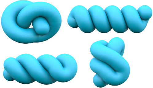
Figure 1: An array of helical forms of a flexible tube, which are relevant to biopolymer foldings. Clockwise from top left, an overhand knot, the optimal helix, a compact structure with curve motifs arranged in parallel, and a double helix folded back on itself.

Modelling the effect of the solvent on the structure of large (polyatomic) biomolecules like globular proteins is challenging: A protein’s configuration is governed by a fine balance between intramolecular bonding energy and the free energy of solvation of the fluid system [6, 44]. Whilst including the solvent explicitly in state models may enable a more complete picture of the solvent–solute interaction, the additional computational cost means there is little possibility to explore complex solute geometries let alone solvent induced shape change [52]. These difficulties motivate the development of implicit solvent models, which treat the solvent as a continuous medium, with application in molecular dynamics simulations to efficiently simulate biomolecules like proteins and nucleic acids in solution [36, 43]. Implicit solvent models make use of the geometric properties of the space occupied by the solute within the liquid in order to compute the free energy of the liquid [8].

Of interest therefore is the space-filling representation of a molecule or solute expanded by the solvent’s radius, known as the solvent-accessible surface [24]. Early solvation free energy models were often based on the volume excluded by this surface which has an entropic cost to the energy [46, 27], as well as the surface area [38, 9].

This link between geometry and the thermodynamics of fluids was made more precise through the development of the morphometric approach to modelling solvation [33, 42, 23]. In this approach the solvation free energy, $\mathbf{F}_{\mathrm{sol}}$ in (1), is given as a linear sum of the basic rigid motion invariant valuations, the volume $\mathrm{V}$, surface area $\mathrm{A}$ and two further measures of curvature $\mathrm{C}$ and $\mathrm{X}$ of the body bounded by the solvent accessible surface ($\mathcal{B}$). The thermodynamic coefficients coupling to the geometric measures are $\mathrm{p}>0$ the fluid pressure, $\sigma<0$ the planar surface tension and $\kappa$, $\bar{\kappa}\in\mathbb{R}$ for which there is no physical interpretation [23, 42, 13].

$$\mathbf{F}_{\mathrm{sol}}=\mathrm{p}\mathrm{V}(\mathcal{B})+\sigma\mathrm{A}(\mathcal{B})+\kappa\mathrm{C}(\mathcal{B})+\bar{\kappa}\mathrm{X}(\mathcal{B})\,.$$ (1)

These four geometric functions, the measures of curvature, appear as a novel application of Hadwiger’s characterisation theorem of integral geometry [13]. The measures $\mathrm{C}$ and $\mathrm{X}$ are computed as the mean and Gaussian curvatures integrated over the boundary of $\mathcal{B}$ provided this is sufficiently regular as to allow an interpretation of curvature functions [28]. By the Gauss–Bonnet theorem $\mathrm{X}=4\pi\chi$ where $\chi$ is the Euler characteristic.

The real advantage of this approach is that it (de)couples physics and geometry in a computationally convenient manner. The thermodynamic coefficients $\mathrm{p}$, $\sigma$, $\kappa$ and $\bar{\kappa}$ depend only the physical properties of the fluid, like temperature and the chemical coupling between the solvent and solute, not on the shape of the solute. These can be determined by fitting free energy values as obtained from (1) to those computed from solvent models of the statistical–mechanical theory, as tested with simple solute geometries. Once the coefficients are given, the free energy is evaluated from the geometry of $\mathcal{B}$. If $\mathcal{B}$ is modelled as a union of balls, deep results from computational topology ensure lead to the development of fast algorithms which evaluate $\mathrm{V}(\mathcal{B})$, $\mathrm{A}(\mathcal{B})$, $\mathrm{C}(\mathcal{B})$ and $\mathrm{X}(\mathcal{B})$ exactly and efficiently, fairly independently of the shape [7, 8].

For fluid systems like that of a protein within the aqueous environment of the cell, the morphometric approach can compute free energy values of complex solute geometries in excellent agreement with the classical theory at a fraction of the computational cost, making a geometric centered investigation of solvation even feasible [42].

Previously the morphometic approach was used to demonstrate that different solvent environments favoured different helical tubular solutes [15]. This was shown by comparing the solvation free energy between a collection of tight periodic helical tubes, winding such that each successive turn sits on the previous [40]. Energetically favourable configurations included the $\alpha$–helix, slightly unwound helices, resembling topologically an open infinite cylinder, and stacked parallel curves representing the infinite $\beta$–sheet structure. Our work is a considerable extension of this study by allowing the tubular solute to freely self–assemble without a priori assuming helical like curve arrangements. When considering finite strings the preference for tight single helical structures is challenged by our findings here.

The morphometric approach has also been used in a variety of settings to analyse minimising configurations [42, 16, 10], as well as for the geometric simulation of hard sphere clusters in fluids, where helical stacks of sphere were found under particular fluid conditions [48].

In this study, we will use the morphometric approach to solvation as a basis for simulating the self–assembly of a finite flexible tube, modelling a biopolymer in aqueous environments, according to the interaction of the tube with the solvent alone. We detail the results of these simulations below.

1.1 Helical folds in solvation simulations

We simulated the self–assembly of energetically favourable configurations of (unit radius) strings of length $\ell=25$ within a range of fluid conditions. This was achieved through computer experiments which optimise the shape of an open equilateral polygonal curve of fixed length, modelling the shape of the solute, according to the morphometric description of the free energy of solvation (1). The free energy is minimised via the method of simulated annealing: the curve shape is incrementally improved using a crank-shaft move while ensuring that the flexible tube does not intersect itself (see methods for details). The self–assembly of a double helical configuration via this computation method is shown in Fig. 2. The simulation is initialised in the fully solvated state and progresses to fold. First the tube comes into self–contact, causing the solvent–accessible surface to self–intersect thereby decreasing the volume and, as the leading order term in (1), thus the energy. The shape then advances as controlled by the specific linear combination of the measures given in (1) i.e. the fluid environment.

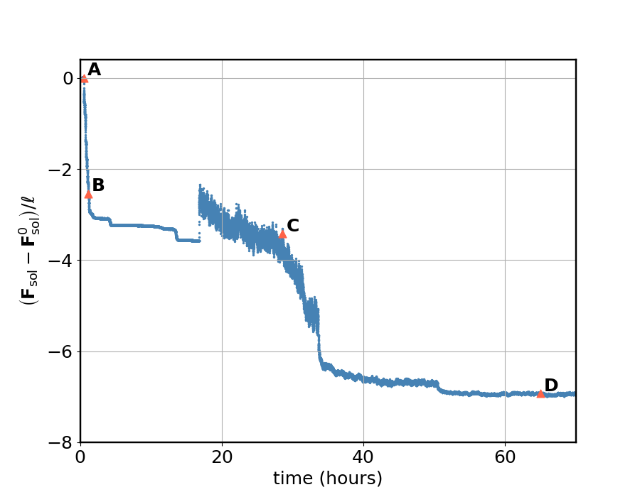
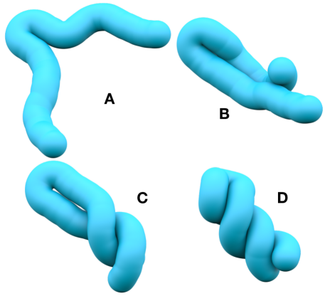
Figure 2: (Top) The solvation free energy of a tube during a simulation run, measured by $(\mathbf{F}_{\mathrm{sol}}-\mathbf{F}_{\mathrm{sol}}^{0})/\ell$, which is the free energy per unit length relative to the free energy of the fully solvated state. The tube initially comes into self–contact, as shown in configurations A and B, causing the solvent–accessible surface (not shown in the figure) to self–intersect thereby decreasing the volume and, as the leading order term in (1), thereby the energy. In configurations C and D the shape assembles as controlled by the specific linear combination of the geometric measures. Here, the packing fraction is $\eta=0.375$ and the solvent radius $r_{s}=0.2$. The lowest energy configuration is the double helical shape (D).

Modelling the solvent as a hard sphere fluid, the physical coefficients in (1) may be derived explicitly as functional expressions of the solvent packing fraction $\eta$ and solvent radius $r_{s}$, providing a way to systematically compare favorable solute geometries in different hard sphere fluid environments [14]. The range of fluid environments, $0.02\leq r_{s}<0.2$ and $\eta\in(0,0.494)$ serves as a reference model for the fluid environment of a cell under physiological conditions [42].

The landscape of optimal configurations corresponding to such fluids are shown in the phase diagram in Fig. 3. A square in the diagram corresponds to coordinates $(\eta,r_{s})$ defining a particular fluid environment, the colouring gives information of the configuration of lowest energy. The diagram was constructed using empirical classification, where structures are grouped by key distinguishing features, despite their geometries differing slightly. For example, a double helix along a straight axis is grouped together with one that is slightly bent, as their distinguishing feature is their double helical character. Additional simulations using an input of various favourable configurations under differing fluid conditions were performed to interpolate between initial simulations in the phase diagram. The final results of the phase diagram were enhanced by calculations of $\mathbf{F}_{\mathrm{sol}}$ for the collection of tight helical tubes known for their high degree of thermal stability [15].

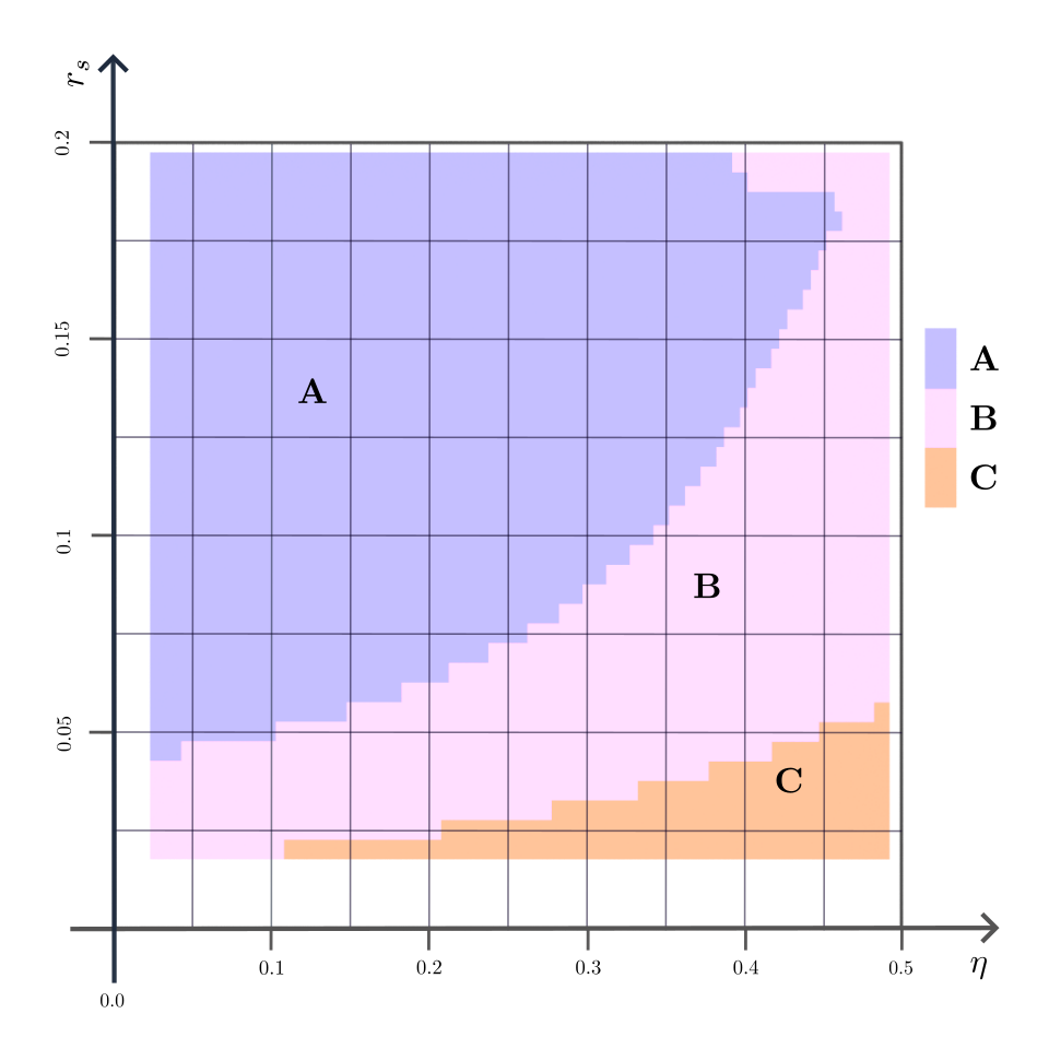
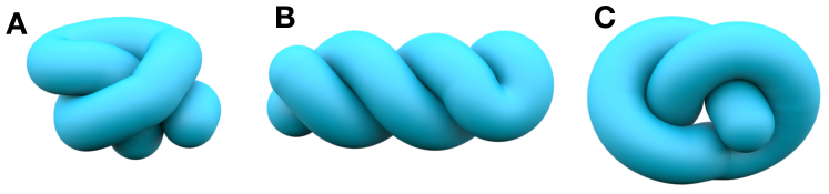
Figure 3: Phase diagram of optimal string geometries over the space of fluid properties, as defined by the solvent packing fraction $\eta$ and the relative size of the solvent given by the solvent radius $r_{s}$. The diagram splits into three regions, each with a different minimising geometry. These three geometries are shown below the diagram, and are called configurations A, B (a double helix), and C (an overhand knot).

We observe three main regions of the phase diagram, each with a given optimal form. The three configurations (shown in Fig. 3) consist of:

• Configuration A: the two ends form a basic over and under crossing, the rest of the length of the curve winds around akin to a single helix doubling back on itself. Appears at medium to large solvent radius across all packing fractions.

• Configuration B: a double helix, where the string folds back on itself. Occurs for smaller solvent radius, and it more typical for higher packing fractions.

• Configuration C: overhand knot. Appears where the solvent radius is small across all packing fractions.

The phase diagram contains previously unseen optimal curve shapes challenging the established idea that the $\alpha$-helix and $\beta$-sheet are the most energetically favourable shapes among biopolymers from the persepctive of solvation free energy [47, 15]. The appearance of the overhand knot as a stable solvation free energy minimiser could provide a basis for the existence of knotted configurations in biopolymers.

To explore the relative energies of these structures consider two cross-sections through the phase diagram, at $r_{s}=0.04$ and $r_{s}=0.125$, shown in Fig. 4.

The energies are plotted against the fluid packing fraction $\eta$ for example shapes of the groups A, B and C, including two additional configurations, the open tight helical curve of lowest energy within the collection of all tight helical curves and a low energy compact shape without otherwise recognizable structure (arising from the computer experiments). In both plots for low packing fractions all of the structures have comparable free energy values, whereas for larger packing fractions, the structures differentiate from each other significantly. This suggests that solvation forces become increasingly relevant to self–assembly as the solvent becomes denser and the size of the solute larger. This places particular importance on the configurations B and C, the double helix and the overhand knot shape, which have significantly lower energy than other structures in the region where they are most favorable. These plots also show that the energy values of tight (single) helices are well above those of the minimising configurations identified here. A full phase diagram of tight helical configurations, periodic and finite curves of the same length as the solute geometries considered here, are given in the supplementary materials. Single helices self–assemble in experiments in the region A for packing fraction $\eta\lessapprox 0.15$ with energy values close to those curves of lowest energy, in agreement with the energy data shown in Fig. 4 (b). We note that the free energy of a $\beta$-sheet configuration for a finite string is significantly higher than these values, and thus not important for our study. Finally for the fluid conditions considered in this work the fully solvated state is not a favourable configuration so that the solvent is, to a certain degree, shape determining.

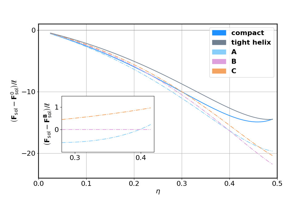
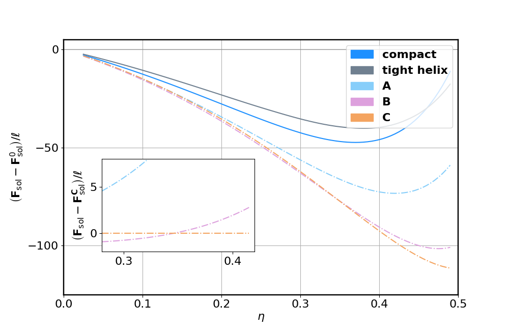
Figure 4: The free energy of solvation of a selection of low energy curve shapes plotted against the packing fraction $\eta$ for fixed solvent radius $r_{s}=0.125$ (top) and $r_{s}=0.04$ (bottom). The free energy is normalised with respected to the fully solvated state per (scale–invariant) unit length. The optimal configurations $\mathbf{A}$, $\mathbf{B}$, $\mathbf{C}$ are shown relative to the tight helix of lowest energy, and a low energy compact shape as generated from computational experiments. (top) The dominant curve shape for low $\eta$ is $\mathbf{A}$ then eventually $\mathbf{B}$ (double helix) as the packing fraction $\eta\gtrapprox 0.4$ increases. The energy differences between all structures for low $\eta$ are marginal, the energy of curve shapes $\mathbf{A}$, $\mathbf{B}$ are close for all packing fractions. Inset depicts the free energy of $\mathbf{A}$, $\mathbf{B}$ and $\mathbf{C}$ normalised with respect to the energy of shape $\mathbf{B}$. (bottom) The dominant curve shape is $\mathbf{B}$ (double helix) for low $\eta$ and $\mathbf{C}$ (overhand knot) for $\eta\gtrapprox 0.35$. Configuration $\mathbf{A}$ is the minimiser in the limit $\eta\rightarrow 0$ ($\eta\lessapprox 0.04$). For low $\eta$, the energy differences between all configurations are marginal. As the packing fraction increases $\eta\gtrapprox 0.2$ the curve shapes $\mathbf{B}$ and $\mathbf{C}$ are of significantly lower energy as compared to the other configurations. Inset depicts the free energy of $\mathbf{A}$, $\mathbf{B}$ and $\mathbf{C}$ normalised with respect to the energy of shape $\mathbf{C}$.

1.2 Discussion

In this work we utilise the morphometric approach to investigate thermodynamically favourable configurations of a tubular string solute in a hard sphere solvent, as a test case of a short biopolymer living in a fluid environment of the cell under physiological conditions. Our computer experiments demonstrate the self–assembly of the solute into a variety of helical forms using only the interaction with the solvent. We find that the overhand knot and double helix configurations are the most stable assemblies in the large region of the phase diagram where solvation plays the most significant role, proving more stable than the optimal helix seen in protein $\alpha$-helices.

We observe that solvation is more likely to be shape determining for larger solutes (small solvent radius) as the energy difference between low energy configurations is large for such fluid conditions. This implies that for such systems the solvent may play a key role in establishing shape change of biopolymers in particular by giving preference to configurations B and C. By allowing the tubular geometry to freely form, our observations are a fundamental extension of previous studies of tubular strings in fluid evironments [15] or helical tubes optimised for their compactness properties [47] demonstrating a much richer variety of thermodynamically stable structures. In the limit case $\eta\rightarrow 0$ our results display similar motifs to the entropic packing of tubular strings [32], and by including solvation effects our work may be seen as an essential progression of that study.

For small solutes and low packing fraction (Fig. 4 (b)) there is little energy difference between compact curve configurations of otherwise nonspecific geometry and tight helical geometries like the open $\alpha$–helix configuration. This implies that hard sphere fluids of large solvent radius and low packing fraction make minimal interference with respect to the solute configuration. In biomaterials like proteins, the energetic stability of the $\alpha$–helix comes from both the solvation free energy and hydrogen bonding of the backbone chain of protein molecule and interactions of the side chain atoms [19]. Our experiments show that for short strings, helical curves are simply unfavourable in comparison to other geometries; this may indicate that for short linear-chain molecules the energetic gains of hydrogen bonding is the significant factor determining the formation and prevalence of the $\alpha$-helix. It is interesting how the balance of bonding energies and the solvation free energy may compare for structures similar to the double helical configuration $\mathbf{B}$ and overhand knot $\mathbf{C}$, in particular the overhand knot was shown optimal for certain stiffness regimes of semi–flexible polymers [31, 29].

The empirical classification of the optimal curve shapes becomes increasingly coherent with decreasing solvent radius and increasing packing fraction. Within this part of the diagram two optimal shapes are distinguished, a double helix and an overhand knot. There is no apparent shape variation among the overhand knot configurations observed in region C. This shape, which is of significantly less energy than other configurations within region C has, to the best of our knowledge, not yet been recognised for its thermodynamic stability. The past years have seen extensive interest in the science of knotted proteins and biopolymers; both from the perspectives of design and function [1, 51, 50]. The observation that a short homogeneous tube will adopt a knotted structure based only on interactions with a solvent is an important step in understanding self–assembly in aqueous environments. Because of the propensity for the tube to come into self–contact, these structures also relate to ideal knots, which are length minimising configurations of knotted loops. In essence, the minimisation of length (or maximisation of radius) is a related idea that utilises geometric quantities as a measure of energy [21, 49, 11], with a deep correlation to DNA electrophoresis [49], and consequences for mechanics [18, 12].

The double helical motif, an ubiquitous shape in biology, is reminiscent here of the plectoneme geometry adopted by supercoiled DNA [3]. As with single helices these shapes are interesting from many different energetic perspectives [20]. Our attention to solvation in the simple setting of our experiments confirms the thermodynamic stability of double helical geometry, in particular over other configurations.

The major challenge of this work is the computation time needed for experiments, with this hindering a similarly in depth study of longer solute geometries.

If the solvent radius is small, the neighbourhood search about a configuration is less effective increasing the computation time of experiments. The computation time is also effected by the packing fraction (because this influences the weighting of the measures in (1)), experiments with larger $\eta$ require longer computation times. In turn this effects the reliability of the results in the corresponding regions of the phase diagram (Fig. 3) as far fewer experiments within the bottom horizontal and far right vertical stripes of the diagram were completed to conclusion from a fully solvated initial configuration. For $r_{s}<0.04$ over all packing fractions experiments were initialised in configurations similar to those shown in $\mathbf{A}$ and $\mathbf{B}$ of Fig. 2. Beyond energy specific influences on the computation time, interestingly some curve shapes seem to fold quicker than others. For example, the overhand knot shape $\mathbf{C}$ is the optimal configuration found by the algorithm in a much larger area of the phase diagram (Fig. 3) than indicated by the corresponding region. Within the testing thus far it is unclear if this is a ramification of the specific algorithm design or providing information of the energy landscape surrounding particular low energy configurations or of the folding pathways of such shapes.

An important consideration in this study is the string length.

An investigation of the effect of length on the self–assembly process is important to realise, but is made difficult by the computational limitations discussed above. Remarkably, whilst our empirical classification of energetically significant shapes is not technologically sophisticated, it was simple to implement. It seems unlikely that an empirical classification can be made so easily for longer strings; the low energy configurations in region $\mathbf{A}$ of the diagram show quite some variety in shape even for the short strings considered in this work. Without a better understanding of low energy curve motifs, the analysis of results, even if they were readily available, may require a different mechanism of sorting than geometry alone.

In summary, our geometry focused investigation provides examples of favourable biopolymer configurations, via the optimisation of unconstrained flexible tubes, inaccessible within the framework of all–inclusive molecular dynamics simulations. In differentiating the role of solvation in biopolymer reorganisation, our study helps illuminate the energetic background scenery in which all soluble biomolecules live.

2 Methods

We investigated short tubular solutes in water-like environments by way of computer simulation. The simulation tool functions as a geometric optimisation algorithm which modifies iteratively the shape of the solute body thereby decreasing the solvation free energy of the system.

Let the physical parameters, solvent radius $r_{s}$ and coefficients $\mathrm{p}$, $\sigma$, $\kappa$ and $\bar{\kappa}$, describing the thermodynamic interaction between the solute and solvent be given. The free energy of the system is computed using equation (1) with the body

$$\mathcal{B}=\bigcup_{i=1}^{n}\mathrm{B}_{r_{t}+r_{s}}(v_{i})$$

for vertices $\{v_{1},\dots,v_{n}\}$ arranged linearly on an open equilateral polygon with edge length $e$, ball radius $r_{t}>\tfrac{e}{2}$ and solvent radius $r_{s}>0$.

Here $n=101$, $e=0.25$ and $r_{t}=1.00778$ so that the scale–invariant length $\ell=\tfrac{25}{r_{t}}=24.8065$, these numbers are set for comparison with other solute geometries of finer discretisation. The vertex set $\{v_{1},\dots,v_{n}\}$ is synonymous with the open equilateral polygon and we refer to both as simply the curve.

Our algorithm evaluates approximate solutions to the following problem: What is the shape of a curve, representing a physical (re)arrangement of the body $\mathcal{B}$, which minimise the free energy of solvation?

A physical (re)arrangement of the solute body is if the $r_{t}$–balls centered on the vertices of the curve curve overlap only along the curve; such that the solute appears as a self–avoiding tube. We characterise this mathematically using the following property [35]; a curve satisfies the simple–tube property for the ball radius $r$ if for any pair $(i,j)$, $1\leq j\leq n$

$$\mathrm{B}_{r}(v_{i})\cap\mathrm{B}_{r}(v_{j})\subset\mathrm{B}_{r}(v_{k})\,\,k=i+1,\dots,j-1\,.$$ (2)

If a curve satisfies the simple tube property for a ball radius $r$ then the four geometric measures; volume $\mathrm{V}$, surface area $\mathrm{A}$ etc. included in equation (1), are constant, depending only on the geometric parameters $n$, $e$ and $r$, independent of the specific shape of the curve. This is an elementary computation following from property (2) (see supplementary materials). In particular, the volume of a solute body modelled by a curve satisfying property (2) for the radius $r_{t}$ will be constant and independent of the actual shape of the solute.

As we are interested in energetically driven shape (re)arrangement of the solute body, we say a curve models a physical (re)arrangement of the (same) solute if the curve (fixed by the parameters $n$, $e$) satisfies the simple–tube property for the radius $r_{t}$ and restrict our attention to minimising the energy on this set.

The simple–tube property distinguishes an important class of solute configurations: a configuration is called fully solvated if the curve satisfies the simple–tube property for the radius $(r_{t}+r_{s})$. Since in this case, all four geometric measures terms of equation (1) are constant and independent of the specific curve shape, the free energy of any fully solvated configuration is constant. This energy, denoted as $\mathbf{F}_{\mathrm{sol}}^{0}$, is the zero from which we measure geometry with respect to energy, and is subtracted from the computed energy values as shown in the graphs in Fig. 2 and in Fig. 4.

The simple–tube property is a discrete analog of the self–contact condition used to derive the collection of tight helical curves used as a basic test geometry in the investigation of favrouable solute geometry with respect to solvation [40, 25, 11, 4]. Importantly the property establishes that our interest is in curves satisfying the simple–tube property for the radius $r_{t}$ but not for the radius $(r_{t}+r_{s})$.

The algorithm is based on the technique of parallel simulated annealing [26]. Once the energetic and geometric parameters as described above are defined, the algorithm is initialised with a chosen curve shape. A single iteration generates a random curve close in shape to the current curve and decides whether to accept this new curve as the input of the next iteration.

Acceptance is decided by evaluating the energy difference between the current and new curves ($\Delta\mathbf{F}_{\mathrm{sol}}=\mathbf{F}_{\mathrm{sol}}^{\mathrm{new}}-\mathbf{F}_{\mathrm{sol}}^{\mathrm{cur}}$) and applying the metropolis criterium: If the new curve is of less energy it is accepted, otherwise it is accepted with probability $\mathsf{p}_{\lambda}=\exp{\left(\dfrac{-\Delta\mathbf{F}_{\mathrm{sol}}}{\lambda}\right)}$ for $\lambda\in\mathbb{R}_{>0}$.

The algorithm computes iterations of $m\approx 20$ curves in parallel with constant $\lambda$ for a time interval typically $\approx 20$ hours. During the simulation the parameter $\lambda$ generally decreases, this decreases the likelihood that configurations which increase the energy of the system are accepted. Between intervals parallel systems may be duplicated or discontinued by mixing the states between the $m$ processors according to the probability

$$\dfrac{\mathsf{p}_{\lambda}(j)}{\sum_{j=1}^{m}\mathsf{p}_{\lambda}(j)}$$

where

$$\mathsf{p}_{\lambda}(j)=\exp{\left(\dfrac{\mathbf{F}_{\mathrm{sol}}^{j}-\mathbf{F}_{\mathrm{sol}}^{0}}{\lambda}\right)}$$

and $\mathbf{F}_{\mathrm{sol}}^{j}$ is the free energy of the curve of the $j$^th processor. The energy is computed using the POWERSASA software which evaluates the measures of (1) exactly with state of the art efficiency [22].

The algorithm generates a random curve close in shape to the current curve via so–called crankshaft deformations [34]— two vertices are chosen randomly along the curve and the vertices between these two are rotated a random angle about the axis defined by the line connecting the two vertices. Here basic adaptations are included to ensure that the end vertices of the chain are translated as often as the interior vertices of the chain. This deformation preserves the number of vertices and edge lengths in a straight forward way but may produce a curve which does not model the solute body i.e. does not satisfy the simple–tube property for the radius $r_{t}$.

A second procedure checks if the curve bends too much causing kinks or different sections of the tube overlap, implying the simple–tube property for the radius $r_{t}$ is violated, in which case the curve is discarded and a new random curve is generated. This process is comparable to the computation of thickness of discrete knots and links when minimising for ropelength [41].

We are interested in comparing thermodynamically favourable solute geometries between different physiological fluid environments of biopolymers. We achieve this by using explicit formulas of the coupling coefficients $\mathrm{p}$, $\sigma$, $\kappa$ and $\bar{\kappa}$ in terms of the packing fraction of the fluid $\eta$ and the relative size of the solvent $r_{s}$ [14].

These formulaic expressions are as follows;

$$\mathrm{p} =\left(\frac{3}{4\pi}\frac{1}{r_{s}^{3}}\right)\eta\frac{1+\eta+\eta^{2}-\eta^{3}}{(1-\eta)^{3}}$$ (3)

$$\sigma =-\left(\frac{3}{4\pi}\frac{1}{r_{s}^{2}}\right)\eta\left(\frac{1+2\eta+8\eta^{2}-5\eta^{3}}{3(1-\eta)^{3}}+\frac{\ln(1-\eta)}{3\eta}\right)$$

$$\kappa =\left(\frac{3}{4\pi}\frac{1}{r_{s}}\right)\eta\left(\frac{4-10\eta+20\eta^{2}-8\eta^{3}}{3(1-\eta)^{3}}+\frac{4\ln(1-\eta)}{3\eta}\right)$$

$$\bar{\kappa} =\left(\frac{3}{4\pi}\right)\eta\left(\frac{-4+11\eta-13\eta^{2}+4\eta^{3}}{3(1-\eta)^{3}}-\frac{4\ln(1-\eta)}{3\eta}\right)\,.$$

The code can be accessed from Github [5].

Acknowledgements Funded by the Deutsche Forschungsgemeinschaft (DFG - German Research Foundation) - Project-ID 195170736 - TRR109. We thank Roland Roth for discussions on the foundations of the morphometric approach and helix self assembly. We thank Roman Unger for assistance with the parallelisation of the code and running support with respect to the computer cluster of the mathematics department at the TU Chemnitz.

Author Contributions The research was conceived and designed by RC and ME, computational implementation by RC, discussion and interpretation by RC and ME, and written by RC and ME.

Competing Interests The authors declare that there are no competing interests.

Supplementary Materials

Investigation of tight helical curves from the perspective of solvation.

We consider periodic helical curves satisfying a close packing condition of the tube, whose center line is the curve and cross–sectional radius $r_{t}$. Such a tube will self–intersect if either the local radius of curvature of the curve is less than $r_{t}$ or a pair of points of the curve belonging to distinct segments are closer than $2r_{t}$. Mathematically these conditions are given using either the reach functional or the global radius of curvature functional and are important curve properties with regard to the ropelength problem in the context of knot theory [11, 4, 25]. Hence, assuming self–contact of the tube implies either the local radius of curvature of the centerline curve is $r_{t}$ or at least two points belonging to distinct arcs of the curve a brought to a distance $2r_{t}$. In assuming either or both of these conditions a collection of helical curves are derived for which the tube comes into self–contact but does not intersect [40]. The collection essentially interpolates between the so–called optimal $\alpha$–helix unwinding towards the $\beta$–sheet and therefore provides an excelled test–case geometry for the investigation of helical tubes within a fluid, organised into the phase diagram Fig. 5. Each helix of the family is given by the (scale–invariant) helical radius $\tfrac{R_{h}}{r_{t}}>0$. If $\frac{R_{h}^{\ast}}{r_{t}}<0.8689$ the curves are constrained only by the local curvature and are uninteresting with regard to solvation. The optimal helix (of helical radius $\frac{R_{h}^{\ast}}{r_{t}}=0.8689$ and coloured red in Fig. 5) is the special case for which both self–contact conditions are met i.e. the local radius of curvature equals $r_{t}$ and consecutive turns of the helical tube rest on top of one another such that at a pair of points is brought to the distance $2r_{t}$. If $\frac{R_{h}^{\ast}}{r_{t}}>0.8689$ consecutive turns of the helical tube rest on top of one another but the helix is free to unwind, the limit $R_{h}\rightarrow\infty$ is an infinite stack of parallel aligned curves separated by $2r_{t}$ representing the $\beta$–sheet (blue in Fig. 5).

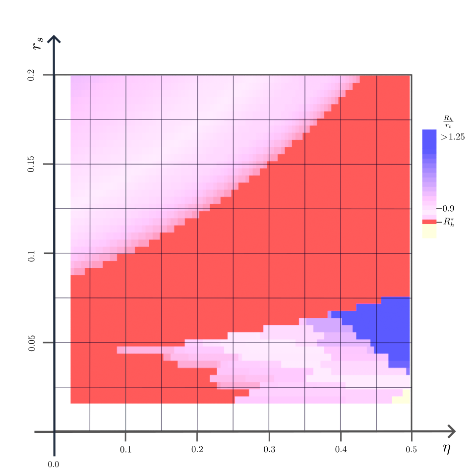
Figure 5: Phase diagram of periodic tight helices with edge length $e=0.25$. The diagram is a reproduction of figure 3 of [15] which was computed numerically over a smooth curve. The diagram shows three main regions, a slightly unwound helix is proferred for larger solvent radii. A thick diagonal stripe of fluids favour the optimal helix. For low solvent radius the helical curve of lowest energy is determined by the packing fraction, with larger packed fractions favouring parallel curves representing the $\beta$–sheet.

Shown in Fig. 5 is a phase–diagram demonstrating the thermodynamic favourable closely packed periodic helical tubes. The helical tube is thought of as immersed in a hard–sphere fluid with packing fraction $\eta$ and relative solvent size $r_{s}$. The helical radius determining the system of least free energy, as compared to all closely packed helices, colours the corresponding square in the phase diagram. Each closely packed helical curve is interpolated using an equilateral polygon of edge length $e=0.25$, in comparison to the open equilateral polygonal curves otherwise considered in this work. Fig. 5 is a reproduction of figure $3$ of [15], differing only in that the original diagram is constructed using smooth curves to define the solute geometry. Both diagrams are in excellent agreement and show three main regions; a thick band of fluid environments for which the optimal helix is thermodynamically most favourable, for larger solvent radii a slightly unwound helix is preferred, for smaller solvent radii the favourability is determined by the packing fraction $\eta$ with higher density fluids favouring the $\beta$–sheet packing. Note the bottom right hand corner is coloured yellow referring to the fully solvated state– a straight tube devoid of any economic packing– this is is not seen in the original diagram and is likely a discretisation artifact.

Since we are interested in short open tubes in this work, we compute the same phase diagram for a tight helical open curves of length $\ell=25$ shown in Fig. 6. The diagram follows the same pattern as the diagram of the periodic helices with the fundamental difference that the $\beta$–sheet structure is not optimal for finite strings.

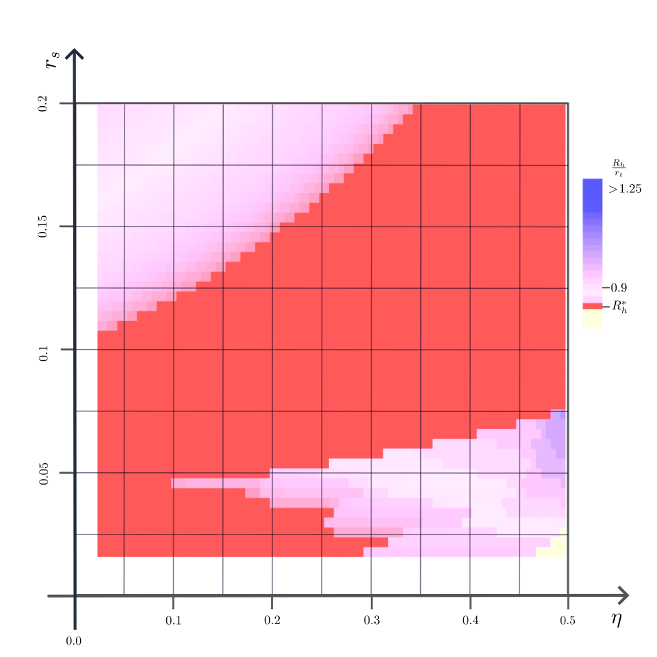
Figure 6: Phase diagram of open tight helices with edge length $e=0.25$ and total length $\ell=25$. The diagram is different to the diagram of the periodic curves (Fig. 5) as the $\beta$–sheet structure is not included. Otherwise the trend between the various regions is quite similar.

The measures of a simple tubular string.

We consider curves given as open equilateral polygons of $n$ vertices and edge length $e$. The curve models the shape of the solute body as the union of $r_{t}$–balls, correspondingly the shape of body bounded by the solvent accessible surface ($\mathcal{B}$) as the union of $(r_{t}+r_{s})$–balls, centered at the vertices $v_{i}$ of the polygonal curve. For a given fluid system the measures (volume, surface area etc.) of the body $\mathcal{B}$ determine the free energy of solvation by (1). The solute is fully solvated if the curve satisfies the simple tube property (condition (2)) for the radius $r=(r_{t}+r_{s})$. This is a geometric condition and does not determine a unique curve shape, referring instead to curves devoid of any economic packing. The energy of the fully solvated state, $\mathbf{F}_{\mathrm{sol}}^{0}$, is a constant depending only upon the geometric parameters of the tubular solute and physical coefficients defining the energy in (1). Very generally, if a curve satisfies the simple tube property for the radius $r$ then the measures of the tubular string are constant depending only on the geometric parameters $n$, $e$ and $r$ and not on the specific shape of the curve. This observation is given in the following proposition. By this one can see that a curve models the solute if the curve satisfies the simple tube property for the radius $r=r_{t}$ since then the volume, i.e. the bulk amount of solute thought as added to the fluid, remains fixed throughout the simulation.

Proposition 0.1 (measures of a simple tube).

The measures of an open equilateral polygonal curve with edge length $e$ and vertex set $\{v_{1},\dots,v_{n}\}$ satisfying condition (2) for ball radius $r$ are given by the following formulas:

$$\begin{array}[]{rcl}\mathrm{V}\left(\bigcup\limits_{i=1}^{n}\mathrm{B}_{r}(v_{i})\right)&=&\pi(n-1)\left(r^{2}e-\frac{e^{3}}{12}\right)+\frac{4\pi}{3}r^{3}\\[16.0pt] \mathrm{A}\left(\bigcup\limits_{i=1}^{n}\mathrm{B}_{r}(v_{i})\right)&=&2(n-1)\pi re+4\pi r^{2}\\[16.0pt] \mathrm{C}\left(\bigcup\limits_{i=1}^{n}\mathrm{B}_{r}(v_{i})\right)&=&2(n-1)\pi\left(e-\sqrt{r^{2}-\left(\frac{e}{2}\right)^{2}}\left(\frac{\pi}{2}-\arccos\left(\frac{e}{2r}\right)\right)\right)+4\pi r\\[16.0pt] \mathrm{X}\left(\bigcup\limits_{i=1}^{n}\mathrm{B}_{r}(v_{i})\right)&=&4\pi\,.\end{array}$$

Proof.

The Voronoi diagram intersected with the ball $\mathrm{B}_{r}(v_{i})$ for each $i$ is a decomposition of the union of balls which, by (2), is disjoint up to a planar face interior to the union of balls. A set belonging to such a decomposition is coloured blue in Fig 7. The volume of this region (blue) corresponding to the string interior vertices $v_{2},\dots,v_{n-1}$ is the volume of a ball without the volume enclosed by two spherical caps and the bounding planes (shaded grey); that is

$$\frac{4\pi}{3}-\frac{2\pi}{3}\left(r-\tfrac{e}{2}\right)^{2}\left(2r-\tfrac{e}{2}\right)=\pi(r^{2}-\frac{e^{3}}{12})\,.$$

The tubular string is the concatenation of $(n-2)$ such regions (blue). The volume of the regions corresponding to the $i=1$ and $i=n$ vertices is the volume of the ball without the volume enclosed by one spherical cap and a bounding plane; so that the addition of both of these volumes is

$$2\frac{4\pi}{3}-\frac{2\pi}{3}\left(r-\tfrac{e}{2}\right)^{2}\left(2r-\tfrac{e}{2}\right)=\frac{4\pi}{3}+\pi(r^{2}-\frac{e^{3}}{12})\,.$$

In sum this gives the computed volume as in the proposition.

Completely analogously the (exposed) surface area of the region (blue) corresponding to the string interior vertices $v_{2},\dots,v_{n-1}$ is the area of the ball without the area of two spherical caps; that is

$$4\pi r^{2}-4\pi r\left(r-\tfrac{e}{2}\right)=2\pi re\,.$$

The total surface area of the tubular string is the area of $(n-2)$ such regions and the surface area of both regions corresponding the $i=1$ and $i=n$ vertices, which sum as

$$8\pi r^{2}-4\pi r\left(r-\tfrac{e}{2}\right)=4\pi r^{2}+2\pi re\,.$$

In total this gives the computed surface area as in the proposition.

The integrated mean curvature measure has a term which is computed over the regular surface of the the union of balls and a term computed over the intersection curves between adjacent balls. Since both principal curvatures are equal to $\frac{1}{r}$ the contribution to the integrated mean curvature from integration over the regular surface is

$$4\pi r+(n-1)2\pi e\,.$$

The contribution to the integrated mean curvature measure computed over the intersection curves between adjacent balls is (minus) half the angle between the normal vectors to intersecting surfaces, $\theta$, integrated along the intersection curve $\gamma$; that is

$$-\oint\limits_{\gamma}\frac{\theta}{2}\,.$$

By symmetry the angle $\theta$ is constant along the intersection curve $\gamma$ and equal to

$$\pi-2\arccos\left(\frac{e}{2r}\right)\,.$$ (4)

The length of the intersection curve $\gamma$ between two arbitrary adjacent balls is

$$2\pi\sqrt{r^{2}-(\tfrac{e}{2})^{2}}\,.$$

There are $(n-1)$ such intersection curves contained in the boundary of the tubular string. In total these contributions give the computed mean curvature term as in the proposition.

The integrated Gaussian curvature is computed via the Euler characteristic and observing that condition (2) ensures that the tubular string has the topology of a ball. ∎

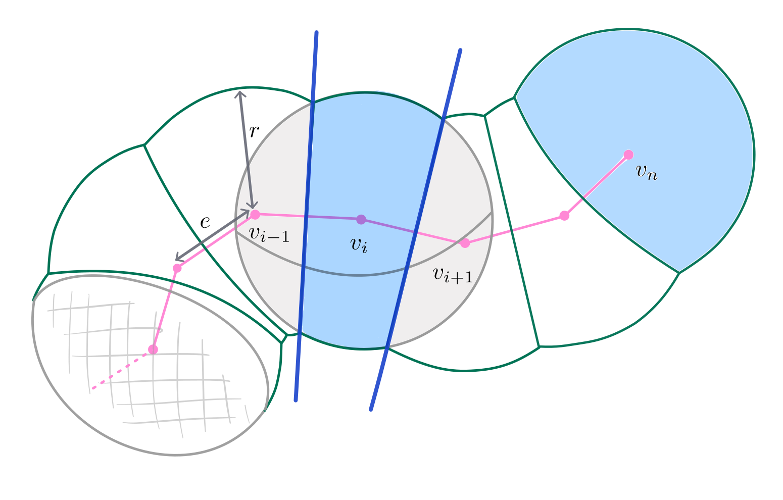
Figure 7: The figure depicts part of the body $\mathcal{B}$, here given as the union of $r$ balls centered along the vertices of an equilateral polygonal curve with $n$ vertices and edge length $e$. In this configuration, the curve satisfies the simple tube property for the radius $r$, condition (2). To compute the measures of the union of balls a disjoint decomposition of $\mathcal{B}$ is used. Such a disjoint decomposition is found by intersecting the $i$^th region of the the Voronoi diagram of the vertex set $\{v_{1},\dots,v_{n}\}$ with the ball $\mathrm{B}_{r}(v_{i})$. Shaded blue is an example of such a set for the interior vertices $\{v_{2},\dots,v_{n-1}\}$ and an example of such a set for end vertices $v_{1},v_{n}$. Each such set is the ball $\mathrm{B}_{r}(v_{i})$ contained in the half space defined by the perpendicular bisecting planes (depicted as dark blue lines) of the incident edges to the vertex.

References

- [1] Z. Ashbridge et al. “Knotting matters: orderly molecular entanglements” In Chem. Soc. Rev. 51, 2022, pp. 7779–7809 DOI: 10.1039/d2cs00323f
- [2] P. Ball “Water as an Active Constituent in Cell Biology” In Chem. Rev. 108.1, 2008, pp. 74–108 DOI: https://doi.org/10.1021/cr068037a
- [3] T. Brouns et al. “Free Energy Landscape and Dynamics of Supercoiled DNA by High-Speed Atomic Force Microscopy” In ACS Nano 12.12, 2018, pp. 11907–11916 DOI: 10.1021/acsnano.8b06994
- [4] J. Cantarella, R.. Kusner and J.. Sullivan “On the minimum ropelength of knots and links” In J. Invent. Math. 150.2, 2002, pp. 257–286 DOI: 10.1007/s00222-002-0234-y
- [5] R. Coles “disSolve” In GitHub repository GitHub, https://github.com/rhocoles/disSolve.git, 2024
- [6] M. Dobson “Protein Folding and Misfolding” In Nature 426, 2003, pp. 884–890 DOI: 10.1038/nature02261
- [7] H. Edelsbrunner “The Union of Balls and Its Dual Shape” In Discrete Comput. Geom. 13.3, 1995, pp. 415–440 DOI: 10.1007/BF02574053
- [8] H. Edelsbrunner and P. Koehl “The Geometry of Biomolecular Solvation” In Combinatorial and Computational Geometry 52, MSRI Book Series Cambridge University Press, 2005, pp. 243–275
- [9] D. Eisenberg and A.. McLachlan “Solvation Energy in Protein Folding and Binding” In Nature 319, 1986, pp. 199–203 DOI: https://doi.org/10.1038/319199a0
- [10] M.. Evans and R. Roth “Shaping the Skin: The Interplay of Mesoscale Geometry and Corneocyte Swelling” In Phys. Rev. Lett. 112.3, 2014, pp. 038102 DOI: 10.1103/PhysRevLett.112.038102
- [11] O. Gonzalez and J.. Maddocks “Global curvature, thickness, and the ideal shapes of knots” In Proc. Natl. Acad. Sci. USA 96.9, 1999, pp. 4769–4773 DOI: 10.1073/pnas.96.9.4769
- [12] Paul Grandgeorge et al. “Mechanics of two filaments in tight orthogonal contact” In Proceedings of the National Academy of Sciences 118.15, 2021, pp. e2021684118 DOI: 10.1073/pnas.2021684118
- [13] H. Hadwiger “Vorlesungen Über Inhalt, Geometrie, Oberfläche und Isoperimetrie” 93, Die Grundlehren der Mathematischen Wissenschaften Springer-Verlag Berlin Heidelberg, 1957 DOI: http://dx.doi.org/10.1007/978-3-642-94702-5
- [14] H. Hansen-Goos and R. Roth “Density functional theory for hard–sphere mixtures: The White Bear version mark II” In J. Phys.: Condens. Matter 18, 2006, pp. 8413–8425 DOI: 10.1088/0953-8984/18/37/002
- [15] H. Hansen-Goos, R. Roth, K. Mecke and S. Dietrich “Solvation of Proteins: Linking Thermodynamics to Geometry” In Phys. Rev. Lett. 99 American Physical Society, 2007, pp. 128101 DOI: 10.1103/PhysRevLett.99.128101
- [16] Yuichi Harano, Roland Roth and Shuntaro Chiba “A morphometric approach for the accurate solvation thermodynamics of proteins and ligands” In Journal of Computational Chemistry 34.23, 2013, pp. 1969–1974 DOI: https://doi.org/10.1002/jcc.23348
- [17] R. Irobalieva, J. Fogg, D. Catanese and al. “Structural diversity of supercoiled DNA” In Nat Commun 6, 2015, pp. 8440 DOI: https://doi.org/10.1038/ncomms9440
- [18] Paul Johanns et al. “The shapes of physical trefoil knots” In Extreme Mechanics Letters 43, 2021, pp. 101172 DOI: https://doi.org/10.1016/j.eml.2021.101172
- [19] I.. Kaltashov and C. Fenselau “Stability of secondary structural elements in a solvent–free environment: the alpha Helix” In Proteins 27.2, 1997, pp. 165–170 DOI: 10.1002/(sici)1097-0134(199702)27:2¡165::aid-prot2¿3.0.co;2-f
- [20] O. Kasper and J. Bohr “The generic geometry of helices and their close-packed structures” In Theor. Chem. Acc 125, 2009, pp. 207–215 DOI: 0.1007/s00214-009-0639-4
- [21] Vsevolod Katritch et al. “Geometry and physics of knots” In Nature 384.6605, 1996, pp. 142–145 DOI: 10.1038/384142a0
- [22] K.. Klenin, F. Tristram, T. Strunk and W. Wenzel “Derivatives of Molecular Surface Area and Volume: Simple and Exact Analytical Formulas” In J. Comput. Chem. 32, 2011, pp. 2647–2653 DOI: 10.1002/jcc.21844
- [23] P.. König, R. Roth and K.. Mecke “Morphological Thermodynamics of Fluids: Shape Dependence of Free Energies” In Phys. Rev. Lett. 93.16, 2004, pp. 160601 DOI: 10.1103/PhysRevLett.93.160601
- [24] B. Lee and F.. Richards “The Interpretation of Protein Structures: Estimation of Static Accessibility” In J. Mol. Biol. 55.3, 1971, pp. 379–400 DOI: https://doi.org/10.1016/0022-2836(71)90324-X
- [25] R.. Litherland, J. Simon, O. Durumeric and E. Rawdon “Thickness of knots” In Topol. Appl. 91.3, 1999, pp. 233–244 DOI: 10.1016/S0166-8641(97)00210-1
- [26] J. Lou and J. Reinitz “Parallel simulated annealing using an adaptive resampling interval” In Parallel Computing 53, 2016, pp. 23–31 DOI: 10.1016/j.parco.2016.02.001
- [27] K. Lum, D. Chandler and J.. Weeks “Hydrophobicity at Small and Large Length Scales” In J. Phys. Chem. B. 103.22, 1990, pp. 4570–4577 DOI: https://doi.org/10.1021/jp984327m
- [28] Zähle M. “Integral and Current Representation of Federer’s Curvature Measures” In Arch. Math 44, 1986, pp. 557–567 DOI: https://doi.org/10.1007/BF01195026
- [29] S. Majumder, M. Marenz, S. Paul and W. Janke “Knots are Generic Stable Phases in Semiflexible Polymers” In Macromolecules 54.12, 2021, pp. 5321–5334 DOI: 10.1021/acs.macromol.0c02584
- [30] Davide Marenduzzo et al. “DNA–DNA interactions in bacteriophage capsids are responsible for the observed DNA knotting” In Proceedings of the National Academy of Sciences 106.52, 2009, pp. 22269–22274 DOI: 10.1073/pnas.0907524106
- [31] M. Marenz and W. Janke “Knots as a Topological Order Parameter for Semiflexible Polymers” In Phys. Rev. Lett. 116, 2016, pp. 128301 DOI: 10.1103/PhysRevLett.116.128301
- [32] A. Maritan, C. Micheletti, A. Trovato and Banavar J. R. “Optimal Shapes of Compact Strings.” In Nature 406, 2000, pp. 287–290 DOI: https://doi.org/10.1038/35018538
- [33] K R Mecke “A morphological model for complex fluids” In Journal of Physics: Condensed Matter 8.47, 1996, pp. 9663 DOI: 10.1088/0953-8984/8/47/080
- [34] K. Millett and E .J. Rawdon “Energy, ropelength, and other physical aspects of equilateral knots” In J. C. P. 186.2, 2003, pp. 426–456 DOI: 10.1016/S0021-9991(03)00026-3
- [35] D.. Naiman and H.. Wynn “Inclusion–Exclusion–Bonferroni Identities and Inequalities for Discrete Tube–Like Problems via Euler Characteristics” In Ann. Statist. 20.1, 1992, pp. 43–76 DOI: 10.1214/aos/1176348512
- [36] A.. Onufriev and D.. Case “Generalized Born Implicit Solvent Models for Biomolecules.” In Annu Rev Biophys. 48, 2019, pp. 275–296 DOI: 10.1146/annurev-biophys-052118-115325
- [37] A.. Onufriev and S. Izadi “Water models for biomolecular simulations” In WIREs Comp. Mol. Sci 8.2, 2018, pp. e1347 DOI: 10.1002/wcms.1347
- [38] T Ooi, M Oobatake, G Némethy and HA Scheraga “Accessible surface areas as a measure of the thermodynamic parameters of hydration of peptides” In Proceedings of the National Academy of Sciences of the United States of America 84.10, 1987, pp. 3086–3090 DOI: 10.1073/pnas.84.10.3086
- [39] P.L. Privalov and C. Crane-Robinson “Role of water in the formation of macromolecular structures” In Eur, Biophys, J. 46, 2017, pp. 203–224 DOI: https://doi.org/10.1007/s00249-016-1161-y
- [40] S. Przybył and P. Pierański “Helical close packings of ideal ropes” In Eur. Phys. J. E Soft Matter 4, 2001, pp. 445–449 DOI: 10.1007/s101890170099
- [41] E.. Rawdon “Can Computers Discover Ideal Knots?” In Experiment. Math. 12.3, 2003, pp. 287–302 DOI: 10.1080/10586458.2003.10504499
- [42] R. Roth, Y. Harano and M. Kinoshita “Morphometric Approach to the Solvation Free Energy of Complex Molecules” In Phys. Rev. Lett. 97.7, 2006, pp. 078101 DOI: 10.1103/PhysRevLett.97.078101
- [43] B Roux and T Simonson “Implicit solvent models” In Biophys. Chem. 78.1-2 Elsevier BV, 1999, pp. 1–20
- [44] G. Salvi and P. De Los Rios “Effective Interactions Cannot Replace Solvent Effects in a Lattice Model of Proteins” In Phys. Rev. Lett. 91.25, 2003, pp. 258102 DOI: 10.1103/PhysRevLett.91.258102
- [45] Eugene Shakhnovich “To knot or not to knot?” In Nature Materials 10.2, 2011, pp. 84–86 DOI: 10.1038/nmat2953
- [46] Thomas Simonson and Axel T. Bruenger “Solvation Free Energies Estimated from Macroscopic Continuum Theory: An Accuracy Assessment” In The Journal of Physical Chemistry 98.17, 1994, pp. 4683–4694 DOI: 10.1021/j100068a033
- [47] Y. Snir and R.. Kamien “Helical Tubes in Crowded Environments” In Phys. Rev. E 75 American Physical Society, 2007, pp. 051114 DOI: 10.1103/PhysRevE.75.051114
- [48] Ivan Spirandelli, Rhoslyn Coles, Gero Friesecke and Myfanwy E. Evans “Exotic self-assembly of hard spheres in a morphometric solvent” In Proceedings of the National Academy of Sciences 121.15, 2024, pp. e2314959121 DOI: 10.1073/pnas.2314959121
- [49] A. Stasiak et al. “Electrophoretic mobility of DNA knots” In Nature 384.6605, 1996, pp. 122 DOI: 10.1038/384122a0
- [50] J.. Sułkowska “On folding of entangled proteins: knots, lassos, links and theta–curves” In Curr. Opin. Struct. Biol. 60, 2020, pp. 131–141 DOI: 10.1016/j.sbi.2020.01.007
- [51] “Topological Polymer Chemistry” Springer Nature Singapore, 2022 DOI: 10.1007/978-981-16-6807-4
- [52] Y. and J.. “Water Mediation in Protein Folding and Molecular Recognition” In Annu. Rev. Biophys. Biomol. Struct. 35, 2006, pp. 389–415 DOI: 10.1146/ annurev.biophys.35.040405.102134