Effective Field Theory Calculation of LIGO-like Compton Scattering and Experiment Proposal for Graviton Detection

Abstract

Despite the lack of a universally accepted quantum gravity theory, gravitons are considered the quantum noise in gravitational waves. Wave mediation requires that gravitons be in a coherence state, with an abundance number of order $\sim 10^{79}$. Thus, the detection of coherent-state gravitons may be possible in a LIGO-like experiment via Compton scattering with a nanospherical test mass. This work presents the associating scattering amplitude calculation using effective field theory, calculating a total cross section approximately $100~\mathrm{cm^{2}}$ for a coherence state and $\sim 10^{-81}~\mathrm{m^{2}}$ for a single graviton. An experiment proposal involving levitation techniques of a nanosphere is given in full description.

1 Introduction

Since 2015, gravitational waves (GWs) are detectable via laser interferometry at the LIGO-Virgo-KAGRA (LVK) observatories [1, 2, 3, 4, 5, 6, 7, 8]. The detection of GW150914 [1] was made possible by measuring the fluctuations in the displacement of hanging-mass reflective mirrors at the LIGO laser interferometer, which are caused by the passing GWs from the source binary black hole merger. These fluctuations, on the order of $\Delta L\sim 10^{-18}$ m (corresponding to a strain of $h\equiv\Delta L/L\sim 10^{-21}$, given the length of the interferometer’s arms of $L\sim 4$ km), are detected by comparing the arm lengths of the interferometer and measuring the shift in the laser light interference pattern as the GW passes through the system. Due to quantum nondemolition, the hanging masses behave like quantum objects, allowing them to detect these miniscule displacements without disturbing the quantum state of the system. The motion of these mirrors, influenced by the GWs, is akin to Brownian motion, where random displacement fluctuations occur due to both the gravitational wave signal and the background noise.

Despite the lack of a widely accepted quantum theory of gravity, GW detection has strengthened the argument for a quantum-classical correspondence between GWs and bosonic gravitons. Gravitons are hypothetical particles that mediate gravitational interactions, and are thus considered the quantum counterpart to GWs and the quantum noise between two gravitational masses [3, 9, 10, 11, 12]. The connection between wave-particle duality and quantum noise was applied to an ideal coalescing binary in Ref. [13], where the astrophysical process of GW formation was mirrored by the Bose-Einstein statistical mechanics of stochastic gravitons in a contracting volume. The entropy of this graviton gas is not induced by the temperature of the system-background ensemble (with $T\sim 1\mathrm{K}$ [10, 11]), but rather by excitations arising from gravitational attraction and high-energy graviton-graviton scatterings [14, 15, 16, 17, 18, 19]. As a result, GW formation throughout coalescence can be idealized as the Brownian motion of gravitons.

A stochastic framework for quantum gravity was introduced in 1996 [21], which offers an alternative to string theory and the canonical Hamiltonian formalism underlying loop quantum gravity. In this framework, the quantum fluctuations in Minkowski spacetime are proposed to cause fluctuations in the gravitational constant, introducing a stochastic correction: $G\rightarrow G+\sigma\xi_{x}$. This modification expands the Einstein field equations (EFEs), so that the core equation incorporates an additive off-equilibrium perturbation factor: $G_{\mu\nu}=8\pi(GT_{\mu\nu}+\sigma\xi_{x}T_{\mu\nu})$, with $c=1$. This expansion is analogous to the linearization of the metric $g_{\mu\nu}$, adding first-order perturbations to the Minkowski metric (i.e., $g_{\mu\nu}=\eta_{\mu\nu}+h_{\mu\nu}$), as well as the linearization of the energy-momentum tensor for an imperfect fluid [23]: $T_{\mu\nu}=T^{(0)}_{\mu\nu}+\pi_{\mu\nu}$. This inclusion of stochastic corrections in the EFEs leads to corresponding Langevin [22] and Fokker-Planck [21] equations, which describe first-order metric pertubations as quantum fluctuations (i.e., graviton signatures). These fluctuations, arising from quantum gravitational effects within a contracting volume from inspiral to the chirp phase of coalescence, were analyzed in Ref. [20].

If gravitons are emitted during the chirp phase of GW emission, they must be in a coherent state [9, 10, 11], with the number of gravitons scaled as $\mathrm{N}\propto\mathcal{M}/f_{\mathrm{GW}}$ [13], with $\hbar=1$. Here, $\mathcal{M}=(m_{1}m_{2})^{3/5}/(m_{1}+m_{2})^{1/5}$ is the chirp mass of the source binary and $f_{\mathrm{GW}}$ is the GW frequency upon observation. This frequency is expected to correspond the frequency at the chirp phase, assuming negligable wave dampening. E.g., for GW150914 with a source chirp mass of $\mathcal{M}\sim 28M_{\odot}$ and a frequency of $f_{\mathrm{GW}}\sim 200$ Hz [1], the number of gravitons in a coherent state is estimated to be $\mathrm{N}\approx 4.5\times 10^{79}$ (also obtained in Ref. [24]). In a coherent state, the thermal noise between individual gravitons are minimal due to the low temperature of the universe’s vacuum ($T\sim 1$ K), which leads to minimal random fluctuations within the GW. This minimal thermal noise ensures that the wave phases remain unshifted, perserving the coherence of the GW signal throughout its propagation.

By treating the $\mathrm{N}$ coherent-state gravitons as a single condensed graviton, a Compton scattering event with a nanospherical test mass can be observed. However, this is possible only under the condition that the nanosphere is not influenced by thermal noise or by the zero-point energy influenced by the position-momentum uncertainty principle. In the presence of these factors, any interaction with the coherent-state gravitons would be suppressed, given the relative weakness of gravitational interactions. The effective field theory (EFT) gravitational gauge coupling, $\kappa=\sqrt{8\pi G}$, describes this interaction [16, 17, 18, 19]. This study calculates the corresponding scattering amplitude using EFT, which allows for the determination of the relevant cross section of GW-nanoparticle interaction. The proposed Compton-like experiment builds upon earlier work in Ref. [24]. By reducing the effects of thermal noise and zero-point energy, only the Brownian motion of the nanosphere due to interaction with the coherent-state gravitons will be detected. This event deduces the observation of coherent-state gravitons in a GW.

2 Methods in Effective Field Theory

2.1 Governing Equations and Gauges

The Lagrangian of a gravitational interaction involving scalar particles contains the individidual Lagrangian for the scalar particles and the Einstein-Hilbert Lagrangian:

$$\mathcal{L}=\mathcal{L}_{\mathrm{Scalar}}+\mathcal{L}_{\mathrm{EH}}.$$ (1)

In Minkowski spacetime, scalar particles governed by the field $\phi$ follow the Lagrangian

$$\mathcal{L}_{\mathrm{Scalar}}=\frac{1}{2}(\partial_{\mu}\phi)(\partial^{\mu}\phi)-\frac{1}{2}m^{2}\phi^{2},$$ (2)

where $m$ is the mass of the scalar particle. Applying this Lagrangian to the Euler-Lagrange equation yields the Klein-Gordon equation as the corresponding equation of motion:

$$(\partial_{\mu}\partial^{\mu}-m^{2})\phi=0,$$ (3)

where $\partial_{\mu}\partial^{\mu}\equiv\eta_{\mu\nu}\partial^{\mu}\partial^{\nu}$ defines the d’Alembert wave operator $\Box\equiv\partial^{2}_{t}-\nabla^{2}$, using the metric signature $\eta_{\mu\nu}=\mathrm{diag}(+,-,-,-)$. This scalar field has a plane wave solution that satisfies orthonormality $\langle\phi_{i}|\phi_{j}\rangle=\delta_{ij}$.

For gravitational field expressed by the EFEs, the Einstein-Hilbert Lagrangian governs the dynamics:

$$\mathcal{L}_{\mathrm{EH}}=-\frac{1}{16\pi G}R,$$ (4)

where $R\equiv g^{\mu\nu}R_{\mu\nu}$ is the Ricci scalar, the trace of the Ricci curvature tensor. In flat spacetime ($g_{\mu\nu}=\eta_{\mu\nu}$), $\mathcal{L}_{\mathrm{EH}}=0$ since $R=0$. However, given a linearized metric $g_{\mu\nu}=\eta_{\mu\nu}+h_{\mu\nu}$, the Ricci scalar depends on the pertubation: $R=h^{\mu\nu}R_{\mu\nu}$. Under harmonic coordinates, Lemma 3.32 in Ref. [25] is used to express the Ricci tensor $R_{\mu\nu}$ in terms of the Laplace-Beltrami operator:

$$R_{\mu\nu}=-\frac{1}{2}\Delta^{\mathrm{LB}}g_{\mu\nu},~~~\mathrm{where}~~~\Delta^{\mathrm{LB}}=\frac{1}{\sqrt{|g|}}\partial_{\alpha}\left(\sqrt{|g|}g^{\alpha\beta}\partial_{\beta}\right).$$ (5)

For a linearized metric, its determinant is approximately unitary: $|g|\approx 1$; this writes Eq. (4) as

$$\begin{split}&0=-\frac{1}{16\pi G}h^{\mu\nu}\left\{-\frac{1}{2}\partial_{\alpha}\left[\left(\eta^{\alpha\beta}+h^{\alpha\beta}\right)\partial_{\beta}\right]\left(\eta_{\mu\nu}+h_{\mu\nu}\right)\right\}.\end{split}$$ (6)

The bracket terms in Eq. (6) can be further reduced into a wave equation of a free graviton. Simplifying terms involving $h_{\mu\nu}$ and neglecting second-order perturbations $\mathcal{O}(h^{2})$, the free wave equation and its plane wave solution are

$$\Box h_{\mu\nu}=0~~~\rightarrow~~~h_{\mu\nu}(x)\propto\exp\left(-ip_{\rho}x^{\rho}\right)\varepsilon_{\mu\nu}(p).$$ (7)

Here, $\varepsilon_{\mu\nu}(p)$ is the polarization tensor, and $p^{\mu}=(E,\vec{p}\,)$ is the 4-momentum. Since $h_{\mu\nu}$ is a rank-2 tensor, the graviton has spin $s=2$. A massless graviton, however, has only two degrees of freedom (d.o.f); this corresponds to the two orthogonal polarization states of a propagating GW. Thus, massless gravitons have the traceless and transverse (TT) gauge that GWs have, which defines

$$\varepsilon_{\mu\nu}^{\mathrm{TT}}(p)=\left(\begin{array}[]{cccc}0&0&0&0\\ 0&h_{+}&h_{\times}&0\\ 0&h_{\times}&-h_{+}&0\\ 0&0&0&0\end{array}\right).$$ (8)

Furthermore, the TT-gauge sets the conditions $\varepsilon_{\mu\nu}^{\mathrm{TT}}\eta^{\mu\nu}=0$ and $\varepsilon_{\mu\nu}^{\mathrm{TT}}p^{\mu}=\varepsilon_{\mu\nu}^{\mathrm{TT}}p^{\nu}=0$. TT-gauge properties will prove to be instrumental in the EFE-based calculations of the Compton scattering cross section.

The equation of motion for free gravitons, Eq. (7), allows us to derive the graviton’s Lagrangian using the Euler-Lagrange equation. As provided in Ref. [16], the Lagrangian of a graviton with a tensor field $h_{\mu\nu}$ is given by

$$\begin{split}\mathcal{L}_{\mathrm{Graviton}}=\frac{1}{2}(\partial_{\alpha}h^{\mu\nu})(\partial^{\alpha}h_{\mu\nu})-\frac{1}{4}(\partial_{\alpha}h_{\mu}^{~\mu})(\partial^{\alpha}h_{\nu}^{~\nu}).\end{split}$$ (9)

The first term describes the kinetic energy, and the second term ensures gauge invariance. For TT-gauged gravitons with the field $h^{\mathrm{TT}}_{\mu\nu}$, the traceless condition yields $h_{\mu}^{~\mu}=h_{\nu}^{~\nu}=0$.

2.2 Feynman Rules

As the Einstein-Hilbert Lagrangian has 10 d.o.f.’s, and the TT-gauged graviton has only two, a discrepancy in the d.o.f.’s arises. This is resolved by introducing ghost fields to fix the gauge [15, 16]. This ensures that only the physically relevant d.o.f’s contribute, reducing the Einstein-Hilbert Lagrangian to match the graviton Lagrangian. A parameter $\epsilon$ is introduced as part of this procedure to account for these adjustments [15, 16].

In a Compton-like scattering process involving a scalar particle and coherent-state gravitons (the GW), scalar particles act as exchange particles. In corresponding Feynman diagrams, the scalar propagator incorporates the parameter $\epsilon$ to ensure proper convergence and causality:

$$S=\int\frac{d^{4}q}{(2\pi)^{4}}\frac{i}{q^{2}-m^{2}+i\epsilon},$$ (10)

where $q$ is the internal 4-momentum between the vertices. The parameter $\epsilon$ also ensures that the propagator remains well-defined, particularly near the mass-shell condition $q^{2}=m^{2}$. From this point on, unless otherwise specified, spacetime indices of 4-momenta are omitted for simplicity. 4-momentum is labeled as $p_{i}$, and the 3-momentum component is denoted $\vec{p}_{i}$. Once the total amplitude squared $|\mathcal{A}_{\mathrm{tot}}|^{2}$ is determined to compute observables (e.g., differential cross sections, $d\sigma\propto|\mathcal{A}_{\mathrm{tot}}|^{2}dt$), a Taylor expansion for small $\epsilon$ is performed. This approach yields convergent, $\epsilon$-independent principle values, ensuring consistency with physical predictions.

The Feynman rules for scalar- and graviton-graviton scattering diagrams are provided in Refs. [15, 16]. For Compton scattering, the relevant diagrams in the center of momentum (CM) frame include the $t$- and $s$-channel diagrams shown in Figure 1. In these diagrams, the TT-gauged graviton and scalar lines represent the external particles, with a scalar line serving as the propagator. This framework models a quantum interpretation of a LIGO-like experiment, illustrating how a GW interacts with a suspended mass. To align with this scenario, it is assumed that the scalar mass remains stationary in the lab frame.

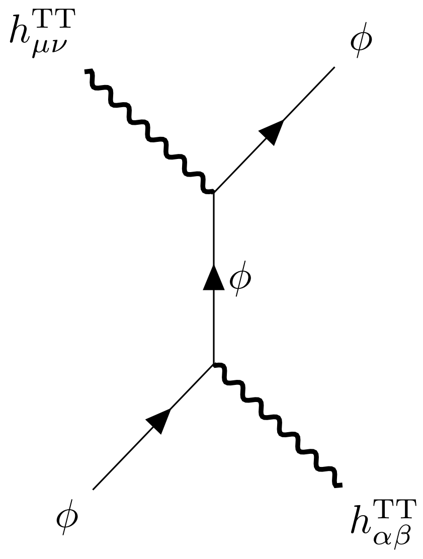
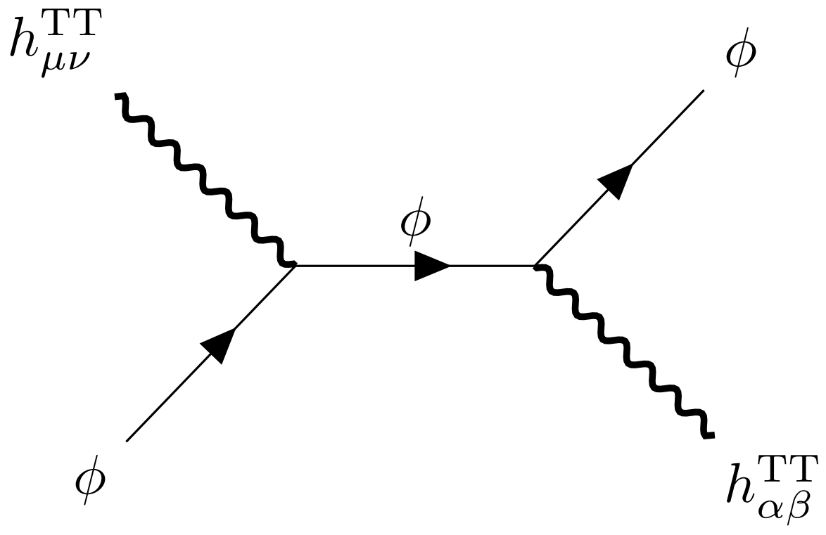
Figure 1: EFT Feynman diagrams of scalar-graviton Compton scattering. (a) a momentum-transfer $t$-channel diagram; (b) a center of momentum $s$-channel diagram.

The Feynman components for scalar-graviton diagrams consist of external scalar and graviton lines (respectively solid arrows and thick wavy lines), and a scalar line between two vertices. Scalar particles are represented by external scalar functions $\phi(p_{i})$ entering the vertex and $\phi^{*}(p_{j})$ leaving the vertex, with their momentum-space propagator given by Eq. (10). TT-gauged gravitons, on the other hand, are described by external polarization tensors $\varepsilon_{\mu\nu}^{\mathrm{TT}}(p_{i})$ entering the vertex and $\varepsilon_{\mu\nu}^{*~\mathrm{TT}}(p_{j})$ exiting the vertex.

Figure 2: A scalar-graviton vertex.

The scalar-graviton vertex, depicted in Figure 2, provides the interaction between a graviton and two scalar particles. The vertex factor in momentum-space, for the given flow of the 4-momenta shown, is given as

$$\begin{split}V^{\mu\nu}=&\,i\kappa\left[(p_{2}^{\mu}p_{3}^{\nu}+p_{3}^{\mu}p_{2}^{\nu})-\eta^{\mu\nu}(p_{2}\cdot p_{3}-m^{2})\right]\\ &\times(2\pi)^{4}\delta^{4}(p_{1}+p_{2}-p_{3}).\end{split}$$ (11)

Here, the spacetime indices of the vertex tensor couple with those of the TT-polarization tensor. The vertex factor depends solely on the scalar particle’s 4-momenta, with one corresponding to the internal momentum. If the direction of the scalar particle’s 4-momentum is flipped, a negative sign is introduced. Similarly, reversing the graviton’s momentum flips the sign on metric term $\eta^{\mu\nu}$.

Because the vertex represents the interaction between one scalar particle and one graviton, the total number of gravitons in the coherent state ($\mathrm{N}$) must be taken into account. This consideration is essential for calculating the total cross section, as $\mathrm{N}$ coherent-state gravitons contribute equally to the scattering process. However, due to the absence of significant dispersion in the interaction, the coherent state behaves collectively as a singular particle. As a result, each vertex is factored by $\mathrm{N}^{1/4}$, leading to $\mathcal{A}_{\mathrm{tot}}\propto\sqrt{\mathrm{N}}$ and $d\sigma\propto\mathrm{N}$. This scaling underscores the coherent amplification of the scattering cross-section by the graviton ensemble rather than the individual contribution of a singular graviton.

3 Calculating $\mathcal{A}_{\mathrm{tot}}$

Using the Feynman rules in Section 2.2, the total amplitude, $\mathcal{A}_{\mathrm{tot}}=\mathcal{A}_{t}+\mathcal{A}_{s}$, is determined using Feynman calculus. This amplitude describes, in the CM frame, the hypothetical scattering of a scalar mass by TT-gauged gravitons in a coherent state, thus acting as a singular graviton. To connect this result with observable phenomena, a transformation into the lab frame – the frame where GWs are detected – is necessary. Given that the GW energy in the lab frame far exceeds the scalar particle’s rest mass, the scalar particle is approximated as effectively massless (i.e., $m=0$) to simplify the analysis.

3.1 $t$-channel Compton scattering

After following the Feynman rules, the amplitude calculation for the $t$-channel in Figure 1 is

$$\begin{split}\mathcal{A}_{t}=&\,\kappa^{2}\sqrt{\mathrm{N}}\frac{\phi^{*}(p_{3})\phi(p_{2})}{t+i\epsilon}\\ &\times\varepsilon^{*~\mathrm{TT}}_{\alpha\beta}(p_{4})\left[(p_{2}^{\alpha}(p_{2}^{\beta}-p_{4}^{\beta})+(p_{2}^{\alpha}-p_{4}^{\alpha})p_{2}^{\beta})+\eta^{\alpha\beta}(p_{2}\cdot(p_{2}-p_{4}))\right]\\ &\times\varepsilon^{\mathrm{TT}}_{\mu\nu}(p_{1})\left[((p_{2}^{\mu}-p_{4}^{\mu})p_{3}^{\nu}+p_{3}^{\mu}(p_{2}^{\nu}-p_{4}^{\nu}))-\eta^{\mu\nu}((p_{2}-p_{4})\cdot p_{3})\right].\end{split}$$ (12)

Here, $t=(p_{2}-p_{4})^{2}=(p_{1}-p_{3})^{2}$ is the Lorentz-invariant momentum transfer. The internal momentum is chosen to flow through the bottom vertex. Since the scalar lines correspond to one particle, the inner product of scalar functions produces unity: $\phi^{*}(p_{3})\phi(p_{2})=1$. Applying the TT gauge to the graviton polarization tensor greatly simplifies the expression:

$$\begin{split}\mathcal{A}_{t}=\frac{2\kappa^{2}\sqrt{\mathrm{N}}}{t+i\epsilon}&~\varepsilon^{*~\mathrm{TT}}_{\alpha\beta}(p_{4})p_{2}^{\alpha}p_{2}^{\beta}\\ &\times\varepsilon^{\mathrm{TT}}_{\mu\nu}(p_{1})\left[p_{3}^{\nu}(p_{2}^{\mu}-p_{4}^{\mu})+p_{3}^{\mu}(p_{2}^{\nu}-p_{4}^{\nu})\right].\end{split}$$ (13)

Because the tensor elements are real, $\varepsilon^{*~\mathrm{TT}}_{\alpha\beta}=\varepsilon^{\mathrm{TT}}_{\alpha\beta}$. The contraction of a TT-polarization tensor with a 4-momentum vector is given by

$$\varepsilon^{\mathrm{TT}}_{\alpha\beta}(p_{b})p_{a}^{\alpha}=\begin{bmatrix}0,&h^{+}_{b}p_{ax}+h^{\times}_{b}p_{ay},&h^{\times}_{b}p_{ax}-h^{+}_{b}p_{ay},&0\end{bmatrix},$$ (14)

subsituting this into the simplifed amplitude yields

$$\begin{split}\mathcal{A}_{t}=&\frac{4\kappa^{2}\sqrt{\mathrm{N}}}{t+i\epsilon}\Big{[}\left(h^{+}_{4}(p^{{}^{\prime}\,2}_{2y}-p^{{}^{\prime}\,2}_{2x})-2h^{\times}_{4}p^{\prime}_{2x}p^{\prime}_{2y}\right)\\ &\times\left((h^{+}_{1}p^{\prime}_{3x}+h^{\times}_{1}p^{\prime}_{3y})(p^{\prime}_{4x}-p^{\prime}_{2x})+(h^{\times}_{1}p^{\prime}_{3x}-h^{+}_{1}p^{\prime}_{3y})(p^{\prime}_{4y}-p^{\prime}_{2y})\right)\Big{]}.\end{split}$$ (15)

We begin to see that the ampltude depends on the TT polarization states and the 3-momentum components of both the scalar particle and the outgoing graviton.

In the CM frame, the incoming and outgoing 3-momenta are equal in magnitude but opposite in direction, reflecting the symmetry of the collision: $\vec{p}\,^{\prime}_{1,3}=-\vec{p}\,^{\prime}_{2,4}$. The scattering from an incoming particle into an outgoing one is described by the scatting angle $\theta$, such that $\vec{p}\,^{\prime}_{1,2}=\vec{p}\,^{\prime}_{3,4}\cos\theta$. Applying these relations to individual components, i.e., $p^{\prime}_{1i,2i}=p^{\prime}_{3i,4i}\cos\theta$ and $p^{\prime}_{1i,3i}=-p^{\prime}_{2i,4i}$, allows the simplification of Eq. (15) in terms of only one 3-momentum, chosen here as the outgoing scalar particle momentum $\vec{p}\,^{\prime}_{3}$:

$$\begin{split}\mathcal{A}_{t}=&\frac{4\kappa^{2}\sqrt{\mathrm{N}}}{t+i\epsilon}\cos^{2}\theta(1-\cos\theta)\\ &\times\Big{[}h^{+}_{4}h^{+}_{1}(p^{{}^{\prime}\,2}_{3y}-p^{{}^{\prime}\,2}_{3x})^{2}+4h^{\times}_{4}h^{\times}_{1}p^{{}^{\prime}\,2}_{3x}p^{{}^{\prime}\,2}_{3y}\\ &~~~~~~-2(p^{{}^{\prime}\,2}_{3y}-p^{{}^{\prime}\,2}_{3x})p^{\prime}_{3x}p^{\prime}_{3y}\left(h^{+}_{4}h^{\times}_{1}+h^{\times}_{4}h^{+}_{1}\right)\Big{]}.\end{split}$$ (16)

In the lab frame, this momentum corresponds to the scalar particle’s motion after interaction with the incoming GW. For massless interacting particles in the CM frame, the relation $\cos\theta=1+2t/s$ applies, where $s=(p_{1}+p_{2})^{2}=(p_{3}+p_{4})^{2}$ is the Lorentz-invariant center-of-momentum energy. In this frame, the magnitude of the 3-momentum is related to $s$ via $s=4|p^{\prime}|^{2}$.

The x- and y-components of $\vec{p}\,^{\prime}_{3}$ construct the transverse momentum $\vec{p}\,^{\prime}_{T}$, expressed in polar coordinates as trigometric functions of a transverse angle $\psi$. Since the transverse plane is independent of the inclination set by the scattering angle $\theta$, integration over all transverse angles is applied to the x- and y-components of $\vec{p}\,^{\prime}_{3}$:

$$\begin{split}&(p^{{}^{\prime}\,2}_{3y}-p^{{}^{\prime}\,2}_{3x})^{2}=|p^{\prime}_{T}|^{4}\int_{0}^{2\pi}(\sin^{2}\psi-\cos^{2}\psi)d\psi=\pi|p^{\prime}_{T}|^{4},\\ &p^{{}^{\prime}\,2}_{3x}p^{{}^{\prime}\,2}_{3y}=|p^{\prime}_{T}|^{4}\int_{0}^{2\pi}(\cos^{2}\psi\,\sin^{2}\psi)d\psi=\frac{\pi}{4}|p^{\prime}_{T}|^{4},\\ &(p^{{}^{\prime}\,2}_{3y}-p^{{}^{\prime}\,2}_{3x})p^{\prime}_{3x}p^{\prime}_{3y}=|p^{\prime}_{T}|^{4}\int_{0}^{2\pi}\left((\sin^{2}\psi-\cos^{2}\psi)\cos\psi\,\sin\psi\right)d\psi=0.\end{split}$$ (17)

With $|p^{\prime}_{T}|=|p^{\prime}|\sin\theta$, the transverse momentum can be rewritten in terms of $t$ and $s$ via $\sin\theta=\sqrt{1-\cos^{2}\theta}$ and the Lorentz-invariant definitions of $\cos\theta$ and $|p^{\prime}|$. Consequently, the $t$-channel amplitude in the CM frame is

$$\begin{split}\mathcal{A}_{t}=-\frac{\pi\kappa^{2}\sqrt{\mathrm{N}}}{4}\frac{s^{2}}{t+i\epsilon}\left(\frac{2t}{s}\right)\left(\frac{2t}{s}+1\right)^{2}\left(\frac{4t^{2}}{s^{2}}+\frac{4t}{s}\right)^{2}\left[h^{+}_{1}h^{+}_{4}+h^{\times}_{1}h^{\times}_{4}\right].\end{split}$$ (18)

3.2 $s$-channel Compton scattering

After following the Feynman rules and applying the TT-gauge, the $s$-channel amplitude shown as Figure 1 is given by

$$\begin{split}\mathcal{A}_{s}=2\kappa^{2}\sqrt{\mathrm{N}}\frac{\phi^{*}(3)\phi(2)}{s+i\epsilon}&~\varepsilon^{\mathrm{TT}}_{\alpha\beta}(p_{4})p_{3}^{\alpha}p_{3}^{\beta}\\ &\times\varepsilon^{\mathrm{TT}}_{\mu\nu}(p_{1})\left[(p_{2}^{\mu}(p_{3}+p_{4})^{\nu}+p_{2}^{\nu}(p_{3}+p_{4})^{\mu})\right].\end{split}$$ (19)

Using the relation in Eq. (14) and applying the CM condition $p^{\prime}_{3i}=-p^{\prime}_{4i}$, the $s$-channel amplitude simplfies to a null result:

$$\begin{split}\mathcal{A}_{s}&=\frac{4\kappa^{2}\sqrt{\mathrm{N}}}{s+i\epsilon}\Big{[}\left(h^{+}_{4}(p^{{}^{\prime}\,2}_{3y}-p^{{}^{\prime}\,2}_{3x})-2h^{\times}_{4}p^{\prime}_{3x}p^{\prime}_{3y}\right)\\ &~\times\left((h^{+}_{1}p^{\prime}_{2x}+h^{\times}_{1}p^{\prime}_{2y})(-p^{\prime}_{3x}-p^{\prime}_{4x})+(h^{\times}_{1}p^{\prime}_{3x}-h^{+}_{1}p^{\prime}_{3y})(-p^{\prime}_{3y}-p^{\prime}_{4y})\right)\Big{]}\\ &=0.\end{split}$$ (20)

3.3 Total Amplitude

Therefore, the total amplitude of scalar-graviton Compton scattering is solely governed by the $t$-channel amplitude. As it is primarily expressed in terms of Lorentz-invariant variables, the transformation into the lab frame only affects the configuration of the plus and cross polarizations. Specifically, the polarizations transform as $h_{1,4}^{+,\times}\rightarrow h_{+,\times}$, which intends to show non-dispersion (or negligably small dispersion) in the lab frame:

$$\begin{split}\implies\mathcal{A}_{\,\mathrm{Lab}}=-\frac{\pi\kappa^{2}\sqrt{\mathrm{N}}}{4}\frac{s^{2}}{t+i\epsilon}\left(\frac{2t}{s}\right)\left(\frac{2t}{s}+1\right)^{2}\left(\frac{4t^{2}}{s^{2}}+\frac{4t}{s}\right)^{2}\left[h_{+}^{2}+h_{\times}^{2}\right].\end{split}$$ (21)

Here, $\left[h_{+}^{2}+h_{\times}^{2}\right]$ is proportional to the energy flux density of monochromatic GWs as the square of the wave’s classical amplitude:

$$\mathcal{F}_{\mathrm{GW}}=\frac{1}{32\pi G}(2\pi f_{\mathrm{GW}})^{2}\left[h_{+}^{2}+h_{\times}^{2}\right].$$ (22)

4 Calculating $\sigma$

After computing the magnitude squared of Eq. (21), defined as $|\mathcal{A}_{\mathrm{tot}}|^{2}=\mathcal{A}^{*}_{\mathrm{tot}}\mathcal{A}_{\mathrm{tot}}$, one can determine the differential cross section with respect to $t$ via the expression

$$\frac{d\sigma}{dt}=\frac{1}{16\pi s^{2}}|\mathcal{A}_{\mathrm{tot}}|^{2}.$$ (23)

To compute $\sigma\equiv\int d\sigma$, the gauge-fixing parameter $\epsilon$ in Eq. (21) must be addressed. Isolating an $\epsilon$-independent principle value requires the Taylor expansion for small $\epsilon$, which is applied to the following integral evaluation:

$$\sigma=\lim_{\epsilon\rightarrow 0}\left[\frac{1}{16\pi s^{2}}\int_{-s}^{0}\mathcal{A}^{*}_{\mathrm{tot}}\mathcal{A}_{\mathrm{tot}}dt\right]\Rightarrow\frac{512\pi}{15015}\mathrm{N}*G^{2}\left[h_{+}^{2}+h_{\times}^{2}\right]^{2}s.$$ (24)

Here, the total cross section is energy-dependent, i.e. dependent on $s$. Therefore, to account for all possible values of $s$ between two massless particles, its average must be evaluated via the distribution functions of the two incoming particles $f(\vec{p}_{1,2})$:

$$\langle s\rangle=\frac{1}{\iint_{-\infty}^{\infty}d^{3}\vec{p}_{1}d^{3}\vec{p}_{2}f(\vec{p}_{1})f(\vec{p}_{2})}\iint_{-\infty}^{\infty}s(\vec{p}_{1},\vec{p}_{2})~d^{3}\vec{p}_{1}d^{3}\vec{p}_{2}f(\vec{p}_{1})f(\vec{p}_{2}).$$ (25)

In the lab frame, ${s}=2|\vec{p}_{1}||\vec{p}_{2}|(1-\cos(\phi_{1}-\phi_{2})\sin\theta_{1}\sin\theta_{2}-\cos\theta_{1}\cos\theta_{2})$, which depends on the particles’ individual projections by the azimuthal and polar angles in their inertial frames.

Particle kinematics in an ensemble of inertial frames are influenced by the system’s entropic setting. For massless particles, $\langle s\rangle$ is proportional to the entropic energy $\Theta$ (typically the thermal energy $k_{B}T$ in thermodynamic contexts). Examples of known quantities of $\langle s\rangle$ include $18\Theta^{2}$ between two Maxwell-Boltzmann particles [26], and $14.5927\Theta^{2}$ between two Bose-Einstein particles, [13]. Between one Maxwell-Boltzmann particle and one Bose-Einstein particle (i.e., the scalar particle and the TT-gauged graviton, respectively), $\langle s\rangle=16.2071\Theta^{2}$. Therefore,

$$\langle\sigma\rangle=0.55265\,{\mathrm{N}}*\pi G^{2}\left[h_{+}^{2}+h_{\times}^{2}\right]^{2}\Theta^{2}.$$ (26)

In a LIGO-like experiment, the hanging mass experiences fluctuations akin to Brownian motion due to its interaction with the propagating GW. This behavior establishes a link between the system’s entropic energy and the GW energy: $\Theta=E_{\mathrm{GW}}$. Using the chirp mass relation to GW energy, $E_{\mathrm{GW}}\simeq 0.11296\mathcal{M}$ [13], we find

$$\begin{split}\langle\sigma\rangle&=0.0624272\,{\mathrm{N}}*\pi G^{2}\mathcal{M}^{2}\left[h_{+}^{2}+h_{\times}^{2}\right]^{2}\\ &\simeq 4\times 10^{-3}{\mathrm{N}}*A_{\mathrm{chirp}}\left[h_{+}^{2}+h_{\times}^{2}\right]^{2},\end{split}$$ (27)

where $A_{\mathrm{chirp}}=16\pi G^{2}\mathcal{M}^{2}$ is the surface area associated with the source chirp mass. For sample values of a chirp mass of order $\sim 10^{31}$ kg, a classical GW amplitude of order $\sim 10^{-22}$, and a total number of coherent-state gravitons $\mathrm{N}$ of order $\sim 10^{79}$, the total cross section of the Compton scattering is approximately $100~\mathrm{cm^{2}}$. In stark contrast, the cross section involving a singular graviton (given the same chirp mass and wave amplitude) is of order $\sim 10^{-81}~\mathrm{m^{2}}$.

5 Discussion

While the Compton scattering between a single graviton and a scalar particle yields a divergent cross section in a low-energy regime [27], this work yields an infinitesimally small cross section utilizing the TT gauge. An infinitesimally small cross section was also obtained in Ref. [28] as $\sim 10^{-70}~\mathrm{m^{2}}$ via the scaling of the Planck length squared ($l_{\mathrm{P}}^{2}\equiv G\hbar/c^{3}$ in SI units). In both cases, regardless, these calculations show that singular graviton detection is physically impossible. However, the coherent-state nature of gravitons in a GW fundamentally alters this scenario, producing a measurable cross section of $100~\mathrm{cm^{2}}$. A feasibly measurable cross section using coherent-state gravitons was obtained in Ref. [28] as $\sim 10^{8}~\mathrm{m^{2}}$.

The $100~\mathrm{cm^{2}}$ result arises from the $t$-channel diagram, which involves an asymmetic momentum transfer in the CM frame that keeps the calculation non-zero. The secondary $s$-channel diagram entails symmetric incoming/outgoing momenta that nullifies the associating amplitude. Therefore, the asymmetry inherent in the $t$-channel momentum transfer enables a non-zero scattering amplitude, indicating that coherent-state, TT-gauged gravitons can interact with a scalar particle.

Unlike individual gravitons, whose miniscule cross sections render their detection practically impossible, the coherenc state amplifies the scattering cross section to a macroscopically measurable scale. This collective behavior not only makes graviton detection experiments feasible but also reinforces the potential of GW observatories like LIGO to probe fundamental aspects of quantum gravity and test the coherence properties of gravitons.

5.1 Experiment Proposal

If a coherent state of $\mathrm{N}$ gravitons behaves collectively as a single condensed graviton, its Compton-like scattering with a nanospherical test mass could become measurable, given the calculated 100 $\mathrm{cm^{2}}$ total cross section. However, detecting such scattering events requires carefully controlled experimental conditions to mitigate thermal noise and quantum mechanical zero-point energy.

Thermal noise can be minimized by operating in a highly evacuated environment cooled to milikelvin temperatures, effectively suppressing thermal excitations. At these temperatures, however, quantum mechanical zero-point energy introduces position uncertainty for the nanosphere. This uncertainty can be constrained using levitation techniques, usch as magnetic field stabilization or optical trapping, to achieve stable suspension of the nanosphere. These levitation methods aim to replicate, at a nanoscale, the functiona behavior of a suspended mass in inferometric detectors like LIGO. In this setup, Brownian-like motion of the levitated nanosphere can serve as a proxy for interactions with coherent-state gravitons propagating in a GW.

Stable magnetic levitation of nanospheres has been studied both theoretically [29] and experimentally [30, 31, 32, 33, 34]. The theoretical work demonstrated that nanospheres with uniaxial anisotropy can achieve stable levitation in a Ioffe-Pritchard magnetic field through quantum spin stabilization. Experimentally, paramagnetic solutions, such as aqueous $\mathrm{MnCl_{2}}$ at various concentrations, have been used as a medium to levitate test particles (e.g. glass beads and silver particles in micron, nanopowder, and nanocolloid forms [34]). Although these experiments were conducted at room temperature, the combined factors of paramagnetic media and magnetic anisotropies could potentially reduce the sensitivity required to detect gravitons, by dampening the Brownian-like motion of the levitated nanosphere.

Optical levitation provides an alternative that is free from the constraints of magnetic anistropies or levitation media [35, 36, 37, 38]. By using focused laser beams, nanospheres can be trapped in an optical potential, eliminating the need for external magnetic fields. Cooling the system to near absolute zero drives the nanosphere to its quantum ground state, providing a robust stabilization mechanism [35, 38]. This approach would be advantagous for creating a highly sensitive detection apparatus capable of observing interactions with coherent-state gravitons, which may manifest as off-equilibirum fluctuations.

These levitation practices should be done in the proximity of the LVK observatories, to ensure a sanity check that a propagating GW has been detected in the macroscopic scale.

6 Conclusion

As it is possible to detect GWs using interferometry, the nanoscopic recreation of a LIGO-like experiment entails measuring the Compton scattering between a nanosphere and coherent-state gravitons that propogate in the GW. The essential parameter of detecting such scattering events is the cross section, which is obtainable when utilizing EFT Feynam calculus to calculate the scattering amplitude in the center-of-momentum frame. Transformation in the lab frame yields an associating scattering amplitude that is used to find the cross section. It is found that the coherence nature of GWs amplifies the singular graviton Compton cross section, yielding a measurable 100 $\mathrm{cm^{2}}$ calculation given a coherence state population of $\sim 10^{79}$ gravitons.

Given the analytical results, putting it to practice is a tremendous task. The central idea of detecting coherent-state gravitons is stable levitation techniques of a nanosphere, aimed to replicate a suspended mass in macroscopic LIGO-like detectors, where the nanosphere’s Brownian fluctuations out of equilibirum deduces an interaction with a propagating GW. This, as a result, would signal the detection of coherent-state gravitons.

References

- [1] B. P. Abbott et al. [LIGO Scientific and Virgo], Phys. Rev. Lett. 116, no.6 (2016) 061102 doi:10.1103/PhysRevLett.116.061102 [arXiv:1602.03837 [gr-qc]]
- [2] B. P. Abbott et al. [LIGO Scientific and Virgo], Phys. Rev. Lett. 116, no.24 (2016) 241103 doi:10.1103/PhysRevLett.116.241103 [arXiv:1606.04855 [gr-qc]]
- [3] B. P. Abbott et al. [LIGO Scientific and VIRGO], Phys. Rev. Lett. 118, no.22 (2017) 221101 [erratum: Phys. Rev. Lett. 121, no.12 (2018) 129901] doi:10.1103/PhysRevLett.118.221101 [arXiv:1706.01812 [gr-qc]]
- [4] B. P. Abbott et al. [LIGO Scientific and Virgo], Phys. Rev. Lett. 119, no.14 (2017) 141101 doi:10.1103/PhysRevLett.119.141101 [arXiv:1709.09660 [gr-qc]]
- [5] B. P. Abbott et al. [LIGO Scientific and Virgo], Astrophys. J. Lett. 851, (2017) L35 doi:10.3847/2041-8213/aa9f0c [arXiv:1711.05578 [astro-ph.HE]]
- [6] R. Abbott et al. [LIGO Scientific and Virgo], Phys. Rev. Lett. 125, no.10 (2020) 101102 doi:10.1103/PhysRevLett.125.101102 [arXiv:2009.01075 [gr-qc]]
- [7] R. Abbott et al. [LIGO Scientific and Virgo], Astrophys. J. Lett. 900, no.1 (2020) L13 doi:10.3847/2041-8213/aba493 [arXiv:2009.01190 [astro-ph.HE]]
- [8] A. G. Abac et al. [LIGO Scientific, Virgo,, KAGRA and VIRGO], Astrophys. J. Lett. 970, no.2, L34 (2024) doi:10.3847/2041-8213/ad5beb [arXiv:2404.04248 [astro-ph.HE]]
- [9] M. Parikh, F. Wilczek and G. Zahariade, Int. J. Mod. Phys. D 29, no.14, 2042001 (2020) doi:10.1142/S0218271820420018 [arXiv:2005.07211 [hep-th]]
- [10] M. Parikh, F. Wilczek and G. Zahariade, Phys. Rev. Lett. 127, no.8, 081602 (2021) doi:10.1103/PhysRevLett.127.081602 [arXiv:2010.08205 [hep-th]]
- [11] M. Parikh, F. Wilczek and G. Zahariade, Phys. Rev. D 104, no.4, 046021 (2021) doi:10.1103/PhysRevD.104.046021 [arXiv:2010.08208 [hep-th]]
- [12] H. T. Cho and B. L. Hu, Phys. Rev. D 105, no.8, 086004 (2022) doi:10.1103/PhysRevD.105.086004 [arXiv:2112.08174 [gr-qc]]
- [13] N. M. MacKay, Available at SSRN: https://ssrn.com/abstract=4944410 doi:10.2139/ssrn.4944410 [arXiv:2408.13917 [gr-qc]]
- [14] B. S. DeWitt, Phys. Rev. 162 (1967) 1239 doi:10.1103/PhysRev.162.1239
- [15] R. P. Feynman, F. B. Morinigo, W. G. Wagner, B. Hatfield, D. Pines. Feynman Lectures on Gravitation (Westview Press Inc., 2002) ISBN 978-0-8133-4038-8
- [16] S. Rafie-Zinedine, [arXiv:1808.06086 [hep-th]]
- [17] D. Blas, J. Martin Camalich and J. A. Oller, Phys. Lett. B 827 (2022) 136991 doi:10.1016/j.physletb.2022.136991 [arXiv:2009.07817 [hep-th]]
- [18] R. L. Delgado, A. Dobado and D. Espriu, EPJ Web Conf. 274 (2022) 08010 doi:10.1051/epjconf/202227408010 [arXiv:2211.10406 [hep-th]]
- [19] M. Herrero-Valea, A. S. Koshelev and A. Tokareva, Phys. Rev. D 106, no.10 (2022) 105002 doi:10.1103/PhysRevD.106.105002 [arXiv:2205.13332 [hep-th]]
- [20] N. M. MacKay, [arXiv:2410.04562 [gr-qc]]
- [21] J. W. Moffat, Phys. Rev. D 56, 6264-6277 (1997) doi:10.1103/PhysRevD.56.6264 [arXiv:gr-qc/9610067 [gr-qc]]
- [22] B. L. Hu and A. Matacz, Phys. Rev. D 51, 1577-1586 (1995) doi:10.1103/PhysRevD.51.1577 [arXiv:gr-qc/9403043 [gr-qc]]
- [23] S. R. de Groot, W. A. van Leeuwen, C. G. van Weert. Relativistic Kinetic Theory: Principles and Applications (Amsterdam, 1980)
- [24] J. W. Moffat, [arXiv:2409.02948 [gr-qc]]
- [25] B. Chow, D. Knopf. The Ricci Flow: An Introduction (Providence, R.I.: American Mathematical Society, 2004) ISBN 0-8218-3515-7
- [26] E. W. Kolb and S. Raby, Phys. Rev. D 27, 2990 (1983) doi:10.1103/PhysRevD.27.2990
- [27] B. R. Holstein, EPJ Web Conf. 134, 01003 (2017) doi:10.1051/epjconf/201713401003
- [28] J. W. Moffat, [arXiv:2411.06265 [gr-qc]]
- [29] C. C. Rusconi, V. Pöchhacker, J. I. Cirac, and O. Romero-Isart, Phys. Rev. B 96, 134419 (2017) doi: 10.1103/PhysRevB.96.134419
- [30] F. Ilievski, K. A. Mirica, A. K. Ellerbeea, and G. M. Whitesides, Soft Matter 7 9113-9118 (2011) doi:10.1039/C1SM05962A
- [31] K. A. Mirica, F. Ilievski, A. K. Ellerbee, S. S. Shevkoplyas, and G. M. Whitesides, Advanced Materials (2011) doi:10.1002/adma.201101917
- [32] A. B. Subramaniam, D. Yang, H. Yu, A. Nemiroski, S. Tricard, A. K. Ellerbee, S. Soh, and G. M. Whitesides, Proc. Natl. Acad. Sci. U.S.A. 111 (36) 12980-12985 (2014) doi:10.1073/pnas.1408705111
- [33] S. Ge, A. Nemiroski, K. A. Mirica, C. R. Mace, J. W. Hennek, A. A. Kumar, and G. M. Whitesides, Angewandte Chemie (2019) doi:10.1002/anie.201903391
- [34] A. A Ashkarran and M. Mahmoudi, J. Phys. D: Appl. Phys. 57 065001 (2024) doi: 10.1088/1361-6463/ad090d
- [35] U. Delić, M. Reisenbauer, K. Dare, D. Grass, V. Vuletić, N. Kiesel, and M. Aspelmeyer, Science, 367, 6480, 892-895 (2020) doi:10.1126/science.aba3993
- [36] L. Martinetz, K. Hornberger, J. Millen et al. NPJ Quantum Inf 6, 101 (2020) doi:10.1038/s41534-020-00333-7
- [37] J. Millen et al. Rep. Prog. Phys. 83 026401 (2020) doi:10.1088/1361-6633/ab6100
- [38] F. Tebbenjohanns, M. L. Mattana, M. Rossi, et al. Nature 595 378–382 (2021) doi:10.1038/s41586-021-03617-w