[2]\fnmZai-Yun \surPeng
1]\orgdivDepartment of Mathematical Sciences, \orgnameIndian Institute of Technology (BHU), \orgaddress\cityVaranasi, \postcode221005, \stateUttar Pradesh, \countryIndia
1]\orgdivCollege of Mathematics and Statistics, \orgnameChongqing JiaoTong University, \orgaddress\cityChongqing, \postcode400074, \countryP.R. China
3]\orgdivCenter for General Education, \orgnameChina Medical University, \orgaddress\cityTaichung, \countryTaiwan
4]\orgnameAcademy of Romanian Scientists, \orgaddress\cityBuchares, \postcode50044, \countryRomania
Nonlinear Conjugate Gradient Methods for Optimization of Set-Valued Mappings of Finite Cardinality
Abstract
This article presents nonlinear conjugate gradient methods for finding local weakly minimal points of set-valued optimization problems under a lower set less ordering relation. The set-valued objective function of the optimization problem under consideration is defined by finitely many continuously differentiable vector-valued functions. For such optimization problems, at first, we propose a general scheme for nonlinear conjugate gradient methods and then introduce Dai-Yuan, Polak-Ribière-Polyak, and Hestenes-Stiefel conjugate gradient parameters for set-valued functions. Toward deriving the general scheme, we introduce a condition of sufficient decrease and Wolfe line searches for set-valued functions. For a given sequence of descent directions of a set-valued function, it is found that if the proposed standard Wolfe line search technique is employed, then the generated sequence of iterates for set optimization follows a Zoutendijk-like condition. With the help of the derived Zoutendijk-like condition, we report that all the proposed nonlinear conjugate gradient schemes are globally convergent under usual assumptions. It is important to note that the ordering cone used in the entire study is not restricted to be finitely generated, and no regularity assumption on the solution set of the problem is required for any of the reported convergence analyses. Finally, we demonstrate the performance of the proposed methods through numerical experiments. In the numerical experiments, we demonstrate the effectiveness of the proposed methods not only on the commonly used test instances for set optimization but also on a few newly introduced problems under general ordering cones that are neither nonnegative hyper-octant nor finitely generated.
Keywords Set optimization, Vector optimization, Conjugate gradient method, Wolfe conditions.
Mathematics Subject Classifications 49J53, 90C29, 90C47.
1 Introduction
Set optimization is a class of mathematical problems concerned with minimizing set-valued mappings between two vector spaces, where the image space is partially ordered by a specified closed, convex, and pointed cone. Two primary approaches exist for defining solutions to these problems: the vector approach and the set approach. This paper centers on the latter.
In the set approach, a preorder is defined on the power set of the image space, and minimal solutions of the set-valued problem are determined accordingly. The foundational research in this field began with the works of Young [35], Nishnianidze [32], and Kuroiwa [25, 27], who first introduced set relations to establish a preorder. Kuroiwa [28] was the pioneer in applying the set approach to set optimization problems. Since then, this area of research has expanded significantly due to its applications in finance, optimization under uncertainty, game theory, and socioeconomics. For a comprehensive overview of the field, we refer to the monograph [21].
The focus of this work is on the development of efficient numerical techniques for solving set optimization problems. The existing approaches to solve set optimization problems can be broadly categorized into the following five groups.
- •
- •
-
•
Algorithms Based on Scalarization [4, 5, 14, 15, 19, 33]: This category of methods adopt a scalarization approach and are intended for problems where the set-valued objective mapping has a structure derived from the robust counterpart of a vector optimization problem under uncertainty. Subsequently, various scalarization techniques are utilized to solve the set optimization problem.
-
•
Branch and Bound Approach [5]: In the study by Eichfelder et al. [5], an algorithm is introduced to tackle uncertain vector optimization problems, with the assumption that uncertainty arises solely from the decision variable. They proposed a branch-and-bound technique designed to identify a box covering for the solution set.
-
•
First-Order Solution Methods: Bouza et al. [2] and Kumar et al. [24] reported algorithms to tackle unconstrained set optimization problems where the set-valued objective mapping is defined by a finite number of continuously differentiable functions. While derivative-free methods can be used to solve such problems, they face similar limitations to those encountered in scalar optimization. Notably, derivative-free methods are expected to perform slower than first-order methods as they do not use the available first-order information of the objective function.
In this paper, in the category of first-order methods, we introduce a general conjugate gradient algorithm for the set optimization problems taken in [2, 24]. The motivations for this work are as follows:
-
•
The considered type of set optimization problems have significant applications in optimization under uncertainty. Indeed, set optimization problems of this nature emerge when determining robust solutions for vector optimization problems under uncertainty, especially when the uncertainty set is finite (see [15]). Moreover, solving problems with a finite uncertainty set is essential for tackling the more general case with an infinite uncertainty set. This is demonstrated by the cutting plane strategy in [31] and the reduction techniques in [1, Proposition 2.1] and [4, Theorem 5.9].
-
•
In [2], a regularity condition on the solution points is used to prove the convergence of the proposed algorithm. A regularity condition on the solution set, which is not apriori known, is restrictive. Thus, in this paper, we aim to devise a first-order technique in this study whose convergence does not depend on any regularity condition on the solution set of the problem.
-
•
In [30], Prudente et al. extended the conventional nonlinear conjugate gradient methods for vector optimization problems. Because of [30, Proposition 3.2], the methods in [30] are applicable only if the ordering cone is finitely generated. Although considerable work has been done on the direction of conjugate gradient methods for vector optimization [30, 9, 8, 12, 34], to the best of our knowledge none of the existing methods is applicable for nonfinitely generated ordering cones. Thus, there is a need to derive a general nonlinear conjugate gradient method for the set optimization problems under consideration whose convergence is not dependent on the existence of a finite generator of the ordering cone.
With these motivations, we propose a general nonlinear conjugate gradient method for set optimization problems without assuming that the ordering cone is finitely generated. We also establish the convergence of the proposed method without taking any regularity assumption on the solution set of the problem under consideration.
The outline of the rest of this paper is as follows. In Section 2, we introduce notations, concepts, and results that are used throughout the paper. Section 3 analyzes the standard and the strong Wolfe line searches for set-valued functions and identifies a Zoutendijk-like condition. In Section 4, we propose a general scheme for nonlinear conjugate gradient methods and analyze its global convergence. Three particular conjugate gradient parameters are provided in Section 5. We illustrate the numerical performance of the proposed methods on various problems in Section 6; a comparison of the proposed methods with the existing conjugate gradient methods for set optimization is also provided. Finally, in Section 7, we conclude the entire study and propose ideas for further research.
2 Preliminaries and terminologies
In this section, we provide basic terminologies, notations, and results that are used throughout the paper. The positive orthant and nonnegative orthant of are denoted by and , respectively. For a given , we use the notation to represent the set . The notation represents the class of all nonempty subsets of . For a set , and denote its convex hull and interior, respectively.
Throughout the paper, let be a cone that is closed, convex, solid (), and pointed (). The partial order in induced by is denoted by , and defined as
and the strict order relation in induced by is defined as
The positive polar cone of is the set
Since is closed and convex, we have ,
and
Let be a compact set such that
| (1) |
Then, we say that is a generator of the cone .
Note that if the set is a polyhedral cone, is also a polyhedral cone, and can be taken as the finite set of extremal rays of .
If , then . Therefore, for , in (1), we can take as the canonical basis of .
For the rest of the analysis presented in this paper, we consider a generator of as discussed in the following lemma. Importantly, note that throughout the paper, we do not restrict to be finitely generated.
Lemma 2.1.
Proof.
Note that . Therefore, for any given with , there exists a such that . Further, for any , we have
Thus, the set is bounded. Moreover, is a continuous mapping from to , and the set is closed in . Therefore, the set is compact.
Next, note that and is a convex cone. So,
.
To prove , let be a non-zero element of . We show that there exists a and such that . Then, it will imply that belongs to and the result will be followed.
Denote . Then, we note from the definition of that since and .
Denoting , we see that as , and because
.
Thus, for any non-zero , we have and such that . Hence, the result follows. ∎
Next, we define minimal elements of the sets in with respect to the cone .
Definition 2.1.
The set of minimal elements of a nonempty set with respect to the cone is defined as
Similarly, the set of weakly minimal elements of with respect to is defined as
Proposition 2.1.
[6] Let be compact. Then, satisfies the domination property with respect to :
Next, we discuss a preordering relation on , which is employed in this article to formulate the concept of optimality for the set optimization problems under consideration. For further insights into set ordering relations, we refer the reader to [18, 20].
Definition 2.2.
[2] Let and belong to . For the given cone , the lower set less relation is defined on as follows:
Similarly, for the solid cone , the strict lower set less relation is defined by
Now, we present the set optimization problem under consideration, accompanied by a solution concept based on the lower set less preordering relation .
Consider a set-valued mapping , where takes only nonempty values. A set optimization problem, under the preordering , with as the objective function is presented as follows:
| () |
A solution concept for () is defined in the following manner. A point is called a local weakly minimal solution of () if there exists a neighbourhood of such that
| (3) |
If (3) holds with , then is called a weakly minimal solution of ().
Throughout the rest of the paper, we undertake the following assumption on the set optimization problem ().
Assumption 2.1.
Below, we note down a few inequalities to simplify some calculations in the later part of the paper.
Lemma 2.2.
[30] For any real numbers and , we have
-
(i)
,
-
(ii)
,
-
(iii)
, and
-
(iv)
.
2.1 Optimality conditions
In this subsection, we discuss a necessary condition for local weakly minimal solutions of the problem () under Assumption 2.1, which is identified from [2] with the help of the Gerstewitz scalarizing function. The mentioned necessary optimality condition (later in Remark 2.1 (ii)) is used as a stopping condition of the proposed algorithm in this paper. To recall the necessary optimality condition, we require a few index-related set-valued mappings, which are defined after a short description of the Gerstewitz scalarizing function.
Definition 2.3.
For a given element , the Gerstewitz function associated with the element and the cone is defined by
| (4) |
Lemma 2.3.
[21] Let belong to , and be a nonnegative real number. Then,
-
(i)
and .
-
(ii)
If , then , and if , then .
-
(iii)
is Lipschitz continuous on .
-
(iv)
satisfies the following representability properties:
We now define a few index-related set-valued mapping.
Definition 2.4.
[2]
-
(i)
The active-index function of minimal elements associated with is
In the same way, for weakly minimal elements, the active-index function associated with is defined by
-
(ii)
For a vector , we define as
Note that whenever , and for any ,
-
(i)
, and
-
(ii)
for ,
Definition 2.5.
Definition 2.6.
[2] Let , and be an enumeration of the set . The partition set at is defined as
Utilizing the concept of partition set, we now recall a result that helps us to verify whether a given point is a weakly minimal solution of the considered set optimization problem with the help of a class of special multiobjective optimization problems.
Lemma 2.4.
[2] Let be a given point in . Suppose that
-
(i)
is the cone ( times).
-
(ii)
is the partition set at .
-
(iii)
For any , the function is defined as
Then, is a local weakly minimal solution of () if and only if for every , is a local weakly minimal solution of the multiobjective optimization problem
| () |
Lemma 2.4 allows us to determine whether a point is a local weakly minimal point of the problem () by verifying if is a local weakly minimal point of all the multiobjective optimization problems () corresponding to the partition set . Thus, a question may naturally arise: Can we be able to identify a local weakly minimal point of the problem () by solving the multiobjective optimization problems () for all in ? The answer is evidently ‘yes’ provided is given. However, the practical question is ‘how to identify through a systematic way so that is a local weakly minimal point of () for all in ?’ To answer this question, note that
-
(i)
to employ Lemma 2.4 for identifying a local weakly minimal point of (), we need to first guess a point , which is not a trivial task, and
- (ii)
To identify or guess a point which may satisfy Lemma 2.4, we commonly aim to generate a sequence of iterates whose one of the limit points is . In generating the sequence , if the current iterate is not a local weakly minimal solution of () corresponding to at least one element of , then by Lemma 2.4, is not a local weakly minimal point of (). So, we must proceed to finding the next iterate . As is different from , the partition set at may be different from the partition set . Accordingly, the collection of problems () at may be different than that at . Therefore, in general, identification of a local weakly minimal point of () does not amount to solving just a collection of multiobjective optimization problems () corresponding to all the elements of the partition set . In this paper, in fact, we will see that we need to solve a sequence of a class of multiobjective optimization problems to identify a weakly minimal point of ().
Based on Lemma 2.4, we discuss below a necessary condition for weakly minimal points of () using the concept of stationary points.
Definition 2.7.
[24] A point is said to be a stationary point of () if
Notice from Theorem 3.1 and Proposition 3.1 of [2] that a weakly minimal point of () is necessarily a stationary point of ().
It is important to note that in this work, the primary goal is to find weakly minimal solutions of the problem (). However, the identification of weakly minimal points poses significant computational challenges due to the difficulty of finding a computationally viable stopping condition that ensures the weak minimality of a point. Therefore, we end up finding stationary points of (), similar to the conventional first-order optimization methods.
For the identification of a computationally viable necessary condition for weakly minimal points of (), we consider a parametric family of functions , , with the help of Gerstewitz scalarizing function (4), as follows:
| (5) |
where , and the expression of is given by
| (6) |
Note that for each and , the function is strongly convex in . Therefore, the function attains a unique minimum over . Also, for any ,
| (7) |
Moreover, if is such that , then
Since is a finite set, the minimum of exists over the set . Consequently, we define a function by
| (8) |
Notice from (7) that for all , . Also, if is such that , then
| (9) |
In the rest of the paper, we denote
and
-
(i)
at a point , we use the notations , , and instead of , , and , respectively, and
-
(ii)
for an iterative sequence , for any , we use the notations , , , , and instead of , , , , and , respectively.
To find a necessary condition of local weakly minimal points of (), let be a local weakly minimal point of (). Then, as is a stationary point, we have from Definition 2.7 that for any and there exists such that . So, at , we have for all . Therefore, from (5), we have
and hence . Thus, by (6), at a local weakly minimal point of (), we necessarily have . Consequently, from (9), we get . Accumulating all, we have the following remark.
Remark 2.1.
Proposition 2.2.
From Remark 2.1 (ii) and Proposition 2.2, we note that we can devise a stopping condition of a numerical scheme to identify a local weakly minimal point of () as follows. At the current iterate , we identify a point so that
If , then we stop generating successive points since satisfies a necessary condition for local weak minimality. If, however, , then in the following section, we show that is a -descent direction for at .
So, a computationally viable stopping condition of the numerical scheme can be for a given precision scalar .
For generating a sequence that aims to identify a weakly minimal point of (), in this study, we follow the common process as in conventional optimization problems. Starting with an initial point , the iterates are generated by
| (10) |
where is a -descent direction of the set-valued mapping at and is a suitable step-length along , determined by a line search procedure.
In the next section, for the set-valued objective function of (), we discuss the notion of -descent direction and introduce the concept of Wolfe line search techniques to generate a suitable step-size . Later, in Section 4, we propose a conjugate gradient scheme for identifying -desccent directions for set-valued functions.
3 -descent direction and Wolfe line searches
We define the concept of a descent direction for the set-valued objective function of the problem () in the following way. Suppose is a nonstationary point of (). Then, by Definition 2.7, there exists a such that
Consequently, for sufficiently small , we have
Thus, we have
which implies Accordingly, a descent direction of is defined as follows.
Definition 3.1.
Notice that if is a nonstationary point of the objective function of (), then . If be such that , then
Therefore, is a -descent direction of at .
Next, we discuss line search techniques along a -descent direction of . For a continuously differentiable vector-valued function , along a -descent direction at , Drummond et al. [3] extended the Armijo condition for the steepest descent method as follows: for , there exists an such that
| (13) |
In the context of the set optimization problem (), Bouza et al. [2] extended the Armijo condition (13) for the set-valued map as follows: for , there exists an such that
In [30], the conventional Wolfe line search conditions have been extended for vector optimization and utilized for analyzing the convergence of nonlinear conjugate gradient methods. Based upon the Wolfe line search in [30], we extend it for the set optimization problem () as follows.
Definition 3.2.
Let be a -descent direction for at . Consider and . We say that satisfies the standard Wolfe conditions if
| (14a) | ||||
| (14b) | ||||
We say that satisfies the strong Wolfe conditions if
| (15a) | ||||
| (15b) | ||||
In [30], the authors extended the traditional Wolfe line search conditions for vector optimization only for the case where is finitely generated and demonstrated the existence of a step length that satisfies these Wolfe conditions. However, it remains an open problem to extend the Wolfe line search for a nonfinitely generated cone , as mentioned in [30]. It is important to note that in this entire study, we are working without assuming that is finitely generated. In the following theorem, we attempt to address this open problem using the Gerstewitz scalarizing function and a generator for the cone given in (4) and (2), respectively.
Theorem 3.1.
Suppose that is a nonstationary point of () and is an element such that , where and are given in (8) and (5), respectively. Furthermore, let be a -descent direction of at and there exists an such that for all and ,
| (16) |
Then, for any given , and , there exists an interval such that any satisfies the strong Wolfe conditions (15).
Proof.
We divide the proof for the condition (15a) into two steps.
Step 1: We show that there exists an such that for all ,
| (17) |
Assume on contrary to (17) that there exists a sequence and such that and for all ,
Note that . Therefore,
Thus, if , then we get
| (18) |
However, from Lemma 2.3 (i) and the definition of in (6), we have
because and Hence,
Step 2: We show that there exists an interval such that for all ,
Observe that the left-hand side of (17) is bounded below because of (16) and the right-hand side of (17) is unbounded below in . Therefore, the relation (17) does not not hold for all . Moreover, for all , the function
is continuous on , and from (17), all the values of this function belong to for all . Since is a closed cone and is finite, there exists a maximal element such that the relation (17) holds for all . That is, (17) is not true for all , where and for all .
Using Proposition 2.1 and (17), we obtain for any that
which concludes the proof for (15a).
Next, we consider to prove (15b). As is the largest element which holds the relation (17) and is finite, there exist an and a such that
| (19) |
Since , from (17), we deduce that for all ,
| (20) |
Note that is compact. Therefore, from (19) and (20), there exists a such that
Since for all , we get
| (21) |
Now, associated with , define two functions and by
Note that is a continuously differentiable function and . Therefore, by Mean Value Theorem, there exists an such that
This implies,
| or, |
As , we have
Then, from Lemma 2.3 (iv) and (i), we obtain
From Lemma 2.3 (iii), is a continuous function. So, is also a continuous function of . Hence, by the intermediate value property, there exists such that
Since and , we obtain
| (22) |
Since is a continuous function, there exists a neighbourhood of such that
| (23) |
which concludes the proof. ∎
Remark 3.1.
For the rest of the analysis on the convergence of any sequence generated by Algorithm 1, we take the following often-used assumptions.
Assumption 3.1.
The level set is bounded.
Assumption 3.2.
The functions , , are Lipschitz continuous on a nonempty open set containing with a common Lipschitz constant , i.e.,
Assumption 3.3.
For any sequence with
there exists a bounded set such that for all .
It is worth highlighting that these three assumptions are natural extensions of those applied in conventional or vector optimization problems. Under Assumptions 3.2 and 3.3, we show below that the general method (10) fulfills a condition akin to the conventional Zoutendijk’s criterion if the standard Wolfe conditions (14) are employed for choosing the step-length at the iterate for all . This result on Zoutendijk-like condition is used later to show the global convergence of the proposed conjugate gradient methods.
Theorem 3.2.
Proof.
From the standard Wolfe condition (14b) and the Lipschitz continuity of , we have
Thus, we obtain
| (25) |
Consider a function defined by
Notice that has a monotonicity property. Therefore, corresponding to the preorder , the function is monotone, i.e.,
By (14a), we have
As the function is monotonic,
Applying this relation repeatedly, we get
Therefore, it follows that and by the relation (25), we get
∎
4 A general nonlinear conjugate gradient method
In this section, we present a general nonlinear conjugate gradient scheme (Algorithm 1) for the set optimization problem (). Depending on different ways of choosing in Step 4 of Algorithm 1, we get different special schemes of the nonlinear conjugate gradient method for (). We explore later, in Section 5, three tactful choices of .
Step 0. Choose an arbitrary initial point , and the parameters and . Provide a precision scalar .
Set the iteration counter
Step 1. Find
Step 2. Compute
Step 3. If , then stop. Otherwise, go to Step 4.
Step 4. Find
| (26) |
where is a given parameter.
Step 5. Find a step length such that
| or | |||
Set and go to Step 1.
4.1 Well-definedness of Algorithm 1
The well-definedness of Algorithm 1 depends only on Steps 2 and 5.
For any iterate , Remark 2.1 (i) ensures the existence of an for Step 2. So, Step 2 is well-defined. However, notice that the choice of , in Step 2, may not be unique. Even if there are multiple ’s, we are free to choose any because irrespective of which is chosen in Step 2, the corresponding is a -descent direction of at . During the proof of the global convergence of Algorithm 1 (Theorem ), we will see that we just require that is a -descent direction.
For Step 5 of Algorithm 1, in Theorem 3.1, we have proved a guarantee of the existence of a step length that satisfies the standard or the strong Wolfe conditions along a -descent direction . So, Algorithm 1 is well-defined provided at the direction in Step 4 is a -descent direction of the set-valued objective function . In the next lemma, we provide some general choices for the parameter in Step 4 of Algorithm 1 so that , chosen by the formula (26), is a -descent direction of the objective function of the problem ().
Proposition 4.1.
Suppose is a sequence of nonstationary points generated by Algorithm 1 and for all the value of in Step 4 of Algorithm 1 is chosen by the rule
| (27) |
or
| (28) |
where . If is chosen by (27), then is a -descent direction of at . Moreover, if is chosen by the rule (28), then the direction satisfies the sufficient descent condition (12) with .
Proof.
We prove the result for the case of (28). The case of (27) can be similarly proved.
Let be chosen by the rule (28). Then, clearly
for , as , satisfies the sufficient descent condition (12) since
Next, assume that . From the definition of and Lemma 2.3 (ii), we obtain
| (29) |
because . Thus, for the element at , by using the relation (29), we get
| (30) |
Since , if , then from (30) we obtain
Now, suppose that and . Then,
Thus, satisfies the sufficient descent condition (12) with when is chosen by the rule (28). ∎
Remark 4.1.
In Step 4 of Algorithm 1, note that we use a regular restart when . The reason behind using this condition for the regular restart is that although under the condition the direction is a -descent direction of at see the lines of the proof of Theorem 4.1, we could not find any guarantee of -decency of if . So, we have used the known descent direction as when . It is noteworthy that in conjugate direction methods for vector optimization problems [30], this regular restart condition is not required because for all , for any .
4.2 Convergence analysis
In this section, we examine the global convergence property of Algorithm 1. It is important to note that the following global convergence result holds for any choice of the conjugate gradient parameter for all .
Theorem 4.1.
Let Assumptions 3.2 and 3.3 hold and be a sequence of nonstationary points generated by Algorithm 1. Furthermore, assume that
| (31) |
Proof.
On the contrary, suppose that (i) is not true. Then, we can find a constant such that
| (32) |
Notice that is a nonstationary point of (). Therefore, by Proposition 2.2 and the sufficient descent condition (12), we have
| (33) |
and for some ,
| (34) |
Thus, from (31), we get
However, this is contradictory to Theorem 3.2. Thus, the statement (i) is true.
For the proof of the statement (ii), similar to (i), if it is false, there exists a constant such that the inequality (32) holds.
Due to (26), for and , we get
In this scenario, satisfies the sufficient descent condition (12), and the step-length satisfies the standard Wolfe condition (14b) as it is satisfying the strong Wolfe condition (15b). Therefore, from statement (i), we obtain
Now, we assume that and . From the definition of in (26), we have
| (35) |
because . Since is a -descent direction and satisfies the strong Wolfe condition (15b), we obtain from (35) that
| (36) |
where .
Using the definition of in (26) and Lemma 2.2 (iii), we have
| (37) |
Note that
From Theorem 3.2, Therefore,
for sufficiently large . This inequality, together with Theorem 3.2, yields , which is contradictory to (31). Thus, the result follows.
∎
5 Three special conjugate gradient methods
In this section, we explore three special choices of the conjugate gradient parameter in Step 4 of the general nonlinear conjugate gradient Algorithm 1.
-
•
Dai-Yuan (DY):
(38) -
•
Polak-Ribière-Polyak (PRP):
(39) -
•
Hastenes-Stiefel (HS):
(40)
Next, we discuss the global convergence of Algorithm 1 for these three particular choices of in Step 4 of Algorithm 1. Before analyzing the convergence with the parameter , we demonstrate that the direction generated by Algorithm 1 with the parameter satisfies the sufficient descent condition (12). This result is crucial in the subsequent proof of global convergence.
Lemma 5.1.
Proof.
We prove this lemma by the method of induction.
Due to the definition (26) of , for , . Since and , we have
i.e., (12) holds with .
Assume that for some , the following condition holds:
Observe that if , then
Accordingly, the direction holds the condition (12) with . Therefore, we aim to show that for any with , satisfies the condition (12). Since satisfies the strong Wolfe condition (15b), we obtain
because and . Therefore,
Thus, the denominator of as given in (38) is positive. Consequently, is well-defined. Since , we have .
From the definition of , for , we have
Therefore,
From Lemma 2.3 (i), for all , it follows that
Notice that if , then satisfies the sufficient descent condition (12). Therefore, assume that and . Then, we have
which completes the proof. ∎
In the next theorem, under a suitable hypothesis, we demonstrate that global convergence can be achieved if is an appropriate fraction of the DY parameter .
Theorem 5.1.
Proof.
By the strong Wolfe condition (15b), we obtain
| (41) |
According to Lemma 5.1, satisfies the sufficient descent direction (12) with for all . Therefore, from (41), we get
because and . Thus, we obtain
Define . Thus, using the definition of , we have
Assume on contrary that there exists such that
| (42) |
Note that
because of Lemma 2.2 (iv) with and
Thus,
Since , therefore
Applying this relation repeatedly, we obtain
Thus,
| (43) |
Now, by using the sufficient descent condition (12) and the relation (43), we have
which is contradictory to (24). Thus, the result follows.
∎
Next, we consider the convergence analysis of Algorithm 1 for PRP and HS parameters. Our results are based on the work of Prudente et al. [30] for vector optimization and the work of Gilbert and Nocedal [7] for scalar optimization by introducing the Property . The vector extension of this property is given in [30] as follows.
Property Consider a nonlinear conjugate gradient scheme that satisfies
| (44) |
Under this setup, we say that an iterative method possesses Property if there exist constants and such that for all , we have , and
where .
Now, we analyze whether the proposed method, possessing Property , can lead the iterative points to converge to a stationary point of the set-valued objective function . Following this, we demonstrate that PRP and HS methods exhibit Property under certain mild assumptions.
Theorem 5.2.
Let be a sequence of nonstationary points generated by Algorithm 1 with for all . Suppose that Assumptions 3.1 and 3.2 hold, and for all , satisfies the sufficient descent condition (12) and satisfies the standard Wolfe conditions (14) at . Moreover, we assume that the method exhibits Property . Then, .
Proof.
The lines of the proof are similar to [30, Theorem 5.10]. ∎
We can now establish the convergence of the PRP and HS parameters.
Theorem 5.3.
Proof.
In view of Theorem 5.2, Algorithm 1 holds the result with with or if and methods have Property . To prove that these two choices of satisfy Property , we begin with the assumption of (44). Then,
| (45) |
Note that, from Lemma 2.3 (iii), is a Lipschitz continuous function. Therefore, there exists a Lipschitz constant, say, such that
| (46) |
From the definition of , we have
| (47) |
From the continuity arguments, there exists constant such that for all and since . Furthermore, assume that . Therefore, using (45) and (47), we get
Similarly, we can find such that
Assume that . Then,
| (48) | ||||
| (49) | ||||
On the other hand, suppose . Then, we have
| (50) |
where is a Lipschitz constant of for all and . In a similar manner, if , then
| (51) |
Because of the relations (5) and (5), we have
| (52) |
Thus, method has Property .
6 Numerical experiments
This section presents the numerical performance of the proposed Algorithm 1 when the -value is chosen by the proposed DY, PRP and HS rules. All the computational experiments are carried out through MATLAB R2023b software installed on a laptop with Windows 11 operating system equipped with a 3.20 GHz Intel Core i5 CPU and 8 GB memory. The details of the experimental setup and parameters used during the implementation are given below.
- •
- •
-
•
In Step 1 of Algorithm 1, to compute the set , we use the crude way of pair-wise comparing the elements in .
-
•
We use the stopping criterion in Step 3 of Algorithm 1 as .
- •
-
•
To evaluate the performance of the methods, we run the MATLAB code of Algorithm 1 for arbitrarily chosen initial points and calculate the min (minimum), mean, and max (maximum) of the following two metrics:
-
–
Time: The time (in seconds) taken by the algorithm to reach the stopping condition for each initial point.
-
–
Iteration counts: The number of iterations taken by the algorithm to reach the stopping condition for each initial point.
-
–
-
•
We compare the performance of the proposed DY, PRP, and HS methods with the FR (Fletcher-Reeves) and CD (Conjugate Descent) methods given in [24]. This comparison is exhibited for all the examples except for Example 6.5 with a nonfinitely generated cone because the methods in [24] were derived only for finitely generated cones . Note that we do not compare the proposed methods with the existing steepest descent method [2] for set optimization since Kumar et al. [24] reported that FR and CD outperform the steepest descent method.
-
•
In each example, we depict the sequence of sets , where is the sequence of iterates generated by the method that outperforms the considered set optimization problem. In depicting the movement of the sequence or , we use red color to indicate the initial point, blue for the intermediate point, and green for the terminal point.
The first problem in the experiment is taken from [2], which comes from the robust counterpart of a vector-valued facility location problem under uncertainty.
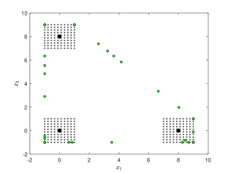
Example 6.1.
[2, Test Instance 5.2] Consider the function defined by
where the expression of , is given by
where , , and is an enumeration of the set with
Note that the set of the local weakly minimal points of is
For the evaluation of the performance of an algorithm, we have arbitrarily picked 100 initial points from the set . Then, we run all five conjugate gradient methods (proposed three—DY, PRP and HS—and two from [24]) for the same 100 initial points.
A summary of the performance of all the five methods is provided in Table 1. In this example, we observe that the performance of all the methods is almost identical.
The set of solutions generated by the HS method for the chosen 100 initial points is shown in Fig. 1 by green-colored bullets. In Fig. 1, three bigger size black-colored bullets represent the locations ; the three bunch of gray bullets collectively represent the set
. Notice that all the generated green-colored bullets are weakly minimal points of the set-valued function .
| Method | Iteration counts | Time | ||||
|---|---|---|---|---|---|---|
| min | mean | max | min | mean | max | |
| DY | 1 | 1.04 | 3 | 0.3457 | 1.6164 | 14.5765 |
| PRP | 1 | 1.03 | 2 | 0.3457 | 1.4872 | 8.7392 |
| HS | 1 | 1.03 | 2 | 0.3457 | 1.4238 | 10.7682 |
| FR | 1 | 1.04 | 3 | 0.3457 | 1.5256 | 10.6281 |
| CD | 1 | 1.04 | 3 | 0.3457 | 2.0030 | 22.2712 |
Example 6.2.
In this problem, we consider the function defined by
where the expression of , is given by
In this example, computer codes of all the five conjugate gradient methods are run for the same set of 100 initial points, which are arbitrarily chosen from the domain . A summary of the performance of the five methods is presented in Table 2. We note that for this example, Algorithm 1 with PRP rule performs better than the other four methods.
| Method | Iteration counts | Time | ||||
|---|---|---|---|---|---|---|
| min | mean | max | min | mean | max | |
| DY | 0 | 11.02 | 84 | 1.3270 | 50.4930 | 367.7961 |
| PRP | 0 | 5.52 | 40 | 1.3270 | 24.6789 | 157.8450 |
| HS | 0 | 6.78 | 91 | 1.3270 | 36.9255 | 331.9024 |
| FR | 0 | 11.98 | 195 | 1.3270 | 55.3178 | 1210.6040 |
| CD | 0 | 7.94 | 62 | 1.3270 | 82.8473 | 335.9404 |
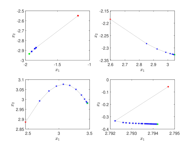
In Figure 2, we exhibit the movement of the sequence of iterates generated by Algorithm 1 with PRP rule corresponding to the following four initial points ():
| (54) |
In all the four subfigures in Fig. 2, the initial point of the sequence is depicted by red color, the terminal by green, and the intermediate ones by blue.
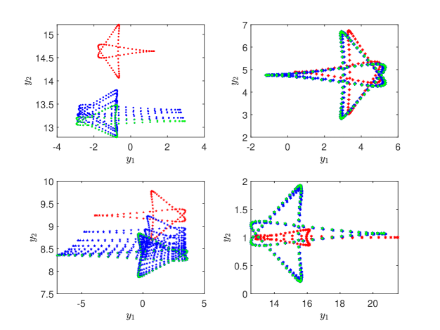
The movement of the sequence (in the image space) corresponding to the four different sequences plotted in Fig. 2 are depicted in the four different subfigures in Fig. 3. The top-left, top-right, bottom-left, and bottom-right subfigure in Fig. 3 are corresponding to the top-left, top-right, bottom-left, and bottom-right subfigure in Fig. 2, respectively.
The red-colored bullet point in the top-left subfigure of Fig. 2 is the initial point ; the bunch of red-colored bullets in the top-left subfigure of Fig. 3 is the set . The green-colored bullet in the top-left subfigure of Fig. 2 is the terminal point ( say) of the sequence ; the bunch of green-colored bullets in the top-left subfigure of Fig. 3 is the set . Similarly, the set corresponding to the intermediate points in are also depicted.
In the same fashion as the correspondence of the top-left subfigures of Fig. 2 and Fig. 3, the top-right, bottom-left and bottom-right subfigures in Fig. 3 are generated.
Example 6.3.
We consider the function defined as
where ,
and
Note that
Here, the function is derived from the well-known MOP7 test problem [13] for vector optimization.
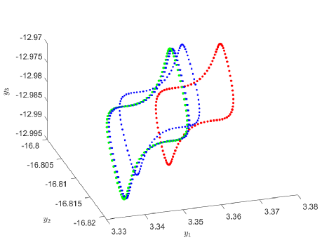
The computer codes of all five conjugate gradient methods were executed using the same set of 100 initial points, arbitrarily selected from the domain . A performance summary of these five methods is provided in Table 3. Notably, for this example, Algorithm 1 implementing HS rule outperformed the other four methods.
In Fig. 4, we exhibit the sequence of set-valued iterates corresponding to the sequence , which is generated by Algorithm 1 with HS rule for the initial point . The bunch of red-colored bullets, in Fig. 4, is the set , the blues ones are intermediate ’s, and the green bunch represents the terminal .
| Method | Iteration counts | Time | ||||
|---|---|---|---|---|---|---|
| min | mean | max | min | mean | max | |
| DY | 3 | 42.5938 | 142 | 64.7456 | 218.7738 | 1012.4873 |
| PRP | 5 | 23.0729 | 266 | 51.1373 | 157.0143 | 1747.0088 |
| HS | 3 | 17.5833 | 204 | 44.2141 | 138.9676 | 1270.7534 |
| FR | 4 | 36.3500 | 194 | 54.8662 | 164.8179 | 828.6454 |
| CD | 3 | 41.2641 | 430 | 67.6458 | 174.9024 | 1811.7712 |
In the next experiment, the set-valued mapping is taken from [2, Test Instance 5.1].
Example 6.4.
Consider , defined as
| (55) |
where for each is given by
In this example, we consider two different set optimization problems () with the same objective function but with different ordering cones and , where
| (56a) | ||||
| (56b) | ||||
For both problems, we run computer codes of all the five conjugate gradient methods for the same 100 initial points chosen arbitrarily from the interval . A summary of the performance of the five methods is given in Table 4 and Table 5 corresponding to cones and , respectively. As seen from Tables 4 and 5, although the performance of all five methods is almost identical, the HS rule slightly outperforms the other four methods.
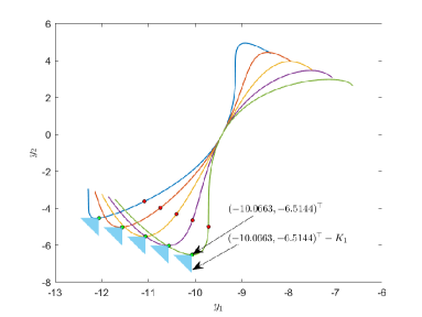
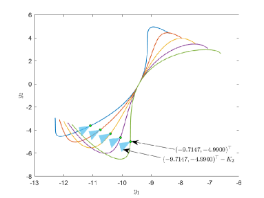
The sequence of sets corresponding to the generated sequence by Algorithm 1 with the HS rule and the initial point is depicted in Fig. 5. The five curves in both the subfigures of Fig. 5 are graphs of the functions , . The collection of the red-colored bullet points is the set , and the collection of green-colored bullet points is the value of at the terminal iterate.
The collection of the green bullet points on the right subfigure of Fig. 5 is the set , where . From this subfigure, we see that the green curve and the violet curve do not have a local portion in the sky-blue-shaded region. Thus, is a local weakly minimal point of the considered set optimization problem with the ordering cone . Hence, Algorithm 1 gets terminated at the initial point .
From the left subfigure of Fig. 5, we see that the bunch of red-colored bullet points is the set , which is not a local weakly minimal solution of the considered set optimization problem with the ordering cone since all the five graphs of the functions , have local portion inside the set . Thus, is not a local weakly minimal point of the considered set optimization problem with the ordering cone . Hence, for , Algorithm 1 does not get terminated at the initial point . In fact, for , Algorithm 1 with HS rule gets terminated in the next iterate at which the objective function value is the set of all green-colored bullet points in the left subfigure of Fig. 5.
| Method | Iteration counts | Time | ||||
|---|---|---|---|---|---|---|
| min | mean | max | min | mean | max | |
| DY | 0 | 1.01 | 4 | 0.2614 | 2.6601 | 13.1601 |
| PRP | 0 | 1.04 | 4 | 0.2614 | 2.8637 | 13.7649 |
| HS | 0 | 0.99 | 4 | 0.2614 | 2.5884 | 12.8843 |
| FR | 0 | 1.02 | 5 | 0.2614 | 2.8565 | 17.1513 |
| CD | 0 | 1.01 | 5 | 0.2614 | 2.7202 | 16.3896 |
| Method | Iteration counts | Time | ||||
|---|---|---|---|---|---|---|
| min | mean | max | min | mean | max | |
| DY | 0 | 0.04 | 1 | 0.2863 | 0.3188 | 5.0179 |
| PRP | 0 | 0.04 | 1 | 0.2863 | 0.3188 | 5.0179 |
| HS | 0 | 0.04 | 1 | 0.2863 | 0.3188 | 5.0179 |
| FR | 0 | 0.04 | 1 | 0.2863 | 0.3188 | 5.0179 |
| CD | 0 | 0.04 | 1 | 0.2863 | 0.3188 | 5.0179 |
Next, we consider an example where the image space of the objective function is , but the ordering cone is not the usual .
Example 6.5.
Similar to Example 6.4, consider two set-valued optimization problems with the identical objective function but with two different cones:
| (57a) | ||||
| (57b) | ||||
where
| (58) |
with
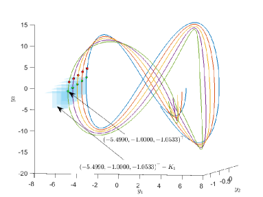
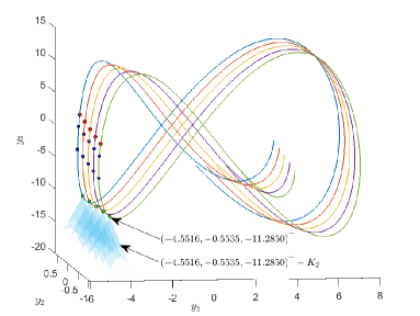
Note that the cone is finitely generated, but is not finitely generated.
For the problem with , we run the computer code of all the five conjugate gradient methods for the same 100 initial points that are arbitrarily picked from the interval . A summary of the performance of the five methods is presented in Table 6. Notice from Table 6 that although all the methods perform equivalently, the DY rule has just a slightly better performance than the other four methods.
For the problem with , we run the computer code of all the proposed three conjugate gradient methods for the same, arbitrarily picked, 100 initial points from . A summary of the performance is provided in Table 7. Notice from Table 7 that the DY rule has better performance than the other two methods. As the approaches described in [24] are not applicable for nonfinitely generated cones, for the problem with , we do not compare the proposed three conjugate gradient rules with the FR and CD methods in [24].
The sequence of sets corresponding to the sequence generated by Algorithm 1 with DY rule for the initial point are exhibited in Fig. 6. The left subfigure corresponds to , and the right corresponds to . The curves in both the subfigures are the graphs of the functions , . The bunch of red-colored bullet points is the set , and the green bunch is the value of the function at the terminal iterate. Blue-colored points are used to depict the value of at the intermediate iterates. Note that for the same initial point , the solutions generated by the same method are different for different ordering cones and .
| Method | Iteration counts | Time | ||||
|---|---|---|---|---|---|---|
| min | mean | max | min | mean | max | |
| DY | 0 | 0.64 | 5 | 0.1790 | 1.9988 | 14.9486 |
| PRP | 0 | 0.66 | 5 | 0.1790 | 2.1551 | 15.3702 |
| HS | 0 | 0.65 | 5 | 0.1790 | 2.0057 | 15.0421 |
| FR | 0 | 0.65 | 5 | 0.1790 | 2.0149 | 17.7405 |
| CD | 0 | 0.64 | 5 | 0.1790 | 2.0013 | 16.8554 |
| Method | Iteration counts | Time | ||||
|---|---|---|---|---|---|---|
| min | mean | max | min | mean | max | |
| DY | 0 | 0.15 | 3 | 0.1225 | 0.5538 | 1.7311 |
| PRP | 0 | 0.15 | 3 | 0.1225 | 0.5575 | 1.6302 |
| HS | 0 | 0.15 | 3 | 0.1225 | 0.5600 | 1.6680 |
7 Conclusion
In this work, nonlinear conjugate gradient methods have been proposed to identify local weakly minimal points of the set optimization problem () under the lower set less preordering relation. We have introduced the concept of -descent direction and a sufficient descent condition for set-valued functions with the help of an auxiliary real-valued function. With the help of this auxiliary function, we have introduced the standard and strong Wolfe line searches for set-valued functions. Following this, we have established a result (Theorem 3.1 and Remark 3.1) on the existence of a step size for which the standard Wolfe or strong Wolfe conditions are satisfied. Then, we reported (in Theorem 3.2) that for a given sequence of -descent directions of a set-valued function, any sequence of iterates defined by satisfies a Zoutendijk-like condition if the step size sequence satisfies the proposed standard Wolfe condition. Importantly, this step size existence result is derived without assuming that the ordering cone is finitely generated. Thereby, all the derived results in this study are applicable even for nonfinitely generated ordering cone .
Thereafter, we have proposed a general scheme (Algorithm 1) for nonlinear conjugate gradient methods for the set optimization problem. Then, we have reported (Proposition 4.1) some choices of -value so that the direction given in the general conjugate gradient Algorithm 1 is -descent and sufficient descent. Subsequently, without explicitly restricting the parameter , we have proved the global convergence (Theorem 4.1) of the proposed algorithm.
Next, we have proposed the DY, PRP, and HS rules to choose the value for set optimization problems. Then, in Theorem 5.1 and Theorem 5.2, we have established the convergence of the proposed Algorithm 1 with DY, PRP, and HS rules. Finally, we have conducted numerical experiments to demonstrate the performance of the proposed methods. A comparison of the proposed DY, PRP and HS methods with the existing FR and CD methods for set optimization is also provided.
In the future, one may try to address the following issues.
-
•
As mentioned in Remark 4.1, a regular restart condition is used in Step 4 to make as a -descent direction of at . In the future, we may work on a new line search technique so that no regular restart condition is required.
- •
-
•
Applying the proposed methods, future research may aim to find techniques to solve uncertain optimization problems with finite uncertainty.
-
•
No result on the rate of convergence of the proposed algorithm is derived in this study. Future studies can be done in this direction.
-
•
As the Gerstewitz scalarizing function requires a prespecified , which may not be easy to choose, analysis of the proposed results with respect to other scalarizing functions can be done in the future. Also, in this paper, we have used the lower set less ordering of sets to derive results. Future work can use other preordering relations of sets to see if the derived results hold.
Acknowledgement
Debdas Ghosh acknowledges the financial support of the research grants MATRICS (MTR/2021/000696) and Core Research Grant (CRG/2022/001347) by the Science and Engineering Research Board, India. Ravi Raushan thankfully acknowledges financial support from CSIR, India, through a research fellowship (File No. 09/1217(13822)/2022-EMR-I) to carry out this research work.
Data availability
There is no data associated with this paper.
References
- [1] Ben-Tal, A., Nemirovski, A.: Robust convex optimization. Math. Oper. Res. 23(4), 769–805 (1998)
- [2] Bouza, G., Quintana, E., Tammer, C.: A steepest descent method for set optimization problems with set-valued mappings of finite cardinality. J. Optim. Theory Appl. 190(3), 711–743 (2021)
- [3] Drummond, L.M.G., Svaiter, B.F.: A steepest descent method for vector optimization. J. Comput. Appl. Math. 175(2), 395–414 (2005)
- [4] Ehrgott, M., Ide, J., Schöbel, A.: Minmax robustness for multi-objective optimization problems. Eur. J. Oper. Res. 239(1), 17–31 (2014)
- [5] Eichfelder, G., Niebling, J., Rocktäschel, S.: An algorithmic approach to multiobjective optimization with decision uncertainty. J. Glob. Optim. 77(1), 3–25 (2020)
- [6] Eichfelder, G., Jahn, J.: Vector optimization problems and their solution concepts. In: Recent Developments in Vector Optimization. Vector Optim., pp. 1–27. Springer, Berlin (2012)
- [7] Gilbert, J.C., Nocedal, J.: Global convergence properties of conjugate gradient methods for optimization. SIAM J. Optim. 2(1), 21–42 (1992)
- [8] Gonçalves, M.L.N., Lima, F.S., Prudente, L.F.: A study of Liu-Storey conjugate gradient methods for vector optimization. Appl. Math. Comput. 425, 127099 (2022)
- [9] Gonçalves, M.L.N., Prudente, L.F.: On the extension of the Hager–Zhang conjugate gradient method for vector optimization. Comput. Optim. Appl. 76(3), 889–916 (2020)
- [10] Günther, C., Köbis, E., Popovici, N.: Computing minimal elements of finite families of sets w.r.t. preorder relations in set optimization. J. Appl. Numer. Optim. 1(2), 131–144 (2019)
- [11] Günther, C., Köbis, E., Popovici, N.: On strictly minimal elements w.r.t. preorder relations in set-valued optimization. Appl. Set-Valued Anal. Optim. 1(3), 205–219 (2019)
- [12] He, Q.R., Chen, C.R., Li, S.J.: Spectral conjugate gradient methods for vector optimization problems. Comput. Optim. Appl. 86(2), 457–489 (2023)
- [13] Huband, S., Hingston, P., Barone, L., While, L.: A review of multiobjective test problems and a scalable test problem toolkit. IEEE Trans. Evol. Comput. 10(5), 477–506 (2006)
- [14] Ide, J., Köbis, E.: Concepts of efficiency for uncertain multi-objective optimization problems based on set order relations. Math. Methods Oper. Res. 80(1), 99–127 (2014)
- [15] Ide, J., Köbis, E., Kuroiwa, D., Schöbel, A., Tammer, C.: The relationship between multi-objective robustness concepts and set-valued optimization. Fixed Point Theory and Appl. 2014, 1–20 (2014)
- [16] Jahn, J.: A derivative-free descent method in set optimization. Comput. Optim. Appl. 60(2), 393–411 (2015)
- [17] Jahn, J.: A derivative-free rooted tree method in nonconvex set optimization. Pure Appl. Funct. Anal. 3(4), 603–623 (2018)
- [18] Jahn, J., Ha, T.X.D.: New order relations in set optimization. J. Optim. Theory Appl. 148(2), 209–236 (2011)
- [19] Jiang, L., Cao, J., Xiong, L.: Generalized multiobjective robustness and relations to set-valued optimization. Appl. Math. Comput. 361, 599–608 (2019)
- [20] Karaman, E., Soyertem, M., Atasever, G.I., Tozkan, D., Küçük, M., Küçük, Y.: Partial order relations on family of sets and scalarizations for set optimization. Positivity 22(3), 783–802 (2018)
- [21] Khan, A.A., Tammer, C., Zalinescu, C.: Set-Valued Optimization. Springer, Heidelberg (2015)
- [22] Köbis, E., Köbis, M.A.: Treatment of set order relations by means of a nonlinear scalarization functional: a full characterization. Optimization 65(10), 1805–1827 (2016)
- [23] Köbis, E., Le, T.T: Numerical procedures for obtaining strong, strict and ideal minimal solutions of set optimization problems. Appl. Anal. Optim. 2(3), 423–440 (2018)
- [24] Kumar, K., Ghosh, D., Yao, J.-C., Zhao, X.: Nonlinear conjugate gradient methods for unconstrained set optimization problems whose objective functions have finite cardinality. Optimization. (2024) https://doi.org/10.1080/02331934.2024.2390116
- [25] Kuroiwa, D.: The natural criteria in set-valued optimization. Sūrikaisekikenkyūjo kōkyūroku 1031, 85–90 (1998)
- [26] Köbis, E., Tammer, C., Kuroiwa, D.: Generalized set order relations and their numerical treatment. Appl. Anal. Optim. 1(1), 45–65 (2017)
- [27] Kuroiwa, D.: On set-valued optimization. Nonlinear Anal. Theory Methods Appl. 47(2), 1395–1400 (2001)
- [28] Kuroiwa, D.: Some criteria in set-valued optimization. Sūrikaisekikenkyūjo kōkyūroku 985, 171–176 (1997)
- [29] Pérez, L.L.R., Prudente, L.F.: A Wolfe line search algorithm for vector optimization. ACM Trans. Math. Softw. 45(4), 1–23 (2019)
- [30] Pérez, L.L.R., Prudente, L.F.: Nonlinear conjugate gradient methods for vector optimization. SIAM J. Optim. 28(3), 2690–2720 (2018)
- [31] Mutapcic, A., Boyd, S.: Cutting-set methods for robust convex optimization with pessimizing oracles. Optim. Methods Softw. 24(3), 381–406 (2009)
- [32] Nishnianidze, Z.G.: Fixed points of monotone multivalued operators. Soobshch. Akad. Nauk Gruzin. SSR 114(3), 489–491 (1984)
- [33] Schmidt, M., Schöbel, A., Thom, L.: Min-ordering and max-ordering scalarization methods for multi-objective robust optimization. Eur. J. Oper. Res. 275(2), 446–459 (2019)
- [34] Yahaya, J., Kumam, P.: Efficient hybrid conjugate gradient techniques for vector optimization. Results Control Optim. 14, 100348 (2024)
- [35] Young, R.C.: The algebra of many-valued quantities. Math. Ann. 104(1), 260–290 (1931)