Motivated by the observation of the resonance in the system by the BESIII collaboration, we studied the molecular states of hexaquarks and with baryon-antibaryon structures within the framework of the QCD sum rules. Non-perturbative contributions up to dimension 13 were considered in our analysis. The results indicate the existence of six possible molecular states and , with quantum numbers . Consequently, the current sum rule results do not support the interpretation of as a or molecular state. On the other hand, we find that the masses of the proposed and structures with are in the vicinity of observed , which implies that the nature of this state needs more invistigations. Moreover, the possible decay modes of the concerned hexaquark states are analyzed.
I Introduction
In the 1960s, to explain new particles discovered in large colliders, Gell-Mann et al. proposed the quark model (QM) [1, 2], marking the beginning of human exploration of strong interactions. By 1973, with the establishment of quantum chromodynamics (QCD), the theory describing strong interactions was essentially complete. QCD calculations are fundamentally performed at the level of quarks and gluons. However, no free quarks or gluons have been observed experimentally so far; only hadrons, which are composed of quarks and gluons, can be detected. Therefore, studying the properties of hadrons can help us understand strong interactions and enrich our knowledge of the microscopic world.
Traditional hadronic states include mesons and baryons , while other configurations of hadrons, such as hybrid states, glueballs and multi-quark states more than three quarks, are also allowed by the QM. In 2003, the Belle Collaboration discovered a new resonance state [3], considered as a bound-state particle with a tetraquark structure [4, 5, 6, 7, 8, 9]. Over the past two decades, with the development of experimental technology, numerous exotic hadron states have been discovered [10, 11, 12, 13, 14, 15, 16]. Currently, experimentally observed exotic hadronic states include tetraquark states and pentaquark states [10, 17, 18]. Research on the properties of exotic hadronic states has garnered widespread attention worldwide and has become an important area in particle physics.
Theoretically, there are various methods for studying exotic states, including quark models [1, 2], the MIT bag model [19], lattice QCD [20], chiral effective theory [21], AdS/QCD [22], and QCD sum rules (QCDSR) [23, 24], etc. Among these, the QCDSR method proposed by Shifman, Vainshtein, and Zakharov (SVZ) is based on the first principles of QCD and effectively incorporates the non-perturbative contributions of QCD. QCDSR is a well-established and effective approach for investigating hadron properties, providing analytical expressions for hadron masses [23, 24, 25, 26, 27], form factors [28, 29, 30, 31, 32, 33, 34, 35], decay constants [36, 37, 38, 39, 40], and other observables [41]. For the first discovered exotic state , QCDSR has successfully provided explanations for its structure [7, 8, 9].
Since both tetraquark and pentaquark states have been observed, the study of hexaquark states should be prioritized. The first studied hexaquark state is the dibaryon, a bound state composed of two baryons. Although many theoretical predictions have been made [42, 43, 44, 45, 46, 47, 48, 49], it has yet to be observed experimentally [50]. Another typical hexaquark structure is the molecular state of baryon-antibaryon, where baryonium is a typical structure. The heavy baryonium has been used to explain the structure of [51, 52, 53]. Subsequently, a series of theoretically predicted light baryonium states have been proposed in QCDSR [54, 55], which can also successfully explain the structures of [56] and [57] observed in experiments. Furthermore, QCDSR has also provided predictions for the mass spectra of other baryonium states [58, 59, 60].
Hexaquarks can form not only as baryonium states composed of a baryon and its corresponding antibaryon but also as bound states made up of different baryons. Experimentally, several structures have been observed in the final state of , including [61] and the recently discovered [62], both of which lie close to the threshold of . Among them, the quantum number of has been determined to be . Theoretically, and could be interpreted as a baryon-antibaryon molecular state of the structure . Furthermore, other structures with near thresholds and the same quantum numbers should also be considered, where the closest candidate being the molecular state [63]. Therefore, studying the mass spectrum of the molecular state of the wave and could provide more insight into the nature of and . The molecular states and belong to the flavor SU(3) nonet [64], and studies based on the quark models have already provided preliminary calculations of their mass spectra [65, 63].
In this work, we will determine the mass spectra of the ground molecular states and within the framework of QCDSR. The results will be compared with experiment, and potential decay modes will be analyzed. The structure of this paper is organized as follows: in Sect.II, we briefly introduce the theoretical framework of QCDSR and present the fundamental formulas used in our calculations. In Sect.III, we provide numerical analyses and results. Sect.IV discusses the possible decay modes of and . Finally, in Sect.V, we compare our results with experimental observations and summarize our findings.
II Formalism
II.1 Choices of the Currents
In the framework of QCDSR, to calculate the mass spectrum of and , it is essential to first select appropriate hadronic interpolating currents. There are two independent interpolating currents for the baryon octet[66], and the other interpolating current structures can be obtained by linear combinations of them through Fierz transformations [67]. In our calculation, the mass of quarks are rather smaller than the -quark, so we take the limit , which simplifies the structure of the interpolating currents. The two simplified interpolating currents we have chosen are [68, 69]
(1)
(2)
where for , the indices take the following values: for , for , and for . are the color indices. denotes an arbitrary light baryon.
For the baryon-antibaryon type hexaquark molecular states , the quantum numbers of the ground states will take , and the corresponding interpolating current structures are given by
(3)
(4)
(5)
(6)
where the two baryonic interpolating currents and for each molecular state must be chosen uniformly from either Eq.(1) or (2), respectively. Thus, for each baryonic interpolating current, there exist four possible molecular state structures of hexaquark, corresponding to four different quantum numbers .
II.2 2-point Correlation Functions
After selecting the interpolating currents Eqs.(3)-(6), we can evaluate the two-point correlation functions of the interpolating currents
(7)
(8)
where are the interpolating currents corresponding to the molecular states with , respectively, and represents the physical QCD vacuum state. The tensor-type correlation function can not fully represent the molecular state. It can be written as the sum of two parts
(9)
where the subscripts and correspond to particles with spin and , respectively. By projecting, we obtain
(10)
which is the two-point correlation function for the molecular state current.
II.2.1 OPE Side
We can analytically evaluate the correlation functions given in Eqs.(7)-(8). For the Type-1 baryon current Eq.(1), the correlation functions in coordinate space are denoted as
(11)
(12)
(13)
(14)
where are color indices, and correspond to the quantum numbers and , respectively. Similarly, correspond to the quantum numbers and , respectively. For the Type-2 baryon current Eq.(2), the correlation functions are similarly given by
(15)
(16)
(17)
(18)
The propagator in the above correlation functions represents the full QCD propagator, which incorporates both perturbative and non-perturbative contributions at all orders of vacuum condensates. The full propagator for a light quark can be expressed as
(19)
More details on the full propagator can refer to Refs.[70, 71]. The typical Feymann diagrams of the correlation functions are shown in Fig.1, which also includes the contributions of the non-perturbative vacuum condensates.
Figure 1: The typical Feynman diagrams for the two-point correlation functions are shown, where the thick lines represent light quarks, the spiral lines denote gluons, and the solid dots indicate the condensates. The diagrams include contributions from the perturbative term, quark condensates, gluon condensates, and mixed condensates.
Through the Källén-Lehmann spectral representation
(20)
we can correspond the correlation functions given in Eqs.(11)-(18) to the spectral density and derive the spectral density in the form of the operator product expansion (OPE). The spectral density, including vacuum condensates up to dimension 13, can generally be expressed as
(21)
Subsequently, through the dispersion relation, the spectral density on the OPE side can be used to express the correlation function as
(22)
where denotes the corresponding ground hadronic state and denotes its quantum number; represents the kinematic threshold, typically corresponding to the sum of the masses of all quarks involved in the hadronic interpolating current [27, 26, 54], i.e. for and molecular states. The analytical results of are shown in the appendices.
II.2.2 Phenomenological Side
In the phenomenological side, the contributions from the ground state and excited states to the spectral density can be separated as
(23)
where and represent the decay constant and mass of the ground state, respectively; represents the threshold of the continuum spectrum, above which the spectral density should include contributions from higher excited states and the continuum spectrum. Consequently, the phenomenological correlation function can be expressed through the dispersion relation as
(24)
II.3 Hadronic Mass
According to the principle of quark-hadron duality , the correlation functions from both the OPE and the phenomenological sides should be consistent. Above the continuum threshold , the spectral density satisfies . Based on this principle, we combine the two sides of the correlation function Eqs.(22), (24) and apply the Borel transformation to both sides, which suppresses the contributions from higher excited states and the continuum, yielding
(25)
From the above equation, the mass of the ground-state hadron can be determined as
(26)
where
(27)
Here, represents the part of the correlation function that has no imaginary part but provides non-trivial contributions after the Borel transformation, which are proportional to the masses of quarks. Since we have taken the limit , this contribution vanishes and does not appear in our calculations.
III Numerical Analysis
In the numerical calculations of QCDSR, we adopt the following input parameters [41, 72, 54], where represents the quarks:
(28)
In the process of establishing QCDSR, we also introduce two additional parameters, namely the continuum threshold parameter and the Borel parameter . Theoretically, the mass should not depend on these two parameters. Therefore, it is necessary to identify a range of and in which the variation of remains relatively stable. This range of parameters is the so-called Borel window. To determine an appropriate Borel window, we need to introduce two criteria. First, since we are calculating the mass of the ground-state hadron, the pole contribution should dominate. According to Eq.(LABEL:moment), the contribution to the spectral density from is significantly suppressed [73, 74, 75]. Therefore, the fraction of pole contribution can be defined as
(29)
For hexaquark states, we assume that this value should be no less than [58, 54]. Secondly, the OPE should converge, which means that the contribution from the highest-dimensional condensate should be as small as possible. In this work, we calculate the contributions to the spectral density up to the dimension 13 condensates. The ratio of the dimension 13 condensate contribution is defined as
(30)
where
(31)
To determine the range of , we adopt the method proposed in Refs.[27, 26, 54, 76, 77]. First, since represents the threshold for the onset of the continuum spectrum, it should be slightly larger than the hadron mass , that is, , where is typically taken as [41, 54, 78]. Next, within this interval of , we search for the range of where the mass remains nearly stable. Since the contribution to the spectral density of is significantly suppressed, the region is pole dominated. Therefore, should characterize the energy scale of the hadron . The range of and that satisfies the above requirements is the Borel window, which corresponds to the physical state of the hadron under our investigation. In practice, we allow to vary within a range of . A stable physical state is identified when the variation of within the Borel window exceeds , ensuring the stability of the results.
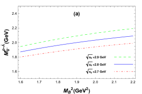
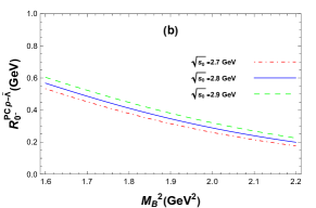
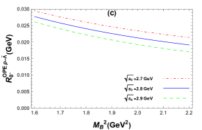
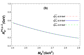
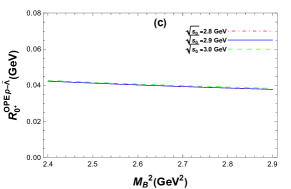
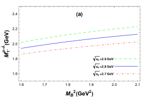
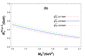
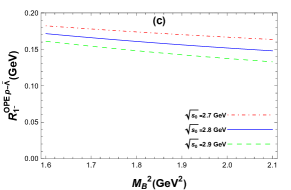
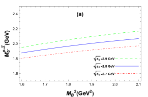
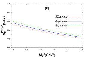
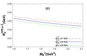
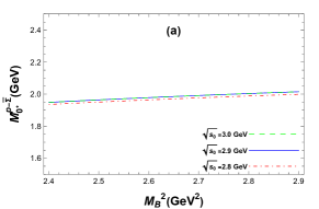
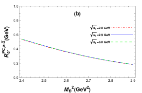
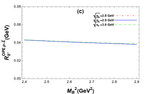
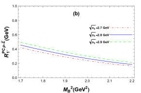
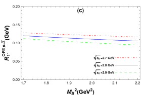
Based on the above discussion, we performed numerical calculations for the mass spectra of the ground states of the and molecular states. For the states, we identified the Borel windows that satisfy the requirements for the states of the Type-1 current and the states of the Type-2 current. For the other states, no suitable Borel window could be identified regardless of the choice of and . Therefore, we conclude that the corresponding current does not couple to such states, which is consistent with our previous work on the light bayronium [54]. The choices of Borel windows and the mass of states are shown in Table.1. For the state, the dependence relationships between and is shown in Fig.2(a), and the ratios and are shown as functions of in Fig.2(b) and Fig.2(c) with different values of , respectively. The same figures for and states are shown in Fig.3 and Fig.4 , respectively.
Current
Type-1
Type-2
Table 1: The continuum thresholds, Borel parameters, and predicted masses of molecular states
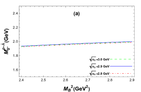
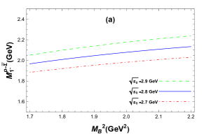
For the state, we obtained similar results. We identified the Borel windows that satisfy the requirements for the states of the Type-1 current and the states of the Type-2 current. For the other states, no suitable Borel window could be identified regardless of the choice of and , either. Choices of Borel windows and the mass of them are shown in Table.2. The figures for the above 3 states are shown in Figs.5, 6, 7, respectively.
Figure 2: The figures for the state: (a) The mass as a function of for different values of . (b) The ratio as a function of for different values of . (c) The ratio as a function of for different values of .
Figure 3: The same caption as Fig.2 but for the state.
Figure 4: The same caption as Fig.2 but for the state.
Figure 5: The same caption as Fig.2 but for the state.
Figure 6: The same caption as Fig.2 but for the state.
Figure 7: The same caption as Fig.2 but for the state.
Current
Type-1
Type-2
Table 2: The same table as Table.1 but for atates.
From Tables.1, 2, it can be observed that the mass results of the hexaquark states exhibit uncertainties. These uncertainties arise from the input quark masses, the vacuum condensates, and the choices of and . We also compared our results with those calculated through constituent quark models without annihilation interactions [63], including the chiral quark model (ChQM) and the quark delocalization color-screening model (QDCSM) in Table.3. In this comparison, we adopted the mass data of , and from the Particle Data Group (PDG) [79]. It can be seen that the results for obtained from both models are less than the corresponding dibaryon threshold. However, for , the results from the chiral quark model exceed the corresponding dibaryon threshold, which is rather larger than the central values of our results.
This work
QDCSM
ChQM
2.00
2.045
2.045
1.96
2.05
2.048
2.047
1.99
2.132
2.165
1.98
2.06
2.152
2.189
Table 3: The comparison between hexaquark state masses obtained in this work and the results from the constituent quark model.
IV Decay Modes Analyses
To search for these hexaquark states experimentally, the simplest and most direct approach is to reconstruct them from their decay products. In this section, we provide the possible decay modes of the six and molecular states studied earlier, with the hope that they can be observed on the running experiments like the BESIII, BELLEII, and LHCb. Since the masses of these molecular states are all below their corresponding diquark thresholds, their direct decays into or are forbidden. The remaining possible decay modes are listed in Table.4.
Modes of ()
Table 4: Typical decay modes of the and molecular states for each quantum number.
V Discussion and Conclusions
We investigated the ground state mass spectra of the hexaquark molecular configurations and with the four quantum numbers: in the QCDSR framework. Two independent octet baryonic currents were chosen to establish the QCDSR. The results indicate that only the hexaquark states and with exist, with masses below their corresponding diquark thresholds. Since the quantum number of have already been confirmed as , and our results indicate the absence of and with , we exclude the possibility of of being this structure. On the other hand, the mass of lies close to the and molecular states. Based on these results, we also analyzed the possible decay modes of these six hexaquark states, leaving to experimental confirmation.
Acknowledgements.
We appreciate the enlightening discussion with Bing-Dong Wan and Liang Tang. This work was supported in part by the National Key Research and Development Program of China under Contracts No. 2020YFA0406400, by the National Natural Science Foundation of China(NSFC) under the Grants 12475087 and 12235008.
Gelhausen et al. [2013]P. Gelhausen, A. Khodjamirian, A. A. Pivovarov, and D. Rosenthal, Phys. Rev. D 88, 014015 (2013), [Erratum: Phys.Rev.D 89, 099901 (2014), Erratum: Phys.Rev.D 91, 099901
(2015)], arXiv:1305.5432
[hep-ph] .
In the appendix, the analytical results for the spectral densities are presented, corresponding to 16 different configurations, i.e., four quantum numbers for each of the two hexaquark states; and states with two different baryonic currents. In calculating the spectral densities, the FeynCalc package [80, 81, 82] was utilized to trace out the -matrices.
We expand the spectral densities as
(32)
where denotes for the dimension of the vacuum condensates.
Appendix A The Spectral Densities of Hexaquark States
A.1 Hexaquark States
A.1.1 Type-1 Current
(33)
(34)
(35)
(36)
(37)
(38)
(39)
(40)
(41)
(42)
(43)
(44)
A.1.2 Type-2 Current
(45)
(46)
(47)
(48)
(49)
(50)
(51)
(52)
(53)
(54)
(55)
(56)
A.2 Hexaquark States
A.2.1 Type-1 Current
(57)
(58)
(59)
(60)
(61)
(62)
(63)
(64)
(65)
(66)
(67)
(68)
A.2.2 Type-2 Current
(69)
(70)
(71)
(72)
(73)
(74)
(75)
(76)
(77)
(78)
(79)
(80)
A.3 Hexaquark States
A.3.1 Type-1 Current
(81)
(82)
(83)
(84)
(85)
(86)
(87)
(88)
(89)
(90)
(91)
(92)
A.3.2 Type-2 Current
(93)
(94)
(95)
(96)
(97)
(98)
(99)
(100)
(101)
(102)
(103)
(104)
A.4 Hexaquark States
A.4.1 Type-1 Current
(105)
(106)
(107)
(108)
(109)
(110)
(111)
(112)
(113)
(114)
(115)
(116)
A.4.2 Type-2 Current
(117)
(118)
(119)
(120)
(121)
(122)
(123)
(124)
(125)
(126)
(127)
(128)
Appendix B The Spectral Densities of Hexaquark States