Optimal Control for Open Quantum System in Circuit Quantum Electrodynamics
Abstract
We propose a quantum optimal control framework based on the Pontryagin Maximum Principle to design energy- and time-efficient pulses for open quantum systems. By formulating the Langevin equation of a dissipative LC circuit as a linear control problem, we derive optimized pulses with exponential scaling in energy cost, outperforming conventional shortcut-to-adiabaticity methods such as counter-diabatic driving. When applied to a resonator dispersively coupled to a qubit, these optimized pulses achieve an excellent signal-to-noise ratio comparable to longitudinal coupling schemes across varying critical photon numbers. Our results provide a significant step toward efficient control in dissipative open systems and improved qubit readout in circuit quantum electrodynamics.
Introduction.– Controlling quantum systems is fundamental for advancing quantum technologies, with quantum optimal control serving as a cornerstone. By modulating system parameters or applying external pulses, it enables precise manipulation of quantum dynamics, enhancing the performance of tasks like state preparation, gate operations, and qubit readout, all while adhering to platform-specific constraints [1, 2, 3, 4, 5]. One particularly powerful subset of quantum control techniques involves shortcuts to adiabaticity (STA) [6]. However, extending such techniques to dissipative or open quantum systems presents unique challenges due to the interaction between the system and its environment, which induces inevitable decoherence and dissipation effects [7, 8]. These considerations are crucial for realistic quantum technologies, as practical devices often operate in environments. Motivated by these challenges, STA methods have been adapted for open systems to mitigate dissipation and engineer quantum states under non-unitary dynamics. For example, inverse engineering and counter-diabatic (CD) driving (also known as transitionless quantum driving) have been successfully extended to open systems, facilitating efficient control over dissipative quantum dynamics [9, 10, 11, 12, 13, 14, 15, 16].
Among the diverse techniques for quantum control, the Pontryagin Maximum Principle (PMP) offers a rigorous mathematical framework for determining optimal solutions in both classical and quantum systems. PMP has been applied to a wide range of quantum tasks, including state preparation [17, 18], physical chemistry [19, 20], nuclear magnetic resonance [21, 22], quantum metrology [23] and quantum information processing [24]. By identifying the optimal trajectory that minimizes a specified cost function under the constraints, PMP enables the design of precise and efficient quantum control protocols for both closed and open systems [25, 26]. Furthermore, PMP’s capability to provide analytical solutions for shortcuts to isothermality facilitates rapid and energy-efficient thermodynamic processes [27].
In this Letter, we present optimized pulses for a driven-dissipative LC circuit, with a focus on circuit quantum electrodynamics (cQED) where superconducting qubits couple to microwave resonators [28, 29]. In cQED, the dissipation resulting from system-environment coupling offers an ideal platform for studying optimal control in open systems [15]. The optimal control strategies developed here are crucial not only for enhancing the fidelity of quantum state manipulation but also for improving dissipative qubit readout in cQED and, more broadly, in other similar systems involving qubit-cavity coupling [30, 31, 32, 33].
Here, we interpret the system’s Langevin equation (LE) as a linear control problem, which allows us to engineer quantum states with minimal time and low energy consumption. By applying the PMP [34, 35], we solve the control problem in the initial stage to obtain analytical pulses capable of transforming the quantum states for a single resonator. A key preliminary result can be stated as follows: these specific coherent states are characterized by fixed cavity displacements that minimize energy cost and optimize the time required for a given maximum driving amplitude, in comparison to the adiabatic sinusoidal pulse and its CD assistance [15]. In the second stage, these optimized pulses are used in non-demolition qubit readout across three different regimes: low, intermediate, and high critical photon numbers. Our findings indicate that for large critical photon numbers, the signal-to-noise ratio (SNR) is comparable to that of readout schemes based on longitudinal coupling [36, 37].
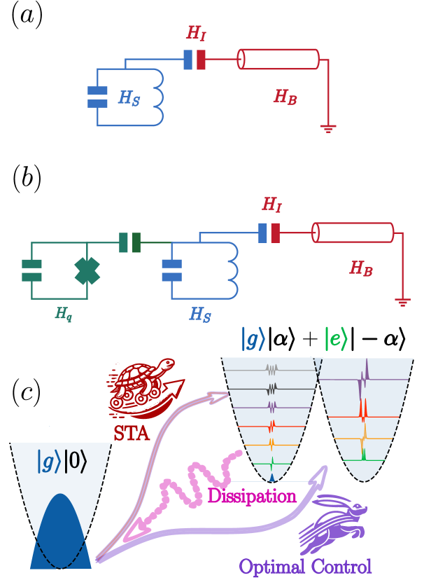
Single-resonator in open system.– The circuit in Fig. 1(a) consists of an LC oscillator, capacitively coupled to a transmission line resonator, representing the electromagnetic environment. The total Hamiltonian of the open system is given by (hereafter ), where the system Hamiltonian is with being the resonator frequency. The bath Hamiltonian is , representing a continuum of harmonic oscillators at frequencies . The interaction Hamiltonian is , describing the coupling between the resonator and the bath, where is the coupling strength. To derive the system dynamics, we trace out the reservoir degrees of freedom, arriving to the LE in the rotating frame [38, 39], , where is the system decay rate, and is the input field. By using time-dependent coherent state and relating the coherent driving field to the input field as , the LE becomes [40]
| (1) |
where the explicit time dependence of is omitted for simplicity. This equation also governs the dynamics of a coherent state in a driven harmonic oscillator in presence of dissipation [34], as described by the master equation [40] with . In the following, we outline the method for optimizing to drive the system from an initial state at to a desired target state at , while minimizing both the energy cost of the driving field and the required time.
Minimization of pulse energy and time.– Consider the control problem of linear system described by [34], where is the system state and is the control vector. Assuming the matrix is time-independent, the formal solution is , with the initial state . To minimize the functional , we incorporate the system’s dynamics into the optimization problem through the PMP. Regarding energy optimization, the cost function is . This leads to the Pontryagin Hamiltonian , where p is the adjoint variable, governed by . For energy minimization, we require , leading to and . Solving these equations for a time-independent , we find that the state vector can be written as
| (2) |
and the adjoint variable is . The constant vector is determined by the boundary condition, . Finally, the optimal control is obtained as [40]
| (3) |
Specifically, for the system with coherent state and driving field , substituting these into the control problem (1) yields the following system of equations:
| (4) |
By direct comparison, the state vector is , and the control vector is , with the corresponding matrices and . Using these, the optimal solution (3) becomes
| (5) |
which results in the optimal energy cost
| (6) |
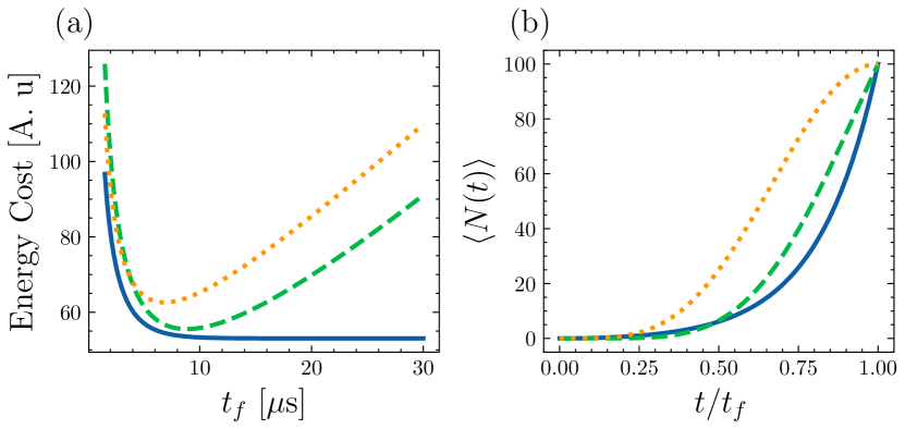
To assess the reduction in energy cost, we compare the optimized pulses with a typical Hahn (sinusoidal) pulse, defined as . The constant amplitude increases with , to satisfy the adiabatic criteria, ensuring that remains , with the fixed phase [40]. As illustrated in Fig. 2 (a), for small duration ( µs), both energy costs increase exponentially as the final time decreases, when the state evolves from to . However, in the adiabatic limit, µs, saturates to , whereas remains constant, . In Fig. 2 (b), both pulses achieve the same final photon number . However, the optimized pulse keeps the intermediate photon number lower throughout the process, highlighting its advantage in systems with pronounced anharmonicity and ionization [33].
The next step is to find the time-optimal driving field under a constraint, . To this end, we parameterize the real and imaginary components of the pulse as and , where is the phase to be optimized according to the PMP [41, 42]. To minimize the cost function , we define the Pontryagin Hamiltonian as , where (with ) are given by Eq. (4) and the constant represents an energy offset. The adjoint variable evolves according to the state equation , with and . The solution is given by . The energy conservation demands that ( is a constant), which leads to the initial conditions and . According to PMP, optimizing requires , which yields the condition , or equivalently, . Solving the LE in Eq. (1) using , we get
| (7) |
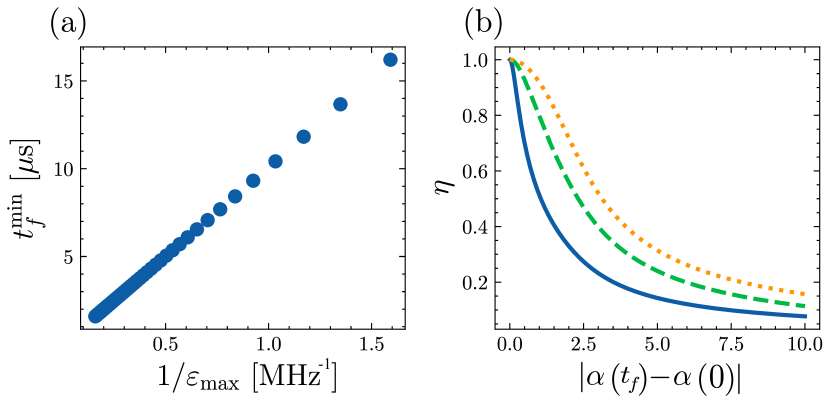
The optimal time is determined by minimizing . The phase is then adjusted to match the phase of with that of the target state . By satisfying these conditions, the system reaches the target state, e.g., , in the shortest possible time. Fig. 3(a) shows the minimal time as a function of , indicating an exponential decrease with increasing driving amplitude, e.g. µs when MHz.
To further compare the energy- and time-optimized pulses, the CD driving is given by [15]
| (8) |
where the adiabatic reference can be the Hahn pulse with a fixed [40]. Physically, this CD protocol can be implemented by driving the orthogonal quadrature resonator. In other words, for voltage-controlled pulses, the CD terms should be a current-controlled one, and vice versa. The inclusion of additional term guarantees to reach the equilibrium state without introducing the excited photons. Fig. 2(a) shows that, while the CD pulse is more energy-efficient than the Hahn pulse, it is still less efficient than the energy-optimal pulse. In the adiabatic limit, the CD pulse exhibits the same slope for the energy cost as the Hahn pulse, but with a constant residual energy.
To quantify the quantum speed limits [43], we invoke the Mandelstam-Tamm bound [44]: , where the geodesic distance between the initial and final states is determined by the Fubini-Study metric, and the standard deviation of the energy, , quantifies the energy uncertainty during the evolution. For our control problem involving coherent states, the effective Hamiltonian is given by , and the quantum efficiency is expressed as [15]:
| (9) |
with the energy uncertainty being . As illustrated in Fig. 3(b), the CD driving achieves the theoretical upper bound of efficiency, as the energy uncertainty precisely matches the additional term . In contrast, our optimal controls approach, but do not fully reach this bound, due to the constraint imposed on , rather than .
Qubit-resonator interaction.– We now extend the control framework to a system consisting of an LC resonator dispersively coupled to a qubit, as depicted in Fig. 1(b). In the dispersive approximation, the Jaynes-Cumming Hamiltonian is given by [45]
| (10) |
where is the qubit frequency, and is the effective Stark-shift, moreover, is the Pauli- operator. This Hamiltonian represents the conditional shift on the resonator frequency due to the qubit and vice versa, which can be used for qubit readout when the system is driven by an external field in LE [46]. For better readout contrast, larger driving amplitudes are needed to separate the qubit states more effectively on the resonator’s IQ plane. However, such amplitudes cannot exceed the fundamental limits imposed by the dispersive approximation that sets an upper bound on the photon number [47]. Moreover, the drive must be chosen carefully to avoid ionizing the artificial atom [48]. From the perspective of optimal control, it is essential to design the driving field that maximize both readout contrast and energy efficiency while ensuring the dispersive approximation holds and the artificial atom is not ionized.
We focus on system parameters resulting in three different critical photon numbers , which define the final boundary conditions for , i.e., . To maintain the validity of the dispersive approximation, we set the qubit-cavity detuning to GHz. Moreover, to engineer optimized readout pulses for the qubit-cavity system, we note that the Hamiltonian (10) shares the same LE (1), with the substitution , where is state-dependent Stark-shift [46, 30]. Consequently, we can obtain the optimal control for energy minimization using Eq. (5), which gives:
| (11) |
Similarly, we estimate the minimal control time under the constraint of maximal driving amplitude that ramps the resonator with photon numbers near using Eq. (7)
| (12) |
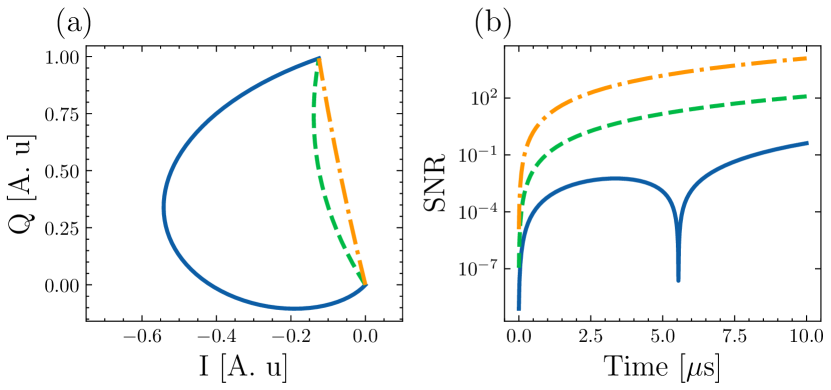
The primary difference from the single-resonator case is that the field displacement now depends on the qubit state. A larger separation between the qubit states leads to better readout outcome. Fig. 4(a) shows the normalized IQ plane of the resonator, corresponding to the real and imaginary parts of , when we initialize the qubit in the ground state , with a readout time of µs. Since the time is fixed, we apply the optimal protocol (11) for energy minimization in the subsequent calculations with corresponding to the solution for . The result for is equivalent as it only changes the direction in which the state displaces in the resonator phase space. The optimal pulse for smaller shows an exotic trajectory on the resonator IQ plane. This deviation arises due to the large coupling strength GHz, which is considerably higher than typical cQED implementations [28]. As a result, nonlinearities, such as Kerr effect, dominate the dynamics [49, 50] displacing the resonator state. The competition between these displacements modifies substantially the expected IQ trajectory. However, as the coupling strength decreases, the Kerr nonlinearities are suppressed, and the linear ramping becomes the dominant effect, as illustrated by the orange dot-dashed line in Fig. 4(a).
Another way to evaluate the performance of optimal pulses is by assessing the quality of the readout process using SNR. The SNR is defined as the ratio between the homodyne signal and its fluctuations. Specifically, the homodyne signal is given by , where the average homodyne signal for the state is defined as , with being the output field, determined by the input-output relation . Thus, the SNR is given by
| (13) |
where the fluctuations from the noise homodyne operator is . We illustrate the SNR behavior for three different critical photon numbers in Fig. 4(b), with . Similar to the IQ trajectory, the case exhibits exotic behavior. This case has the lowest SNR, as it is challenging to drive the resonator close to its critical value without significant pullback from the Kerr correction. As a result, the contrast between the states is not optimal, and noise dominates the signal. Additionally, the SNR evolution displays two minima, which stem from the exotic trajectory in the IQ plane: as the resonator states pass through origin multiple times, coherence is lost, causing the noise accumulation and a consequent SNR reduction. More details on time-optimal protocol (12) and CD driving are available in Ref. [40]. We demonstrate that energy-optimal control achieves higher SNR faster as compared to other schemes, and SNR under time-optimal driving reaches its maximum when , where .
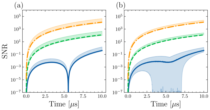
For larger , our optimized pulse exhibits a behavior comparable to cQED readout based on longitudinal coupling, as discussed in recent works [36, 37]. In these cases, the SNR is higher on a timescale shorter than the decay rate of the resonator. Moreover, the maximal peak of SNR increases monotonically with the critical photon number. This trend can be attributed to the fact that, as the photon number increases, the displacement in the resonator also becomes larger, thereby enhancing the contrast and facilitating better discrimination between qubit states. Additionally, it is possible to further improve SNR for these optimal pulses by initializing the resonator in a squeezed state [36].
To further evaluate the robustness of the optimized pulses, we analyze the SNR under 20 frequency errors [29] in both resonator and qubit subsystems across 1000 samples, as depicted in Fig. 5. For the resonator, frequency variations introduce oscillatory contribution in Eq. (1), affecting the pointer state’s trajectory yielding smaller SNR, whereas the mismatches on the qubit frequency modifies the dispersive approximation and consequently the critical photon number . The performance under typical parameter fluctuations shows that the energy-optimal pulses are more sensitive to errors at small , as these mismatches significantly alters , increasing the likelihood that the pulse drives the system beyond the dispersive approximation. In contrast, for larger critical photon numbers, the pulses demonstrate the robustness against parameter variations.
Conclusion.– In summary, we applied PMP to design time- and energy-optimised pulses for state transformation and non-demolition qubit readout in open quantum systems within cQED. Using the LE, we derived analytical pulses that respect various constraints. These optimized pulses efficiently engineer the displaced light states with fixed cavity displacement and photon number, exhibiting exponential scaling of energy cost with the operation time. The time-optimized pulse achieves microsecond-scale duration at MHz driving amplitudes. For high-fidelity readout, in dispersively coupled resonator-qubit systems, our optimal pulses achieve nearly unit SNR within a timescale shorter than the resonator’s decay rate for large critical photon numbers.
Our work paves the way for similar pulse optimization in other platforms, such as quantum dots [51, 52, 53]. Future research could explore numerical optimization [54] or machine learning [55, 56, 57, 58] to improve robustness against errors and noise, addressing more complex optimization problems involving decoherence and anharmonicity. Yet, this study not only explores fundamental speed limits [59, 60] in quantum open systems, but also supports practical applications in dissipative qubit readout within cQED.
Acknowledgement.– We are grateful to Sigmund Kohler, Ricardo Puebla and Shuoming An for their valuable discussions. This work is supported by NSFC (12075145 and 12211540002), STCSM (2019SHZDZX01-ZX04), the Innovation Program for Quantum Science and Technology (2021ZD0302302), HORIZON-CL4-2022-QUANTUM-01-SGA Project No. 101113946 OpenSuperQPlus100 of the EU Flagship on Quantum Technologies, the project grant PID2021-126273NB-I00 funded by MCIN/AEI/10.13039/501100011033 and by “ERDF A way of making Europe” and “ERDF Invest in your Future”, the Spanish Ministry of Economic Affairs and Digital Transformation through the QUANTUM ENIA project call-Quantum Spain project. F.A.C.L. thanks to the German Ministry for Education and Research, under QSolid, Grant no. 13N16149.
References
- Brif et al. [2010] C. Brif, R. Chakrabarti, and H. Rabitz, Control of quantum phenomena: past, present and future, New Journal of Physics 12, 075008 (2010).
- Koch et al. [2022] C. P. Koch, U. Boscain, T. Calarco, G. Dirr, S. Filipp, S. J. Glaser, R. Kosloff, S. Montangero, T. Schulte-Herbrüggen, D. Sugny, and F. K. Wilhelm, Quantum optimal control in quantum technologies. strategic report on current status, visions and goals for research in europe, EPJ Quantum Technology 9, 19 (2022).
- Glaser et al. [2015] S. J. Glaser, U. Boscain, T. Calarco, C. P. Koch, W. Köckenberger, R. Kosloff, I. Kuprov, B. Luy, S. Schirmer, T. Schulte-Herbrüggen, D. Sugny, and F. K. Wilhelm, Training schrödinger’s cat: quantum optimal control, The European Physical Journal D 69, 279 (2015).
- D. Dong [2010] I. P. D. Dong, Quantum control theory and applications: a survey, IET Control Theory & Applications 4, 2651 (2010).
- Acín et al. [2018] A. Acín, I. Bloch, H. Buhrman, T. Calarco, C. Eichler, J. Eisert, D. Esteve, N. Gisin, S. J. Glaser, F. Jelezko, S. Kuhr, M. Lewenstein, M. F. Riedel, P. O. Schmidt, R. Thew, A. Wallraff, I. Walmsley, and F. K. Wilhelm, The quantum technologies roadmap: a european community view, New Journal of Physics 20, 080201 (2018).
- Guéry-Odelin et al. [2019] D. Guéry-Odelin, A. Ruschhaupt, A. Kiely, E. Torrontegui, S. Martínez-Garaot, and J. G. Muga, Shortcuts to adiabaticity: Concepts, methods, and applications, Rev. Mod. Phys. 91, 045001 (2019).
- Breuer and Petruccione [2002] H.-P. Breuer and F. Petruccione, The theory of open quantum systems (Oxford University Press, USA, 2002).
- de Vega and Alonso [2017] I. de Vega and D. Alonso, Dynamics of non-markovian open quantum systems, Rev. Mod. Phys. 89, 015001 (2017).
- Vacanti et al. [2014] G. Vacanti, R. Fazio, S. Montangero, G. M. Palma, M. Paternostro, and V. Vedral, Transitionless quantum driving in open quantum systems, New Journal of Physics 16, 053017 (2014).
- Dann et al. [2019] R. Dann, A. Tobalina, and R. Kosloff, Shortcut to equilibration of an open quantum system, Phys. Rev. Lett. 122, 250402 (2019).
- Alipour et al. [2020] S. Alipour, A. Chenu, A. T. Rezakhani, and A. del Campo, Shortcuts to Adiabaticity in Driven Open Quantum Systems: Balanced Gain and Loss and Non-Markovian Evolution, Quantum 4, 336 (2020).
- Dupays et al. [2020] L. Dupays, I. L. Egusquiza, A. del Campo, and A. Chenu, Superadiabatic thermalization of a quantum oscillator by engineered dephasing, Phys. Rev. Res. 2, 033178 (2020).
- Santos and Sarandy [2021] A. C. Santos and M. S. Sarandy, Generalized transitionless quantum driving for open quantum systems, Phys. Rev. A 104, 062421 (2021).
- Wu et al. [2021] S. Wu, W. Ma, X. Huang, and X. Yi, Shortcuts to adiabaticity for open quantum systems and a mixed-state inverse engineering scheme, Phys. Rev. Appl. 16, 044028 (2021).
- Yin et al. [2022] Z. Yin, C. Li, J. Allcock, Y. Zheng, X. Gu, M. Dai, S. Zhang, and S. An, Shortcuts to adiabaticity for open systems in circuit quantum electrodynamics, Nature Communications 13, 188 (2022).
- Boubakour et al. [2024] M. Boubakour, S. Endo, T. Fogarty, and T. Busch, Dynamical invariant based shortcut to equilibration, arXiv preprint arXiv:2401.11659 (2024).
- Bao et al. [2018] S. Bao, S. Kleer, R. Wang, and A. Rahmani, Optimal control of superconducting gmon qubits using pontryagin’s minimum principle: Preparing a maximally entangled state with singular bang-bang protocols, Phys. Rev. A 97, 062343 (2018).
- Jirari and Pötz [2006] H. Jirari and W. Pötz, Quantum optimal control theory and dynamic coupling in the spin-boson model, Phys. Rev. A 74, 022306 (2006).
- Levin et al. [2015] L. Levin, W. Skomorowski, L. Rybak, R. Kosloff, C. P. Koch, and Z. Amitay, Coherent control of bond making, Phys. Rev. Lett. 114, 233003 (2015).
- Sugny et al. [2005] D. Sugny, A. Keller, O. Atabek, D. Daems, C. M. Dion, S. Guérin, and H. R. Jauslin, Laser control for the optimal evolution of pure quantum states, Phys. Rev. A 71, 063402 (2005).
- Skinner et al. [2003] T. E. Skinner, T. O. Reiss, B. Luy, N. Khaneja, and S. J. Glaser, Application of optimal control theory to the design of broadband excitation pulses for high-resolution nmr, Journal of Magnetic Resonance 163, 8 (2003).
- Khaneja et al. [2005] N. Khaneja, T. Reiss, C. Kehlet, T. Schulte-Herbrüggen, and S. J. Glaser, Optimal control of coupled spin dynamics: design of nmr pulse sequences by gradient ascent algorithms, Journal of Magnetic Resonance 172, 296 (2005).
- Lin et al. [2022] C. Lin, Y. Ma, and D. Sels, Application of pontryagin’s maximum principle to quantum metrology in dissipative systems, Phys. Rev. A 105, 042621 (2022).
- Alexeev et al. [2021] Y. Alexeev, D. Bacon, K. R. Brown, R. Calderbank, L. D. Carr, F. T. Chong, B. DeMarco, D. Englund, E. Farhi, B. Fefferman, A. V. Gorshkov, A. Houck, J. Kim, S. Kimmel, M. Lange, S. Lloyd, M. D. Lukin, D. Maslov, P. Maunz, C. Monroe, J. Preskill, M. Roetteler, M. J. Savage, and J. Thompson, Quantum computer systems for scientific discovery, PRX Quantum 2, 017001 (2021).
- Boscain et al. [2021] U. Boscain, M. Sigalotti, and D. Sugny, Introduction to the pontryagin maximum principle for quantum optimal control, PRX Quantum 2, 030203 (2021).
- Lin et al. [2020] C. Lin, D. Sels, Y. Ma, and Y. Wang, Stochastic optimal control formalism for an open quantum system, Phys. Rev. A 102, 052605 (2020).
- Li et al. [2022] G. Li, J.-F. Chen, C. P. Sun, and H. Dong, Geodesic path for the minimal energy cost in shortcuts to isothermality, Phys. Rev. Lett. 128, 230603 (2022).
- Blais et al. [2021] A. Blais, A. L. Grimsmo, S. M. Girvin, and A. Wallraff, Circuit quantum electrodynamics, Rev. Mod. Phys. 93, 025005 (2021).
- Krantz et al. [2019] P. Krantz, M. Kjaergaard, F. Yan, T. P. Orlando, S. Gustavsson, and W. D. Oliver, A quantum engineer’s guide to superconducting qubits, Applied Physics Reviews 6, 021318 (2019).
- Kohler [2017] S. Kohler, Dispersive readout of adiabatic phases, Phys. Rev. Lett. 119, 196802 (2017).
- Kohler [2018] S. Kohler, Dispersive readout: Universal theory beyond the rotating-wave approximation, Phys. Rev. A 98, 023849 (2018).
- Chessari et al. [2024] A. Chessari, E. A. Rodríguez-Mena, J. C. Abadillo-Uriel, V. Champain, S. Zihlmann, R. Maurand, Y.-M. Niquet, and M. Filippone, Unifying floquet theory of longitudinal and dispersive readout, arXiv preprint arXiv:2407.03417 (2024).
- Dumas et al. [2024] M. F. Dumas, B. Groleau-Paré, A. McDonald, M. H. Muñoz Arias, C. Lledó, B. D’Anjou, and A. Blais, Measurement-induced transmon ionization, Phys. Rev. X 14, 041023 (2024).
- Zhang et al. [2022] Q. Zhang, X. Chen, and D. Guéry-Odelin, Robust control of linear systems and shortcut to adiabaticity based on superoscillations, Phys. Rev. Appl. 18, 054055 (2022).
- Ansel et al. [2024] Q. Ansel, E. Dionis, F. Arrouas, B. Peaudecerf, S. Guérin, D. Guéry-Odelin, and D. Sugny, Introduction to theoretical and experimental aspects of quantum optimal control, Journal of Physics B: Atomic, Molecular and Optical Physics 57, 133001 (2024).
- Didier et al. [2015] N. Didier, J. Bourassa, and A. Blais, Fast quantum nondemolition readout by parametric modulation of longitudinal qubit-oscillator interaction, Phys. Rev. Lett. 115, 203601 (2015).
- Cárdenas-López and Chen [2022] F. Cárdenas-López and X. Chen, Shortcuts to adiabaticity for fast qubit readout in circuit quantum electrodynamics, Phys. Rev. Appl. 18, 034010 (2022).
- Gardiner and Collett [1985] C. W. Gardiner and M. J. Collett, Input and output in damped quantum systems: Quantum stochastic differential equations and the master equation, Phys. Rev. A 31, 3761 (1985).
- Gardiner et al. [1992] C. W. Gardiner, A. S. Parkins, and P. Zoller, Wave-function quantum stochastic differential equations and quantum-jump simulation methods, Phys. Rev. A 46, 4363 (1992).
- Mo et al. [2024] Z. Mo, C.-L. F. A., D. Sugny, and C. Xi, Supplementary material: Optimal control for open quantum system in circuit quantum electrodynamics, (2024).
- Pontryagin [2018] L. S. Pontryagin, Mathematical theory of optimal processes (Routledge, 2018).
- Dionis and Sugny [2023] E. Dionis and D. Sugny, Time-optimal control of two-level quantum systems by piecewise constant pulses, Phys. Rev. A 107, 032613 (2023).
- Deffner and Campbell [2017] S. Deffner and S. Campbell, Quantum speed limits: from heisenberg’s uncertainty principle to optimal quantum control, Journal of Physics A: Mathematical and Theoretical 50, 453001 (2017).
- Mandelstam and Tamm [1991] L. Mandelstam and I. Tamm, The uncertainty relation between energy and time in non-relativistic quantum mechanics, in Selected papers (Springer, 1991) pp. 115–123.
- Stefanski and Andersen [2024] T. V. Stefanski and C. K. Andersen, Flux-pulse-assisted readout of a fluxonium qubit, Phys. Rev. Appl. 22, 014079 (2024).
- Blais et al. [2004] A. Blais, R.-S. Huang, A. Wallraff, S. M. Girvin, and R. J. Schoelkopf, Cavity quantum electrodynamics for superconducting electrical circuits: An architecture for quantum computation, Phys. Rev. A 69, 062320 (2004).
- Koch et al. [2007] J. Koch, T. M. Yu, J. Gambetta, A. A. Houck, D. I. Schuster, J. Majer, A. Blais, M. H. Devoret, S. M. Girvin, and R. J. Schoelkopf, Charge-insensitive qubit design derived from the cooper pair box, Phys. Rev. A 76, 042319 (2007).
- Shillito et al. [2022] R. Shillito, A. Petrescu, J. Cohen, J. Beall, M. Hauru, M. Ganahl, A. G. Lewis, G. Vidal, and A. Blais, Dynamics of transmon ionization, Phys. Rev. Appl. 18, 034031 (2022).
- Siddiqi et al. [2004] I. Siddiqi, R. Vijay, F. Pierre, C. M. Wilson, M. Metcalfe, C. Rigetti, L. Frunzio, and M. H. Devoret, Rf-driven josephson bifurcation amplifier for quantum measurement, Phys. Rev. Lett. 93, 207002 (2004).
- Reed et al. [2010] M. D. Reed, L. DiCarlo, B. R. Johnson, L. Sun, D. I. Schuster, L. Frunzio, and R. J. Schoelkopf, High-fidelity readout in circuit quantum electrodynamics using the jaynes-cummings nonlinearity, Phys. Rev. Lett. 105, 173601 (2010).
- D’Anjou and Burkard [2019] B. D’Anjou and G. Burkard, Optimal dispersive readout of a spin qubit with a microwave resonator, Phys. Rev. B 100, 245427 (2019).
- Bosco et al. [2022] S. Bosco, P. Scarlino, J. Klinovaja, and D. Loss, Fully tunable longitudinal spin-photon interactions in si and ge quantum dots, Phys. Rev. Lett. 129, 066801 (2022).
- Corrigan et al. [2023] J. Corrigan, B. Harpt, N. Holman, R. Ruskov, P. Marciniec, D. Rosenberg, D. Yost, R. Das, W. D. Oliver, R. McDermott, C. Tahan, M. Friesen, and M. Eriksson, Longitudinal coupling between a double quantum dot and an off-chip resonator, Phys. Rev. Appl. 20, 064005 (2023).
- Gautier et al. [2024] R. Gautier, É. Genois, and A. Blais, Optimal control in large open quantum systems: the case of transmon readout and reset, arXiv preprint arXiv:2403.14765 (2024).
- Rinaldi et al. [2021] E. Rinaldi, R. Di Candia, S. Felicetti, and F. Minganti, Dispersive qubit readout with machine learning, arXiv preprint arXiv:2112.05332 (2021).
- Koolstra et al. [2022] G. Koolstra, N. Stevenson, S. Barzili, L. Burns, K. Siva, S. Greenfield, W. Livingston, A. Hashim, R. K. Naik, J. M. Kreikebaum, K. P. O’Brien, D. I. Santiago, J. Dressel, and I. Siddiqi, Monitoring fast superconducting qubit dynamics using a neural network, Phys. Rev. X 12, 031017 (2022).
- Genois et al. [2021] E. Genois, J. A. Gross, A. Di Paolo, N. J. Stevenson, G. Koolstra, A. Hashim, I. Siddiqi, and A. Blais, Quantum-tailored machine-learning characterization of a superconducting qubit, PRX Quantum 2, 040355 (2021).
- Ding et al. [2023] Y. Ding, X. Chen, R. Magdalena-Benedito, and J. D. Martín-Guerrero, Closed-loop control of a noisy qubit with reinforcement learning, Machine Learning: Science and Technology 4, 025020 (2023).
- Funo et al. [2019] K. Funo, N. Shiraishi, and K. Saito, Speed limit for open quantum systems, New Journal of Physics 21, 013006 (2019).
- del Campo et al. [2013] A. del Campo, I. L. Egusquiza, M. B. Plenio, and S. F. Huelga, Quantum speed limits in open system dynamics, Phys. Rev. Lett. 110, 050403 (2013).
![[Uncaptioned image]](/html/2412.20149/assets/x6.png)
![[Uncaptioned image]](/html/2412.20149/assets/x7.png)
![[Uncaptioned image]](/html/2412.20149/assets/x8.png)
![[Uncaptioned image]](/html/2412.20149/assets/x9.png)
![[Uncaptioned image]](/html/2412.20149/assets/x10.png)
![[Uncaptioned image]](/html/2412.20149/assets/x11.png)
![[Uncaptioned image]](/html/2412.20149/assets/x12.png)
![[Uncaptioned image]](/html/2412.20149/assets/x13.png)