Intrinsic noise in the compartment model of time delays in evolutionary games

Abstract

We study the effects of strategy-dependent time delays in deterministic and stochastic compartment models of the Snowdrift game. In replicator dynamics with two compartments, adults and kindergarten, augmented by death rates, stationary states of population sizes and strategy frequencies depend continuously on time delays represented by transition rates between compartments. In the corresponding birth-death Markov jump processes we observe the novel behavior, time delays are beneficial for the cooperation strategy..

Keywords: evolutionary game theory, replicator dynamics, time delays, intrinsic noise, Markov jump processes

I Introduction

The standard approach to model time evolution of populations of players is to construct appropriate replicator equations for frequencies of strategies [1, 2, 3, 4].One assumes that populations are infinite and well-mixed. Real populations are finite, their grows is suppressed by an environmental carrying capacity. We would like to refer to a paper of Tao and Cressman [5] which was an inspiration for our work presented here. They introduced a background fitness into replicator equations as a decreasing function of the population size, corresponding to the carrying capacity.

It is usually also assumed that interactions between individuals take place instantaneously and their effects are immediate. In reality, all processes take a certain amount of time. The effects of time delays on replicator dynamics were discussed in [7, 8].

It is well known that time delays may cause oscillations in dynamical systems [9, 10, 11, 12]. Recently however there were constructed models with strategy-dependent time delays with a novel behavior, namely the continuous dependence of equilibria on time delays [13, 14, 15].

In all models, incorporation of time delays led to infinite-dimensional time-delayed differential equations. In a very recent paper [6], a different approach was presented. The authors introduced compartments for juveniles (the so-called Kindergarten compartment) who cannot participate in games and for adults, with appropriate rates for increasing sizes of kindergartens for players of given strategies and rates of maturing and leaving kindergartens to join an adult population.

Here we combine constructions of [5] and [6] and present a compartmental model with deaths which might be seen as as corresponding to logistic suppression associated with the carrying capacity.

We numerically solve our replicator equations for the Snowdrift game to find stationary states both for population sizes and frequencies of strategies. We show that strategy-dependent transition rates for leaving kindergartens cause continuous shifts of stationary states. We see, as in previous models, that delays are not beneficial - corresponding strategies have smaller basins of attraction.

Then we follow ideas of Tao and Cressman [5] to investigate effects of intrinsic noise. we introduce the birth and death Markov jump process corresponding to the deterministic dynamics. We perform stochastic simulations to get expected values of population sizes and frequencies of strategies.

We report a novel behavior. For equal time delays, we observe that time delay is beneficial for cooperation - bigger time delay, bigger the frequency of cooperators.

II Compartment model of replicator dynamics

In classical replicator dynamics one do not take into account evolution of the size of a population [1, 2, 3, 4]. In fact it grows to infinity which is obviously not realistic.

Tao and Cressman [5] introduced a background fitness into replicator equations as a decreasing function of the population size, corresponding to an environmental carrying capacity.

We extend the above model in order to take into account time delays which naturally appear in every process describing time evolution of systems of interacting objects, substrates in chemical reactions or individuals in evolutionary games. Instead of dealing with explicit time delays which leads to infinite-dimensional, not easy to analyzed, time-delayed replicator equations, as it is usually done, we use age compartments introduced recently in [6]. In the stochastic model, birth and death processes are markovian. So in brief we combine constructions of [5] and [6].

We consider here the Snowdrift game, a two-player game with two pure strategies, cooperation (C) and defection (D), and with the following payoff matrix,

	C	D
C	$b-\frac{c}{2}$	$b-c$
D	$b$	$0$

.

where $b$ is a reward of coming home and $c$ is a cost of snow removal, $b>c$.

The game has a mixed Nash equilibrium, a globally asymptotically stable interior point in the replicator dynamics.

We fix here $b=6$ and $c=4$, the mixed Nash equilibrium is then equal to $0.5$.

In the standard replicator dynamics, individuals are matched randomly into pairs, play a game and receive payoffs which are interpreted as the number of offspring who inherit strategies of parents. It is assumed that offspring immediately join the population and can participate in games.

To take into account time delays, we introduce a two-stage life cycle for individuals. Specifically, juveniles born from adult parents first enter a separate compartment, termed “kindergarten”, where they must wait for a certain period before maturing into adults. Once matured, they can engage in the game and reproduce. We construct a model with two compartments: adults (A) and kindergarten (K). Transition rates between these compartments depend on the population size, the payoff matrix, and the duration juveniles spend in the kindergarten before becoming adults.

We denote the number of individuals in each compartment as $n_{C}^{A}$ and $n_{D}^{A}$ for adults, and $n_{C}^{K}$ and $n_{D}^{K}$ for juveniles in the kindergarten for $C$ and $D$ players. The total number of individuals in each compartment is given by $N^{A}=n_{C}^{A}+n_{D}^{A}$ for adults and $N^{K}=n_{C}^{K}+n_{D}^{K}$ for juveniles in the kindergarten. Since only adults can participate in games, the expected payoff of each strategy is given by $\pi_{C}=\frac{n_{C}^{A}(b-\frac{c}{2})+n_{D}^{A}(b-c)}{N^{A}}$ and $\pi_{D}=\frac{n_{C}^{A}b}{N^{A}}$. The rate at which $i$ players interact and consequently make the corresponding kindergarten to grow is given by $n_{i}^{A}\pi_{i}$. To follow ideas in [5] and to take into account population size effects, we assume that players share, independent of strategies the same background fitness, $-\beta^{j}N^{j}$ with a positive parameter $\beta^{j}$, $j=A,K$. New juveniles enter the kindergarten and wait for an average period $\tau_{i}$, $i\in{C,D}$, to mature and join the adult population. Thus, the maturation rate is $\frac{n_{i}^{K}}{\tau_{i}}$. This leads to the following differential equations,

$$\frac{dn_{C}^{A}}{dt}=\frac{n_{C}^{K}}{\tau_{C}}-\beta^{A}N^{A}n_{C}^{A}$$

$$\frac{dn_{D}^{A}}{dt}=\frac{n_{D}^{K}}{\tau_{D}}-\beta^{A}N^{A}n_{D}^{A}$$

$$\frac{dn_{C}^{K}}{dt}=n_{C}^{A}\pi_{C}-\beta^{K}N^{K}n_{C}^{K}-\frac{n_{C}^{K}}{\tau_{C}}$$

$$\frac{dn_{D}^{K}}{dt}=n_{D}^{A}\pi_{C}-\beta^{K}N^{K}n_{D}^{K}-\frac{n_{D}^{K}}{\tau_{C}}$$ (II.1)

Let $x=\frac{n_{C}^{A}}{N^{A}}$ and $y=\frac{n_{C}^{K}}{N^{K}}$ denote frequencies of the strategy $C$ in the adult and kindergarten compartments. We can derive in the standard way the system of equations for frequencies,

$$\frac{dx}{dt}=\frac{N^{K}}{N^{A}}\big{(}\frac{y}{\tau_{C}}(1-x)-\frac{x(1-y)}{\tau_{D}}\big{)}$$

$$\frac{dy}{dt}=\frac{N^{A}}{N^{K}}\big{(}x\pi_{C}-y\bar{\pi}\big{)}+y\big{(}\frac{y-1}{\tau_{C}}+\frac{1-y}{\tau_{D}}\big{)}$$

$$\frac{dN^{A}}{dt}=N^{K}\big{(}\frac{y}{\tau_{C}}+\frac{1-y}{\tau_{D}}\big{)}-\beta^{A}(N^{A})^{2}$$

$$\frac{dN^{K}}{dt}=N^{A}\bar{\pi}-N^{K}\big{(}\frac{y}{\tau_{C}}+\frac{1-y}{\tau_{D}}+\beta^{K}N^{K}\big{)}$$ (II.2)

where $\bar{\pi}=x\pi_{C}+(1-x)\pi_{D}$. Analogous equations for cases where one time delay is equal to zero, so the corresponding rate of leaving kindergarten is infinite, are presented in the Appendix A.

For equal delays for both strategies, $\tau_{C}=\tau_{D}=\tau$, our replicator equations are particularly simple and we get that stationary values of frequencies of strategies are equal to those of classical replicator dynamics without time delays. In particular for the Snowdrift game with $b=6$ and $c=4$, $x^{*}=y^{*}=0.5$. Details of calculations are given in the Appendix A.

For strategy-dependent time delays, our system of differential replicator equations is highly nonlinear, this makes finding stationary states analytically impossible. Below we provide numerical solutions for the stationary states of population sizes and strategy frequencies $\{n_{C}^{A*},n_{D}^{A*},n_{C}^{K*},n_{D}^{K*},N^{A*},N^{K*},x^{*},y^{*}\}$.

Fig.1 presents a phase portrait illustrating the dynamics of $n_{C}^{A}$ and $n_{D}^{A}$ for various delay values. In this figure, the parameters $\beta^{A}$ and $\beta^{K}$ are set to $0.01$. As expected, when both delays are zero, the equilibrium values of $n_{C}^{A*}$ and $n_{D}^{A*}$ are equal to $150$. However, when one delay is greater than the other one, the equilibrium point shifts, indicating a change in the system’s behavior.

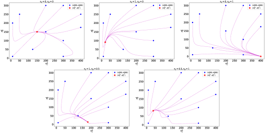
Figure 1: Phase portrait illustrating the dynamics of $(n_{C}^{A},n_{D}^{A})$, with $\beta^{A}$ = $\beta^{K}$ = $0.01$.

To better illustrate this observation, Fig.2 shows the effect of delays on the stable interior state (with stability verified through numerical solutions of Equation (II.1) and (II.2). Left figures depict the impact of delays on the size of $c$ and $D$ populations in adult and juvenile compartments, while right figures focus on the frequency of strategies. When the delay for cooperators is fixed and the delay for defectors is varied, the number of individuals adopting the cooperator strategy in both adult and kindergarten populations increases, while the number of defectors decreases. Consequently, this results in a higher frequency of cooperators in the overall population. For smaller values of $\tau_{D}$, the number of defectors in kindergarten initially exceeds that of cooperators, but this trend reverses at a critical point near $\tau_{D}\approx 0.42$. Therefore at the start of varying the delay for defectors, the frequency of cooperators in kindergarten initially decreases before subsequently increases.

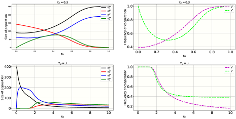
Figure 2: Stationary population sizes and frequencies of cooperation as functions of time delays, numerical solutions of (II.1) and (II.2). $\beta^{A}$ = $\beta^{K}$ = $0.01$.

When the delay for defectors is fixed, and the delay for cooperators is varied, the results are reversed. In this case, all population sizes decrease with increasing $\tau_{C}$, and the frequency of cooperators in both the kindergarten and adult population decline. These findings align closely with those reported in [14, 6], which showed that introducing a time delay for a given strategy is not beneficial. However delay can simultaneously reduce the number of individuals employing both the cooperator and defector strategies.

In the next section, we incorporate stochasticity into our model to explore how delays influence population dynamics in the presence of stochastic fluctuations.

III Markov jump process of the compartment model

Here we study a stochastic model corresponding to replicator dynamics discussed in the previous section. We follow closely Tao and Cressman [5]. In our construction, rates present in replicator equations become now intensities in a Markov jump process, a Markov chain in continuous time and a discrete space of states.

The state of the Markov chain is described by the numbers of players of two strategies of both compartments, $\{n_{i}^{j}\}$, where $i\in\{C,D\}$ and $j\in\{A,K\}$. Intensities of jumps are given in Table 1.

Transition	intensities
$n_{i}^{A}\to n_{i}^{A}+1$	$\frac{n_{i}^{K}}{\tau_{i}}$
$n_{i}^{A}\to n_{i}^{A}-1$	$\beta^{A}N^{A}n_{i}^{A}$
$n_{i}^{K}\to n_{i}^{K}+1$	$n_{i}^{A}\pi_{i}$
$n_{i}^{K}\to n_{i}^{K}-1$	$\frac{n_{i}^{K}}{\tau_{i}}+\beta^{K}N^{K}n_{i}^{K}$

Table 1: Intensities of transitions between states of the Markov chain. The state of the chain at any time $t$ is given by $\{n_{i}^{j}\}$, where $i\in\{C,D\}$ and $j\in\{A,K\}$

Let $\Phi(n_{C}^{A},n_{D}^{A},n_{C}^{K},n_{D}^{K};t)$ be the joint probability distribution for the system to be at a given state the state at time $t$. One can write a standard Master equation,

$$\frac{d\Phi(n_{C}^{A},n_{C}^{A},n_{C}^{K},n_{C}^{K};t)}{dt} =\sum_{i\in C,D}\sum_{j=A,K}(E_{i}^{+,j}-1)\beta^{j}N^{j}n_{i}^{j}\Phi+\sum_{i=C,D}(E_{i}^{-,K}-1)n_{i}^{A}\pi_{i}\Phi$$

$$+\sum_{i==C,D}(E_{i}^{-,A}E_{i}^{+,K}-1)\frac{n_{i}^{K}}{\tau_{i}}\Phi,$$ (III.1)

where

$$E_{i}^{\pm,j}F(n_{i}^{j})=F(n_{i}^{j}\pm 1)$$ (III.2)

One may then derive differential equations for the expected values and other moments of the number of players. However it is impossible to solve such equations. Therefore we will resort to stochastic simulations, we will implement a classic Gillespie algorithm [16].

Let us notice first that our Markov chain has an absorbing state $(0,0,0,0)$. Such a situation is typical in many processes in biological and social models, the Moran process being the classic example. Our focus here is on the long-term behavior of the system under the assumption that the population is not extinct. We will estimate expected values of population sizes and strategy frequencies.

We simulate $1000$ trajectories, with each trajectory consisting of $100,000$ Monte-Carlo steps. The expected value of $n_{i}^{j}$ is then computed as the average over the final $1000$ steps of all trajectories. Similarly, we calculate $\langle x\rangle=\langle\frac{n_{C}^{A}}{N^{A}}\rangle$.

Fig. 3(c) shows that from many initial condition $(30,30,0,0)$, all trajectories converge towards a unique equilibrium, which we refer to as the quasi-stationary state.

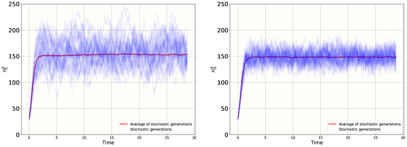
(a) $\tau_{C}=\tau_{D}=0$

(b) $\tau_{C}=0,\tau_{D}=2$

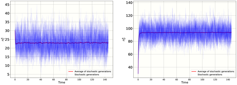
(c) $\tau_{C}=2,\tau_{D}=0$

Figure 3: Single trajectories are represented by blue lines, their averages are shown in red, for three different delay values. $\beta^{A}$ = $\beta^{K}$ = $0.01$ and the initial condition for each trajectory is set to $(30,30,0,0)$

.

First we look at trajectories for different delays. $\beta^{A}$ and $\beta^{K}$ are fixed at $0.01$, and the initial condition for each trajectory is set to $(30,30,0,0)$. Fig. 3(c) presents results of stochastic simulations for three different delays, single trajectories are represented by blue lines, their averages are shown in red. All trajectories remain around the quasi-stationary state for an extended period of time. Since the only absorbing state of this process is $(0,0,0,0)$, the system will eventually reach extinction. However starting from a big initial condition (as indicated in [5], $n_{i}^{A}\geq 20$) and with small $\beta^{A}$ and $\beta^{K}$, the extinction happens in a very long time. Consequently, none of the trajectories in this analysis reach extinction. We observe that expected values of $\langle n_{C}^{A}\rangle$, $\langle n_{D}^{A}\rangle$ and consequently $\langle x\rangle$ depend on delays.

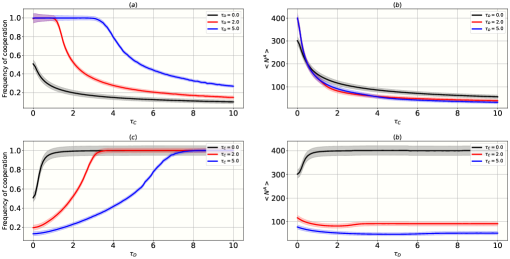
Figure 4: Expected values of the total adult population size and the frequency of cooperation $\langle x\rangle$ at quasi-stationary state as functions of time delays. The value of both $\beta$’s are set to $0.01$.

To examine how delay affects the expected frequency of cooperators and the total population size in the quasi-stationary state, we fixed one delay while varying the other. The results are shown in Fig.4. In panels (a) and (b), the delay for defectors is fixed at three different values ($0$, $2$, and $5$), while the delay for cooperators is varied from $0$ to $10$. In all cases, increasing the delay reduces the expected frequency of cooperators. Furthermore, this delay decreases the total population size, with the decline being more pronounced for cooperators. Conversely, when the delay for cooperators is fixed and the delay for defectors is varied, we observe an increase in $\langle x\rangle$, indicating that the delay of defectors facilitates the emergence of cooperators in the population. However, changes in the total adult population size exhibit a more complex behavior. Depending on the value of $\tau_{C}$, it may increases or initially decrease, then increases.

As observed in Fig. 4, when delays for cooperators and defectors are equal, both $\langle x\rangle$ and $\langle N^{A}\rangle$ exhibit changes. To investigate this further, we set $\tau_{C}=\tau_{D}=\tau$ and vary $\tau$. The results are shown in Fig. 5. When delays are equal for for both strategies and increase, the total population size decreases. This outcome is expected, as individuals spend more time in kindergarten. However, the frequency of cooperators $\langle x\rangle$ increases with increasing delay. This observation contrasts with previous findings in [14, 6] where in deterministic models there are no changes in frequencies of strategies. Here strategy-independent delays promote the cooperative behavior in our stochastic model. An intriguing observation is that the impact of introducing the same delay for both strategies is different in the deterministic model described in the previous section and in the stochastic one.

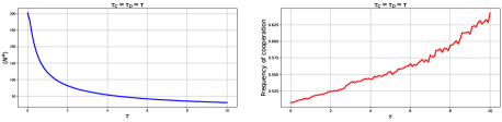
Figure 5: Expected values, $\langle N^{A}\rangle$ and $\langle x\rangle$, in the quasi-stationary state as functions of delays equal for both strategies. $\beta$’s are set to $0.01$.

Below we examine the case where delays are not equal but are very close to each other. Previous studies have shown that when the delay associated with a given strategy is larger than the delay of the other one, then it tends to disadvantage that strategy. However, in Fig.6, we observe that for a game with an interior stationary state at $0.5$ (in the absence of delays), even a slightly larger delay for $\tau_{C}$ compared to $\tau_{D}$ promotes cooperation. In such cases, the stationary frequency of cooperators exceeds $0.5$. Of course, this effect holds only when $\tau_{C}$ is slightly larger than $\tau_{D}$. When the difference becomes significant, and $\tau_{C}$ is sufficiently large, similar to what is seen in the deterministic, it negatively impacts cooperation, reducing the cooperator frequency below $0.5$. The value of $\tau_{C}$ (where $\tau_{C}>\tau_{D}$) at which cooperation is still favored depends on the value of $\tau_{D}$. For instance, in Fig.6, when $\tau_{D}=2$, cooperation is favored up to $\tau_{C}=2$. However, when $\tau_{D}=5.0$, cooperation can be favored up to $\tau_{C}=5.35$, indicating a larger possible difference between the delays.

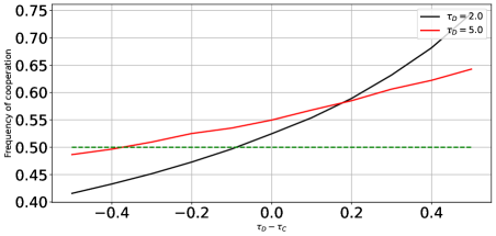
Figure 6: Cooperation frequency in the quasi stationary state as a function time delays difference. $\beta$’s are set to $0.01$.

The observed behavior differences between deterministic and corresponding stochastic dynamics are noteworthy. To better understand these discrepancies and uncover their origins, we analyze the time evolution of the number of cooperators and defectors, as well as the transition probabilities Fig.7. These probabilities are calculated as the intensity of a given transition divided by the sum of all intensities at a current state of the system, where $\tau_{C}=\tau_{D}=\tau$. The curve presented in Fig.7 is the average of $1,000$ trajectories. Starting from identical initial conditions, we observe that for $\tau=1$, the number of cooperators grows faster than that of defectors, whereas for $\tau=10$, the probability that the number of defectors decreases surpasses that of cooperators. This explains why, in the quasi-stationary state, the frequency of cooperators exceeds that of defectors, in contrast to deterministic replicator dynamics where their frequencies are equal.

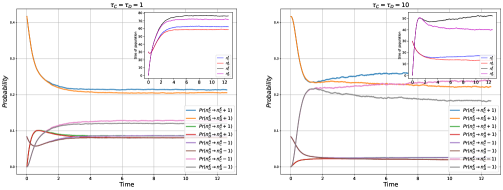
Figure 7: Time evolution of the number of strategies and the probability of transition for strategy independent delays. The probability of a transition is the intensity of that transition divided by the sum of all intensities at a current state of the system. Each curve is the average of 1,000 trajectories.

As $\tau$ increases, the time juveniles spend in the kindergarten is extended, resulting in fewer individuals transitioning to the adult population. The intensity of the transition $n_{i}^{K}\to n_{i}^{K}+1$, which depend on payoff values, reveals that a reduced number of cooperators negatively impacts defectors and cooperators. However, fewer defectors benefit cooperators more than defectors themselves. Over time, the probability of strategy growth within the kindergarten phase decreases, with cooperators experiencing a slower reduction compared to defectors. Simultaneously, the probability of death in the kindergarten phase, which depends on population size, increases but more for cooperators, given their larger numbers in kindergarten relative to defectors. Together, these dynamics explain why cooperators initially increase more rapidly for smaller $\tau$ or decline more gradually for larger $\tau$, before the population reaches its quasi-stationary state.

Fig.8 illustrates effects of both delays on the frequency of cooperators in the quasi-stationary state. Clearly, for a fixed $\tau_{D}$, increasing $\tau_{C}$ leads to a decrease in the level of cooperation. Conversely, for a fixed $\tau_{C}$, increasing $\tau_{D}$ results in the opposite trend, with cooperation levels rising. An interesting observation is that the parameter $\beta$ can also influence the frequency of cooperation, even when delay values remain constant. This can be explained similarly to the case of equal time delays: $\beta$ represents an increased death rate, which reduces the number of both cooperators and defectors in the population. A smaller population size can favor cooperators, thereby increasing their frequency in the stationary state.

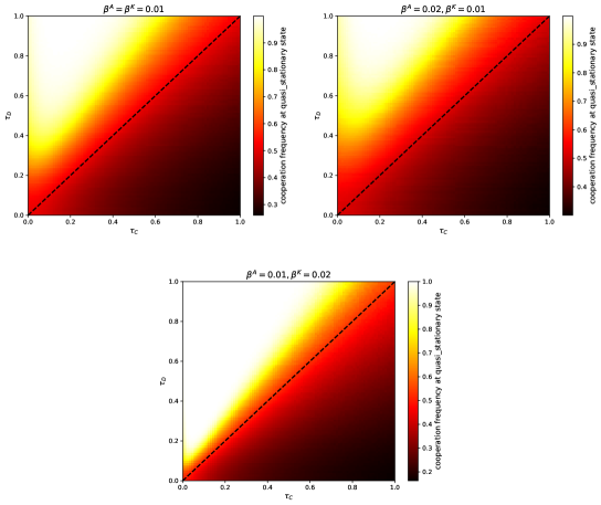
Figure 8: Effect of $\tau_{C}$ and $\tau_{D}$ on the frequency of cooperation in the adult population in the quasi-stationary state for various values of $\beta^{A}$ and $\beta^{K}$.

IV Discussion

We studied effects of time delays in deterministic and stochastic models of the Snowdrift game. We combined ideas and constructions of [5] and [6] and presented a compartment model with deaths which correspond to logistic suppression associated with the carrying capacity.

In the replicator dynamics, the stationary states of population sizes and strategy frequencies depend continuously on time delays represented by transition rates between compartments. In the corresponding birth-death Markov jump processes we observe a novel behavior, time delays are beneficial for the cooperation strategy; frequencies of strategies depend continuously also for equal delays of both strategies. This phenomenon is not observed in the corresponding deterministic model. For strategy-independent delays, stationary states of frequencies are equal to those of classical replicator dynamics without time delays.

Somewhat analogous behavior has been observed recently in random walks with asymmetric time delays. It was observed there that we may reverse effects of time delays by a symmetric transformation of fitness functions and then the time delay of a given strategy increases its frequency in the stationary distribution [20].

It is worth to mention here that a logistic suppression was directly incorporated in replicator dynamics in [18, 18, 19]. It is an interesting problem to extend the authors models by adding time delays and intrinsic noise.

In general it is important to study the joint effects of time delays and stochasticity. Some results we presented in [21, 20, 23].

Appendix A

As mentioned in the main text, the deterministic equations differ when either one or both delays are zero. If the delay for a particular strategy is zero, it implies that new juveniles, born in proportion to the payoff, are immediately added to the adult population. Below, we present the equations for the various delay scenarios.

• $\tau_{C}=\tau_{D}=0$:

  $$\begin{cases}\frac{dn_{C}^{A}}{dt}=n_{C}^{A}\pi_{C}-\beta^{A}N^{A}n_{C}^{A}\\ \frac{dn_{D}^{A}}{dt}=n_{D}^{A}\pi_{D}-\beta^{A}N^{A}n_{D}^{A}\end{cases}$$ (A.1)

  $$\begin{cases}\frac{dx}{dt}=x(1-x)(\pi_{C}-\pi_{D})\\ \frac{dN^{A}}{dt}=N^{A}(\bar{\pi}-\beta^{A}N^{A})\end{cases}$$ (A.2)

• $\tau_{C}=0,\tau_{D}>0$:

  $$\begin{cases}\frac{dn_{C}^{A}}{dt}=n_{C}^{A}\pi_{C}-\beta^{A}N^{A}n_{c}^{A}\\ \frac{dn_{D}^{A}}{dt}=\frac{n_{D}^{K}}{\tau_{D}}-\beta^{A}N^{A}n_{D}^{A}\\ \frac{dn_{D}^{K}}{dt}=n_{D}^{A}\pi_{D}-\beta^{K}{(n_{D}^{K})}^{2}-\frac{n_{D}^{K}}{\tau_{D}}\end{cases}$$ (A.3)

  $$\begin{cases}\frac{dx}{dt}=x\big{(}(1-x)\pi_{c}-\frac{N^{K}}{\tau_{D}}\big{)}\\ \frac{dN^{A}}{dt}=N^{A}\big{(}x\pi_{c}-\beta^{A}N^{A}\big{)}+\frac{N^{K}}{\tau_{D}}\\ \frac{dN^{K}}{dt}=N^{A}(1-x)\pi_{D}-\frac{N^{K}}{\tau_{D}}-\beta^{K}{N^{K}}^{2}\end{cases}$$ (A.4)

• $\tau_{C}>0,\tau_{D}=0$:

  $$\begin{cases}\frac{dn_{D}^{A}}{dt}=n_{D}^{A}\pi_{D}-\beta^{A}N^{A}n_{D}^{A}\\ \frac{dn_{C}^{A}}{dt}=\frac{n_{C}^{K}}{\tau_{C}}-\beta^{A}N^{A}n_{C}^{A}\\ \frac{dn_{C}^{K}}{dt}=n_{C}^{A}\pi_{C}-\beta^{K}{(n_{C}^{K})}^{2}-\frac{n_{C}^{K}}{\tau_{C}}\end{cases}$$ (A.5)

  $$\begin{cases}\frac{dx}{dt}={(1-x)}^{2}\pi_{D}-\frac{N^{K}x}{\tau_{C}}\\ \frac{dN^{A}}{dt}=N^{A}\big{(}(1-x)\pi_{D}-\beta^{A}N^{A}\big{)}+\frac{N^{K}}{\tau_{C}}\\ \frac{dN^{K}}{dt}=N^{A}x\pi_{C}-\frac{N^{K}}{\tau_{C}}-\beta^{K}{N^{K}}^{2}\end{cases}$$ (A.6)

• $\tau_{C}=\tau_{D}=\tau$:

  $$\begin{cases}\frac{dn_{C}^{A}}{dt}=\frac{n_{C}^{K}}{\tau}-\beta^{A}N^{A}n_{C}^{A}\\ \frac{dn_{D}^{A}}{dt}=\frac{n_{D}^{K}}{\tau}-\beta^{A}N^{A}n_{D}^{A}\\ \frac{dn_{C}^{K}}{dt}=n_{C}^{A}\pi_{C}-\beta^{K}N^{K}n_{C}^{K}-\frac{n_{C}^{K}}{\tau}\\ \frac{dn_{D}^{K}}{dt}=n_{D}^{A}\pi_{C}-\beta^{K}N^{K}n_{D}^{K}-\frac{n_{D}^{K}}{\tau}\end{cases}$$ (A.7)

  $$\begin{cases}\frac{dx}{dt}=\frac{N^{K}}{N^{A}}\big{(}\frac{y(1-x)-x(1-y)}{\tau}\big{)}\\ \frac{dy}{dt}=\frac{N^{A}}{N^{K}}\big{(}x\pi_{C}-y\bar{\pi}\big{)}\\ \frac{dN^{A}}{dt}=\frac{N^{K}}{\tau}-\beta^{A}(N^{A})^{2}\\ \frac{dN^{K}}{dt}=N^{A}\bar{\pi}-\frac{N^{K}}{\tau_{C}}-\beta^{K}{N^{K}}^{2}\end{cases}$$ (A.8)

The key observation in our paper is that the qualitative behavior is different for deterministic and stochastic dynamics when delays for both strategies are equal. We solve the system of equations (A.8) for the stationary state by setting all derivatives to zero. From the first equation we get $x^{*}=y^{*}$. Substituting this into the second one we obtain $\frac{N^{A}}{N^{K}}x(1-x)(\pi_{C}-\pi_{D})=0$. For the general Snowdrift game we get the interior stationary state of the frequency of adult cooperators $x^{*}=1-r$, where $r=\frac{c}{2b-c}$ for $\pi_{C}=\pi_{D}$. We conclude that strategy-independent delays do not shift stationary states of frequencies.

References

- [1] P. D. Taylor and L. B. Jonker, Evolutionarily stable strategy and game dynamics, Math. Biosci. 40, 145 (1978).
- [2] J. Hofbauer, P. Shuster, and K. Sigmund, A note on evolutionarily stable strategies and game dynamics, J. Theor. Biol. 81, 609 (1979).
- [3] J. Hofbauer and K. Sigmund, The Theory of Evolution and Dynamical Systems (Cambridge University, 1988).
- [4] J. Weibull, Evolutionary Game Theory (MIT Press, Cambridge MA, 1995).
- [5] Y. Tao and R. Cressman, Stochastic fluctuations through intrinsic noise in evolutionary game dynamics, Bull. Math. Biol. 69: 1377–1399 (2007).
- [6] M. Fic, F. Bastia, J. Miȩkisz, and C. Gokhale, Compartment model of strategy-dependent time delays in replicator dynamics, arXiv:2409.01116 (2024).
- [7] Y. Tao and Z. Wang, Effect of time delay and evolutionarily stable strategy, J. Theor. Biol. 187, 111 (1997).
- [8] J. Alboszta and J. Miȩkisz, Stability of evolutionarily stable strategies in discrete replicator dynamics with time delay, J. Theor. Biol. 231: 175 (2004).
- [9] I. Györi and G. Ladas, Oscillation Theory of Delay Differential Equations with Applications (Clarendon, Oxford, 1991).
- [10] K. Gopalsamy, Stability and Oscillations in Delay Differential Equations of Population (Springer Science+Business Media, 1992).
- [11] Y. Kuang, Delay Differential Equations with Applications in Population Dynamics (Academic Press, Boston, 1993).
- [12] T. Erneux, Applied Delay Differential Equations (Springer Science+Business Media, 2009).
- [13] M. Bodnar, J. Miȩkisz, and R. Vardanyan, Three-player games with strategy-dependent time delays, Dyn. Games Appl. 10, 664 (2020).
- [14] J. Miȩkisz and M. Bodnar, Evolution of populations with strategy-dependent time delays, Phys. Rev E 103, 012414 (2021).
- [15] J. Miȩkisz, J. Mochamadichamgavi, and R. Vardanyan, Small time delay approximation in replicator dynamics, arXiv:2303.08200 (2023).
- [16] D. T. Gillespie, Exact stochastic simulation of coupled chemical reactions, J. Phys. Chem. 81: 2340–2361 (1977).
- [17] K. Argasiński and M. Broom, Ecological theatre and the evolutionary game: how environmental and demographic factors determine payoffs in evolutionary games, J. Math. Biol. 67: 935-962 (2013).
- [18] K. Argasiński and M. Broom, Interaction rates, vital rates, background fitness and replicator dynamics: how to embed evolutionary game structure into realistic population dynamics, Theory in Biosciences 137: 33-50 (2018).
- [19] K. Argasiński and M. Broom, Evolutionary stability under limited population growth: Eco-evolutionary feedbacks and replicator dynamics, Ecological Complexity 34: 198-212 (2018).
- [20] K. Łopuszański and J. Miȩkisz, Random walks with assymetric time delays, Phys. Rev. E 105: 064131 (2022).
- [21] J. Miȩkisz, M. Matuszak, and J. Poleszczuk, Stochastic stability in three-player games with time delays, Dynamic Games and Applications 4: 489-498 (2014).
- [22] J. Miȩkisz and S. Wesołowski, Stochasticity and time delays in evolutionary games, Dynamic Games and Applications 1: 440-448 (2011).
- [23] J. Mohamadichamgavi and M. Broom, The impact of time delays on mutant fixation in pairwise social dilemma games, Proceedings A 480: 2024019 (2024).