Towards influence centrality: where to not add an edge in the network?
Abstract
In this work, we consider a strongly connected group of individuals involved in decision-making. The opinions of the individuals evolve using the Friedkin-Johnsen (FJ) model. We consider that there are two competing ‘influencers’ (stubborn agents) vying for control over the final opinion of the group. We investigate the impact of modifying the network interactions on their respective control over the final opinions (influence centrality). We use signal flow graphs (SFG) to relate the network interactions with the influence that each ‘influencer’ exerts on others. We present the sufficient conditions on the edge modifications which lead to the increase of the influence of an ‘influencer’ at the expense of the other. Interestingly, the analysis also reveals the existence of redundant edge modifications that result in no change in the influence centrality of the network. We present several numerical examples to illustrate these results.
I INTRODUCTION
An influential node in a social network holds the ability to drive the opinions of others in the networks. In a network with two or more such agents, increasing the influence of one over the other has applications in political campaigns, the promotion of specific brands, combating fake news, etc. Such applications rely on suitably varying the influence of a chosen node. Increasing a node’s centrality is an intriguing problem that has mainly been explored for PageRank in [1, 2] to increase the visibility of a webpage. Recent works have also explored the problem of increasing closeness [3] and betweenness centralities [4] of a node with the objective makes it an efficient spreader of information.
In social networks, the influence/centrality of a node, along with the network topology, also depends on the underlying process of opinion aggregation [5]. Several models have been proposed in the literature [6] that analyse the effect of information aggregation on opinion formation. The FJ model, proposed in [7], is popular due to its simplicity and analytical traceability. In the FJ framework, there are stubborn agents who are reluctant to change their opinions and turn out to be influential. Their impact on opinion formation is quantified by the influence centrality measure proposed in [8]. In the FJ framework, a random-walk-based interpretation for the final opinions of the agents is proposed in [9] and [10] for undirected and directed graphs, respectively.
Relevant literature: Using the relation between the network topology and the final opinions, network modifications such as edge addition/removal/reweighing of edges are used in the FJ framework to achieve the objectives such as polarization minimisation [11, 12], reduction of exposure to harmful content [13], opinion maximization [14], etc. In general, such network optimisation problems are combinatorial and, therefore, intractable. They employ greedy heuristics due to the non-convex objective functions [12, 15], NP-hardness of the problem [10, 13] etc. Recent works [12] and [16] use network properties such as Cheeger’s constant and the degree of nodes to arrive at closed-form solutions of the impact of an edge addition on the reduction in polarisation and conflict, respectively. Based on this formulation, a disagreement-seeking heuristic is proposed in [12] that reduces polarisation by increasing the edge weights of disagreeing nodes. The GAMINE algorithm presented in [13] reduces exposure to malicious content by utilising the weak connectivity of graphs. It substitutes an edge with to increase connectivity with safe node(s) that do not have any exposure to harmful content. An equivalent approach is implemented in [17] to achieve opinion maximisation. The impact of edge modifications is explored in [18] in the optimisation of controllability grammian-based metrics for an LTI system. A better understanding of the network topology is, therefore, useful in proposing heuristics for network optimisation problems.
In this work, there are agents in a strongly connected network whose opinions evolve using the FJ model; two of the agents are stubborn and are competing to maximise their own influence. Our primary objective is to analyse the impact of arbitrary edge modifications on the influence centrality of the network. The proposed analysis has applications in network optimisation problems especially with the objective of opinion maximisation/minimisation [17] and the reduction of exposure to malicious content [13]. In this paper, we consider a modification that mimics the ‘feed calibration’ on social media: an edge is added and the edge weight of an existing edge of is reduced such that the in-degree of remains constant [19]. Utilising a graphical SFG-based approach, we present topological conditions on the edge modifications that can change the influence centrality of the network in a desired way, independent of the modified edge weights. Our key contributions are as follows:
-
•
We present the sufficient conditions under which an edge modification in the network is redundant. Identifying such edge modifications is relevant to avoid uneconomical modifications in practical scenarios.
-
•
Secondly, we present sufficient conditions on the network topology under which an edge modification increases the influence centrality of either of the two stubborn agents irrespective of edge weights.
The paper has been organised as follows: Sec. II discusses the relevant preliminaries. We formally define the problem of examining the impact of edge modification in Sec. III. Sec. IV utilises the SFGs to relate an edge modification with the change in influence centrality. Sec. V presents the topology-based conditions that determine the impact of edge modification. Sec. VI illustrates the results using a suitable example. In Sec. VII, we conclude with insights into the possible future research directions.
II Preliminaries
II-A Graph Preliminaries
A network of agents defined as where is the set of nodes representing the agents in the network, is the set of ordered pair of nodes called edges which denote the communication topology of the network. An edge denotes the information flow from agent to agent . The in-neighbours of an agent is defined as and the out-neighbours of is defined as . A source is a node without in-neighbours and a sink is a node without out-neighbours. The matrix is the weighted adjacency matrix of network whose entries if an edge else . The in-degree of a node is defined as .
A path is an ordered sequence of nodes in which every pair of adjacent nodes produces an edge that belongs to the set . A forward path is one where none of the nodes is traversed more than once. A feedback loop is a forward path where the first and the last nodes coincide. The path gain and loop gain are the product of the edge weights of edges forming the path and loop, respectively. A network is strongly connected if each node in the network has a directed path to every other node.
II-B FJ model
The FJ model is an extension of DeGroot’s model that takes stubborn behaviour among agents into account. An agent exhibits stubborn behaviour if it is reluctant to change from its initial position or opinion. The opinions of agents in a network which are governed by the FJ model evolve as follows,
| (1) |
where denotes the opinion of agents in at the instance, is a row-stochastic weighted adjacency matrix, is a diagonal matrix with denoting the degree of stubbornness of agent . An agent is a stubborn agent if .
Lemma 1
[7] When the underlying network is strongly connected and such that for at least one , the following conditions hold:
-
•
at steady state, the opinions of the agents converge to,
(2) where and .
-
•
the matrix is row-stochastic
II-C Signal Flow Graphs and Index Residue Reduction
An SFG is a graph with each node is associated with state . Each state satisfies a linear equation of the form ; where is the branch gain of branch denoting the dependence of state on state . In an SFG, one or more sources may exist. Note that the state associated with a source is independent of any other state while it directly or indirectly affects the states associated with the other nodes in the SFG.
In general, the SFGs are used to determine the effect of inputs on various states in the system. Each input forms a source in the SFG. The gain of the SFG is defined as the signal appearing at the sink per unit signal applied at the source [20]. In the absence of loops, the gain of SFG for a pair of source and sink is the summation of path gains of all forward paths from the source to the sink in . On the other hand, if an SFG has a self-loop with gain it is replaced by a branch of gain and the gain of the SFG is calculated. However, in the presence of loops consisting of two or more nodes, additional terminologies are required which are defined as follows.
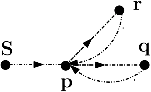
In an SFG, a node can be split into two nodes and , such that node is connected with all the outgoing branches of and is connected to all incoming branches of . The smallest set of nodes that must be split to remove all the loops in the graph is denoted by . The nodes in are referred to as index nodes. In Fig. 1, we split a node in given in Fig. 1(a). This results in an SFG without any loops shown in Fig. 1(b). Therefore, it follows that is an index node. Note that the index nodes of a graph need not be unique.

The gain of an SFG with loops is determined by using index-residue reduction of the SFG. A reduced SFG is formed that has nodes consisting of sources, sinks and index nodes of . The nodes retained in are called residual nodes, and the residual path is a path in that starts from a residual node to another residual node or (itself) without passing through any other residual node. A branch exists in if a residual path exists in from an index node or a source to an index node or a sink . The non-residual nodes are the nodes in other than the residual nodes. The branch gain is equal to the sum of path gains of the residual paths in . Next, the self-loops, if any, are converted into branches by the aforementioned procedure. If the reduced graph does not contain any loops, we determine the gain of the sources. Otherwise, the index-residue reduction is performed iteratively until the reduced graph does not contain any loops.
III Problem Statement
The FJ model is one of the most well-studied models in the literature of mathematical sociology and opinion dynamics. This model introduced stubborn behaviour in agents, which results in disagreement, the commonly occurring outcome of social interactions. In a network of agents, the term influential simply refers to an agent having a say in the final opinions of the agents in the network. Interestingly, when the opinions of the agents evolve by the FJ model, only the stubborn agents are influential [7]. Formally, we define an influential agent in the FJ framework as follows:
Definition 1
A stubborn agent is said to influence another agent , when its initial opinion contributes to the final opinion of agent .
Once the influential agents are identified, a natural question arises about their impact on the other agents in the network. The influence centrality measure, proposed in [8], quantifies the contribution of stubborn agent(s) on the final opinions of the agents in the framework of FJ model. Mathematically, it is defined as follows:
| (3) |
where denotes the influence centrality measure of agents in the network whose entry gives the degree of influence of a stubborn agent . The influence centrality measure satisfies , implying that if the influence of a stubborn agent increases, there exists another stubborn agent whose influence decreases.
It is well known that the influence centrality measure depends on the degree of stubbornness of all the agents and the network topology [7, 9]. In practical applications such as the mitigation of the spread of fake news or promoting certain brands to wider target audiences, it might be desirable to make one agent (or brand) more influential (or popular) than the others. Therefore, harping on the critical role of network topology on the degree of influence, we analyse the effect of edge modifications to suitably alter a stubborn agent’s influence in a strongly connected network.
III-A Implications of edge modifications in social networks
The addition of a directional edge between two nodes and in a social network can be interpreted as a suggestion for to establish a friendship with and follow its posts. Adding new friends on social media leads to a phenomenon of ‘feed alteration’ where the visibility of posts from existing friends may decrease to accommodate the content from the newly added ones. Therefore, the added edge is accommodated by a reduction in edge weight of an existing edge, say such that the in-degree of remains constant. Formally, we define an edge modification as:
Definition 2
Given distinct nodes , and , an edge modification is the addition of an edge and the reduction of edge weight of the existing edge such that the in-degree of remains constant which implies:
| (4) |
where is the weight of the edge in and , are the weights of the edges and , respectively, after the edge modification such that and .
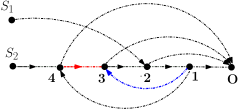
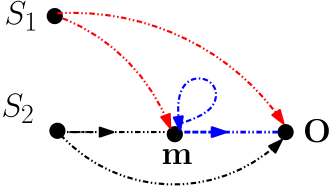
Note that, throughout the paper, the added edge is indicated by a blue arrow and the edge whose weight is reduced is represented by a red arrow.
Example 1

III-B Primary objectives
In this paper, our primary objective is to analyse the impact of edge modifications on the degree of influence of the stubborn agents. For simplicity, we consider only two agents in the network to be stubborn. Therefore, an increase in the influence of either of the stubborn agents results in a decrease in the influence of the other. Such a framework captures real-world contests for influence like in a bipartisan political system or a duopoly of firms. Mathematically, we are interested in arriving at sufficient conditions on the network topology such that the edge modification results in a suitable change in the degree of influence of only either one of the stubborn agents.
IV Influence and signal flow graphs
Consider a network of agents whose opinions evolve by eqn. (1) when only two agents in the network are stubborn. In the given framework, the final opinions of the agents in the network satisfy the following set of linear equations,
| (5) |
The average of final opinions of agents, denoted by , relates to the influence centrality measure by the following equations.
| (6) |
In the given framework, depends only on the initial opinions of stubborn agents. It follows from eqn. (6) that the contribution of a stubborn agent in is equal to its degree of influence . We concatenate eqns. (5) and (6) to get the following relation.
| (7) |
This steady-state relation can be expressed graphically using an SFG. Such a representation is useful in visualising how the final opinions of different agents are related to one another. (See [21] for a detailed description of the use of SFG in influence analysis.)
In the given framework, the SFG , derived using (7), is composed of the following nodes:
-
•
Each of the first nodes represent the final opinion of the agent in the network.
-
•
The next two nodes correspond to the initial opinion of the stubborn agent in . These nodes form sources and in .
-
•
The last node is associated with average final opinion . It forms a sink in and is denoted by .
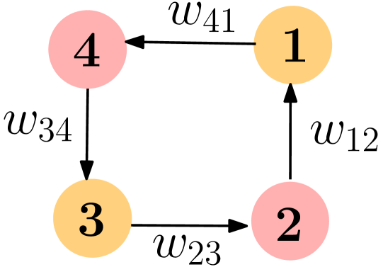
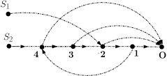
where . We use the relations in eqn. (7) to form the branches in . A branch in has branch gain for . Further, sources and in have out-going branches with branch gains being their degrees of stubbornness. The sink in has an incoming branch from each node in with branch gain where . Using the given procedure, the SFG constructed for a strongly connected network in Fig. 2(a) is shown in Fig. 3(a).
The degree of influence of a stubborn agent is the gain of the SFG for source and sink where is associated with , and . In this paper, our aim is to determine the change in the degree of influence resulting from an edge modification in and attribute its underlying causes. Therefore, we use the index residue reduction (detailed in Appendix A) to further simplify the SFG.
IV-A Impact of edge modification in on
It is simple to observe that the addition of an edge in the network is equivalent to the addition of a branch in the SFG such that . Similarly, the reduction of edge weight of in results in the reduction of branch gain of in where . It can be determined that the in-degree of any node in except sources is equal to , which further remains constant despite the edge modification. The impact of edge modification in on is demonstrated in Example 2.
Example 2
For the network in Fig. 2(a), we construct its SFG as shown in Fig. 3(a). The network in Fig. 2(b) is obtained after an edge modification . Equivalent changes are reflected in the SFG as shown in Fig. 3(b).
IV-B Index nodes and the permissible edge modifications
The analysis of the impact of edge modifications is extremely useful in real-world applications, an example being the marketing of products in appropriate or selective regions within a network. However, the task becomes increasingly challenging as the networks become more dense with edges. Keeping this in mind, in this paper, we consider a subset of strongly connected networks that adhere to the following assumption.
Assumption 1
Given a network , there exists a node that occurs in every loop in the except the self-loops.
Due to Assumption 1, an interesting property arises for the underlying SFG corresponding to the network . In general, any SFG can be subjected to a procedure known as the index residue reduction. This procedure starts with the identification of the index nodes in the network. Loosely speaking, an index node is one which is associated with one or more loops in the network; interestingly, the network loses its cyclicity in the absence of all of its index nodes. The complete procedure of the identification of index nodes and the index residue reduction is detailed in Sec. II-C.
Remark 1
For a given network that satisfies Assumption 1, the corresponding SFG has only one index node.
Example 3
The network shown in Fig. 2(b) has two loops and . Nodes and are common in both the loops such that if we split one of the corresponding nodes in the SFG , then becomes acyclic. Thus, either one of or can be chosen as an index node.
Lemma 2
In a network satisfying Assumption 1, the non-residual nodes (the nodes except the index node, sink and sources) in can be distributed into disjoint sets of levels where . A node in a set satisfies the following conditions on its in-neighbours:
-
1.
the nodes in the set are allowed to be its in-neighbours, and,
-
2.
it must have at least one in-neighbour from .
Proof:
During the construction of the SFG , WLOG, we choose to make the index node, say , as the first node. The reason is its connectivity with the other nodes. Due to the Assumption 1, the non-residual nodes cannot form a loop that does not have node . If a node in has in-neighbours from a node in set , then the non-residual nodes may form a loop amongst themselves. This violates Assumption 1 leading to a contradiction. Thus, condition (1) holds. Condition (2) holds so that each non-residual node belongs to a unique set . ∎
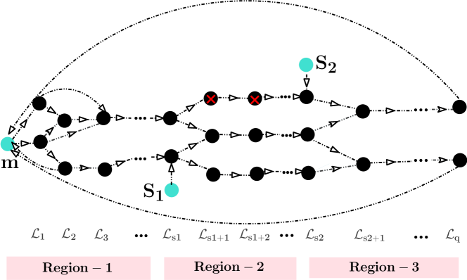
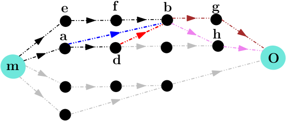
The non-residual nodes in can be distributed in levels as shown in Fig. 4. In , the nodes highlighted in blue in Fig. 4, denote the residual nodes. For ease of visualisation, a source in associated with the initial opinion of a stubborn agent is placed in the same level set as the node associated with the final opinion of the stubborn agent. The source whose appearance precedes the other one in the levels is termed as and the other one is referred to as . The sets , are the ones which contain a node with an incoming edge from and , respectively. Note that the sink is omitted in Fig. 4 to avoid confusion.
An important point to note is that the distribution of nodes into levels sets depends on the choice of the index node as explained next.
Example 4
We distribute the non-residual nodes of the SFG in Fig. 3(b) into level sets. We know from Example 3 that the SFG has nodes and as eligible index nodes. We distribute the non-residual nodes of the SFG by considering node as the index node in Fig. 5(a) and by considering node as the index node in Fig. 5(b). Comparing the Figs. 5(a) and 5(b), we observe that the members of level sets differ with the choice of the index node. Furthermore, note that in Fig. 5(a), corresponds to the initial opinion of and corresponds to the initial opinion of . On the other hand, in Fig. 5(b), the vice-versa occurs.
Example 4 illustrates the role of the index node in the distribution of nodes into level sets. Next, we present the conditions for permissible edge modifications in this framework. Throughout this work, we consider the edge modification applied to a network satisfies the following assumption.
Assumption 2
Given a network , an edge modification is permissible if the modified network satisfies Assumption 1.
Assumption 2 implies that an edge modification is permissible only when the modified network has atmost one index node. We can visualise the conditions for a permissible edge modification in terms of the level sets defined for a given index node . Due to the edge addition of where and , two cases might arise (i) and (ii) . In the first case, the edge addition is always permissible because conditions in Lemma 2 hold and continues to be the index node. On the other hand, when , it may result in the formation of a loop without the index node , implying is no longer the index node participating in every loop in the network. Therefore, such edge addition is permissible only when another eligible index node exists such that the Assumption 1 holds. Having explored the impact of the edge modifications on , we analyse their impact on the influence centrality of a network. We show that the use of the SFGs largely simplifies the analysis in the given framework.
V Impact of edge Modifications on Influence
As discussed before, in this paper, we consider a strongly connected network consisting of two stubborn agents. Our primary objective is to analyse the change in the influence of the stubborn agents due to permissible edge modifications. A natural question that arises is: which edge modifications in the network would increase the influence of a selected stubborn agent over the other? In this section, we try to answer this question through the following results.
Definition 3
A node is said to have a direct path from a node , if a path exists in which does not pass through the index node for such that both and are not residual nodes.
If both and are residual nodes in , then a path that does not pass through is a residual path and not a direct path.
Theorem 1
The proof of Theorem 1 is presented in Appendix B. We use the level sets to visualise the conditions given in Theorem 1. As shown in Fig. 4, the nodes in can be distributed in three regions: (1) the nodes from the sets to the set including , (2) the nodes in sets from to the set and (3) the nodes in sets from to .
For a permissible edge modification such that and lie in region , it follows from Lemma 2 that every path from the sources and passes through . Thus, the condition in Theorem 1 holds, and such edge modifications are redundant. Even in regions and , there may exist certain nodes that do not have a path from without passing through . For example, observe the nodes in Fig. 4 in the region marked with red crosses. For such and also, the is also redundant. Since no constraints are imposed on the position of , it can lie in any region as long as is a permissible edge addition. It follows from Theorem 1 that edge modifications such that both and lie in region are redundant. Next, we consider the edge modifications where either one of or lies in the region and has a direct path from .
Theorem 2
Consider a strongly connected network where an edge modification is applied such that the Assumptions 1 and 2 hold. Additionally, let the following conditions hold for an index node in :
-
•
does not have a direct path from any of the sources.
-
•
has at least one direct path from a source
The influence of the stubborn agent corresponding to decreases under these conditions. If the nodes and are interchanged, then the influence of the stubborn agent corresponding to increases.
The proof for the Theorem 2 is presented in Appendix B.
Remark 2
Intuitively, an edge modification such that and have no direct paths from and is redundant because the effect of change gets distributed among both the sources. On the other hand, when has a direct path from , and does not have a direct path from any source. Then, the newly added edge lies on forward path(s) only from , while the reduced edge lies on paths from both and . Therefore, it follows that the influence of decreases leading to an increase in the influence of .
VI An Illustrative example
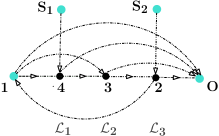
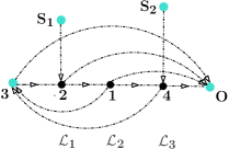
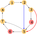
Consider the network shown in Fig. 6(a) where agents and are stubborn. We assume has no self-loops and the weight of each edge is equal. The degree of stubbornness of and is and , respectively. The degree of influence is determined using eqn. (3), turns out to be and . The nodes and in are eligible to be the index nodes. We choose as the index node and introduce an edge modification shown in Fig. 6(b). The weight of the added edge is . In , nodes and do not have direct paths from either of the sources (because in every path from stubborn agents or to agents or passes through ). The degree of influence in the modified network is unchanged and turns out to be and .
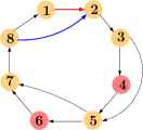
Another permissible edge modification is applied to , as shown in Fig. 6(d). The weight . Note that node is no longer an index node. However, for the choice of node as the index node, the Assumption 2 holds, and the nodes , do not have direct paths from sources. The degree of influence of the modified network verifies that the edge modification is redundant as and .
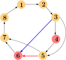
Next, we make an edge modification with in the network . Consider as index node, the node does not have a direct path from sources but has a direct path from associated with stubborn agent . Therefore, according to Theorem 2, the influence of stubborn agent decreases and that of increases. The degree of influence of the modified network is and . Hence, verified.
VII CONCLUSIONS
In this paper, we examine the impact of edge modifications on the influence of the stubborn agents in a network governed by the FJ model. We propose to construct an SFG that relates the influence of the stubborn agents to the network interactions using the steady-state behaviours. Thereafter, the SFG is reduced to a directed acyclic graph using the index residue reduction. Such a reduction allows for an easy determination of the change in the influence of the agents. For a class of strongly connected networks, this procedure allows us to re-structure the SFG such that all the nodes are distributed into level sets. Depending on the locations of the stubborn agents, the level sets are further classified into three regions as shown in Fig. 4. Through rigorous analysis, we show that for edge modifications carried out in region , no change occurs in the influence of any of the stubborn agents. Hence, we know where not to add an edge in the network. We also present the suitable edge modifications in regions and which can increase/reduce the influence of a desired stubborn agent.
The proposed graphical solution is simple, yet can be extremely useful in minimising energy/expenses in practical applications. Further, the set of feasible edge modifications can be substantially reduced through this approach; making it more tractable than optimisation-based frameworks. However, the topological conditions for ensuring non-redundant edge modifications still need to be explored in regions and . In future, we also plan to analyse the scenario of multiple stubborn agents competing for influence and also extend our results to a wider class of networks.
APPENDIX A
VII-A Index Residue Reduction of the SFG
The SFG of a network satisfying Assumption 1 has only one index node. Therefore, we apply the index-residue reduction procedure on to determine its gain. First, we replace each self-loop in with an equivalent branch. This results in an intermediary graph , which has the same nodes and edges as . However, the branch gain of any edge in becomes if had a self-loop in . Now, we further reduce the network to by index residue reduction. The network contains only the residual nodes that include the index node , the sources and and the sink in . For a branch in , the branch gain is the summation of path gains of residual paths from in . The self-loop at in is replaced with a branch of gain .

The gain of the SFG for source and sink is the sum of the path gains of the forward paths from to in , given by,
| (8) |
where is the influence centrality of stubborn agent when is associated with .
Appendix B
Proof of Theorem 1: Since the edge modification in is equivalent to the edge modification in , henceforth, we examine the consequences of altering the network in . We use the index residue reduction of the SFG , presented in Appendix-A, to determine the change in the influence of stubborn agents. It follows from eqn. (8) that the influence centrality changes only if the branch gain of a branch in changes due to . In this proof, we will show that the gains of none of the branches change.
Recall that the branch gain of a branch in is the summation of path gains of residual paths from residual node to residual node in . Since and do not have a direct path from any source, a residual path that originates from or does not contain the branches or . Thus, the branch gain of branches and in (see in Fig. 7) is unaffected for .
By definition, the in-degree of node in and remains unchanged after an edge modification. Thus, where denotes the branch gain of in after edge modification where . The change in the branch gain of branch in is denoted as , where is branch gain of in after edge modification. Then, is equal to the difference between the change in the path gains of the residual paths from that pass via branch and the sum of path gains of new residual paths formed from due to addition of . Thus,
| (9) |
where and is the set of residual paths from passing via the branches and , respectively, and are the nodes in . It follows from eqn. (Appendix B) that every residual path that affects passes through node . Fig. 8 shows a portion of a hypothetical SFG that contains residual paths from index nodes to . In Fig. 8, three direct paths from i.e. , , are highlighted. Note that irrespective of the path followed from , the direct paths from remain the same i.e and . Therefore, it can be seen that depends only on the direct paths from . Since the direct paths from remain identical irrespective of the path followed from , the sum of path gains of all direct paths from is denoted by . It is elementary to derive (and hence omitted) that eqn. (Appendix B) can be written as:
Using the property of level sets defined in Lemma 2, we further simplify eqn. (Appendix B). If , then a node in set has only index node as its in-neighbour and its branch gain if has no-self loops in . In case has self loops, but . Similarly, if , then a node in has only nodes in and as its in-neighbours. Thus, the sum of path-gains of direct paths from in is,
The second equality holds because the nodes in are from set , we know that for . Consider a case in when the sum of path gains of direct paths from to a node in set for is equal to and . Next, we prove that this condition holds for a node in set as well if . Let node . Then,
| (10) |
where denotes the sum of the path gains of the direct paths from node to any node . The second equality holds because the in-neighbours of node in include nodes from sets and , and we know that for . Therefore, by mathematical induction, it follows that for a node in eqn. (Appendix B) holds, if it holds for any node in set for where and . Eqn. (Appendix B) also holds for a node where , if it holds for all of the in-neighbours of . For Example, nodes in Fig. 4 with red crosses. Therefore, it follows that the relation in eqn. (Appendix B) holds for a node only when no direct path from any source to exists. By the conditions in Theorem 1, the nodes and in satisfy eqn. (Appendix B). As a result, we can write eqn. (Appendix B) as,
Thus, no change occurs in branch gain . Following the same procedure, it can be proved that the branch gain is also unchanged. Since the branch gains of none of the branches in are altered, it follows from eqn. (8) that the influence of both the stubborn agents remains unchanged. ∎
Proof of Corollary 2. As in the proof of Theorem 1, we determine the change in the influence centrality of stubborn agent by calculating the changes in the gains of the branches in resulting from edge modifications in .
Given that the applied edge modification is such that does not have a direct path from any source in and has a direct path only from . Under the given conditions, neither nor lies on any residual paths from . Thus, the gain of branches in from remains unchanged. On the other hand, the gains of branches in from and can get altered because has a direct path to and has a direct to every non-residual path in due to Assumption 1. Next, we consider the effect on branches from due to the edge modification .
A direct path exists from , thus, branch lies on at least one residual path from in but does not. Thus, it can be determined that the branch gain decreases. Similarly, it follows that the branch gain of also decreases. Node has a direct path to all the non-residual nodes in . Thus, the branches from in are affected by both by addition of and the reduction of branch gain of in . Given that node does not have a direct path from either of the sources, it follows from the proof of Theorem 1 that . However, since has a direct path from , so . Thus, the change of branch gain of branch in is , where . So, the branch gain of increases. A similar analysis shows that the loop gain of self-loop also increases.
The alterations in branches of due to are shown in Fig. 9. The branches in red, blue and black denote a decrease, an increase and no change in the branch gains, respectively. It is simple to observe from eqn. (8) that the gain of SFG with source and sink increases due to edge modification. Thus, the influence centrality of the stubborn agent associated with source increases. Since , the influence centrality of the stubborn agent associated with source decreases. ∎
References
- [1] K. Avrachenkov and N. Litvak, “The effect of new links on google pagerank,” Stochastic Models, vol. 22, no. 2, pp. 319–331, 2006.
- [2] M. Olsen and A. Viglas, “On the approximability of the link building problem,” Theoretical Computer Science, vol. 518, pp. 96–116, 2014.
- [3] P. Crescenzi, G. D’angelo, L. Severini, and Y. Velaj, “Greedily improving our own closeness centrality in a network,” ACM Trans. Knowl. Discov. Data, vol. 11, no. 1, 2016.
- [4] E. Bergamini, P. Crescenzi, G. D’angelo, H. Meyerhenke, L. Severini, and Y. Velaj, “Improving the betweenness centrality of a node by adding links,” Journal of Experimental Algorithmics (JEA), vol. 23, pp. 1–32, 2018.
- [5] N. E. Friedkin, “Theoretical foundations for centrality measures,” American Journal of Sociology, vol. 96, no. 6, pp. 1478–1504, 1991.
- [6] A. V. Proskurnikov and R. Tempo, “A tutorial on modeling and analysis of dynamic social networks. Part I,” Annual Reviews in Control, vol. 43, pp. 65–79, 2017.
- [7] N. E. Friedkin and E. C. Johnsen, “Social influence and opinions,” The Journal of Mathematical Sociology, vol. 15, pp. 193–206, 1990.
- [8] N. E. Friedkin, “The problem of social control and coordination of complex systems in sociology: A look at the community cleavage problem,” IEEE Control Systems Magazine, vol. 35, pp. 40–51, 2015.
- [9] J. Ghaderi and R. Srikant, “Opinion dynamics in social networks with stubborn agents: Equilibrium and convergence rate,” Automatica, vol. 50, pp. 3209–3215, 2014.
- [10] A. Gionis, E. Terzi, and P. Tsaparas, “Opinion maximization in social networks,” in Proceedings of the 2013 SIAM international conference on data mining. SIAM, 2013, pp. 387–395.
- [11] C. Musco, C. Musco, and C. E. Tsourakakis, “Minimizing polarization and disagreement in social networks,” in Proceedings of the 2018 world wide web conference, 2018, pp. 369–378.
- [12] M. Z. Rácz and D. E. Rigobon, “Towards consensus: Reducing polarization by perturbing social networks,” IEEE Transactions on Network Science and Engineering, vol. 10, pp. 3450–3464, 2023.
- [13] C. Coupette, S. Neumann, and A. Gionis, “Reducing exposure to harmful content via graph rewiring,” in Proceedings of the 29th ACM SIGKDD Conference on Knowledge Discovery and Data Mining, 2023, p. 323–334.
- [14] X. Zhou and Z. Zhang, “Maximizing influence of leaders in social networks,” in Proceedings of the 27th ACM SIGKDD Conference on Knowledge Discovery & Data Mining, 2021, p. 2400–2408.
- [15] L. Zhu, Q. Bao, and Z. Zhang, “Minimizing polarization and disagreement in social networks via link recommendation,” Advances in Neural Information Processing Systems, vol. 34, pp. 2072–2084, 2021.
- [16] Y. Wang and J. Kleinberg, “On the relationship between relevance and conflict in online social link recommendations,” in Proceedings of the 37th International Conference on Neural Information Processing Systems, 2024.
- [17] H. Sun and Z. Zhang, “Opinion optimization in directed social networks,” Proceedings of the AAAI Conference on Artificial Intelligence, vol. 37, no. 4, pp. 4623–4632, Jun. 2023.
- [18] P. V. Chanekar and J. Cortés, “Encoding impact of network modification on controllability via edge centrality matrix,” IEEE Transactions on Control of Network Systems, vol. 9, no. 4, pp. 1899–1910, 2022.
- [19] F. Cinus, A. Gionis, and F. Bonchi, “Rebalancing social feed to minimize polarization and disagreement,” in Proceedings of the 32nd ACM International Conference on Information and Knowledge Management, ser. CIKM ’23. New York, NY, USA: Association for Computing Machinery, 2023, p. 369–378.
- [20] S. J. Mason, “Feedback theory-further properties of signal flow graphs,” Proceedings of the IRE, vol. 44, no. 7, pp. 920–926, 1956.
- [21] A. Shrinate and T. Tripathy, “Absolute centrality in a signed friedkin-johnsen based model: a graphical characterisation of influence,” 2024. [Online]. Available: https://arxiv.org/abs/2410.00456