GHZ-W Genuinely Entangled Subspace Verification with Adaptive Local Measurements

Abstract

Genuinely entangled subspaces (GESs) are valuable resources in quantum information science. Among these, the three-qubit GHZ-W GES, spanned by the three-qubit Greenberger-Horne-Zeilinger (GHZ) and W states, is a universal and crucial entangled subspace resource for three-qubit systems. In this work, we develop two adaptive verification strategies, the XZ strategy and the rotation strategy, for the three-qubit GHZ-W GES using local measurements and one-way classical communication. These strategies are experimentally feasible, efficient and possess a concise analytical expression for the sample complexity of the rotation strategy, which scales approximately as $2.248/\epsilon\ln(1/\delta)$, where $\epsilon$ is the infidelity and $1-\delta$ is the confidence level. Furthermore, we comprehensively analyze the two-dimensional two-qubit subspaces and classify them into three distinct types, including unverifiable entangled subspaces, revealing intrinsic limitations in local verification of entangled subspaces.

I Introduction

Quantum entanglement, a fundamental aspect of quantum physics, has garnered significant attention in the realm of quantum information science [1]. Among the most prominent examples of multipartite entanglement are the Greenberger-Horne-Zeilinger (GHZ) and W states, which serve as paradigmatic instances [1, 2, 3]. The three-qubit entanglement is notably classified into two distinct types, represented by the GHZ and W states [4, 5, 6]. A key area of research in multipartite entanglement focuses on subspaces composed entirely of entangled states, known as completely entangled subspaces. These subspaces have proven invaluable in applications such as quantum error correction [7, 8, 9, 10] and quantum cryptography [11]. A particularly important class of completely entangled subspaces is the genuinely entangled subspace (GES), which consists solely of genuinely multipartite entangled states [12, 13, 14, 15, 16, 17]. A notable example of a GES is the GHZ-W subspace, spanned by the GHZ and W states [14]. This subspace has attracted significant attention due to its foundational role in quantum teleportation [18, 19] and its broader implications in multipartite entanglement theory [20, 21, 22, 23]. In particular, the three-qubit GHZ-W subspace can be considered a universal resource for three-qubit entanglement [24].

Experimentally constructing entangled resources remains challenging due to the pervasive influence of quantum noise. Consequently, accurately detecting entanglement has become a critical task in quantum information science. Quantum tomography, a standard method for characterizing entire quantum systems, provides comprehensive insight but is highly resource intensive, making it impractical for large-scale systems [25, 26]. To address this limitation, numerous resource-efficient methods based on randomized measurements have been developed to certify quantum systems [27, 28, 29, 30, 31, 32]. Among these, quantum state verification [33, 34, 35, 36, 37, 38, 39] aims to confirm whether quantum states are prepared as intended, with experimental implementations demonstrating its effectiveness [40, 41, 42]. These verification strategies primarily use local operators and classical communication (LOCC) [43] to detect entangled states. Naturally, certifying entangled subspaces, particularly GESs, has emerged as a critical task in quantum information science. However, entanglement certification within a subspace is inherently complex because of the structural intricacies of quantum subspaces. Recently, several approaches have been proposed to tackle this challenge, including subspace self-testing [13] and subspace verification [44, 45].

In this work, building on the general framework of quantum subspace verification [44, 45], our objective is to construct efficient strategies to verify the three-qubit GHZ-W subspace. This verification task is highly nontrivial, as genuinely entangled subspaces are inherently more complex than individual entangled states. Additionally, unlike stabilizer subspaces, the GHZ-W subspace exhibits significant asymmetry because of the non-stabilizing structure of the W state. To address this challenge, we construct verification strategies using one-way adaptive local measurements. Specifically, we measure one qubit and then adaptively adjust the second measurement conditioned on the measurement outcome. This approach is intuitive, as it reduces the problem to verifying a much simpler two-qubit subspace. We comprehensively analyze two-dimensional two-qubit subspaces and classify them into three distinct types: unverifiable, verifiable, and perfectly verifiable subspaces. In particular, we prove that unverifiable subspaces cannot be certified by any LOCC-based strategy. For the remaining two categories, we propose tailored verification strategies. Building on these results, we develop two adaptive verification strategies for the three-qubit GHZ-W subspace, the XZ strategy and the rotation strategy, using local measurements and one-way classical communication. The XZ strategy requires only four measurement settings. The rotation strategy uses ten measurement settings, but achieves higher efficiency than the XZ strategy.

The remainder of this paper is organized as follows. In Section II, we provide a brief overview of the subspace verification framework. Section III focuses on the classification and verification of two-qubit subspaces. In Section IV, we present two efficient verification strategies for the three-qubit GHZ-W subspace.

II Subspace verification

Let us first review the framework for statistical verification of the quantum subspace [44, 45]. Suppose that our objective is to prepare target states within a subspace $\mathcal{V}$, but in practice we obtain a sequence of states $\sigma_{1},\cdots,\sigma_{N}$ in $N$ runs. Let $\mathscr{D}(\mathcal{V})$ be the set of density operators acting on $\mathcal{V}$ and $\Pi$ be the projector onto $\mathcal{V}$. Our task is to distinguish between the following two cases:

1. Good: for all $i\in[N]$, $\operatorname{Tr}[\Pi\sigma_{i}]=1$;

2. Bad: for all $i\in[N]$, $\operatorname{Tr}[\Pi\sigma_{i}]\leq 1-\epsilon$ for some fixed $\epsilon$.

To achieve this, assume that we have access to a set of POVM elements $\mathcal{M}$. Define a probability mass $\mu\mathrel{\mathop{\mathchar 58\relax}}\mathcal{M}\to[0,1]$, satisfying $\sum_{M\in\mathcal{M}}\mu(M)=1$. For each state, we select a POVM element $M\in\mathcal{M}$ with probability $\mu(M)$ and perform the corresponding POVM with two results $\{M,\mathbbm{1}-M\}$, where the $M$ outputs “pass” and the $\mathbbm{1}-M$ outputs “fail”. The operator $M$ is called a test operator. To ensure that all states in the target subspace pass the test, we require $\operatorname{Tr}[M\rho]=1$ for all $\rho\in\mathscr{D}(\mathcal{V})$ and $M\in\mathcal{M}$. The sequence of states passes the verification procedure if all outcomes are “pass”.

Mathematically, we can characterize the verification strategy by the verification operator, defined as

$$\Omega=\sum_{M\in\mathcal{M}}\mu(M)M.$$ (1)

If $\operatorname{Tr}[\Pi\sigma_{i}]$ is upper bounded by $1-\epsilon$, the maximal probability that $\sigma_{i}$ passes each test is [44]

$$\max_{\sigma\mathrel{\mathop{\mathchar 58\relax}}\operatorname{Tr}[\Pi\sigma]\leq 1-\epsilon}\operatorname{Tr}[\Omega\sigma]=1-(1-\lambda_{\max}(\widehat{\Omega}))\epsilon,$$ (2)

where $\widehat{\Omega}\mathrel{\mathop{\mathchar 58\relax}}=(\mathbbm{1}-\Pi)\Omega(\mathbbm{1}-\Pi)$ is the projected effective verification operator and $\lambda_{\max}(X)$ denotes the maximal eigenvalue of the Hermitian operator $X$. If the states are independently prepared, the probability of passing $N$ tests is bounded by

$$\prod_{i=1}^{N}\operatorname{Tr}[\Omega\sigma_{i}]\leq(1-\nu(\Omega)\epsilon)^{N},$$ (3)

where $\nu(\Omega)\mathrel{\mathop{\mathchar 58\relax}}=1-\lambda_{\max}(\widehat{\Omega})$ is the spectral gap. To achieve a confidence level of $1-\delta$, the required number of state copies is given by

$$N(\Omega)\geq\frac{1}{\nu(\Omega)}\times\frac{1}{\epsilon}\ln\frac{1}{\delta}.$$ (4)

This inequality provides a guide for the construction of efficient verification strategies by maximizing $\nu(\Omega)$. If there is no restriction on measurements, the globally optimal strategy is achieved by simply performing the projective measurement $\{\Pi,\mathbbm{1}-\Pi\}$, which produces $\nu(\Pi)=1$ and

$$N_{G}(\Pi)\geq\frac{1}{\epsilon}\ln\frac{1}{\delta}.$$ (5)

However, implementing the globally optimal strategy requires highly entangled measurements if the target subspace are genuinely entangled, which are experimentally challenging. Consequently, we focus on the verification of the subspace under the locality constraint, where each test operator $M$ is a local projector. These strategies significantly improve experimental feasibility while still enabling efficient verification of the target subspace.

III Two-qubit subspace verification

For the three-qubit target subspace to be verified, measuring one qubit naturally projects the remaining two qubits into a two-qubit subspace, conditioned on the measurement outcome. Therefore, we begin by discussing the verification of two-qubit subspaces. Remarkably, two-dimensional two-qubit subspaces can be classified into three distinct types, each characterized by its unique properties. In particular, we demonstrate that unverifiable subspaces cannot be certified under any strategy using LOCC. For the remaining two categories, we propose tailored verification strategies and elaborate their corresponding efficiencies.

III.1 When a two-qubit subspace is verifiable?

First, we identify the types of subspaces that can be verified. Intuitively, a subspace is verifiable if its complementary subspace can be spanned by product states; otherwise, it cannot be verified. Now, consider a subspace $\mathcal{V}$ spanned by two orthogonal states $|{\psi_{0}}\rangle$ and $|{\psi_{1}}\rangle$, with its complementary subspace denoted by $\mathcal{V}^{\bot}$. Without loss of generality, we assume that $|{\psi_{1}}\rangle$ is a product state, since the maximum dimension of a two-qubit CES is $1$ [46, 47]. A key insight from quantum state verification [33] is that product states in the complementary subspace should be identified first. In particular, two-qubit product states can be efficiently verified using the following method. Any two-qubit pure state $|{\psi}\rangle$ can be uniquely represented by a $2\times 2$ matrix $\psi$ as [48]:

$$|{\psi}\rangle=\mathbbm{1}\otimes\psi|{\Phi}\rangle,$$ (6)

where $|{\Phi}\rangle=(|{00}\rangle+|{11}\rangle)/\sqrt{2}$ is the maximally entangled state. The concurrence of $|{\psi}\rangle$ [49], defined as $C(|{\psi}\rangle)\mathrel{\mathop{\mathchar 58\relax}}=|\det(\psi)|\leq 1$, quantifies its entanglement. If $C(|{\psi}\rangle)=0$, $|{\psi}\rangle$ is a product state. This criterion allows for straightforward computation of the number of product states in a given subspace.

Lemma 1.

Let $\mathcal{V}$ be a two-qubit subspace spanned by two (not necessarily orthogonal) states $|{\alpha}\rangle$ and $|{\beta}\rangle$, where $|{\beta}\rangle$ is an entangled state. If $|\det(\alpha\beta^{-1})|\neq 0$, then the subspace contains two distinct product states.

Proof.

The problem of identifying all product states in $\mathcal{V}$ can be formulated as

$$\begin{split}\det(\alpha+\lambda\beta)&=0\\ \det(\alpha\beta^{-1}+\lambda\mathbbm{1})\det(\beta)&=0\\ \det(\alpha\beta^{-1}+\lambda\mathbbm{1})&=0.\end{split}$$ (7)

If this equation has two distinct solutions for $\lambda$, then $\alpha\beta^{-1}$ has two different eigenvalues, implying $|\det(\alpha\beta^{-1})|\neq 0$. In this case, the subspace $\mathcal{V}$ contains two distinct product states. ∎

The above lemma implies that a given subspace can contain at most two distinct product states. To further explore this concept, we present the following lemma, which describes the relationship between the number of product states in $\mathcal{V}$ and its complementary subspace $\mathcal{V}^{\bot}$.

Lemma 2.

The number of distinct product states in $\mathcal{V}$ is equal to the number of distinct product states in $\mathcal{V}^{\bot}$.

Proof.

Firstly, assume that there are two product states in $\mathcal{V}$, labeled as

$$|{a_{1}}\rangle\otimes|{a_{0}}\rangle,\quad|{b_{1}}\rangle\otimes|{b_{0}}\rangle,$$ (8)

where $|{a_{i}}\rangle,|{b_{i}}\rangle$ are single-qubit states. Then, there must also be two product states in $\mathcal{V}^{\bot}$, given by

$$|{\bar{a}_{1}}\rangle\otimes|{\bar{b}_{0}}\rangle,\quad|{\bar{b}_{1}}\rangle\otimes|{\bar{a}_{0}}\rangle,$$ (9)

where $|{\bar{a}_{i}}\rangle\!\langle{\bar{a}_{i}}|+|{a_{i}}\rangle\!\langle{a_{i}}|=\mathbbm{1}$ (and similarly for $|{\bar{b}_{i}}\rangle$), $i=0,1$.

Next, assume that $|{\psi_{1}}\rangle$ is the only product state in $\mathcal{V}$. If there are two distinct product states in $\mathcal{V}^{\bot}$, then, based on the previous analysis, there must be two distinct product states in $\mathcal{V}$, which contradicts the assumption. Therefore, there can be at most one product state in $\mathcal{V}^{\bot}$. ∎

Now, we show that whether $\mathcal{V}$ is verifiable is determined by the number of product states it contains. If $\mathcal{V}^{\bot}$ contains two distinct product states, we can span $\mathcal{V}^{\bot}$ using these two product states. This implies that we can verify this subspace with two test operators:

$$M_{i}=\mathbbm{1}-|{\tau_{i}}\rangle\!\langle{\tau_{i}}|,\quad i=0,1,$$ (10)

where $|{\tau_{i}}\rangle$ are the product states in $\mathcal{V}^{\bot}$. We call such a subspace $\mathcal{V}$ a verifiable subspace. Specially, if these two states are orthogonal, i.e., $\langle\tau_{0}|\tau_{1}\rangle=0$, we can verify this subspace with only one test operator:

$$M=\mathbbm{1}-(|{\tau_{0}}\rangle\!\langle{\tau_{0}}|+|{\tau_{1}}\rangle\!\langle{\tau_{1}}|).$$ (11)

In this case, we refer to the subspace as a perfectly verifiable subspace. For example, the subspace spanned by $(|{00}\rangle+|{11}\rangle)/\sqrt{2}$ and $(|{00}\rangle-|{11}\rangle)/\sqrt{2}$ is a perfectly verifiable subspace.

On the other hand, if there is only one product state in $\mathcal{V}^{\bot}$, we cannot span $\mathcal{V}^{\bot}$ with product states. This type of subspace is called an unverifiable subspace. In this case, we can only reject this product state in the test, and the corresponding test operator is:

$$M=\mathbbm{1}-|{\tau}\rangle\!\langle{\tau}|,$$ (12)

where $|{\tau}\rangle$ is the only product state in $\mathcal{V}^{\bot}$. For example, the subspace spanned by $(|{00}\rangle+|{11}\rangle)/\sqrt{2}$ and $|{01}\rangle$ is an unverifiable subspace.

III.2 Verification strategy

With the above classification, we design verification strategy tailored to each type of subspace and analyze the corresponding spectral gap, respectively.

Unverifiable subspace.

We prove by contradiction that there is no verification strategy for unverifiable subspace. Assume there exists a binary-outcome POVM $\{\mathbbm{1}-|{\tau}\rangle\!\langle{\tau}|,|{\tau}\rangle\!\langle{\tau}|\}$ that verifies the unverifiable subspace, where $|{\tau}\rangle$ is the only product state in the complementary subspace. We reject states with outcomes corresponding to $|{\tau}\rangle\!\langle{\tau}|$. Mathematically, the corresponding verification operator is:

$$\Omega_{u}=\mathbbm{1}-|{\tau}\rangle\!\langle{\tau}|.$$ (13)

We have $\nu(\Omega_{u})=0$, which means this strategy is inevitably fooled by a state $|\tau^{\prime}\rangle$, where $|\tau^{\prime}\rangle$ is an entangled state in the complementary subspace and $\langle\tau|\tau^{\prime}\rangle=0$. Thus, we cannot verify this subspace with local measurements.

Perfectly verifiable subspace.

For a perfectly verifiable subspace, we construct a two-outcomes POVM $\{|{\tau_{0}}\rangle\!\langle{\tau_{0}}|+|{\tau_{1}}\rangle\!\langle{\tau_{1}}|,\mathbbm{1}-|{\tau_{0}}\rangle\!\langle{\tau_{0}}|-|{\tau_{1}}\rangle\!\langle{\tau_{1}}|\}$, where $|{\tau_{i}}\rangle(i=0,1)$ are product states in the target subspace. We pass the state with the result corresponding to the $|{\tau_{0}}\rangle\!\langle{\tau_{0}}|+|{\tau_{1}}\rangle\!\langle{\tau_{1}}|$. Mathematically, the corresponding verification operator is given by

$$\Omega_{p}=|{\tau_{0}}\rangle\!\langle{\tau_{0}}|+|{\tau_{1}}\rangle\!\langle{\tau_{1}}|.$$ (14)

Obviously, we have $\nu(\Omega_{p})=0$, which means no states from the complementary subspace can pass this strategy. Therefore, to achieve a confidence level of $1-\delta$, it suffices to choose

$$N(\Omega_{p})=\frac{1}{\epsilon}\ln\frac{1}{\delta}.$$ (15)

We can also refer to this kind of subspace as a local subspace.

Verifiable subspace.

For a verifiable subspace, the strategy is slightly more complex than for other types. It involves two POVMs: $\{\mathbbm{1}-|{\tau_{2}}\rangle\!\langle{\tau_{2}}|,|{\tau_{2}}\rangle\!\langle{\tau_{2}}|\}$ and $\{\mathbbm{1}-|{\tau_{3}}\rangle\!\langle{\tau_{3}}|,|{\tau_{3}}\rangle\!\langle{\tau_{3}}|\}$, where $|{\tau_{i}}\rangle(i=2,3)$ are product states in the complementary subspace. Each POVM is performed with probability $1/2$ and we reject the states with the result corresponding to the $\mathbbm{1}-|{\tau_{i}}\rangle\!\langle{\tau_{i}}|(i=2,3)$. Mathematically, the corresponding verification operator is given by

$$\Omega_{v}=\mathbbm{1}-\frac{1}{2}(|{\tau_{2}}\rangle\!\langle{\tau_{2}}|+|{\tau_{3}}\rangle\!\langle{\tau_{3}}|).$$ (16)

Although states in the complementary subspace can pass each test individually, they cannot pass all tests with certainty. The spectral gap of this verification operator is given as follows.

Lemma 3.

For a verifiable subspace, the spectral gap of the verification operator defined in Eq. (16) is

$$\nu(\Omega_{v})=\frac{1}{2}(1+|\langle\tau_{2}|\tau_{3}\rangle|^{2}).$$ (17)

where $|{\tau_{i}}\rangle(i=2,3)$ are product states in the complementary subspace.

Proof.

An arbitrary (unnormalized) state $|{\psi}\rangle$ in the complementary subspace $\mathcal{V}^{\bot}$ can be expressed as a linear combination of $|{\tau_{2}}\rangle$ and $|{\tau_{3}}\rangle$,

$$|{\phi}\rangle=x|{\tau_{2}}\rangle+y|{\tau_{3}}\rangle,\quad x,y\in\mathbb{C}.$$ (18)

Using the definition of the verification operator $\Omega_{v}$, we have

$$\begin{split}\langle{\phi}|\Omega_{v}|{\phi}\rangle=&\langle\phi|\phi\rangle-\frac{1}{2}\left|\langle\tau_{2}|\phi\rangle\right|^{2}-\frac{1}{2}\left|\langle\tau_{3}|\phi\rangle\right|^{2}\\ =&\langle\phi|\phi\rangle-\frac{1}{2}\left[x^{2}+2\Re\left(x^{*}y\langle\tau_{2}|\tau_{3}\rangle\right)+y^{2}|\langle\tau_{2}|\tau_{3}\rangle|^{2}\right]-\frac{1}{2}\left[x^{2}|\langle\tau_{2}|\tau_{3}\rangle|^{2}+2\Re\left(xy^{*}\langle\tau_{3}|\tau_{2}\rangle\right)+y^{2}\right]\\ =&\langle\phi|\phi\rangle-\frac{1}{2}(x^{2}+y^{2})\left(1+|\langle\tau_{2}|\tau_{3}\rangle|^{2}\right)-2\Re\left(x^{*}y\langle\tau_{2}|\tau_{3}\rangle\right)\\ =&\frac{1}{2}(x^{2}+y^{2})\left(1-|\langle\tau_{2}|\tau_{3}\rangle|^{2}\right),\end{split}$$ (19)

where $\Re(c)$ denotes the real part of the complex number $c$. Next, we normalized this value and have the following bound:

$$\begin{split}\frac{\langle{\phi}|\Omega_{v}|{\phi}\rangle}{\langle\phi|\phi\rangle}&=\frac{1}{2}\cdot\frac{\left(x^{2}+y^{2}\right)\left(1-|\langle\tau_{2}|\tau_{3}\rangle|^{2}\right)}{x^{2}+y^{2}+2\Re\left(x^{*}y\langle\tau_{2}|\tau_{3}\rangle\right)}\\ &=\frac{1}{2}\frac{1-|\langle\tau_{2}|\tau_{3}\rangle|^{2}}{1+2\Re\left(\frac{x^{*}y}{x^{2}+y^{2}}\langle\tau_{2}|\tau_{3}\rangle\right)}\\ &=\frac{1}{2}\frac{1-|\langle\tau_{2}|\tau_{3}\rangle|^{2}}{1+2\Re\left(\frac{1}{\frac{x}{y}+\frac{y^{*}}{x^{*}}}\langle\tau_{2}|\tau_{3}\rangle\right)}\\ &\leq\frac{1}{2}(1-|\langle\tau_{2}|\tau_{3}\rangle|^{2}).\end{split}$$ (20)

The maximum value is achieved when either $x=0$ or $y=0$. Therefore, with the definition, the spectral gap of strategy $\Omega_{v}$ is

$$\nu(\Omega_{v}) =\frac{1}{2}(1+|\langle\tau_{2}|\tau_{3}\rangle|^{2}).$$ (21)

∎

Therefore, to achieve a confidence level of $1-\delta$, it suffices to choose

$$N(\Omega_{v})=\frac{2}{1+|\langle\tau_{2}|\tau_{3}\rangle|^{2}}\times\frac{1}{\epsilon}\ln\frac{1}{\delta}.$$ (22)

IV GHZ-W subspace verification

In this section, building on the results of two-qubit subspace verification, we propose two efficient strategies to verify the subspace $\mathcal{V}_{3}\mathrel{\mathop{\mathchar 58\relax}}={\rm span}\{|{{\rm GHZ}}\rangle,|{{\rm W}}\rangle\}$ spanned by the three-qubit GHZ and W states, where

$$|{{\rm GHZ}}\rangle \mathrel{\mathop{\mathchar 58\relax}}=\frac{1}{\sqrt{2}}(|{000}\rangle+|{111}\rangle),$$ (23a)

$$|{{\rm W}}\rangle \mathrel{\mathop{\mathchar 58\relax}}=\frac{1}{\sqrt{3}}(|{001}\rangle+|{010}\rangle+|{100}\rangle).$$ (23b)

We call $\mathcal{V}_{3}$ the three-qubit GHZ-W subspace, which is genuinely multipartite entangled [14]. We begin by constructing multiple test operators based on one-way adaptive measurements. Subsequently, we propose two efficient verification strategies and conduct a detailed analysis of their sample complexities.

IV.1 One-way adaptive test operators

We present a general subroutine to construct one-way adaptive measurements suitable for verifying $\mathcal{V}_{3}$. Specifically, we randomly measure a qubit in the Pauli basis $P\in\{X,Z\}$. Each measurement yields one of two possible outcomes, $+1$ and $-1$, corresponding to the positive and negative eigenspaces of $P$, respectively. Depending on the measurement outcome, the remaining two qubits are projected into a two-qubit subspace spanned by two post-measurement states, called the post-measurement subspace. Table 1 summarizes all possible post-measurement states for different measurement operators and outcomes. Subsequently, based on the outcome of the first measurement, we apply the two-qubit subspace test operator. Therefore, the corresponding one-way adaptive test operators induced by $P$ are given by

$$M_{P}=P^{+}\otimes M_{P}^{+}+P^{-}\otimes M_{P}^{-}.$$ (24)

That is, if the outcome of $P$ is $+1$, we perform the two-qubit measurement associated with $M_{P}^{+}$. Otherwise, we perform the measurement corresponding to $M_{P}^{-}$. Finally, the states that produce results consistent with $M_{P}$ pass the test.

First measurement		Post-measurement states
Pauli	outcome	$|{{\rm GHZ}}\rangle$	$|{{\rm W}}\rangle$
$Z$	$+$	$|{00}\rangle$	$\frac{1}{\sqrt{2}}(|{01}\rangle+|{10}\rangle)$
	$-$	$|{11}\rangle$	$|{00}\rangle$
$X$	$+$	$\frac{1}{\sqrt{2}}(|{00}\rangle+|{11}\rangle)$	$\frac{1}{\sqrt{3}}(|{01}\rangle+|{10}\rangle+|{00}\rangle)$
	$-$	$\frac{1}{\sqrt{2}}(|{00}\rangle-|{11}\rangle)$	$\frac{1}{\sqrt{3}}(|{01}\rangle+|{10}\rangle-|{00}\rangle)$

Table 1: Post-measurement states for the three-qubit GHZ-W subspace spanned by $\{|{{\rm GHZ}}\rangle,|{{\rm W}}\rangle\}$.

Now, let us consider two concrete cases where $P$ is chosen to be the Pauli $Z$ or the $X$ measurements. For the post-measurement subspace induced by the Pauli $Z$ measurement, the test operators are given by

$$M_{Z}^{+}=\mathbbm{1}-|{11}\rangle\!\langle{11}|,\qquad M_{Z}^{-}=|{00}\rangle\!\langle{00}|+|{11}\rangle\!\langle{11}|.$$ (25)

The resulting one-way adaptive test operator induced by $Z$ thus has the form

$$M_{Z}=Z^{+}\otimes M_{Z}^{+}+Z^{-}\otimes M_{Z}^{-}=|{0}\rangle\!\langle{0}|\otimes\left(\mathbbm{1}-|{11}\rangle\!\langle{11}|\right)+|{1}\rangle\!\langle{1}|\otimes\left(|{00}\rangle\!\langle{00}|+|{11}\rangle\!\langle{11}|\right).$$ (26)

Actually, this one-way adaptive test operator can be implemented non-adaptively by performing $Z$ measurements on each qubit. The state is rejected if the measurement outcome contains exactly two “$-$” results. Likewise, for post-measurement subspace induced by the $X$ measurement, the test operators are defined as

$$M_{X}^{+}=|{x_{+}x_{+}}\rangle\!\langle{x_{+}x_{+}}|+|{\bar{x}_{+}\bar{x}_{+}}\rangle\!\langle{\bar{x}_{+}\bar{x}_{+}}|,\qquad M_{X}^{-}=\mathbbm{1}-|{x_{-}x_{-}^{\prime}}\rangle\!\langle{x_{-}x_{-}^{\prime}}|,$$ (27)

where the states are defined as

$$\begin{split}|{x_{+}}\rangle&=\cos\alpha|{0}\rangle+\sin\alpha|{1}\rangle,\\ |{\bar{x}_{+}}\rangle&=\sin\alpha|{0}\rangle-\cos\alpha|{1}\rangle,\\ |{x_{-}}\rangle&=\frac{|{0}\rangle+e^{i\frac{\pi}{3}}|{1}\rangle}{\sqrt{2}},\\ |{x_{-}^{\prime}}\rangle&=\frac{|{0}\rangle+e^{-i\frac{\pi}{3}}|{1}\rangle}{\sqrt{2}},\end{split}$$ (28)

with $\alpha=\arctan(\sqrt{5}-1)/2$. The resulting one-way adaptive test operator induced by $X$ thus has the form

$$M_{X}=|{+}\rangle\!\langle{+}|\otimes\left(|{x_{+}x_{+}}\rangle\!\langle{x_{+}x_{+}}|+|{\bar{x}_{+}\bar{x}_{+}}\rangle\!\langle{\bar{x}_{+}\bar{x}_{+}}|\right)+|{-}\rangle\!\langle{-}|\otimes\left(\mathbbm{1}-|{x_{-}x_{-}^{\prime}}\rangle\!\langle{x_{-}x_{-}^{\prime}}|\right).$$ (29)

To construct additional test operators beyond $M_{X}$ and $M_{Z}$, a general framework is necessary. An important observation from quantum state verification is that the local symmetry of the target subspace can be exploited to create more test operators from current test operators. This symmetry also enables an analytical determination of the spectral gap, possibly optimizing performance. Motivated by this observation, we identify the following two local symmetries of $\mathcal{V}_{3}$:

1. Qubit permutations:

   $$V_{\sigma}\mathrel{\mathop{\mathchar 58\relax}}=\sum_{i_{1},i_{2},i_{3}}|{i_{\sigma^{-1}(1)}i_{\sigma^{-1}(2)}i_{\sigma^{-1}(3)}}\rangle\!\langle{i_{1}i_{2}i_{3}}|,$$ (30)

   where $\sigma$ ranges over all elements of the symmetric group $\mathbb{S}_{3}$; and

2. Local unitaries:

   $$U_{1} \mathrel{\mathop{\mathchar 58\relax}}=R_{2\pi/3}\otimes R_{2\pi/3}\otimes R_{2\pi/3},$$ (31)

   $$U_{2} \mathrel{\mathop{\mathchar 58\relax}}=R_{4\pi/3}\otimes R_{4\pi/3}\otimes R_{4\pi/3},$$ (32)

   where $R_{\phi}\mathrel{\mathop{\mathchar 58\relax}}=|{0}\rangle\!\langle{0}|+e^{i\phi_{1}}|{1}\rangle\!\langle{1}|$.

One can check that for $\forall\rho\in\mathcal{D}(\mathcal{V}_{3})$, $V_{\sigma}\rho V_{\sigma}^{\dagger}=\rho$ and $U_{i}\rho U_{i}^{\dagger}\in\mathcal{D}(\mathcal{V}_{3})$ for $\sigma\in\mathbb{S}_{3}$ and $i=1,2$. Using these symmetry properties, we can construct additional test operators.

Notice that $M_{Z}$ is invariant under the above local symmetries, so we focus on constructing additional test operators from $M_{X}$. First, we consider the qubit permutation symmetry. We define $M_{X,i}$ ($i=1,2,3$) as new test operators, where an $X$ measurement is made on the $i$-th qubit, followed by a two-qubit verification based on the measurement results. This construction takes advantage of the qubit permutation symmetry $V_{\sigma}$. Therefore, with this property, we can construct $3$ additional test operators. Then, we use the local unitary symmetry. We observe that $U_{j}^{\dagger}M_{X,i}U_{j}$ ($j=1,2$) are also valid one-way adaptive test operators, since the subspace $\mathcal{V}_{3}$ is invariant under local unitaries $U_{j}$. Physically, $U_{j}^{\dagger}M_{X,i}U_{j}$ corresponds to first applying the local rotation operator $U_{j}$ to the quantum state, followed by the test operator $M_{X,i}$. Consequently, we can construct a total number of additional test operators $2\times 3=6$.

To summarize, we build $10$ test operators for the GHZ-W subspace by initially creating the $Z$ and $X$ test operators and applying local symmetries. We then present two verification strategies using these one-way adaptive test operators, assessing their effectiveness.

IV.2 XZ strategy

Here, we propose a verification strategy using $4$ test operators, termed XZ strategy.

The strategy.

In each round, we select a measurement $P\in\{X,Z\}$ according to a probability distribution $\mu(P)$, which will be optimized later. If the $Z$ measurement is chosen, we perform the test operator $M_{Z}$. Otherwise, we choose a qubit $i\in\{1,2,3\}$ uniformly at random to perform the test project $M_{X,i}$. Mathematically, the verification operator can be written as

$$\Omega_{\rm XZ}=\mu(Z)M_{Z}+\frac{1}{3}\mu(X)\sum_{i=1}^{3}M_{X,i}.$$ (33)

Performance analysis.

It is challenging to analytically determine the optimal probability $\mu$ that maximizes the spectral gap of $\Omega_{\rm XZ}$. To address this, we numerically analyze the performance of the verification operator $\Omega_{\rm XZ}$. We sample $\mu(Z)$ from $0$ to $1$ with a step size of $0.001$ and compute the spectral gaps. The numerical results are presented in Fig. 1(a) and show that $\max\nu(\Omega_{\rm XZ})\approx 0.262$ when $\mu(Z)\approx 0.424$. Therefore, to achieve a confidence level of $1-\delta$, the required number of state copies is given by

$$N(\Omega_{\rm XZ})\approx 3.817\times\frac{1}{\epsilon}\ln\frac{1}{\delta}.$$ (34)

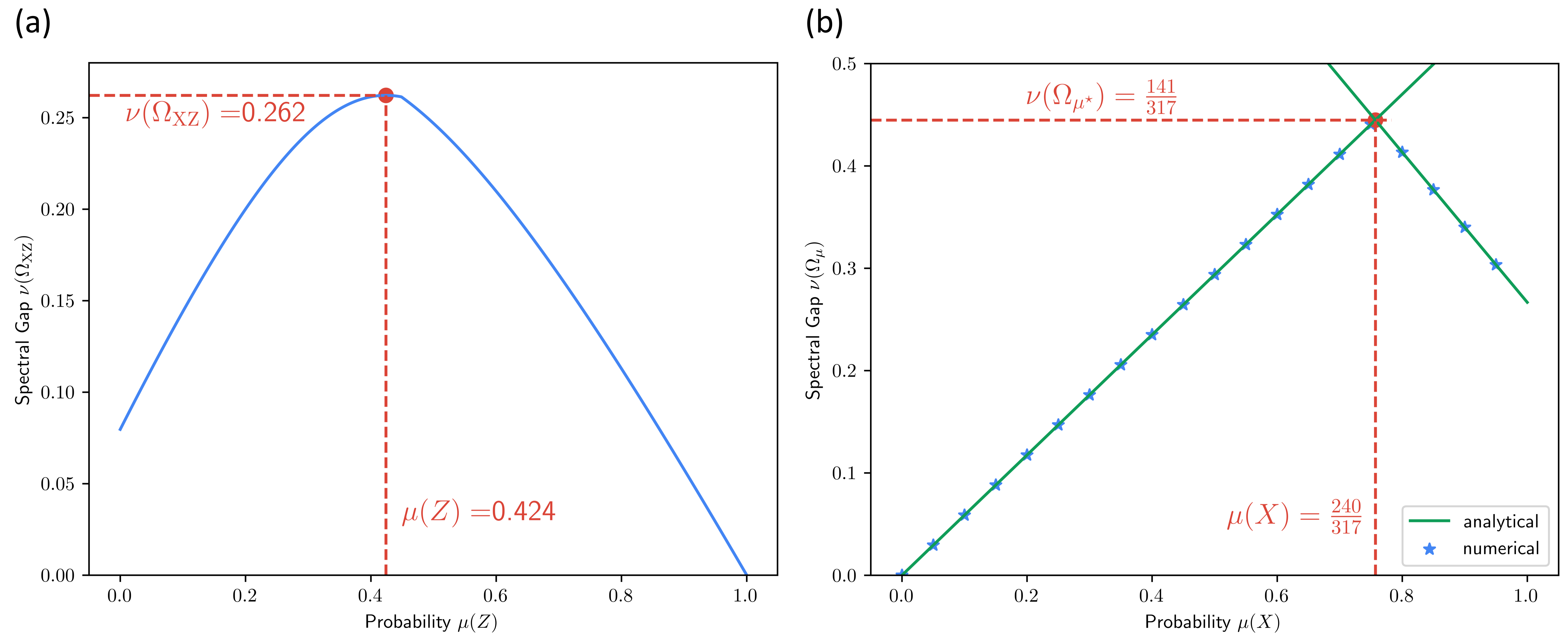
Figure 1: (a) Numerical result of the XZ strategy. The probability $\mu(Z)$ is sampled from $0$ to $1$ with a step size of $0.001$, and the spectral gaps are computed. The maximal spectral gap is achieved when $\mu(Z)\approx 0.424$. (b) Analytical and numerical results of the rotation strategy. The two green lines represent the functions $\frac{47}{80}\mu(X)$ and $1-\frac{11}{15}\mu(X)$, respectively. The blue stars indicate the numerical results of the rotation strategy, where $\mu(X)$ is sampled from $0$ to $1$ with a step size of $0.05$. The maximal spectral gap is achieved when $\mu(X)=\frac{240}{317}$.

IV.3 Rotation strategy

The XZ strategy, while effective, lacks an analytical solution and exhibits a sample complexity approximately four times that of the globally optimal strategy. To address these limitations, we introduce the rotation strategy, utilizing ten test operators. This strategy, for which we derive an analytical performance, achieves a sample complexity approximately twice that of the globally optimal strategy.

The strategy.

In each round, we select a measurement $P\in\{X,Z\}$ according to a probability distribution $\mu(P)$, which will be optimized later. If the $Z$ measurement is chosen, we perform the test operator $M_{Z}$. Otherwise, we apply $U_{1}$, $U_{2}$ or $\emptyset$ (no unitary at all) uniformly at random, followed by choosing one qubit uniformly at random to carry out the test project $M_{X,i}$. Mathematically, this test operator can be written as

$$\widehat{M}_{X}\mathrel{\mathop{\mathchar 58\relax}}=\frac{1}{3}\sum_{i=1}^{3}M_{X,i}^{\prime},$$ (35)

where

$$M^{\prime}_{X,i}\mathrel{\mathop{\mathchar 58\relax}}=\frac{1}{3}(M_{X,i}+U_{1}^{\dagger}M_{X,i}U_{1}+U_{2}^{\dagger}M_{X,i}U_{2}).$$ (36)

Therefore, the verification operator for this strategy is given by

$$\Omega_{\mu}\mathrel{\mathop{\mathchar 58\relax}}=\mu(Z)M_{Z}+\mu(X)\widehat{M}_{X},$$ (37)

where $\mu$ is a probability distribution satisfying $\sum_{P}\mu(P)=1$. The whole procedure is illustrated in Fig. 2.

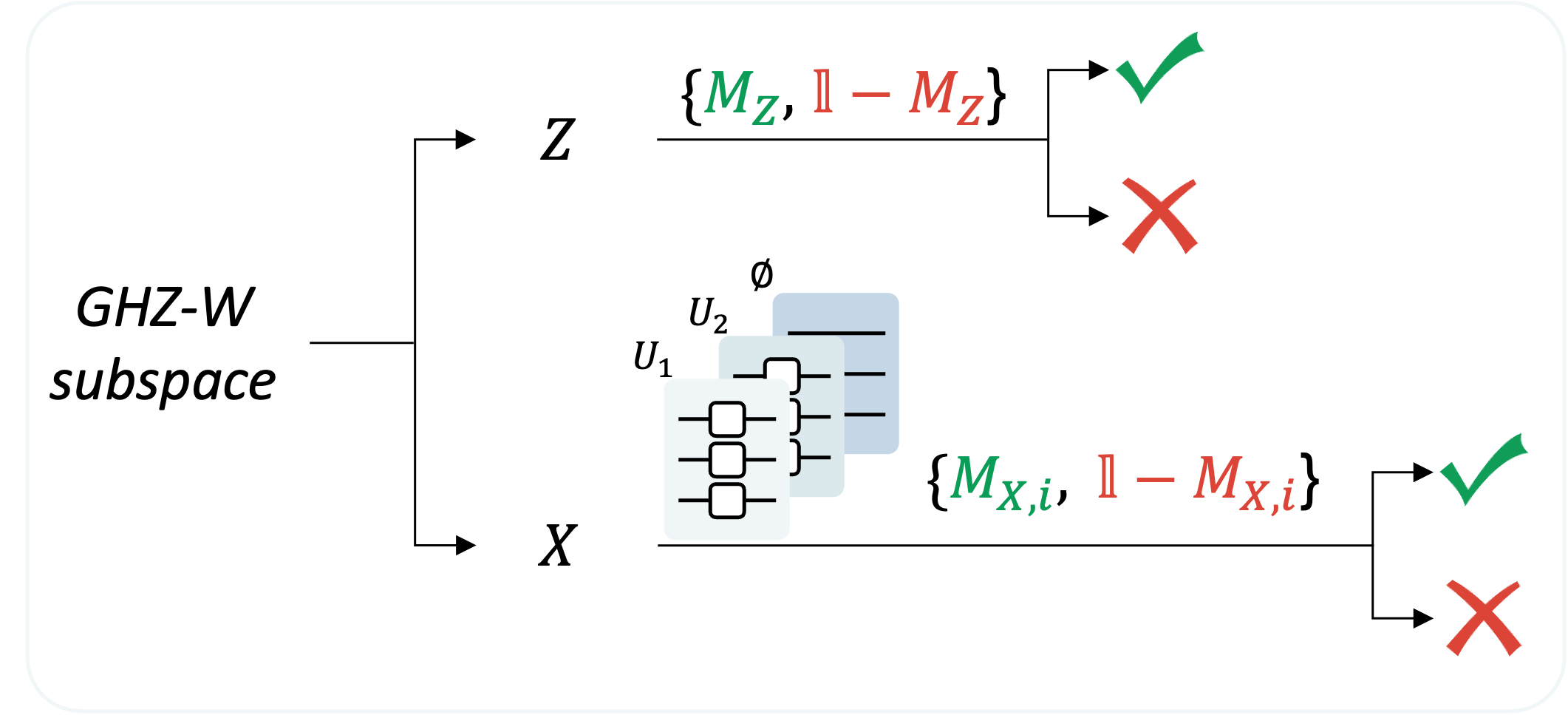
Figure 2: The one-way adaptive verification strategy for GHZ-W subspace. We first randomly select $P\in\{X,Z\}$ according to a predefined probability distribution $\mu$. (1) If $P=Z$, we perform the test operator $M_{Z}$. (2) If $P=X$, we apply a unitary gate randomly chosen from the set $\{U_{1},U_{2},\emptyset\}$, where $\emptyset$ denotes applying no gate. Then, we perform the test operator $M_{X,i}$ starting with an $X$ measurement on the $i$-th qubit. Based on its measurement result, we proceed with a two-qubit verification strategy on the remaining qubits.

Performance analysis.

Obviously, the choice of $\mu(P)$ influences the performance of the strategy. Fortunately, the optimal probability distribution can be determined analytically, as shown in the following lemma.

Lemma 4.

The strategy operator defined in Eq. (37), achieves the largest spectral gap of $141/317\approx 0.445$ when $\mu^{\star}(X)=240/317\approx 0.757$.

Proof.

The analysis of the spectral gap relies on the invariant properties of the subspace $\mathcal{V}_{3}$. Suppose $M$ is a test operator for the subspace $\mathcal{V}_{3}$. Define

$$M^{\prime} \mathrel{\mathop{\mathchar 58\relax}}=\frac{1}{3}\left(M+U_{1}^{\dagger}MU_{1}+U_{2}^{\dagger}MU_{2}\right).$$ (38)

With the fact that $\mathcal{V}_{3}$ is invariant under $U_{i}$, each term $U_{i}MU_{i}^{\dagger}$ is also a valid test operator. Then, incorporating qubit permutations, the averaged operator of $M$ can be defined as

$$\overline{M}\mathrel{\mathop{\mathchar 58\relax}}=\frac{1}{6}\sum_{\pi\in\mathbb{S}_{3}}V_{\pi}M^{\prime}V_{\pi}^{\dagger}=\left[\begin{matrix}a&0&0&0&0&0&0&b\\ 0&d&e&0&e&0&0&0\\ 0&e&d&0&e&0&0&0\\ 0&0&0&f&0&g&g&0\\ 0&e&e&0&d&0&0&0\\ 0&0&0&g&0&f&g&0\\ 0&0&0&g&0&g&f&0\\ b&0&0&0&0&0&0&c\end{matrix}\right],$$ (39)

where $a,b,c,d,e,f,g$ are coefficients. As $M$ is a test operator, the states $|{{\rm GHZ}}\rangle$ and $|{{\rm W}}\rangle$ are eigenstates of $\overline{M}$, i.e.,

$$\begin{cases}\overline{M}|{\rm GHZ}\rangle=|{\rm GHZ}\rangle\\ \overline{M}|{\rm W}\rangle=|{\rm W}\rangle\end{cases}\quad\Rightarrow\quad\begin{cases}d=1-2e\\ b=1-a\\ c=a\end{cases}.$$ (40)

Therefore, $\overline{M}$ reduces to the form

$$\overline{M}=\left[\begin{matrix}a&0&0&0&0&0&0&1-a\\ 0&1-2e&e&0&e&0&0&0\\ 0&e&1-2e&0&e&0&0&0\\ 0&0&0&f&0&g&g&0\\ 0&e&e&0&1-2e&0&0&0\\ 0&0&0&g&0&f&g&0\\ 0&0&0&g&0&g&f&0\\ 1-a&0&0&0&0&0&0&a\end{matrix}\right].$$ (41)

In addition to $|{{\rm GHZ}}\rangle$ and $|{{\rm W}}\rangle$, the other eigenstates and eigenvalues are:

$$|{v_{1}}\rangle =\frac{1}{\sqrt{2}}(|{000}\rangle-|{111}\rangle),\quad\lambda_{1}=2a-1,$$ (42)

$$|{v_{2}}\rangle =\frac{1}{\sqrt{2}}(|{001}\rangle-|{010}\rangle),\quad\lambda_{2}=1-3e,$$ (43)

$$|{v_{3}}\rangle =\frac{1}{\sqrt{2}}(|{001}\rangle-|{100}\rangle),\quad\lambda_{3}=1-3e,$$ (44)

$$|{v_{4}}\rangle =\frac{1}{\sqrt{2}}(|{011}\rangle-|{101}\rangle),\quad\lambda_{4}=f-g,$$ (45)

$$|{v_{5}}\rangle =\frac{1}{\sqrt{2}}(|{011}\rangle-|{110}\rangle),\quad\lambda_{5}=f-g,$$ (46)

$$|{v_{6}}\rangle =\frac{1}{\sqrt{3}}(|{011}\rangle+|{101}\rangle+|{110}\rangle)\quad\lambda_{6}=f+2g.$$ (47)

Obviously, the spectral gap of $\overline{M}$ is given by

$$\nu(\overline{M}) =1-\max\{2a-1,1-3e,f-g,f+2g\}.$$ (48)

Now consider the verification operator $\Omega_{\mu}$, defined in Eq. (37). With the definitions of $M_{Z}$ and $\widehat{M}_{X}$, we have

$$M_{Z} =\overline{M}_{Z},$$ (49)

$$\widehat{M}_{X} =\overline{M}_{X}.$$ (50)

Therefore, the spectral gap of $\Omega_{\mu}$ is given by

$$\nu(\Omega_{\mu}) =1-\max\left\{1-\frac{13}{20}\mu(X),1-\frac{47}{80}\mu(X),\frac{131}{240}\mu(X),\frac{11}{15}\mu(X)\right\}$$ (51)

$$=\min\left\{\frac{47}{80}\mu(X),1-\frac{11}{15}\mu(X)\right\}.$$ (52)

Thus, when $\mu^{\star}(X)=240/317$, the spectral gap reaches its maximum value:

$$\nu(\Omega_{\mu^{\star}})=\frac{141}{317}.$$ (53)

∎

We also compare our analytical results with the numerical results, as shown in Fig. 1(b). We sample $\mu(X)$ from $0$ to $1$ with a step size of $0.05$ and find that the results are consistent. Therefore, to achieve a confidence level of $1-\delta$, the required number of state copies is given by

$$N(\Omega_{\mu^{\star}})=\frac{317}{141}\times\frac{1}{\epsilon}\ln\frac{1}{\delta}\approx 2.248\times\frac{1}{\epsilon}\ln\frac{1}{\delta}.$$ (54)

IV.4 Comparisons

As mentioned previously, to achieve a confidence level of $1-\delta$, the globally optimal verification requires only $\ln(1/\delta)/\epsilon$ state copies, but it involves entangled measurements. In this section, we proposed two verification strategies based on one-way adaptive measurements: the XZ strategy and the rotation strategy. The XZ strategy requires a total of four test operators, while the rotation strategy requires ten test operators. However, the rotation strategy requires approximately $2.248\ln(1/\delta)/\epsilon$ state copies, which is fewer than the XZ strategy. In Fig. 3, we compare the efficiency of these strategies. We set $\delta=0.001$ and adjust $\epsilon$ from $0.001$ to $0.1$. Each line represents the minimum number of state copies required to achieve a confidence level of $1-\delta$. The globally optimal verification strategy is the most efficient, with the rotation strategy surpassing the XZ strategy in efficiency. However, executing the globally optimal strategy is experimentally challenging. Practically, the same confidence level is attainable with a few local measurement settings, requiring about double the state copies compared to the global approach.

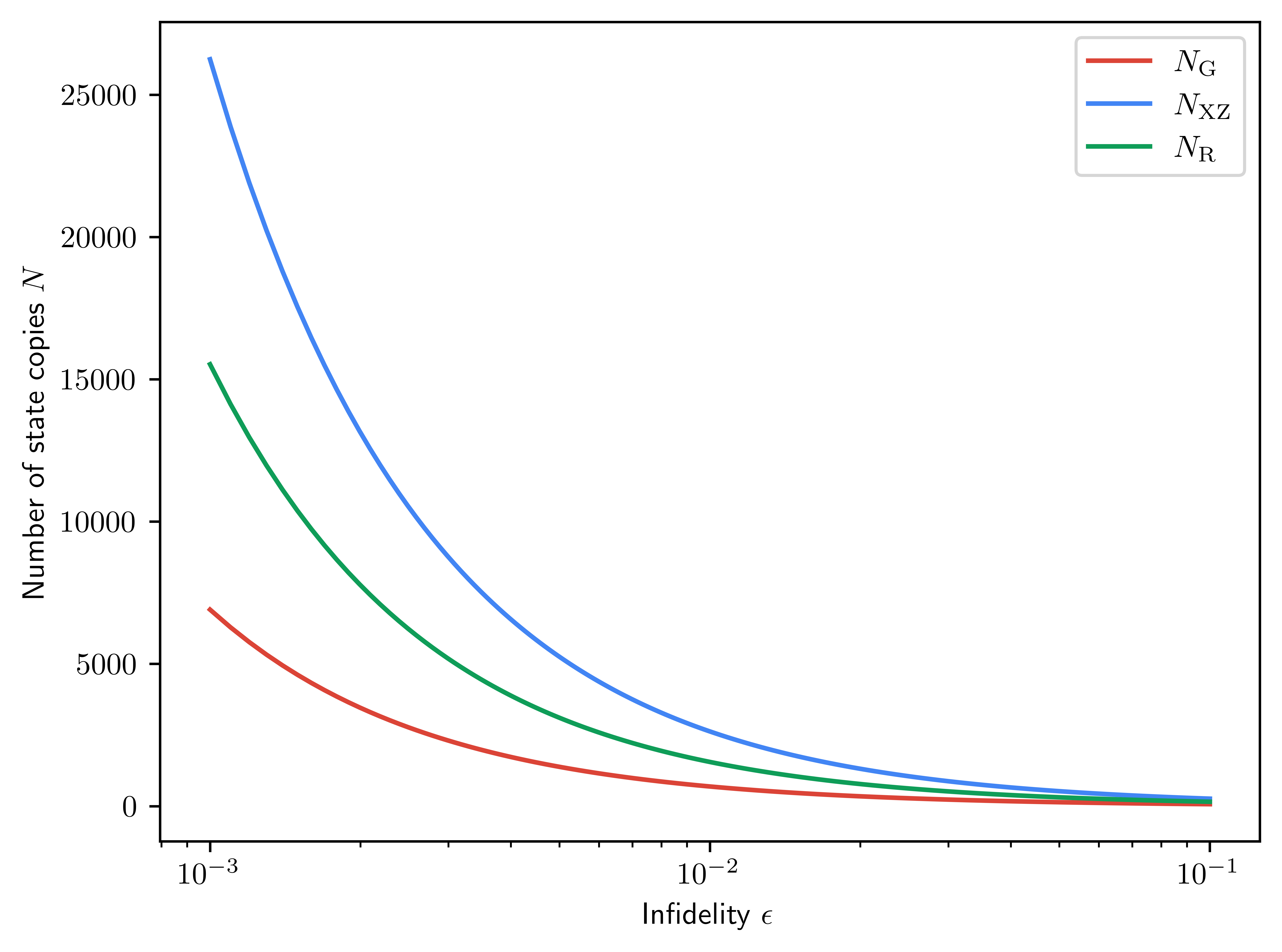
Figure 3: Comparison of the total number of state copies required to verify the three-qubit GHZ-W subspace for different strategies as a function of the infidelity $\epsilon$, where $\delta=0.001$. Here, $N_{\rm G}$ is the sample complexity of the globally optimal strategy given in Eq. (5), $N_{\rm XZ}$ is the sample complexity of the XZ strategy given in Eq. (34), and $N_{\rm R}$ is the sample complexity of the rotation strategy given in Eq. (54).

V Conclusions

In this work, we investigated the task of verifying the three-qubit GHZ-W genuinely entangled subspace using adaptive local measurements. By exploiting the local symmetry properties of the GHZ-W subspace, we first designed ten test operators and then constructed two efficient verification strategies: the XZ strategy and the rotation strategy. The XZ strategy, employing four test operators, requires approximately $3.817/\epsilon\ln(1/\delta)$ state copies to achieve a confidence level of $1-\delta$. In contrast, the rotation strategy, utilizing all ten test operators, achieves the same confidence level with a reduced sample complexity of $2.248/\epsilon\ln(1/\delta)$. Notably, the sample complexity of the rotation strategy is only approximately twice that of the globally optimal verification strategy, demonstrating its high efficiency. Along the way, we comprehensively analyzed the two-dimensional two-qubit subspaces, classifying them into three distinct types: unverifiable, verifiable, and perfectly verifiable subspaces. Interestingly, we demonstrated the existence of two-qubit entangled subspaces that are inherently unverifiable with local measurements, highlighting fundamental limitations in local entanglement verification.

Our findings raise several important open questions. A primary challenge lies in formulating and rigorously proving optimal verification strategies with local measurements for arbitrary subspaces. Moreover, extending our approach to larger GHZ-W subspaces and other entangled subspaces remains an open area of research.

References

- Horodecki et al. [2009] R. Horodecki, P. Horodecki, M. Horodecki, and K. Horodecki, Quantum entanglement, Reviews of Modern Physics 81, 865 (2009).
- Horodecki et al. [2024] P. Horodecki, Ł. Rudnicki, and K. Życzkowski, Multipartite entanglement (2024), arXiv:2409.04566 .
- Chen et al. [2024a] Y.-A. Chen, X. Liu, C. Zhu, L. Zhang, J. Liu, and X. Wang, Quantum entanglement allocation through a central hub (2024a), arXiv:2409.08173 .
- Dür et al. [2000] W. Dür, G. Vidal, and J. I. Cirac, Three qubits can be entangled in two inequivalent ways, Physical Review A 62, 062314 (2000).
- Acín et al. [2001] A. Acín, D. Bruß, M. Lewenstein, and A. Sanpera, Classification of mixed three-qubit states, Physical Review Letters 87, 040401 (2001).
- Walther et al. [2005] P. Walther, K. J. Resch, and A. Zeilinger, Local conversion of greenberger-horne-zeilinger states to approximate w states, Physical Review Letters 94, 240501 (2005).
- Alsina and Razavi [2021] D. Alsina and M. Razavi, Absolutely maximally entangled states, quantum-maximum-distance-separable codes, and quantum repeaters, Physical Review A 103, 022402 (2021).
- Gour and Wallach [2007] G. Gour and N. R. Wallach, Entanglement of subspaces and error-correcting codes, Physical Review A 76, 042309 (2007).
- Huber and Grassl [2020] F. Huber and M. Grassl, Quantum codes of maximal distance and highly entangled subspaces, Quantum 4, 284 (2020).
- Raissi et al. [2018] Z. Raissi, C. Gogolin, A. Riera, and A. Acín, Optimal quantum error correcting codes from absolutely maximally entangled states, Journal of Physics A: Mathematical and Theoretical 51, 075301 (2018).
- Shenoy and Srikanth [2019] A. H. Shenoy and R. Srikanth, Maximally nonlocal subspaces, Journal of Physics A: Mathematical and Theoretical 52, 095302 (2019).
- Demianowicz [2022] M. Demianowicz, Universal construction of genuinely entangled subspaces of any size, Quantum 6, 854 (2022), arxiv:2111.10193 [quant-ph] .
- Baccari et al. [2020] F. Baccari, R. Augusiak, I. Šupić, and A. Acín, Device-independent certification of genuinely entangled subspaces, Physical Review Letters 125, 260507 (2020).
- Makuta and Augusiak [2021] O. Makuta and R. Augusiak, Self-testing maximally-dimensional genuinely entangled subspaces within the stabilizer formalism, New Journal of Physics 23, 043042 (2021).
- Demianowicz and Augusiak [2018] M. Demianowicz and R. Augusiak, From unextendible product bases to genuinely entangled subspaces, Physical Review A 98, 012313 (2018).
- Demianowicz et al. [2021] M. Demianowicz, G. Rajchel-Mieldzioć, and R. Augusiak, Simple sufficient condition for subspace to be completely or genuinely entangled, New Journal of Physics 23, 103016 (2021).
- Demianowicz and Augusiak [2019] M. Demianowicz and R. Augusiak, Entanglement of genuinely entangled subspaces and states: Exact, approximate, and numerical results, Physical Review A 100, 062318 (2019).
- Park et al. [2008] D. Park, S. Tamaryan, and J.-W. Son, Role of three-qubit mixed-states entanglement in teleportation scheme (2008), arXiv:0808.4045 .
- Chakrabarty [2010] I. Chakrabarty, Teleportation via a mixture of a two qubit subsystem of a n-qubit w and ghz state, The European Physical Journal D 57, 265 (2010), arXiv:0901.4473 [quant-ph] .
- Lohmayer et al. [2006] R. Lohmayer, A. Osterloh, J. Siewert, and A. Uhlmann, Entangled three-qubit states without concurrence and three-tangle, Physical Review Letters 97, 260502 (2006).
- Wang and Shi [2015] X. Wang and X. Shi, Classifying entanglement in the superposition of greenberger-horne-zeilinger and w states, Physical Review A 92, 042318 (2015).
- Xie et al. [2023] S. Xie, D. Younis, and J. H. Eberly, Evidence for unexpected robustness of multipartite entanglement against sudden death from spontaneous emission, Physical Review Research 5, L032015 (2023).
- Faujdar et al. [2023] J. Faujdar, H. Kaur, P. Singh, A. Kumar, and S. Adhikari, Nonlocality and efficiency of three-qubit partially entangled states, Quantum Studies: Mathematics and Foundations 10, 27 (2023).
- Zheng et al. [2020] R.-H. Zheng, Y.-H. Kang, D. Ran, Z.-C. Shi, and Y. Xia, Deterministic interconversions between the greenberger-horne-zeilinger states and the w states by invariant-based pulse design, Physical Review A 101, 012345 (2020).
- Häffner et al. [2005] H. Häffner, W. Hänsel, C. F. Roos, J. Benhelm, D. Chek-al kar, M. Chwalla, T. Körber, U. D. Rapol, M. Riebe, P. O. Schmidt, C. Becher, O. Gühne, W. Dür, and R. Blatt, Scalable multiparticle entanglement of trapped ions, Nature 438, 643–646 (2005).
- Xue et al. [2022] S. Xue, Y. Wang, J. Zhan, Y. Wang, R. Zeng, J. Ding, W. Shi, Y. Liu, Y. Liu, A. Huang, G. Huang, C. Yu, D. Wang, X. Fu, X. Qiang, P. Xu, M. Deng, X. Yang, and J. Wu, Variational entanglement-assisted quantum process tomography with arbitrary ancillary qubits, Phys. Rev. Lett. 129, 133601 (2022).
- Eisert et al. [2020] J. Eisert, D. Hangleiter, N. Walk, I. Roth, D. Markham, R. Parekh, U. Chabaud, and E. Kashefi, Quantum certification and benchmarking, Nature Reviews Physics 2, 382 (2020).
- Kliesch and Roth [2021] M. Kliesch and I. Roth, Theory of quantum system certification, PRX Quantum 2, 010201 (2021).
- Huang et al. [2020] H.-Y. Huang, R. Kueng, and J. Preskill, Predicting many properties of a quantum system from very few measurements, Nature Physics 16, 1050 (2020).
- Elben et al. [2020] A. Elben, B. Vermersch, R. van Bijnen, C. Kokail, T. Brydges, C. Maier, M. Joshi, R. Blatt, C. F. Roos, and P. Zoller, Cross-platform verification of intermediate scale quantum devices, Physical Review Letters 124, 010504 (2020), arxiv:1909.01282 [cond-mat, physics:quant-ph] .
- Elben et al. [2023] A. Elben, S. T. Flammia, H.-Y. Huang, R. Kueng, J. Preskill, B. Vermersch, and P. Zoller, The randomized measurement toolbox, Nature Reviews Physics 5, 9 (2023).
- Zheng et al. [2024a] C. Zheng, X. Yu, and K. Wang, Cross-platform comparison of arbitrary quantum processes, npj Quantum Information 10, 1 (2024a).
- Pallister et al. [2018] S. Pallister, N. Linden, and A. Montanaro, Optimal verification of entangled states with local measurements, Physical Review Letters 120, 170502 (2018).
- Wang and Hayashi [2019] K. Wang and M. Hayashi, Optimal verification of two-qubit pure states, Physical Review A 100, 032315 (2019).
- Yu et al. [2022] X.-D. Yu, J. Shang, and O. Gühne, Statistical methods for quantum state verification and fidelity estimation, Advanced Quantum Technologies 5, 2100126 (2022).
- Li et al. [2020] Z. Li, Y.-G. Han, and H. Zhu, Optimal verification of greenberger-horne-zeilinger states, Physical Review Applied 13, 054002 (2020).
- Dangniam et al. [2020] N. Dangniam, Y.-G. Han, and H. Zhu, Optimal verification of stabilizer states, Physical Review Research 2, 043323 (2020).
- Chen et al. [2024b] S. Chen, W. Xie, P. Xu, and K. Wang, Quantum memory assisted entangled state verification with local measurements (2024b), arXiv:2312.11066 [quant-ph] .
- Li et al. [2021] Z. Li, Y.-G. Han, H.-F. Sun, J. Shang, and H. Zhu, Verification of phased dicke states, Physical Review A 103, 022601 (2021).
- Jiang et al. [2020] X. Jiang, K. Wang, K. Qian, Z. Chen, Z. Chen, L. Lu, L. Xia, F. Song, S. Zhu, and X. Ma, Towards the standardization of quantum state verification using optimal strategies, npj Quantum Information 6, 90 (2020).
- Zhang et al. [2020] W.-H. Zhang, C. Zhang, Z. Chen, X.-X. Peng, X.-Y. Xu, P. Yin, S. Yu, X.-J. Ye, Y.-J. Han, J.-S. Xu, G. Chen, C.-F. Li, and G.-C. Guo, Experimental optimal verification of entangled states using local measurements, Physical Review Letters 125, 030506 (2020).
- Xia et al. [2022] L. Xia, L. Lu, K. Wang, X. Jiang, S. Zhu, and X. Ma, Experimental optimal verification of three-dimensional entanglement on a silicon chip, New Journal of Physics 24, 095002 (2022).
- Chitambar et al. [2014] E. Chitambar, D. Leung, L. Mančinska, M. Ozols, and A. Winter, Everything You Always Wanted to Know About LOCC (But Were Afraid to Ask), Communications in Mathematical Physics 328, 303–326 (2014).
- Zheng et al. [2024b] C. Zheng, X. Yu, Z. Zhang, P. Xu, and K. Wang, Efficient verification of stabilizer code subspaces with local measurements (2024b), arXiv:2409.19699 .
- Chen et al. [2024c] J. Chen, P. Zeng, Q. Zhao, X. Ma, and Y. Zhou, Quantum subspace verification for error correction codes (2024c), arXiv:2410.12551 .
- Demianowicz and Augusiak [2020] M. Demianowicz and R. Augusiak, An approach to constructing genuinely entangled subspaces of maximal dimension, Quantum Information Processing 19, 199 (2020).
- Parthasarathy [2004] K. R. Parthasarathy, On the maximal dimension of a completely entangled subspace for finite level quantum systems, Proceedings Mathematical Sciences 114, 365 (2004).
- Duan et al. [2009] R. Duan, Y. Feng, Y. Xin, and M. Ying, Distinguishability of quantum states by separable operations, IEEE Transactions on Information Theory 55, 1320 (2009).
- Wootters [1998] W. K. Wootters, Entanglement of formation of an arbitrary state of two qubits, Physical Review Letters 80, 2245 (1998).