On the approximation of spatial convolutions
by PDE systems

Abstract.

This paper considers the approximation problem for the spatial convolution with a given integral kernel. The approximation to the spatial convolution by PDE systems has been proposed to eliminate the analytical difficulties caused by the integrals for the one-dimensional space. In this paper we establish a PDE system approximation for the spatial convolutions in higher spatial dimensions. We derive an approximation function for given arbitrary radial integral kernels by linear sums of the Green functions. In the proof of this methodology we introduce an appropriate integral transformation to show the completeness of the basis constructed by the Green functions. From this theory, it is possible to approximate the nonlocal operator of the convolution type with any radial integral kernels by the linear sum of the solutions to the PDE system. Finally, numerical examples for the approximation are demonstrated using this method.

1. Introduction

In this paper, we consider the approximation problem for the convolution

$$(K*u)(t,x):=\int_{{\mathbb{R}}^{n}}K(x-y)u(t,y)dy=\int_{{\mathbb{R}}^{n}}K(y)u(t,x-y)dy$$

with respect to the spatial variable $x\in{\mathbb{R}}^{n}$, where the integral kernel $K:{\mathbb{R}}^{n}\to{\mathbb{R}}$ is a radial function in $L^{1}({\mathbb{R}}^{n})$ and $u(t):{\mathbb{R}}^{n}\to{\mathbb{R}}$ is a measurable function for any time variable $t\geq 0$. Evolution equations with the convolution are appeared as mathematical models in various fields such as material science [5], neuroscience [3], cell biology [13, 19, 24] and ecology [17, 23]. Such mathematical models are applied for the theoretical understanding of interface phenomena, pattern formation problems and so on. In the studies of pattern formation problems, it is known that various complex patterns are generated depending on the shapes of integral kernel in numerical simulations of such models [13, 19]. For understanding of mathematical structure of solutions to evolution equations with spatial convolutions, many analytical methods have been proposed (e.g. [4, 6, 7, 9, 11, 12]). The difficulties of mathematical analysis include that the convolution yields a limited understanding of local properties of the solution, and that it is computationally expensive in numerical simulations. To overcome such difficulties, methodologies that approximate the convolution by derivatives of the function have been developed in recent years. One of the proposed methods is an approximation using the Taylor expansion of $u(t,x)$ [1, 6, 21, 24]. The idea of the method is come from the fact that the convolution can be formally expanded by

$$(K*u)(t,x) = \left(\int_{{\mathbb{R}}^{n}}K(y)dy\right)u(t,x)-\int_{{\mathbb{R}}^{n}}\left\langle\right.y,\nabla_{x}u(t,x)\left.\right\rangle K(y)dy$$

$$\quad\quad+\dfrac{1}{2}\int_{{\mathbb{R}}^{n}}\left\langle\right.y,\nabla^{2}_{x}u(t,x)y\left.\right\rangle K(y)dy+\cdots.$$

Thus, the convolution is approximately expressed by a differential operator with coefficients which has the information of the integral kernel. The validity of the method has been discussed by [1, 6] when $n=1$. It has been shown that it is applicable in limited situations, such as when the range of the support of the integral kernel is sufficiently narrow.

On the other hand, it is also a well used methodology to rewrite the convolution into a PDE system by giving the integral kernel as a linear sum of the Green functions [2, 14, 15, 20]. In particular, the Green function $k(x;d)$ with a constant $d>0$ which is given by the solution of

$$d\Delta k(x)-k(x)+\delta(x)=0\quad(x\in{\mathbb{R}}^{n})$$

is often used, where $\delta(x)$ is the Dirac delta function. Here, $k(x;d)$ is represented as

$$k(x;d) := \left(\dfrac{1}{d}\right)^{n/2}G\left(\dfrac{|x|}{\sqrt{d}}\right),$$

(1.1) $$G(|x|) := \dfrac{1}{(2\pi)^{n/2}}\left(\dfrac{1}{|x|}\right)^{n/2-1}M_{n/2-1}\left(|x|\right),$$

where $M_{\nu}(r)$ is the modified Bessel function of the second kind with the order $\nu$ defined as

$$M_{\nu}(r):=\int^{+\infty}_{0}e^{-r\cosh s}\cosh(\nu s)ds.$$

The green function is represented by

$$k(x;d)=\dfrac{1}{2\sqrt{d}}e^{-|x|/\sqrt{d}},$$

when $n=1$, and

$$k(x;d)=\dfrac{1}{2d\pi}M_{0}\left(\dfrac{|x|}{\sqrt{d}}\right)$$

when $n=2$. When we give the integral kernel as

$$K(x)=\displaystyle\sum^{N}_{j=1}\alpha_{j}k(x;d_{j})$$

with $N\in{\mathbb{N}}$, constants $\{\alpha_{j}\}_{1\leq j\leq N}$ and positive constants $\{d_{j}\}_{1\leq j\leq N}$, the convolution is represented as

$$(K*u)(t,x)=\displaystyle\sum^{N}_{j=1}\alpha_{j}w_{j}(t,x),$$

$$d_{j}\Delta w_{j}(t,x)-w_{j}(t,x)+u(t,x)=0\quad(j=1,2,\ldots,N).$$

Namely, the convolution is expressed as the linear sum of the solution to the PDE system. This method can only handle integral kernels that can be expressed as linear sums of the Green functions. However, it is useful in mathematical analysis because PDE systems can be derived without the need for any approximations.

For general integral kernels, when the integral kernel can be approximated by a linear sum of the Green functions under $L^{p}$ norm with $p\in[1,+\infty]$, the Young inequality allows for the error estimate of the approximation of the convolution. It is therefore sufficient to consider a class of integral kernels that can be approximated by a linear sum of the Green functions for a given norm. When $n=1$, the approximations of integral kernels by the Green functions under $L^{2}$-norm and $L^{\infty}$-norm have been reported [22, 25, 26]. In this case, the method of the approximation theory of polynomials is effective for the approximation of kernels since $k(x;d)$ is represented by an exponential function. In the light of considering phenomena such as neuroscience [10, 16], pattern formation problems [13, 19], and cell motility [8, 27], it is more important to develop the method in the 2-dimensional and 3-dimensional spatial cases.

Based on above, this paper considers an approximation to radial integral kernels by linear sums of the Green functions for the purpose of approximating the convolution with the PDE system. The paper is organized as follows. In Section 2, we introduce main results for the approximation of radial integral kernels. The proof is given in Section 3. We then give a numerical example in Section 4 and concluding remarks in Section 5.

2. Approximation theorem

Here we state our main result on the approximation of integral kernels. Let $\{d_{j}\}_{j\in{\mathbb{N}}}$ be positive constants. For sake of simplicity, we set

$$k_{j}(x):=k(x;d_{j}).$$

Then, we obtain the following main theorem.

Theorem 2.1.

Let $m$ be a non-negative integer and $\{d_{j}\}_{j\in{\mathbb{N}}}$ be a sequence of distinct positive constants which has a positive accumulation point. Assume that $K\in H^{m}({\mathbb{R}}^{n})$ is a radial function. Then, for any $\epsilon>0$, there exist $N=N(m,n,\epsilon)\in{\mathbb{N}}$ that is greater than $(2m+n-1)/4$ and constants $\{\alpha_{j}^{N}\}_{1\leq j\leq N}$ such that

$$\displaystyle\sum^{N}_{j=1}\alpha_{j}^{N}k_{j}\in H^{m}({\mathbb{R}}^{n})$$

and

$$\left\|K-\displaystyle\sum^{N}_{j=1}\alpha_{j}^{N}k_{j}\right\|_{H^{m}}<\epsilon$$

hold.

From the definition of the Green function, $k(\cdot;d)\in L^{2}({\mathbb{R}}^{n})$ holds only if $n\leq 3$. It is a property that follows from the singularity at the origin of the modified Bessel function of the second kind. However, we can resolve the singularity by considering a linear sum of the Green functions, which allows us to consider an approximation for the functions in $H^{m}({\mathbb{R}}^{n})$.

The approach of the proof is to show completeness for a linear span of the Green functions based on the theory of the orthogonal basis. Since we use the identity theorem for analytic functions when considering completeness, we include an assumption about the accumulation point for $\{d_{j}\}_{j\in{\mathbb{N}}}$. The proof is given in Section 3.

We mention approximations in other norms to the one used in the main result. For a nonnegative integer $l$ with $m>n/2+l$, it is known that

$$H^{m}({\mathbb{R}}^{n})\subset C^{l}({\mathbb{R}}^{n})$$

from the the Morrey inequality. Thus, we find a $C^{l}$-approximation when $m>n/2+l$ and $K\in H^{m}({\mathbb{R}}^{n})$. Moreover, for any $s\in{\mathbb{R}}$, we obtain a $H^{s}$-approximation of a kernel belonging to $H^{m}({\mathbb{R}}^{n})$ with $m>s$. Especially, for $p>2$, we also obtain a $L^{p}$-approximation from the Sobolev embedding theory. The case $p\in[1,2)$ has not yet been derived by this result and a part of it is still an open problem.

For the convolution, the Young inequality yields the following result.

Corollary 2.2.

Let $s\in[0,n/2)$ and $m\in{\mathbb{N}}\cup\{0\}$ satisfy $m\geq s$. When $K\in H^{m}({\mathbb{R}}^{n})$, for any $\epsilon>0$, there exist $N=N(m,n,\epsilon)\in{\mathbb{N}}$ and constants $\{\alpha_{j}^{N}\}_{1\leq j\leq N}$ such that

$$\left\|K*f-\displaystyle\sum^{N}_{j=1}\alpha_{j}^{N}k_{j}*f\right\|_{L^{r}}\leq\epsilon\|f\|_{L^{q}}$$

holds for $q,r\in[1,+\infty]$ with $\dfrac{1}{q}=\dfrac{1}{r}+\dfrac{n+2s}{2n}$ and $f\in L^{q}({\mathbb{R}}^{n})$.

Proof.

Let $s\in[0,n/2)$. Then, there is $C=C(s,n)>0$ such that

$$\|K\|_{L^{2n/(n-2s)}}\leq C\|K\|_{H^{s}}\leq C\|K\|_{H^{m}}$$

holds from the Sobolev embedding theory. From Theorem 2.1, there exist $N=N(m,n,\epsilon)\in{\mathbb{N}}$ and constants $\{\alpha_{j}^{N}\}_{1\leq j\leq N}$ such that

$$\left\|K-\displaystyle\sum^{N}_{j=1}\alpha_{j}^{N}k_{j}\right\|_{H^{m}}\leq\dfrac{\epsilon}{C}.$$

Therefore, we obtain

$$\left\|K*f-\displaystyle\sum^{N}_{j=1}\alpha_{j}^{N}k_{j}*f\right\|_{L^{r}} \leq \left\|K-\displaystyle\sum^{N}_{j=1}\alpha_{j}^{N}k_{j}\right\|_{L^{2n/(n-2s)}}\|f\|_{L^{q}}$$

$$\leq C\left\|K-\displaystyle\sum^{N}_{j=1}\alpha_{j}^{N}k_{j}\right\|_{H^{m}}\|f\|_{L^{q}}\leq\epsilon\|f\|_{q}.$$

∎

3. Completeness of a linear span of the Green functions

In this section we give the proof of Theorem 2.1. Through this section we set $\{d_{j}\}_{j\in{\mathbb{N}}}$ as distinct positive constants.

3.1. Properties of the Green function

We introduce some properties of the Green function. The Fourier transform of $G(|x|)$ defined by (1.1) is computed as

$$\hat{G}(\xi)=\mathcal{F}_{n}[G](\xi) := \int_{{\mathbb{R}}^{n}}e^{-ix\cdot\xi}G(|x|)dx$$

$$= (2\pi)^{n/2}\left(\dfrac{1}{|\xi|}\right)^{n/2-1}\int^{+\infty}_{0}J_{n/2-1}(|\xi|r)G(r)r^{n/2}dr$$

$$= \left(\dfrac{1}{|\xi|}\right)^{n/2-1}\int^{+\infty}_{0}rJ_{n/2-1}(|\xi|r)M_{n/2-1}\left(r\right)dr$$

for $|\xi|>0$, where $J_{n/2-1}(r)$ is the Bessel function with the order $n/2-1$. Since it is known from [29, §13.45] that

$$\int^{+\infty}_{0}rJ_{n/2-1}(|\xi|r)M_{n/2-1}\left(r\right)dr=|\xi|^{n/2-1}{}_{2}F_{1}\left(\dfrac{n}{2},1;\dfrac{n}{2};-|\xi|^{2}\right)=\dfrac{|\xi|^{n/2-1}}{1+|\xi|^{2}},$$

we have $\hat{G}(\xi)=1/(1+|\xi|^{2})$. Here, ${}_{2}F_{1}(a,b;c;z)$ is the hypergeometric function.

It is easy to see that $G(|x|)$ is positive for $|x|>0$. By using the integral formula

$$\int^{+\infty}_{0}r^{\mu-1}M_{\nu}(r)dr=2^{\mu-2}\Gamma\left(\dfrac{\mu-\nu}{2}\right)\Gamma\left(\dfrac{\mu+\nu}{2}\right)$$

with $|\mathrm{Re}(\nu)|<\mathrm{Re}(\mu)$ from [29, §13.21], we obtain

$$\int_{{\mathbb{R}}^{n}}G(|x|)dx = \dfrac{2\pi^{n/2}}{\Gamma(n/2)}\int^{+\infty}_{0}r^{n-1}G(r)dr$$

$$= \dfrac{1}{2^{n/2-1}\Gamma(n/2)}\int^{+\infty}_{0}r^{n/2}M_{n/2-1}(r)dr=1.$$

Moreover, from [28, §7.10] and Legendre duplication formula, we have

$$\int_{{\mathbb{R}}^{n}}G(|x|)^{2}dx = \dfrac{2\pi^{n/2}}{\Gamma(n/2)}\int^{+\infty}_{0}r^{n-1}G(r)^{2}dr$$

$$= \dfrac{1}{2^{n-1}\pi^{n/2}\Gamma(n/2)}\int^{+\infty}_{0}rM_{n/2-1}(r)^{2}dr$$

$$= \dfrac{1}{2^{n+1}\pi^{(n-1)/2}\Gamma(3/2)}\Gamma\left(2-\dfrac{n}{2}\right)$$

when $n\leq 3$.

From these properties of $G(|x|)$, we obtain the following properties for $k_{j}$ defined in (2).

Lemma 3.1.

For $j\in{\mathbb{N}}$, we have

• $k_{j}\in C({\mathbb{R}}^{n}\backslash\{0\})\cap L^{1}({\mathbb{R}}^{n})$ and

  $$\mathcal{F}_{n}[k_{j}](s)=\dfrac{1}{1+d_{j}|\xi|^{2}};$$

• $k_{j}(x)>0\ (x\neq 0)$ and $\|k_{j}\|_{L^{1}}=1$;

• $k_{j}\in L^{2}({\mathbb{R}}^{n})$ and

  $$\|k_{j}\|^{2}_{L^{2}}=d^{-n/2}_{j}\|G\|^{2}_{L^{2}}$$

  hold when $n\leq 3$.

3.2. A linear span of the Green functions

To consider only radial functions, we identify $K(x)$ with $K(|x|)$. Let us denote the set of all radial functions in $H^{m}({\mathbb{R}}^{n})$ by $H^{m}_{r}({\mathbb{R}}^{n})$. Here, we set the norm as

$$\|K\|^{2}_{H^{m}_{r}}:=\int^{+\infty}_{0}s^{n-1}(1+s^{2})^{m}|\hat{K}(s)|^{2}ds,$$

where $\hat{K}(s)$ is the Fourier transform of $K(|x|)$. The space of radial functions in $L^{2}({\mathbb{R}}^{n})$ is defined to be $L^{2}_{r}({\mathbb{R}}^{n}):=H^{0}_{r}({\mathbb{R}}^{n})$.

The inner product for $H^{m}_{r}({\mathbb{R}}^{n})$ is defined by

$$\left\langle\right.K_{1},K_{2}\left.\right\rangle_{H^{m}_{r}}:=\int^{+\infty}_{0}s^{n-1}(1+s^{2})^{m}\hat{K_{1}}(s)\hat{K_{2}}(s)dr\quad(K_{1},K_{2}\in H^{m}_{r}).$$

In this section, we use the following notation by $r=|x|$ and $s=|\xi|$, and $\hat{\cdot}$ means the Fourier transform.

Lemma 3.2.

$\{k_{j}\}_{j\in{\mathbb{N}}}$ is linearly independent.

Proof.

For $J\in{\mathbb{N}}$ and $\{\gamma_{j}\}_{1\leq j\leq J}\subset{\mathbb{R}}$, we assume that

$$\displaystyle\sum^{J}_{j=1}\gamma_{j}k_{j}(r)=0$$

holds for all $r>0$. By taking the Fourier transform and using Lemma 3.1 (i), we obtain

$$\displaystyle\sum^{J}_{j=1}\dfrac{\gamma_{j}}{1+d_{j}s^{2}}=0$$

for all $s\geq 0$. Multiplying by $\dfrac{1}{1+d_{l}s^{2}}\ (1\leq l\leq J)$ and integrating over $[0,+\infty)$ leads to a simultaneous equation

$$\displaystyle\sum^{J}_{j=1}\dfrac{\gamma_{j}}{\sqrt{d_{j}}+\sqrt{d_{l}}}=0\quad(1\leq l\leq J),$$

since we have

$$\int^{+\infty}_{0}\dfrac{ds}{(1+d_{j}s^{2})(1+d_{l}s^{2})}=\dfrac{\pi}{2(\sqrt{d_{j}}+\sqrt{d_{l}})}\quad(1\leq j,l\leq J).$$

Here, the matrix $\{1/(\sqrt{d_{j}}+\sqrt{d_{l}})\}_{1\leq j,l\leq J}$ is a Cauchy matrix, and thus the determinant can be computed by

$$\det\left(\left\{\dfrac{1}{\sqrt{d_{j}}+\sqrt{d_{l}}}\right\}_{1\leq j,l\leq J}\right)=\left(\prod^{J}_{j,l=1}(\sqrt{d_{j}}+\sqrt{d_{l}})\right)^{-1}\left(\prod_{1\leq j<l\leq J}(\sqrt{d_{l}}-\sqrt{d_{j}})^{2}\right)\neq 0,$$

that is, it is an invertible matrix. Therefore, $\gamma_{j}=0$ holds for all $j=1,\ldots,J$. ∎

This allows us to construct a space whose basis is $\{k_{j}\}_{j\in{\mathbb{N}}}$. However, $k_{j}$ does not always belong to $H^{m}_{r}({\mathbb{R}}^{n})$. Thus, we fix a non-negative integer $J$ satisfying

(3.1) $$4J>2m+n-1,$$

and define the following two functions as

$$\hat{w}(s):=\prod^{J}_{l=1}\dfrac{1}{1+d_{l}s^{2}},\quad\hat{\phi_{j}}(s):=\hat{w}(s)\dfrac{1}{1+d_{j+J}s^{2}}.$$

It is easy to see that $\phi_{j}$ is represented by

(3.2) $$\phi_{j}(r)=\gamma_{0}k_{j+J}(r)+\displaystyle\sum^{J}_{l=1}\gamma_{l}k_{l}(r),$$

where $\gamma_{l}\ (0\leq l\leq J)$ are non-zero constants given by

$$\gamma_{0}=\prod^{J}_{l=1}\left(1-\dfrac{d_{l}}{d_{j+J}}\right)^{-1},\quad\gamma_{l}=\left(1-\dfrac{d_{j+J}}{d_{l}}\right)^{-1}\prod^{J}_{1\leq l^{*}\leq J,\ l^{*}\neq l}\left(1-\dfrac{d_{l^{*}}}{d_{l}}\right)^{-1}.$$

Then we see that $\phi_{j}$ has the better regularity than that of $k_{j}$ and it will play the role of the basis from the following lemma.

Lemma 3.3.

$\{\phi_{j}\}_{j\in{\mathbb{N}}}$ is linearly independent. Moreover, $\{\phi_{j}\}_{j\in{\mathbb{N}}}\subset H^{m}_{r}({\mathbb{R}}^{n})$ holds.

Proof.

The linear independence of $\{\phi_{j}\}_{j\in{\mathbb{N}}}$ follows from the linear independence of $\{k_{j}\}_{j\in{\mathbb{N}}}$. Fix $j\in{\mathbb{R}}$. Let $d^{*}_{j}:=\min\{d_{1},\ldots,d_{J},d_{j+J}\}$. Since we have

$$0\leq\hat{\phi_{j}}(s)\leq\left(\dfrac{1}{1+d^{*}_{j}s^{2}}\right)^{J+1}$$

for any $s\geq 0$, we obtain

$$\|\phi_{j}\|^{2}_{H^{m}_{r}}\leq\int^{+\infty}_{0}s^{n-1}(1+s^{2})^{m}(1+d^{*}_{j}s^{2})^{-2(J+1)}ds<+\infty$$

from (3.1). ∎

Since $\{\phi_{j}\}_{j\in{\mathbb{N}}}\subset H^{m}_{r}({\mathbb{R}}^{n})$ is linearly independent, we are able to construct an orthonormal basis $\{\psi_{j}\}_{j\in{\mathbb{N}}}$ on $H^{m}_{r}({\mathbb{R}}^{n})$ to satisfy

(3.3) $$\mathrm{span}\{\phi_{1},\ldots,\phi_{j}\}=\mathrm{span}\{\psi_{1},\ldots,\psi_{j}\}$$

for any $j\in{\mathbb{N}}$ by the Gram-Schmidt orthogonalization method.

For any $j^{*}\in{\mathbb{N}}$, $\psi_{j^{*}}$ can be written as a linear sum of $\{\phi_{j}\}_{1\leq j\leq j^{*}}$ and further $\phi_{j}$ is written as a linear sum of $\{k_{j}\}_{j\in{\mathbb{N}}}$ in the form (3.2). Therefore, once the completeness of $\{\psi_{j}\}_{j\in{\mathbb{N}}}$ is shown, it follows that Theorem 2.1. The following characterization is used to prove completeness.

Lemma 3.4.

Suppose that $K=0$ holds if $K\in H^{m}_{r}({\mathbb{R}}^{n})$ satisfies $\left\langle\right.K,\psi_{j}\left.\right\rangle_{H^{m}_{r}}=0$ for all $j\in{\mathbb{N}}$. Then the orthonormal basis $\{\psi_{j}\}_{j\in{\mathbb{N}}}\subset H^{m}_{r}({\mathbb{R}}^{n})$ is complete in $H^{m}_{r}({\mathbb{R}}^{n})$.

3.3. Proof of Theorem 2.1

Let $m$ be a non-negative integer and $\{d_{j}\}_{j\in{\mathbb{N}}}$ be a sequence of distinct positive constants which has a positive accumulation point. Suppose that $K\in H^{m}_{r}({\mathbb{R}}^{n})$ satisfies $\left\langle\right.K,\psi_{j}\left.\right\rangle_{H^{m}_{r}}=0$ for all $j\in{\mathbb{N}}$. From (3.3), it follows that $\left\langle\right.K,\phi_{j}\left.\right\rangle_{H^{m}_{r}}=0$ holds for all $j\in{\mathbb{N}}$.

Define two functions as

$$\hat{K}_{w}(s):=s^{n-1}(1+s^{2})^{m}\hat{w}(s)\hat{K}(s),\quad\mathcal{K}(z):=\int^{+\infty}_{0}\dfrac{1}{1+zs^{2}}\hat{K}_{w}(s)ds\quad(z\in{\mathbb{C}}).$$

Then, although $K_{w}$ also depends of $m$ and $n$, we have

$$\int^{+\infty}_{0}|\hat{K}_{w}(s)|^{2}ds\leq\left(\sup_{s\geq 0}s^{n-1}(1+s^{2})^{m}|\hat{w}(s)|^{2}\right)\|K\|^{2}_{H^{m}_{r}}<+\infty$$

from (3.1). We see that

$$0=\left\langle\right.K,\phi_{j}\left.\right\rangle_{H^{m}_{r}}=\int^{+\infty}_{0}\dfrac{1}{1+d_{j+J}s^{2}}\hat{K}_{w}(s)ds={\mathcal{K}}(d_{j+J}).$$

Moreover, $\mathcal{K}$ is well-define on $\{z\in{\mathbb{C}}\ \mid\ \mathrm{Re}(z)>0\}$ since we find

$$|{\mathcal{K}}(z)| \leq \int^{+\infty}_{0}\dfrac{1}{|1+zs^{2}|}|\hat{K}_{w}(s)|ds$$

$$\leq \int^{+\infty}_{0}\dfrac{1}{1+\mathrm{Re}(z)s^{2}}|\hat{K}_{w}(s)|ds\leq\dfrac{\pi}{4\sqrt{\mathrm{Re}(z)}}\left(\int^{+\infty}_{0}|\hat{K}_{w}(s)|^{2}ds\right)^{1/2}.$$

We obtain the following the equality from the identity theorem.

Lemma 3.5.

Suppse that $\left\langle\right.K,\phi_{j}\left.\right\rangle_{H^{m}_{r}}=0$ holds for all $j\in{\mathbb{N}}$. Then, we have ${\mathcal{K}}(z)\equiv 0$ on $\{z\in{\mathbb{C}}\mid\mathrm{Re}(z)>0\}$.

Proof.

For $z_{1},z_{2}\in\{z\in{\mathbb{C}}\mid\mathrm{Re}(z)>0\}$ with $z_{1}\neq z_{2}$, we deduce

$$\dfrac{{\mathcal{K}}(z_{1})-{\mathcal{K}}(z_{2})}{z_{1}-z_{2}} = \dfrac{1}{z_{1}-z_{2}}\int^{+\infty}_{0}\hat{K}_{w}(s)\left[\dfrac{1}{1+z_{1}s^{2}}-\dfrac{1}{1+z_{2}s^{2}}\right]ds$$

$$= -\int^{+\infty}_{0}\dfrac{s^{2}\hat{K}_{w}(s)}{(1+z_{1}s^{2})(1+z_{2}s^{2})}ds.$$

Thus, for any $\mathrm{Re}(z)>0$, we obtain

$$\dfrac{d{\mathcal{K}}}{dz}(z) = -\int^{+\infty}_{0}\dfrac{s^{2}\hat{K}_{w}(s)}{(1+zs^{2})^{2}}ds.$$

Therefore, ${\mathcal{K}}$ is analytic on $\{z\in{\mathbb{C}}\mid\mathrm{Re}(z)>0\}$. Since $\{d_{j}\}_{j\in{\mathbb{N}}}$ has a positive accumulation point, ${\mathcal{K}}(z)\equiv 0$ holds from the identity theorem. ∎

${\mathcal{K}}$ can be represented as a Mellin convolution with appropriate variable transformations. Thus, we can apply the convolution theorem in the sense of the Mellin transform. Based on this consideration, the following result is obtained.

Lemma 3.6.

If ${\mathcal{K}}(z)\equiv 0$ on $\{z\in{\mathbb{C}}\mid\mathrm{Re}(z)>0\}$, then $K=0$ holds.

Proof.

For simplicity, the proof is based on the Fourier transform. Let $\tilde{K}(q):=e^{-q/2}\hat{K}_{w}(e^{-q})$. Then, we deduce

(3.4) $$\|\tilde{K}\|^{2}_{L^{2}({\mathbb{R}})}=\int_{{\mathbb{R}}}|\tilde{K}(q)|^{2}dq=\int^{+\infty}_{0}|\hat{K}_{w}(s)|^{2}ds<+\infty.$$

Thus, $\tilde{K}\in L^{2}({\mathbb{R}})$ holds.

Let

$$h(\lambda):=e^{\lambda}/(1+e^{2\lambda}).$$

For $\lambda\in{\mathbb{R}}$, we have

$$0={\mathcal{K}}(e^{2\lambda})e^{\lambda/2}=\int^{+\infty}_{0}\dfrac{\hat{K}_{w}(s)e^{\lambda/2}}{1+e^{2\lambda}s^{2}}ds=\int^{+\infty}_{-\infty}\dfrac{e^{(\lambda-q)/2}\tilde{K}(q)}{1+e^{2(\lambda-q)}}dq=(h*\tilde{K})(\lambda).$$

Since $h\in L^{1}({\mathbb{R}})$, we obtain

$$0=\int_{{\mathbb{R}}}(h*\tilde{K})(\lambda)e^{-i\eta\lambda}d\lambda=\left(\int_{{\mathbb{R}}}h(\lambda)e^{-i\eta\lambda}d\lambda\right)\left(\int_{{\mathbb{R}}}\tilde{K}(\lambda)e^{-i\eta\lambda}d\lambda\right)$$

for a.e. $\eta\in{\mathbb{R}}$. Moreover, we have

$$\int_{{\mathbb{R}}}\tilde{K}(\lambda)e^{-i\eta\lambda}d\lambda=0$$

for a.e. $\eta\in{\mathbb{R}}$, since we know that

$$\int_{{\mathbb{R}}}h(\lambda)e^{-i\eta q}d\lambda=\int^{+\infty}_{0}\dfrac{s^{-1/2-i\eta}}{1+s^{2}}ds=\dfrac{\pi}{2\sin\left(\dfrac{\pi}{4}\left(1-2i\eta\right)\right)}\neq 0.$$

From the Parseval identity, we have $\|\tilde{K}\|_{L^{2}}=0$ and thus $\hat{K}(s)=0$ for a.e. $s\geq 0$ from (3.4). Therefore, we conclude that $K=0$. ∎

4. Numerical examples of the approximation

In this section, we introduce a numerical example when $n=1,2,3$. Let us consider the approximation problem under $L^{2}$-norm.

Let $K\in L^{2}_{r}({\mathbb{R}}^{n})$, $N\in{\mathbb{N}}$ and $\{d_{j}\}_{j\in{\mathbb{N}}}$ be distinct positive constants. We define

$$E(\beta_{1},\ldots,\beta_{N}):=\left\|K-\displaystyle\sum^{N}_{j=1}\beta_{j}k_{j}\right\|^{2}_{L^{2}}$$

for $(\beta_{1},\ldots,\beta_{N})\in{\mathbb{R}}^{N}$. Since we find that

$$\dfrac{\partial f}{\partial\beta_{l}}(\beta_{1},\ldots,\beta_{N}) = -2\left(\left\langle\right.K,k_{l}\left.\right\rangle_{L^{2}_{r}}-\displaystyle\sum^{N}_{j=1}\beta_{j}\left\langle\right.k_{j},k_{l}\left.\right\rangle_{L^{2}_{r}}\right)$$

for $l=1,2,\ldots,N$, the critical point of $E$ is the solution of a simultaneous equation

(4.1) $$\sum^{N}_{j=1}\beta_{j}\left\langle\right.k_{j},k_{l}\left.\right\rangle_{L^{2}_{r}}=\left\langle\right.K,k_{l}\left.\right\rangle_{L^{2}_{r}}\quad(1\leq l\leq N).$$

To analyze the simultaneous equation, we defined the matrix $A=\{a_{j,l}\}_{1\leq j,l\leq N}$ as

$$a_{j,l}:=\left\langle\right.k_{j},k_{l}\left.\right\rangle_{L^{2}_{r}}$$

for $j,l\in{\mathbb{N}}$.

Lemma 4.1.

The symmetric matrix $A$ is positive-definite.

Proof.

For $(c_{1},\ldots,c_{N})\in{\mathbb{R}}^{N}$, we have

$$\displaystyle\sum^{N}_{j=1}\displaystyle\sum^{N}_{l=1}c_{j}c_{l}a_{j,l}=\displaystyle\sum^{N}_{j=1}\displaystyle\sum^{N}_{l=1}\left\langle\right.c_{j}k_{j},c_{l}k_{l}\left.\right\rangle_{L^{2}_{r}}=\left\|\displaystyle\sum^{N}_{j=1}c_{j}k_{j}\right\|^{2}_{L^{2}_{r}}\geq 0.$$

Moreover, it attains $0$ if and only if $c_{j}=0$ for all $j=1,\ldots,N$ from Lemma 3.2. Thus, $A$ is positive-definite. ∎

Thus, $E$ has a unique critical point $\{\alpha^{N}_{j}\}_{j=1,\ldots,N}$. Moreover, it satisfies

$$E(\alpha^{N}_{1},\ldots,\alpha^{N}_{j})=\min_{(\beta_{1},\ldots,\beta_{N})\in{\mathbb{R}}^{N}}E(\beta_{1},\ldots,\beta_{N}),$$

because the Hessian matrix of $E$ is equal to $2A$ for any $(\beta_{1},\ldots,\beta_{N})\in{\mathbb{R}}^{n}$.

To solve (4.1), we specifically compute $A$.

Lemma 4.2.

For $j,l\in{\mathbb{N}}$, the followings hold:

• when $n=1$, we obtain

  $$a_{j,l}=\dfrac{\pi}{2(\sqrt{d_{j}}+\sqrt{d_{l}})};$$

• when $n=2$, we obtain

  $$a_{j,l}=\begin{cases}\dfrac{1}{2d_{j}}&j=l,\\ \dfrac{1}{2(d_{j}-d_{l})}\log\dfrac{d_{j}}{d_{l}}&j\neq l;\end{cases}$$

• when $n=3$, we obtain

  $$a_{j,l}=\dfrac{\pi}{2\sqrt{d_{j}d_{l}}(\sqrt{d_{j}}+\sqrt{d_{l}})}.$$

Proof.

(i) It is used in the proof of Lemma 3.1.

(ii) If $j=l$, then we have

$$a_{j,l}=\int^{+\infty}_{0}\dfrac{s}{(1+d_{j}s^{2})^{2}}ds=-\dfrac{1}{2d_{j}}\left[\dfrac{1}{1+d_{j}s^{2}}\right]^{s\to+\infty}_{s=0}=\dfrac{1}{2d_{j}}.$$

Moreover, when $j\neq l$, we deduce

$$a_{j,l} = \dfrac{1}{d_{j}-d_{l}}\int^{+\infty}_{0}\left\{\dfrac{d_{l}s}{1+d_{l}s^{2}}-\dfrac{d_{j}s}{1+d_{j}s^{2}}\right\}ds$$

$$= -\dfrac{1}{d_{j}-d_{l}}\left[\log\left(\dfrac{1+d_{l}s^{2}}{1+d_{j}s^{2}}\right)\right]^{s\to+\infty}_{s=0}=\dfrac{1}{2(d_{j}-d_{l})}\log\dfrac{d_{j}}{d_{l}}.$$

(iii) In the case that $j=l$, we obtain

$$a_{j,l}=\int^{+\infty}_{0}\dfrac{s^{2}}{(1+d_{j}s^{2})^{2}}ds=\dfrac{1}{d_{j}\sqrt{d_{j}}}\int^{+\infty}_{0}\dfrac{s^{2}}{(1+s^{2})^{2}}ds=\dfrac{\pi}{4d_{j}\sqrt{d_{j}}}.$$

If $j\neq l$, then we get

$$a_{j,l} = \dfrac{1}{d_{j}-d_{l}}\int^{+\infty}_{0}\left\{\dfrac{1}{1+d_{l}s^{2}}-\dfrac{1}{1+d_{j}s^{2}}\right\}ds$$

$$= \dfrac{1}{d_{j}-d_{l}}\left[\dfrac{1}{\sqrt{d_{l}}}\tan^{-1}(\sqrt{d_{l}}s)-\dfrac{1}{\sqrt{d_{j}}}\tan^{-1}(\sqrt{d_{j}}s)\right]^{s\to+\infty}_{s=0}$$

$$= \dfrac{\pi}{2(d_{j}-d_{l})}\left(\dfrac{1}{\sqrt{d_{l}}}-\dfrac{1}{\sqrt{d_{j}}}\right)=\dfrac{\pi}{2\sqrt{d_{j}d_{l}}(\sqrt{d_{j}}+\sqrt{d_{l}})}.$$

∎

To show the numerical examples, we use

$$K(r)=e^{-r^{2}/4},\quad\hat{K}(s)=(\sqrt{4\pi})^{n}e^{-s^{2}}$$

and

$$d_{j}=1.0+\sin(j-1)\quad(j=1,2,\ldots,10).$$

The graphs of $K(x)$ and $\sum^{N}_{j=1}\alpha^{N}_{j}k_{j}(x)$ are shown in Fig. 1. The graphs are mostly similar in all cases, except for the neighborhood of $x=0$ in the case $n=3$. It is due to the fact that the Green function has a singularity at the origin. As for the coefficients, $\max_{1\leq j\leq N}|\alpha^{N}_{j}|$ is large in all cases, on the order of $10^{5}$ or more. Even in the simple example, the coefficients can be large. Moreover, note that the coefficients are not necessarily positive in this case, although we used a Gaussian which is a positive-valued and positive definite function. The class of $K(x)$ for the coefficients $\{\alpha^{N}_{j}\}_{1\leq j\leq N}$ to be constant sign is not clear and is an open problem.

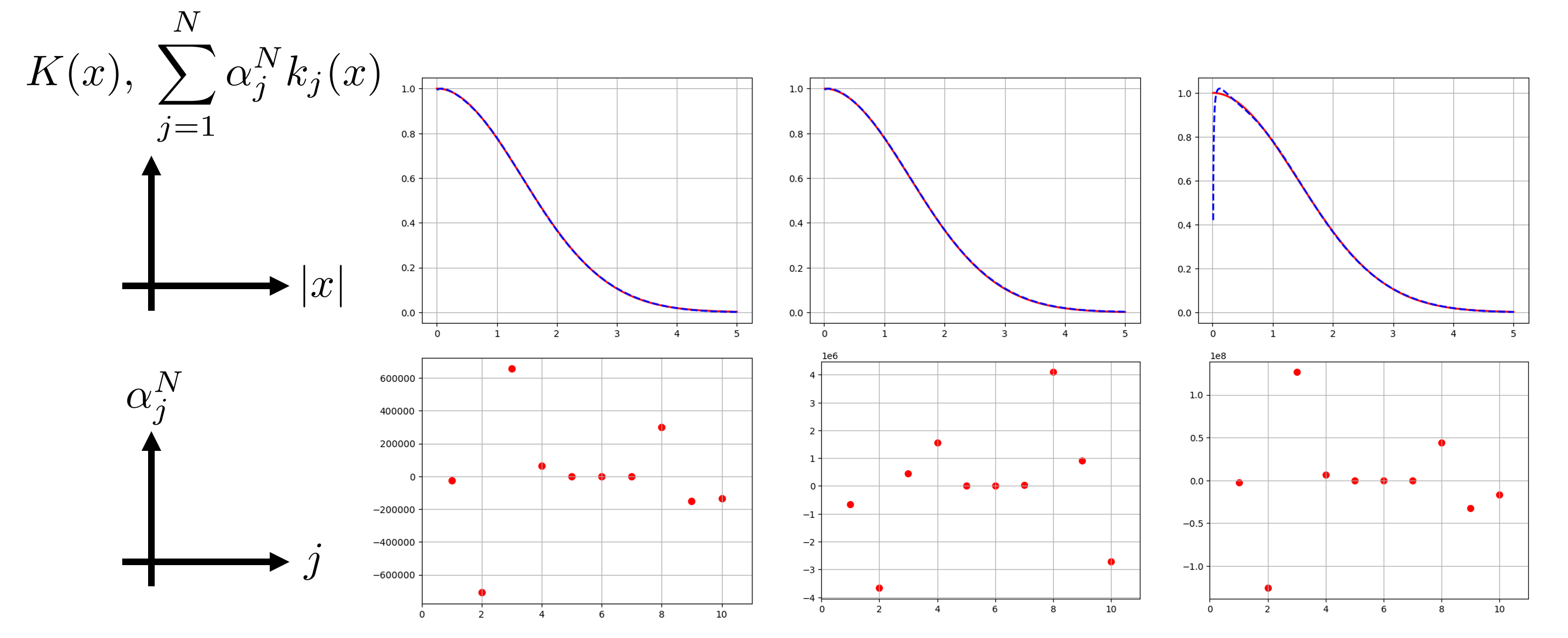
Figure 1. Graphs of $K(x)$ and $\sum^{N}_{j=1}\alpha^{N}_{j}k_{j}(x)$ with $N=10$ (top panels), the distributions of $\{\alpha_{j}\}_{1\leq j\leq N+1}$ (bottom panels). The graphs of $K(x)$ and $\sum^{N}_{j=1}\alpha^{N}_{j}k_{j}(x)$ are represented by the red curve and the blue dashed curve, respectively. The numerical examples are demonstrated for $n=1$ (left), $n=2$ (middle), and $n=3$ (right).

5. Concluding remarks

This paper clarifies a class of radial integral kernels that can be approximated by linear sums of the Green functions. It indicates that the nonlocal operator of convolution type with the kernel in the class can be described by a PDE system. In addition, a method for determining the coefficients in the case of $L^{2}({\mathbb{R}}^{n})$ with $n\leq 3$ is presented to illustrate the approximation by numerical calculations. Note that the determination of coefficients in other cases proceeds in essentially the similar manner. It should be remarked that the Green function does not belong to $L^{2}({\mathbb{R}}^{n})$ in the case of $n\geq 4$, nor to $H^{m}({\mathbb{R}}^{n})$ when $m\geq 2$ and $n\geq 1$. Thus, by replacing the basis with the linear sum (3.2) of the Green functions, the coefficients can be determined in a similar manner.

Recently, a constructive approximation of the same problem in $L^{1}({\mathbb{R}}^{n})$ for $n=1,2,3$ has been obtained by [18]. The result gives specific coefficients and accuracy of approximation by using the properties of the Green function depending on the dimension $n$. In the general dimension case, it is not yet known whether the approximation in $L^{1}({\mathbb{R}}^{n})$ is possible. If we proceed with the approach of this paper, one direction is to discuss completeness of the Green functions on a weighted Hilbert space that can be embedded in $L^{1}({\mathbb{R}}^{n})$, but it remains to a future problem whether we can proceed successfully or not.

References

• [1] S. Ai, R. Albashaireh, Traveling Waves in Spatial SIRS Models, J. Dyn. Diff. Equat. 26 (2014), 143-164.
• [2] T. Anderson, G. Faye, A. Scheel, D. Stauffer, Pinning and Unpinning in Nonlocal Systems, Journal of Dynamics and Differential Equations, 28 (2016), 897-923.
• [3] S. Amari, Dynamics of Pattern Formation in Lateral-Inhibition Type Neural Fields, Biol. Cybernetics, 27 (1977), 77-87.
• [4] F. Andreu-Vaillo, J. Mazón, J. D. Rossi, J. J. Toledo-Melero, Nonlocal diffusion problems, Math. Surveys Monogr. 165, AMS, Providence, RI, 2010.
• [5] P. Bates, On some nonlocal evolution equations arising in materials science, In: Nonlinear dynamics and evolution equations (Ed. by H. Brunner, X. Zhao and X. Zou), Fields Inst. Commun., AMS, Providence, 48 (2006), 13-52.
• [6] P. W. Bates, X. Chen, A. Chmaj, Heteroclinic solutions of a van der Waals model with indefinite nonlocal interactions, Calc. Var., 24 (2005), 261-281.
• [7] P. W. Bates, P. C. Fife, X. Ren, X. Wang, Traveling waves in a convolution model for phase transitions, Arch. Ration. Mech. Anal., 138 (1997), 105-136.
• [8] J. A. Carrillo, H. Murakawa, M. Sato, H. Togashi, O. Trush, A population dynamics model of cell-cell adhesion incorporating population pressure and density saturation, J. Theor. Biology, 474 (2019), 14-24.
• [9] X. Chen, Existence, uniqueness and asymptotic stability of traveling waves in nonlocal evolution equations, Adv. Differential Equations, 2(1) (1997), 125-160.
• [10] S. Coombes, H. Schmidt, I. Bojak, Interface dynamics in planar neural field models, The Journal of Mathematical Neuroscience, (2012) 2:9.
• [11] S.-I. Ei, J.-S. Guo, H. Ishii, C.-C. Wu, Existence of traveling waves solutions to a nonlocal scalar equation with sign-changing kernel, Jounal of Mathematical Analysis and Applications, 487(2), (2020), 124007.
• [12] S.-I. Ei, H. Ishii, The motion of weakly interacting localized patterns for reaction-diffusion systems with nonlocal effect, Discrete Contin. Dynam. Syst. Ser. B., 26(1) (2021), 173-190.
• [13] S.-I. Ei, H. Ishii, S. Kondo, T. Miura, Y. Tanaka, Effective nonlocal kernels on reaction-diffusion networks, Journal of Theoretical Biology, 509 (2021), 110496.
• [14] G. Faye, Existence and stability of traveling pulses of a neural field equation with synaptic depression, SIAM J. Appl. Dyn. Syst., 12 (2013), 2032-2067.
• [15] G. Faye and M. Holzer, Modulated traveling fronts for a nonlocal Fisher-KPP equation: a dynamical system approach, J. of Differential Equations, 258, (2015), 2257-2289.
• [16] S. Folias and P. Bressloff, Breathing Pulses in an Excitatory Neural Network, SIAM J. Applied Dynamical Systems, 3 (2004), 378-407.
• [17] V. Hutson, S. Martinez, K. Mischaikow, G.T. Vickers, The evolution of dispersal, J. Math. Biol. 47 (2003), 483-517.
• [18] H. Ishii, Y. Tanaka, Reaction-diffusion approximation of nonlocal interactions in higher-dimensional Euclidean space, preprint.
• [19] S. Kondo, An updated kernel-based Turing model for studying the mechanisms of biological pattern formation, J. Theoretical Biology, 414 (2017), 120-127.
• [20] C. Laing, W. Troy, PDE Methods for Nonlocal Models, SIAM J. Applied Dynamical Systems, 2 (2003), 487-516.
• [21] T. Li, Y. Li, H. Hethcote, Periodic traveling waves in SIRS endemic models, Mathematical and Computer Modelling, 49 (2009), 393-401.
• [22] H. Murakawa, Y. Tanaka, Keller-Segel type approximation for nonlocal Fokker-Planck equations in one-dimensional bounded domain, arXiv:2402.11511.
• [23] D. Mistroa, L. Rodriguesa, A. Schmidb, A mathematical model for dispersal of an annual plant population with a seed bank, Ecological Modelling, 188 (2005), 52-61.
• [24] J. Murray, Mathematical Biology, Springer-Verlag, Berlin, 1993.
• [25] H. Ninomiya, Y. Tanaka, H. Yamamoto, Reaction, diffusion and non-local interaction, J. Math. Biol. 75 (2017), 1203-1233.
• [26] H. Ninomiya, Y. Tanaka, H. Yamamoto, Reaction-diffusion approximation of nonlocal interactions using Jacobi polynomials, Japan J. Indust. Appl. Math. 35 (2018), 613-651.
• [27] K. J. Painter, J. M. Bloomfield, J. A. Sherratt and A. Gerisch, A nonlocal model for contact attraction and repulsion in heterogeneous cell populations, Bulletin of Mathematical Biology, 77 (2015), 1132-1165.
• [28] E. C. Titchmarsh, Introduction to the Theory of Fourier Integrals, Second edition, Oxford at the Clarendon Press, 1948.
• [29] G. N. Watson, A Treatise on the Theory of Bessel Functions, Second edition, Cambridge University Press, Cambridge, London and New York, 1944.