Statistics in a Backscatter Eddy Viscosity Turbulence Model

Abstract.

This paper addresses two significant drawbacks of an eddy viscosity turbulence model: the issue of excessive dissipation relative to energy input and the lack of a universal parameter specification. Considering the Baldwin-Lomax model with backscatter effects, we first prove the existence and uniqueness of global weak solutions under mild conditions. Our next result shows that this model maintains energy dissipation rates consistent with energy input, thereby avoiding over-dissipation and aligning with K41 phenomenology. Additionally, we propose a range for the model’s parameters.

1. Introduction

Eddy viscosity turbulence models, which intend to model averages instead of instantaneous of turbulent variables, are widely used for industrial, aeronautical, meteorological and oceanographical applications [P00, W06, BIL06]. As all classical eddy viscosity models [LN92, S07, S68, JL16], the Baldwin-Lomax model [BLM78] also has well recognized limitations in not modeling backscatter or complex turbulence not at statistical equilibrium. Rong, Layton and Zhao in [RLZ19] adopted the model to incorporate the effects of energy flow from fluctuations back to means (backscatter) for a fluid filling a domain with solid walls. The model is given by

(1.1) $$\begin{split}\partial_{t}\mathbf{u}+\beta^{2}\,\nabla\times(l^{2}(\mathbf{x})\nabla\times\partial_{t}\mathbf{u})+\nabla\cdot(\mathbf{u}\otimes\mathbf{u})-&\nu\Delta\mathbf{u}+\nabla\times(l^{2}(\mathbf{x})|\nabla\times\mathbf{u}|\nabla\times\mathbf{u})+\nabla q=\mathbf{f},\\ &\nabla\cdot\mathbf{u}=0,\end{split}$$

with an initial condition $\mathbf{u}_{0}(\mathbf{x})$, where $\beta$ is a positive model calibration parameter, and $l(\mathbf{x})$ is a mixing length that depends on the distance to the wall, $0\leq l(\mathbf{x})\rightarrow 0$ as $\mathbf{x}\rightarrow\partial\Omega$. In the above $\mathbf{u}(\mathbf{x},t)$ and $q(\mathbf{x},t)$ approximate the true averages Navier-Stokes velocity and pressure respectively. The kinematic viscosity is denoted by $\nu$, and $\mathbf{f}$ is the known body force. It is shown in [RLZ19] that the eddy viscosity term $\nabla\times(l^{2}(\mathbf{x})|\nabla\times\mathbf{u}|\nabla\times\mathbf{u})$ accounts for the dissipative effect of the Reynolds stress. In addition, there is a two-dimensional computational test that indicates the non-smoothing dispersive term, $\beta^{2}\,\nabla\times(l^{2}(\mathbf{x})\nabla\times\partial_{t}\mathbf{u})$, accounts for statistical backscatter , however there is no artificial negative viscosity.

There are two common drawbacks shared by many eddy viscosity models. One is that model dissipation often exceeds the energy input, leading to non-physical solutions with higher viscosity. Another issue is the lack of a simple, universal, and effective specification of parameters, such as $\beta$ and $l(\mathbf{x})$ in (1.1), as they vary from case to case. In this manuscript, these two concerns are addressed through rigorous mathematical analysis, supported by computational evidence.

Herein, we first study the existence and uniqueness of the global weak solution to the equations (1.1), see Theorems 4.5 and 4.6. We show that, under mild condition on $\l(x)$, existence and uniqueness of solutions hold for the model. Another main result of this paper, Theorem 5.1, is that for the backscatter Baldwin-Lomax model (1.1) equipped with the Dirichlet boundary condition, the over dissipation does not happen: the model’s energy dissipation rate is consistent with its energy input rate, and that the model produces time averaged energy dissipation rates consistent with the K41 phenomenology given in [K41]. In addition, based on the analysis, a range for the mixing length is proposed, $\l(\mathbf{x})\sim\text{Re}^{-{1/2}}$, which is also consistent with the suggested mixing length in [W06].

1.1. Related works

Studies of turbulence typically rely on statistical rather than pointwise descriptions, as providing a detailed account of fluid behavior in a turbulent region is impractical due to the chaotic structures spanning a wide range of length scales. One such statistical quantity is the time-averaged energy dissipation rate [H72]. Based on Kolmogorov’s conventional turbulence theory at large Reynolds number, the energy dissipation rate per unit volume $\langle\varepsilon\rangle$ should be independent of the kinematic viscosity $\nu$, see [K41]. In other words, dissipation appears to exist independently of viscosity in zero limit. By a dimensional consideration, the energy dissipation rate per unit volume scales as

$$\langle\varepsilon\rangle\simeq C_{\varepsilon}\frac{U^{3}}{L},$$

where $U$ and $L$ are global velocity and length scales, with $C_{\varepsilon}=$ the asymptotic constant (Kolmogorov 1941). This result is fundamental to an understanding of turbulence [S68].

In the theory of turbulence, upper estimates of energy dissipation rates are useful for, in particular, overall complexities of turbulent flow simulations. It also determines the smallest persistent length scales and the dimension of any global attractor (if it exists) [DFJ09, F95]. Doering and Constantin in [DC92] and Doering and Foias in [DF02] proved rigorous asymptotic upper bounds directly from the Navier-Stokes equations. Their bound is of the form

$$\varepsilon\lesssim\frac{U^{3}}{h},\hskip 14.22636pt\text{as}\hskip 2.84544pt\ \text{Re}\to\infty,\hskip 14.22636pt\text{where}\hskip 5.69046pt\text{Re}=\frac{UL}{\nu}.$$

These works has developed in many important directions, e.g., [AP17, AP19, AP20, W97, W00, W10, L02, L16, DR00, FS1, FS2] for the deterministic flows. Very recently, the effect of randomness on the dissipation rate is studied in [fan20233d] and [FJP21] when noise is added on a boundary of shear flow. The authors in [CP20] could also prove $\mathcal{O}\left(U^{3}/L\right)$ lower bound for stochastically forced flows under an additional assumption of energy balance.

Organization of this paper

In Section 2, we introduce some standard notations and preliminaries. Section 3 revisits the corrected model (1.1), and we present definitions and the setting for the analysis. Later in Section 4, we discuss the existence and uniqueness results. Then in Section 5, we prove the central results of these considerations, that the dissipation rate is independent of the viscosity at high Reynolds number. Numerical experiments, demonstrating and extending beyond the analytical results, are described in Section 6.

2. Notation & preliminaries

Let $\Omega\subset\mathbb{R}^{3}$ be a bounded open domain with the volume $|\Omega|$ and $\mathbf{x}=(x_{1},x_{2},x_{3})\in\mathbb{R}^{3}$. Constant $C$ represents a generic positive constant independent of $\nu,\text{Re},$ and other model parameters.

Let $p\in[1,\infty]$, and the Lebesgue space $L^{p}(\Omega)$ is the space of all measurable functions $\mathbf{v}$ on $\Omega$ for which

$$\|\mathbf{v}\|_{L^{p}}:=\big{(}\int_{\Omega}|\mathbf{v}(\mathbf{x})|^{p}\,d\mathbf{x}\big{)}^{\frac{1}{p}}\,<\infty,\hskip 28.45274pt\text{if}\hskip 5.69046ptp\in[1,\infty),$$

$$\|\mathbf{v}\|_{L^{\infty}}:=\sup_{\mathbf{x}\in\Omega}|\mathbf{v}(\mathbf{x})|<\infty,\hskip 28.45274pt\text{if}\hskip 5.69046ptp=\infty.$$

The $L^{2}$ norm and inner product will be denoted by $\|\cdot\|$ and $(\cdot,\cdot)$ respectively, while all other norms will be labeled with subscripts. Let $\mathbf{V}$ be a Banach space of functions defined on $\Omega$ with the associated norm $\|\cdot\|_{\mathbf{V}}$. We denote by $L^{p}(a,b;\mathbf{V})$, $p\in[1,\infty]$, the space of functions $\mathbf{v}:(a,b)\rightarrow\mathbf{V}$ such that

$$\|\mathbf{v}\|_{L^{p}(a,b;\mathbf{V})}:=\big{(}\int_{a}^{b}\|\mathbf{v}(t)\|_{\mathbf{V}}^{p}\,d\mathbf{x}\big{)}^{\frac{1}{p}}\,<\infty,\hskip 28.45274pt\text{if}\hskip 5.69046ptp\in[1,\infty),$$

$$\|\mathbf{v}\|_{L^{\infty}(a,b;\mathbf{V})}:=\sup_{t\in(a,b)}\|\mathbf{v}(t)\|_{\mathbf{V}}<\infty,\hskip 28.45274pt\text{if}\hskip 5.69046ptp=\infty.$$

The space $H^{-1}$ is dual to $H^{1}$, and its norm is defined as

$$\|\mathbf{v}\|_{-1}=\sup_{\phi\in H^{1}}\frac{|(\mathbf{v},\phi)|}{\|\nabla\phi\|}.$$

The space $W_{0}^{1,p}(\Omega)$ consists of all functions in $W^{1,p}$ which vanish on the boundary $\partial\Omega$ (in the sense of traces)

$$W_{0}^{1,p}=\big{\{}\mathbf{v}:\hskip 2.84544pt\mathbf{v}\in W^{1,p}(\Omega)\hskip 8.5359pt\text{and}\hskip 8.5359pt\mathbf{v}|_{\partial\Omega}=0\big{\}}.$$

Moreover

$$W_{0,div}^{1,p}=\big{\{}\mathbf{v}:\hskip 2.84544pt\mathbf{v}\in W_{0}^{1,p}(\Omega)\hskip 8.5359pt\text{and}\hskip 8.5359pt\nabla\cdot\mathbf{v}=0\big{\}}.$$

Some inequalities

Let $1\leq p\leq\infty$; we denote by $q$ the conjugate exponent, $\frac{1}{p}+\frac{1}{q}=1$. Assume that $f\in L^{p}$ and $g\in L^{q}$ with $1\leq p\leq\infty$. Then $fg\in L^{1}$ and

(Höler inequality) $$\|fg\|_{L^{1}}\leq\|f\|_{L^{p}}\,\|g\|_{L^{q}}$$

Moreover, for any $a,b\geq 0$ and $\lambda>0$ we have

(Young inequality) $$ab\leq\frac{\lambda^{-\frac{p}{q}}\,a^{p}}{p}+\frac{\lambda\,b^{q}}{q}.$$

There is a constant $C_{\text{P}}$ depends on $\Omega$ such that for any $\mathbf{u}\in H_{0}^{1}(\Omega)^{3},$

(Poincaré inequality) $$\|\mathbf{u}\|\leq C_{\text{P}}\|\nabla\mathbf{u}\|.$$

In the sequel, we will make use of the classical embedding theorems for Sobolev spaces in $d=3$,

(Sobolev embedding) $$\begin{split}&W^{1,p}(\Omega)\hookrightarrow L^{6}(\Omega),\quad\forall\,p\in[2,\infty).\\ &W^{1,3}(\Omega)\hookrightarrow L^{p}(\Omega),\quad\forall\,p\in[1,\infty).\end{split}$$

Before presenting the main results, we report the following Grönwall lemmas which were first mentioned in [G19] by T. Hakon Grönwall.

Proposition 2.1 (Grönwall’s lemma: Integral form).

Let $T\in\mathbb{R}^{+}\cup\{\infty\}$ and $\alpha,\beta\in L^{\infty}(0,T)$ with $\lambda\in L^{1}(0,T),\lambda(t)\geq 0$, for almost all $t\in[0,T]$. Then

$$\alpha(t)\leq\beta(t)+\int_{0}^{t}\lambda(s)\,\alpha(s)\,ds\hskip 28.45274pt\text{a.e. in }[0,T],$$

implies for almost all $t\in[0,T]$

$$\alpha(t)\leq\beta(t)+\int_{0}^{t}e^{\gamma(t)-\gamma(s)}\,\lambda(s)\,\beta(s)\,ds,$$

where $\gamma(t):=\int_{0}^{t}\lambda(\tau)\,d\tau$. If $\beta\in W^{1,1}(0,T)$, it follows

$$\alpha(t)\leq e^{\gamma(t)}\,\left(\beta(0)+\int_{0}^{t}e^{-\gamma(s)}\,\beta^{\prime}(s)\,ds\right).$$

Moreover, if $\beta$ is a monotonically increasing, continuous function, it holds,

$$\alpha(t)\leq e^{\gamma(t)}\,\beta(t).$$

Proposition 2.2 (Gronwall’s lemma in differential form).

Let $T\in\mathbb{R}^{+}\cup\{\infty\}$, $\alpha\in W^{1,1}(0,T)$ and $\beta,\,\lambda\in L^{1}(0,T)$. Then

$$\alpha^{\prime}(t)\leq\beta(t)+\lambda(t)\,\alpha(t)\hskip 28.45274pt\text{a.e. in }[0,T]$$

implies for almost all $t\in[0,T]$

$$\alpha(t)\leq\alpha(0)\,e^{\left[\int_{0}^{t}\,\lambda(\tau)\,d\tau\right]}+\int_{0}^{t}\,\beta(s)\,e^{\left[\int_{s}^{t}\lambda(\tau)\,d\tau\right]}\,ds.$$

Lastly, we would like to highlight an important property of the eddy viscosity term that will be valuable in the subsequent analysis. The proof of this property can be found in [RLZ19].

Proposition 2.3 (Strong monotonicity).

For all $\mathbf{u},\mathbf{u}^{\prime}\in W^{1,3}(\Omega)$, there is a constant $\tilde{c}>0$ such that

$$\left(l^{2}(\mathbf{x})|\nabla\times\mathbf{u}|\nabla\times\mathbf{u}-l^{2}(\mathbf{x})|\nabla\times\mathbf{u}^{\prime}|\nabla\times\mathbf{u}^{\prime}\,,\,\nabla\times(\mathbf{u}-\mathbf{u}^{\prime})\right)\geq\tilde{c}\,\|\l^{\frac{3}{2}}(x)\,\nabla\times(\mathbf{u}-\mathbf{u}^{\prime})\|_{L^{3}}^{3}.$$

3. The rotational backscatter model

One of the most used approaches in simulating turbulent flows is to model the ensemble-averaged Navier–Stokes equations by eddy viscosity, and then solve the discretized result. To begin, consider the incompressible Navier–Stokes equations (NSE) driven by a known body force $\mathbf{f}(\mathbf{x},t)$ and starting from an initial condition $\mathbf{v}(\mathbf{x},0)=\mathbf{v}_{0}(\mathbf{x})$

(3.1) $$\begin{split}\partial_{t}\mathbf{v}+\nabla\cdot(\mathbf{v}\otimes\mathbf{v})-&\nu\,\Delta\mathbf{v}+\nabla p=\mathbf{f},\hskip 5.69046pt\text{and}\hskip 5.69046pt\nabla\cdot\mathbf{v}=0\hskip 5.69046pt\text{in}\,\Omega,\\ &\mathbf{v}=0\hskip 5.69046pt\text{on}\hskip 4.26773pt\partial\Omega,\hskip 12.80365pt\text{and}\hskip 4.26773pt\int_{\Omega}p\,d\mathbf{x}=0.\end{split}$$

Here, $\Omega\subset\mathbb{R}^{3}$ is a bounded polyhedral domain, $\mathbf{v}:\Omega\times[0;T]\rightarrow\mathbb{R}^{3}$ is the fluid velocity and $p:\Omega\times(0;T]\rightarrow\mathbb{R}$ is the fluid pressure. Due to measurement imprecision in input data (e.g., initial velocity), we consider ensemble of $J$ Navier–Stokes equations. Let $\mathbf{v}(\mathbf{x},t;\omega_{j}),\,p(\mathbf{x},t;\omega_{j})$ be associated solutions to the NSE (3.1) given an ensemble of initial conditions

$$\mathbf{v}(\mathbf{x},0;\omega_{j})=\mathbf{v}_{0}(\mathbf{x};\omega_{j}),\hskip 28.45274ptj=1,...,J.$$

Then the instantaneous velocity filed and pressure are decomposed into the mean and fluctuating components

$$\mathbf{v}=\langle\mathbf{v}\rangle+\mathbf{v}^{\prime},\hskip 14.22636pt\text{and}\hskip 14.22636ptp=\langle p\rangle+p^{\prime},$$

where the ensemble means are

$$\langle\mathbf{v}\rangle\,(\mathbf{x},t):=\frac{1}{J}\,\sum_{j=1}^{J}\mathbf{v}(\mathbf{x},t;\omega_{j}),\hskip 14.22636pt\text{and}\hskip 14.22636pt\langle p\rangle\,(\mathbf{x},t):=\frac{1}{J}\,\sum_{j=1}^{J}p(\mathbf{x},t;\omega_{j}),$$

and fluctuations about the mean are given by

$$\mathbf{v}^{\prime}(\mathbf{x},t;\omega_{j}):=\mathbf{v}(\mathbf{x},t;\omega_{j})-\langle\mathbf{v}\rangle\,(\mathbf{x},t),\hskip 14.22636pt\text{and}\hskip 14.22636ptp^{\prime}(\mathbf{x},t;\omega_{j}):=p(\mathbf{x},t;\omega_{j})-\langle p\rangle\,(\mathbf{x},t).$$

After introducing the above decomposition into the equations (3.1), one can obtain the ensemble averaging equations, which form a non-closed system

(3.2) $$\partial_{t}\langle\mathbf{v}\rangle+\langle\mathbf{v}\rangle\cdot\nabla\langle\mathbf{v}\rangle-\nu\,\Delta\langle\mathbf{v}\rangle-\nabla\cdot\mathbf{R}\,(\mathbf{v},\mathbf{v})+\nabla\langle p\rangle=\mathbf{f},\hskip 5.69046pt\text{and}\hskip 5.69046pt\nabla\cdot\langle\mathbf{u}\rangle=0\hskip 5.69046pt\text{in}\,\Omega,\\$$

where the Reynolds stress $\mathbf{R}\,(\mathbf{v},\mathbf{v})$ is

$$\mathbf{R}\,(\mathbf{v},\mathbf{v}):=\langle\mathbf{v}\rangle\otimes\langle\mathbf{v}\rangle-\langle\mathbf{v}\otimes\mathbf{v}\rangle=-\langle\mathbf{v}^{\prime}\otimes\mathbf{v}^{\prime}\rangle.$$

By invoking the Boussinesq conjecture and eddy viscosity hypothesis, the Reynolds stress is modeled by

$$-\nabla\cdot\mathbf{R}\,(\mathbf{v},\mathbf{v})\sim-\nabla\cdot\left(\nu_{T}\left(\langle\mathbf{v}\rangle\right)\,\nabla\left(\langle\mathbf{v}\rangle\right)\right)+\text{terms incorporated into the new pressure},$$

and the standard eddy viscosity (EV) model is given by

(3.3) $$\begin{split}\partial_{t}\mathbf{u}+\nabla\cdot(\mathbf{u}\otimes\mathbf{u})-&\nu\,\Delta\mathbf{u}-\nabla\cdot\big{(}\nu_{T}(\mathbf{u})\,\nabla\mathbf{u}\big{)}+\nabla q=\mathbf{f},\\ &\nabla\cdot\mathbf{u}=0.\end{split}$$

Since (3.3) is a model, its solution is no longer the exact ensemble average, and solutions $\mathbf{u}(\mathbf{x},t)$ and $q(x,t)$ are intended to approximate the true average velocity $\langle\mathbf{v}\rangle$ and pressure $\langle p\rangle$ receptively.

The turbulent viscosity coefficient $\nu_{T}(\langle\mathbf{u}\rangle)$ should be calibrated by fitting it to flow data, and many parameterizations of eddy viscosity models are known, e.g. [BIL06, CL14, J06, LL02, MP94, V04]. In the simplified Baldwin-Lomax model [BLM78], the eddy viscosity coefficient calibrated as

(3.4) $$\nu_{T}(\mathbf{u})=l^{2}(\mathbf{x})|\nabla\times\mathbf{u}|,$$

where $l(\mathbf{x})$ is a multiple of the distance from the boundary. Existence of weak solutions for the Baldwin-Lomax model in the steady case is recently proved in [BB20]. By looking into the energy equation, since $\nu_{T}>0$ in the above calibration (3.4), the the eddy viscosity term $-\nabla\cdot\big{(}\nu_{T}(\mathbf{u})\,\nabla\mathbf{u}\big{)}$ in (3.3) can only characterize the dissipation effects of the Reynolds stress and is unable to represent the backscatter. Like many EV models [LN92, S07, S68, JL16], the basic Baldwin-Lomax model has difficulty with complex turbulence not at statistical equilibrium. It performs poorly in simulating backscatter, and is unable to model effects such as separations and wakes.

After expressing the eddy viscosity term in rotational (curl-curl) form, the authors in [RLZ19] adopted the Baldwin-Lomax model to non equilibrium turbulence, and introduced the backscatter rotational model (1.1). The derivation of the model is based on the variance evolution equation, and the approach suggested in [JL16] (for more details see [RLZ19] Section 3). It is proved that the effects of terms that modeled the Reynolds stress are dissipative in long time averaging sense

$$\liminf_{T\rightarrow\infty}\frac{1}{T}\,\int_{0}^{T}\,\int_{\Omega}\left(\beta^{2}l^{2}(\mathbf{x})\nabla\times\mathbf{u}_{t}\,\cdot\,\nabla\times\mathbf{u}+l^{2}(\mathbf{x})|\nabla\times\mathbf{u}|^{3}\right)\,d\mathbf{x}\,dt\geq 0,$$

while there are numerical evidences (see Figures 3, 4, 5, and 6 in [RLZ19]) that indicate the backscatter occurs and energy is transferred from fluctuations to the mean at some times.

Existence and uniqueness of the weak solution is discussed in the following sections, and one can show that the solution satisfy the energy inequality

(3.5) $$\frac{1}{2}\frac{d}{dt}\,\left(\,\|\mathbf{u}\|^{2}+\beta^{2}\|\l(x)\,\nabla\times\mathbf{u}\|^{2}\,\right)+\nu\|\nabla\mathbf{u}\|^{2}+\int_{\Omega}l^{2}(x)|\nabla\times\mathbf{u}|^{3}\,d\mathbf{x}\leq(\mathbf{f},\mathbf{u}).$$

Remark 3.1.

After dividing the both sides of (3.5) by the volume of domain $|\Omega|$, we can identify the following quantities

• Model kinetic energy of mean flow per unit volume

  $$\mbox{MKE}:=\frac{1}{2}\frac{1}{|\Omega|}\,\frac{d}{dt}\,\left(\,\|\mathbf{u}\|^{2}+\beta^{2}\|\l(x)\,\nabla\times\mathbf{u}\|^{2}\,\right),$$

• Rate of energy dissipation of mean flow per unit volume

  $$\varepsilon(t):=\frac{\nu}{|\Omega|}\,\|\nabla\mathbf{u}\|^{2}+\frac{1}{|\Omega|}\,\int_{\Omega}l^{2}(x)|\nabla\times\mathbf{u}|^{3}\,d\mathbf{x},$$

• Rate of energy input to mean flow per unit volume

  $$\frac{1}{|\Omega|}\,(\mathbf{f},\mathbf{u}).$$

Definition 3.2.

The dissipation quantities (per unit volume) are given as

$$\varepsilon_{0}:=\frac{1}{|\Omega|}\int_{\Omega}\nu|\nabla\mathbf{u}|^{2}d\mathbf{x}=\frac{1}{|\Omega|}\nu\|\nabla u\|^{2},$$

$$\varepsilon_{M}:=\frac{1}{|\Omega|}\int_{\Omega}l^{2}(\mathbf{x})|\nabla\times\mathbf{u}|^{3}d\mathbf{x}.$$

The long time average of a function $\phi(t)$ is defined

$$\langle\phi\rangle:=\limsup_{T\rightarrow\infty}\frac{1}{T}\,\int_{0}^{T}\,\phi(t)\,dt.$$

The time-averaged energy dissipation rate (per volume) for model (1.1) includes dissipation due to the viscous forces and turbulent diffusion. It is given by

(3.6) $$\langle\varepsilon\rangle:=\limsup_{T\rightarrow\infty}\frac{1}{T}\,\int_{0}^{T}\,\varepsilon_{0}+\varepsilon_{M}\,dt.$$

4. On the existence and uniqueness of weak solutions

In this section we prove existence and uniqueness of (weak) solutions to (1.1). We assume that $\mathbf{u}$ is a sufficiently regular solution of the equations (1.1), and then establish a priori estimates on $\mathbf{u}$ in the the subsequent lemmas. In this context, our approach involves working in a formal manner. However, it is important to highlight that the formal derivation, along with the accompanying a priori estimates, can be rigorously established by employing a Galerkin approximation. Given the standard nature of this approach, which holds true for both the 2D and 3D Navier-Stokes (NS) system, as well as other turbulence models like the Smagorinsky [S63] and Ladyzhynskaya model [L63], we have chosen to omit the intricate details at this juncture. Instead, we kindly refer readers seeking more comprehensive discussions to the following references: [MNR01, T77], as well as the supplementary references contained within.

Assumption 4.1.

Throughout the remainder of the manuscript, we assume the following regularity conditions on the external force $\mathbf{f}$, initial condition $\mathbf{u}_{0}$ and the model parameter $\l(x)$,

(4.1) $$\mathbf{u}_{0}\in W_{0,div}^{1,3},\hskip 14.22636pt\mathbf{f}\in L^{2}(0,T;L^{2}(\Omega)),\hskip 14.22636pt0<\l_{0}\leq\l(x)\leq\l_{max}.$$

Before proving the main theorems, we need to prove boundedness of the kinetic energy, and that $\langle\varepsilon\rangle$ is well-defined in the following proposition.

Proposition 4.2.

Under the above regularity assumptions (4.1), the kinetic energy and the time-averaged of the energy dissipation of the solution to (1.1) are uniformly bounded in time. Moreover

(4.2) $$\mathbf{u}\hskip 5.69046pt\text{and}\hskip 5.69046ptl(\mathbf{x})\nabla\times\mathbf{u}\in L^{\infty}(0,\infty;L^{2}).$$

Proof.

Using Poincaré inequality together with the Grönwall inequality in (3.5) implies that the kinetic energy is uniformly bounded in time according to

$$\|\mathbf{u}(t)\|^{2}+\beta^{2}\|\l(\mathbf{x})\,\nabla\times\mathbf{u}(t)\|^{2}\leq\big{(}\|\mathbf{u}(0)\|^{2}+\beta^{2}\|\l(\mathbf{x})\,\nabla\times\mathbf{u}(0)\|^{2}\big{)}\,e^{-\alpha t}+\frac{1}{\alpha\,\nu}\|\mathbf{f}\|^{2}_{L^{2}(0,t;H^{-1})}\,(1-e^{-\alpha t}),$$

for any $0<t<\infty$, where $\alpha=\min\{\frac{\nu}{2C_{\text{P}}},\frac{\nu}{2\beta^{2}\,\ell_{\text{max}}}\}>0$, for more details see [RLZ19]. Hence, for a constant $C$ depending on the given data $\mathbf{u}_{0}$ and $\mathbf{f}$,

(4.3) $$\begin{split}&\sup_{t\in[0,\infty]}\|\mathbf{u}(t)\|^{2}\leq C<\infty,\\ &\sup_{t\in[0,\infty]}\|\l(\mathbf{x})\,\nabla\times\mathbf{u}(t)\|^{2}\leq C<\infty.\end{split}$$

Now Young inequality for $p=q=2$, and $\lambda=\sqrt{2\nu}$, the right-hand side of (3.5) is majorized by

$$(\mathbf{f},\mathbf{u})\leq\|\mathbf{f}\|_{H^{-1}}\,\|\mathbf{u}\|_{H^{1}}\leq\frac{1}{4\,\nu}\|\mathbf{f}\|^{2}_{H^{-1}}+\nu\|\nabla\mathbf{u}\|^{2}.$$

Therefore,

$$\frac{d}{dt}\,\big{(}\|\mathbf{u}\|^{2}+\beta^{2}\|\l(x)\,\nabla\times\mathbf{u}\|^{2}\big{)}+\nu\|\nabla\mathbf{u}\|^{2}+2\int_{\Omega}l^{2}(x)|\nabla\times\mathbf{u}|^{3}\,d\mathbf{x}\leq\frac{1}{4\,\nu}\|\mathbf{f}\|^{2}_{H^{-1}}.$$

Integrating above for $0$ to $T$, we obtain in particular

(4.4) $$\begin{split}\|\mathbf{u}(T)\|^{2}+\beta^{2}\|\l(x)\,\nabla\times\mathbf{u}(T)\|^{2}&+\int_{0}^{T}\nu\|\nabla\mathbf{u}\|^{2}dt+2\int_{0}^{T}\int_{\Omega}l^{2}(x)|\nabla\times\mathbf{u}|^{3}\,d\mathbf{x}\,dt\\ &\leq\|\mathbf{u}(0)\|^{2}+\beta^{2}\|\l(x)\,\nabla\times\mathbf{u}(0)\|^{2}+\frac{1}{4\,\nu}\,\|\mathbf{f}\|^{2}_{L^{2}(0,T;H^{-1})}\\ &=:c_{1}(T).\end{split}$$

Now taking the limit superior from above, and using (4.2), one can also show that $\langle\varepsilon\rangle$ is well-defined.

∎

Lemma 4.3.

Under the regularity conditions specified in Assumption 4.1, we have

$$\mathbf{u}\in L^{2}(0,T;H^{1}(\Omega))\cap L^{3}(0,T;W^{1,3}(\Omega)).$$

Proof.

The result is concluded from (4.4). ∎

Lemma 4.4.

Under the regularity conditions specified in Assumption 4.1, we have

$$\|\nabla\times\mathbf{u}(T)\|_{L^{3}}^{3}\leq c_{2}(T).$$

Proof.

One starts by testing the momentum equation (1.1) with $\partial_{t}\mathbf{u}$. This gives, after integration on $(0,T)$ and integration by parts

(4.5) $$\begin{split}&\int_{0}^{T}\left(\|\partial_{t}\mathbf{u}\|^{2}+\beta^{2}\|\l(x)\nabla\times\partial_{t}\mathbf{u}\|^{2}\right)\,dt+\frac{\nu}{2}\|\nabla\mathbf{u}(T)\|^{2}+\frac{1}{3}\|\l(x)^{\frac{2}{3}}\,\nabla\times\mathbf{u}(T)\|_{L^{3}}^{3}\\ &=\frac{\nu}{2}\|\nabla\mathbf{u}_{0}\|^{2}+\frac{1}{3}\|\l(x)^{\frac{2}{3}}\,\nabla\times\mathbf{u}_{0}\|_{L^{3}}^{3}-\int_{0}^{T}(\mathbf{u}\cdot\nabla\mathbf{u},\partial_{t}\mathbf{u})\,dt+\int_{0}^{T}(\mathbf{f},\partial_{t}\mathbf{u})\,dt.\end{split}$$

Using the equivalency of the $L^{p}$ norms for $\nabla\mathbf{u}$ and $\nabla\times\mathbf{u}$, with Höler inequality and Sobolev embedding gives

$$\begin{split}\int_{\Omega}(\mathbf{u}\cdot\nabla\mathbf{u})^{2}\,d\mathbf{x}\leq\|\nabla\mathbf{u}\|_{L^{3}}^{2}\,\|\mathbf{u}\|_{L^{6}}^{2}\leq c\,\|\nabla\mathbf{u}\|_{L^{3}}^{4}\leq c\,\|\nabla\times\mathbf{u}\|_{L^{3}}^{4}.\end{split}$$

With the above bound, the convective term can be estimated as

$$\begin{split}\int_{0}^{T}\left(\mathbf{u}\cdot\nabla\mathbf{u},\partial_{t}\mathbf{u}\right)dt&\leq\int_{0}^{T}\int_{\Omega}\frac{1}{4}(\partial_{t}\mathbf{u})^{2}+(\mathbf{u}\cdot\nabla\mathbf{u})^{2}\,d\mathbf{x}\,dt\\ &\leq\frac{1}{4}\int_{0}^{T}\|\partial_{t}\mathbf{u}\|^{2}dt+c\int_{0}^{T}\|\nabla\times\mathbf{u}\|_{L^{3}}^{4}dt.\end{split}$$

The force term can be esteemed as

$$\int_{0}^{T}(\mathbf{f},\partial_{t}\mathbf{u})\,dt\leq\int_{0}^{T}\|\mathbf{f}\|^{2}+\frac{1}{4}\|\partial_{t}\mathbf{u}\|^{2}\,dt.$$

Then by combining all the above estimates, we obtain

(4.6) $$\begin{split}&\int_{0}^{T}\left(\|\partial_{t}\mathbf{u}\|^{2}+2\beta^{2}\|\l(x)\nabla\times\partial_{t}\mathbf{u}\|^{2}\right)\,dt+\nu\|\nabla\mathbf{u}(T)\|^{2}+\frac{2}{3}\|\l(x)^{\frac{2}{3}}\,\nabla\times\mathbf{u}(T)\|_{L^{3}}^{3}\\ &\leq\nu\|\nabla\mathbf{u}_{0}\|^{2}+\frac{2}{3}\|\l(x)^{\frac{2}{3}}\,\nabla\times\mathbf{u}_{0}\|_{L^{3}}^{3}+2\int_{0}^{T}\|\mathbf{f}\|^{2}dt+c\int_{0}^{T}\|\nabla\times\mathbf{u}\|_{L^{3}}^{4}dt.\end{split}$$

In particular with $\l_{0}\leq\l(x)\leq\l_{1}$, we have

(4.7) $$\begin{split}\|\nabla\times\mathbf{u}(T)\|_{L^{3}}^{3}&\leq\frac{3}{4}\frac{\nu}{\l_{0}^{2}}\|\nabla\mathbf{u}_{0}\|^{2}+\frac{1}{\l_{0}^{2}}\|\l(x)^{\frac{2}{3}}\,\nabla\times\mathbf{u}_{0}\|_{L^{3}}^{3}+\frac{3}{\l_{0}^{2}}\int_{0}^{T}\|\mathbf{f}\|^{2}dt\\ &+\frac{c}{\l_{0}^{2}}\int_{0}^{T}\|\nabla\times\mathbf{u}\|_{L^{3}}^{4}dt.\end{split}$$

The application of Grönwall lemma (Proposition 2.1) gives

(4.8) $$\begin{split}\|\nabla\times\mathbf{u}(T)\|_{L^{3}}^{3}&\leq\left(\frac{3}{4}\frac{\nu}{\l_{0}^{2}}\|\nabla\mathbf{u}_{0}\|^{2}+\frac{1}{\l_{0}^{2}}\|\l(x)^{\frac{2}{3}}\,\nabla\times\mathbf{u}_{0}\|_{L^{3}}^{3}+\frac{3}{\l_{0}^{2}}\int_{0}^{T}\|\mathbf{f}\|^{2}dt\right)\\ &\times\exp\left(\frac{c}{\l_{0}^{2}}\int_{0}^{T}\|\nabla\times\mathbf{u}\|_{L^{3}}dt\right).\end{split}$$

Using the result in Lemma 4.3, we can estimate the term in exponential as

$$\int_{0}^{T}\|\nabla\times\mathbf{u}\|_{L^{3}}\,dt\leq T^{\frac{2}{3}}\,\left(\int_{0}^{T}\|\nabla\times\mathbf{u}\|_{L^{3}}^{3}\,dt\right)^{\frac{1}{3}}\leq T^{\frac{2}{3}}\,\left(c_{1}(T)\right)^{\frac{1}{3}},$$

which proves the lemma. ∎

Having the above estimates in hand, we employ the Galerkin approximation scheme to obtain the existence of weak solutions, as stated in the next theorem, using standard arguments. We refer the reader to [MNR01, T77] for a detailed argument for the passage of limit.

Theorem 4.5 (Existence of a weak solution).

Given the regularity conditions outlined in Assumption 4.1, there exists a weak solution $\mathbf{u}$ to (1.1) satisfying

$$\mathbf{u}\in L^{\infty}(0,T;L^{2}(\Omega))\cap L^{2}(0,T;H^{1}(\Omega))\cap L^{3}(0,T;W_{0,div}^{1,3}(\Omega)),$$

for all $T>0$.

Theorem 4.6 (Uniqueness of the weak solution).

Given the regularity conditions outlined in Assumption 4.1, the weak solution of (1.1) is unique.

Proof.

Let us assume that there are two weak solutions $\mathbf{u}$ and $\mathbf{u}^{\prime}$ guaranteed by Theorem 4.5 with $\mathbf{u}_{0}=\mathbf{u}^{\prime}_{0}$, and denote $\mathbf{w}=\mathbf{u}-\mathbf{u}^{\prime}$. Thus $\mathbf{w}\in W^{1,3}(\Omega)$ and $\mathbf{w}_{0}=0$, and the error function satisfies

$$\begin{split}\frac{1}{2}\frac{d}{dt}&\,\left(\,\|\mathbf{w}\|^{2}+\beta^{2}\|\l(x)\,\nabla\times\mathbf{w}\|^{2}\,\right)+\nu\|\nabla\mathbf{w}\|^{2}+\left(\mathbf{u}\cdot\nabla\mathbf{u}-\mathbf{u}^{\prime}\cdot\nabla\mathbf{u}^{\prime},\mathbf{w}\right)\\ &+\left(l^{2}(\mathbf{x})|\nabla\times\mathbf{u}|\nabla\times\mathbf{u}-l^{2}(\mathbf{x})|\nabla\times\mathbf{u}^{\prime}|\nabla\times\mathbf{u}^{\prime}\,,\,\nabla\times(\mathbf{u}-\mathbf{u}^{\prime})\right)=0.\end{split}$$

After using the monotonicity property, Proposition 2.3, and also

$$(\mathbf{u}\cdot\nabla)\mathbf{u}-(\mathbf{u}^{\prime}\cdot\nabla)\mathbf{u}^{\prime}=(\mathbf{w}\cdot\nabla)\mathbf{u}+(\mathbf{u}^{\prime}\cdot\nabla)\mathbf{w},$$

we obtain

$$\begin{split}\frac{1}{2}\frac{d}{dt}&\,\left(\,\|\mathbf{w}\|^{2}+\beta^{2}\|\l(x)\,\nabla\times\mathbf{w}\|^{2}\,\right)+\nu\|\nabla\mathbf{w}\|^{2}\leq-(\mathbf{w}\cdot\nabla\mathbf{u},\mathbf{w}).\end{split}$$

By Höler inequality and Sobolev embedding, the above nonlinear term can be estimated as

$$\begin{split}(\mathbf{w}\cdot\nabla\mathbf{u},\mathbf{w})\leq\|\nabla\mathbf{u}\|_{L^{3}}\|\mathbf{w}\|\|\mathbf{w}\|_{L^{6}}&\leq\|\nabla\mathbf{u}\|_{L^{3}}\|\mathbf{w}\|\|\nabla\mathbf{w}\|\\ &\leq\frac{\nu}{2}\|\nabla\mathbf{w}\|^{2}+\frac{1}{2\nu}\|\nabla\mathbf{u}\|_{L^{3}}^{2}\|\mathbf{w}\|^{2}.\end{split}$$

Hence

(4.9) $$\begin{split}\frac{d}{dt}&\,\left(\,\|\mathbf{w}\|^{2}+\beta^{2}\|\l(x)\,\nabla\times\mathbf{w}\|^{2}\,\right)+\nu\|\nabla\mathbf{w}\|^{2}\leq\frac{1}{\nu}\|\nabla\mathbf{u}\|_{L^{3}}^{2}\|\mathbf{w}\|^{2}.\end{split}$$

With Lemma 2.2 in mind, denote $\lambda(t)=\nu^{-1}\|\nabla\mathbf{u}\|_{L^{3}}^{2}$. In light of Theorem 4.3 and by using Höler inequality, one can show that $\lambda\in L^{1}(0,T)$ as

$$\frac{1}{\nu}\int_{0}^{T}\|\nabla\mathbf{u}\|_{L^{3}}^{2}\,dt\leq\frac{1}{\nu}\,T^{\frac{1}{3}}\,\|\mathbf{u}\|_{L^{3}(0,T;W^{1,3})}^{2}.$$

Finally applying Grönwall’s lemma 2.2 to (4.9) proves the uniqueness of the solution.

∎

5. Statistics in the backscatter model

For the statistical study of the model, we restrict attention to time-independent applied forces in this paper, but the analysis could be extended to a wide variety of time-dependent forces.

Definition 5.1.

The scale of the body force $F$, large scale velocity $U$ and length $L$, are defined,

$$F:=\langle\frac{1}{|\Omega|}\|\mathbf{f}\|^{2}\rangle^{\frac{1}{2}},$$

$$U:=\langle\frac{1}{|\Omega|}\|\mathbf{u}\|^{2}\rangle^{\frac{1}{2}},$$

$$L:=\min\Big{\{}|\Omega|^{\frac{1}{3}},\frac{F}{(\frac{1}{|\Omega|}\,\|\nabla\mathbf{f}\|^{2})^{\frac{1}{2}}},\frac{F}{(\frac{1}{|\Omega|}\,\|\nabla\times\mathbf{f}\|_{L^{3}}^{3})^{\frac{1}{3}}}\Big{\}}.$$

The dimensionless Reynolds number is given by

$$\text{Re}=\frac{U\,L}{\nu}.$$

Next, we prove the central result of this paper, which is generally understood in terms of the cascade picture of turbulence: the energy dissipation rate tends to become independent of the viscosity in high-Reynolds-number turbulence.

Theorem 5.1.

Let $\mathbf{u}$ be a weak solution of the backscatter Baldwin-Lomax model (1.1) with homogeneous Dirichlet boundary conditions, $\mathbf{u}=0$ on $(0,T)\times\partial\Omega$, satisfying the energy inequality (3.5). Suppose the data $\mathbf{f}=\mathbf{f}(\mathbf{x})$ is smooth, divergence free with zero mean functions, and $\mathbf{u}_{0}\in L^{2}(\Omega)$. Then the time averaged energy dissipation rate per unit mass $\langle\varepsilon\rangle$ given by (3.6) satisfies

(5.1) $$\langle\varepsilon\rangle\leq\Big{(}1+\frac{1}{\text{Re}}+\frac{1}{3}\,(\frac{\ell_{\text{max}}}{L})^{2}\Big{)}\,\frac{U^{3}}{L},$$

where $\ell_{\text{max}}:=\sup_{\mathbf{x}\in\Omega}|l(\mathbf{x})|^{2}$.

Proof.

Calculation consists of two main steps. First we find an upper bound on $\langle\varepsilon\rangle$ based on $F$ and $U$. In the second step, $F$ is estimated and the result is derived.

Step 1.

Take the time average of (3.5), noting that the time average of the time derivative vanishes, Proposition 4.2, apply Höler inequality in time for $p=q=2$, and divide by $|\Omega|$ to deduce

$$\begin{split}\frac{1}{T}\int_{0}^{T}\varepsilon\,dt&\leq\mathsf{O}(\frac{1}{T})+\frac{1}{\Omega}\,\frac{1}{T}\int_{0}^{T}(\mathbf{f},\mathbf{u})\,dt\\ &\leq\mathsf{O}(\frac{1}{T})+\big{(}\frac{1}{\Omega}\frac{1}{T}\int_{0}^{T}\|\mathbf{f}\|^{2}\,dt\big{)}^{\frac{1}{2}}\,\big{(}\frac{1}{\Omega}\frac{1}{T}\int_{0}^{T}\|\mathbf{u}\|^{2}\,dt\big{)}^{\frac{1}{2}}.\end{split}$$

Taking the limit superior, which exists by Proposition 4.2, as $T\rightarrow\infty$ we obtain

(5.2) $$\langle\varepsilon\rangle\leq F\,U.$$

Step 2.

To bound the RHS, we first find a bound on $F$ by taking the $L^{2}$ inner product of (1.1) with $\mathbf{f}$, integrate by parts and average over $[0,T]$ and the domain $\Omega$.

(5.3) $$\begin{split}F^{2}=\frac{1}{|\Omega|}\,\frac{1}{T}\,\int_{0}^{T}\big{[}&(\mathbf{u}_{t},\mathbf{f})+\beta^{2}\,(l^{2}(\mathbf{x})\nabla\times\mathbf{u}_{t},\nabla\times\mathbf{f})+(\mathbf{u}\otimes\mathbf{u},\nabla\mathbf{f})\\ &+\nu(\nabla\mathbf{u},\nabla\mathbf{f})+(l^{2}(\mathbf{x})|\nabla\times\mathbf{u}|\nabla\times\mathbf{u},\nabla\times\mathbf{f})\big{]}\,\,dt.\end{split}$$

Next we estimates each term on the RHS of the above equality as follows. The first term $\rightarrow 0$ as $T\rightarrow\infty$ since

(5.4) $$\frac{1}{T}\,\int_{0}^{T}(\mathbf{u}_{t},\mathbf{f})\,dt\simeq\mathsf{O}(\frac{1}{T}).$$

The second term is also $\mathsf{O}(\frac{1}{T})$. This can be shown by using Hölder’s inequality along with (4.2) as follows

(5.5) $$\begin{split}\left|\frac{1}{T}\,\int_{0}^{T}(l^{2}(\mathbf{x})\nabla\times\mathbf{u}_{t},\nabla\times\mathbf{f})\,dt\right|&=\left|\frac{1}{T}\,\int_{0}^{T}\partial_{t}(l^{2}(\mathbf{x})\nabla\times\mathbf{u},\nabla\times\mathbf{f})\,dt\right|\\ &\leq\ell_{\text{max}}\,\|\nabla\times\mathbf{f}\|\left[\frac{\|l(\mathbf{x})\,\nabla\times\mathbf{u}(T)\|+\|l(\mathbf{x})\,\nabla\times\mathbf{u}_{0}\|}{T}\right].\end{split}$$

In the long time limit $T\longrightarrow\infty$, the third and forth terms are bounded using the Cauchy-Schwarz-Young inequality and Definition (5.1).

(5.6) $$\begin{split}\left|\frac{1}{|\Omega|}\,\frac{1}{T}\,\int_{0}^{T}(\mathbf{u}\otimes\mathbf{u},\nabla\mathbf{f})\,dt\right|&\leq\|\nabla\mathbf{f}\|_{L^{\infty}}\,\frac{1}{|\Omega|}\,\frac{1}{T}\,\int_{0}^{T}\|\mathbf{u}\|^{2}\,dt\\ &\leq\frac{F}{L}\,U^{2}.\end{split}$$

Moreover

(5.7) $$\begin{split}\left|\frac{1}{|\Omega|}\,\frac{1}{T}\,\int_{0}^{T}\nu(\nabla\mathbf{u},\nabla\mathbf{f})\,dt\right|&\leq\big{(}\frac{1}{T}\,\frac{1}{|\Omega|}\,\int_{0}^{T}\nu\|\nabla\mathbf{u}\|^{2}\,dt\big{)}^{\frac{1}{2}}\,\nu^{\frac{1}{2}}\,\big{(}\frac{1}{T}\,\frac{1}{|\Omega|}\,\int_{0}^{T}\|\nabla\mathbf{f}\|^{2}\,dt\big{)}^{\frac{1}{2}}\\ &\leq\langle\varepsilon_{0}\rangle^{\frac{1}{2}}\,\nu^{\frac{1}{2}}\,\frac{F}{L}=F\big{[}\frac{\langle\varepsilon_{0}\rangle^{\frac{1}{2}}}{U^{\frac{1}{2}}}\,\,\frac{\nu^{\frac{1}{2}}\,U^{\frac{1}{2}}}{L}\big{]}\\ &\leq F\big{[}\frac{1}{2}\,\frac{\langle\varepsilon_{0}\rangle}{U}+\frac{1}{2}\frac{\nu\,U}{L^{2}}\big{]}.\end{split}$$

The last term in (5.3) is estimated first using Hölder’s inequality for $p=3,q=\frac{3}{2}$ and then considering the scales given in Definition 5.1 as

$$\begin{split}\left|\frac{1}{|\Omega|}(l^{2}(\mathbf{x})|\nabla\times\mathbf{u}|\nabla\times\mathbf{u},\nabla\times\mathbf{f})\right|&\leq\frac{1}{|\Omega|}\|\nabla\times\mathbf{f}\|_{L^{3}}\,\big{(}\int_{\Omega}l^{3}(\mathbf{x})|\nabla\times\mathbf{u}|^{3}\,d\mathbf{x}\big{)}^{\frac{2}{3}}\\ &=\frac{1}{|\Omega|^{\frac{1}{3}}}\|\nabla\times\mathbf{f}\|_{L^{3}}\,\big{(}\frac{1}{|\Omega|}\int_{\Omega}l^{3}(\mathbf{x})|\nabla\times\mathbf{u}|^{3}\,d\mathbf{x}\big{)}^{\frac{2}{3}}\\ &\leq\frac{F}{L}\,\ell_{\text{max}}^{\frac{2}{3}}\,\big{(}\frac{1}{|\Omega|}\int_{\Omega}l^{2}(\mathbf{x})|\nabla\times\mathbf{u}|^{3}\,d\mathbf{x}\big{)}^{\frac{2}{3}}\\ &=F\,\big{[}\frac{\ell_{\text{max}}^{\frac{2}{3}}\,U^{\frac{2}{3}}}{L}\,\,\,\left(\frac{\varepsilon_{M}}{U}\right)^{\frac{2}{3}}\big{]}\\ &\leq F\,\big{[}\frac{1}{3}\frac{\ell_{\text{max}}^{2}\,U^{2}}{L^{3}}+\frac{2}{3}\frac{\varepsilon_{M}}{U}\big{]}.\end{split}$$

After taking long time averaged $\langle\cdot\rangle$ from above estimate, we obtain,

(5.8) $$\left|\frac{1}{|\Omega|}\,\frac{1}{T}\,\int_{0}^{T}\,(l^{2}(\mathbf{x})|\nabla\times\mathbf{u}|\nabla\times\mathbf{u},\nabla\times\mathbf{f})|\,dt\right|\leq F\,\big{[}\frac{1}{3}\frac{\ell_{\text{max}}^{2}\,U^{2}}{L^{3}}+\frac{2}{3}\frac{\langle\varepsilon_{M}\rangle}{U}\big{]}.$$

Taking the limit superior $T\rightarrow\infty$ from (5.3), and using the estimates (5.6), (5.7) and (5.8) gives,

(5.9) $$F\leq\frac{U^{2}}{L}+\frac{1}{2}\,\frac{\langle\varepsilon_{0}\rangle}{U}+\frac{1}{2}\frac{\nu\,U}{L^{2}}+\frac{1}{3}\frac{\ell_{\text{max}}^{2}\,U^{2}}{L^{3}}+\frac{2}{3}\frac{\langle\varepsilon_{M}\rangle}{U}.$$

Now one can obtain the upper bound on $\langle\varepsilon\rangle$ by considering the above estimate on (5.2),

$$\langle\varepsilon\rangle\leq\Big{(}1+\frac{1}{\text{Re}}+\frac{1}{3}\,(\frac{\ell_{\text{max}}}{L})^{2}\Big{)}\,\frac{U^{3}}{L}.$$

∎

5.1. On the Model’s parameter $\ell(\mathbf{x})$

As all other models, the model’s performance herein also depends on the value of parameters chosen. The estimate (5.1) gives insight into the model’s parameter $\l(\mathbf{x})$, but not $\beta$. The eddy viscosity dissipation should be comparable to the pumping rate of energy to small scales by the nonlinearity, $U^{3}/L$, and to energy dissipation in the inertial range, $\text{Re}^{-1}\,U^{3}/L$. Hence the following restriction is suggested

(5.10) $$\frac{L}{\text{Re}^{1/2}}\lesssim\,\l(\mathbf{x})\,\lesssim L\,,\hskip 28.45274pt\text{mesh independent case}.$$

The above range $\l(\mathbf{x})\sim\text{Re}^{-\frac{1}{2}}$ is consistent with the mixing length suggested in [W06] (see Chapter 3), and also the one used in [RLZ19] for the computational experiments.

To solve the equation, and after spatial discretization, the smallest scale available is at order of the mesh size $h$. On the other hand, the size of the smallest persistent solution scales is given by Kolmogorov dissipation micro-scale $\text{Re}^{-{3/4}}\,L$. Hence we can estimate $h\sim\text{Re}^{-{3/4}}\,L$, and the following estimate of mesh dependence case can be derived

(5.11) $$L^{\frac{1}{3}}\,h^{\frac{2}{3}}\lesssim\,\l(\mathbf{x})\,\lesssim L\,\hskip 28.45274pt\text{mesh dependent case}.$$

Therefore based on the above bound, after discretization, the mixing length can be chosen as $\l(\mathbf{x})\sim h^{\frac{2}{3}}$, in contrast with the one suggested in [RLZ19] as $\l(\mathbf{x})\sim h$.

6. A Numerical Illustration

This section presents a computational demonstration of the model’s theoretical results, which are consistent with the theoretical predictions.

2D channel flow

While 2D turbulence is easier to simulate, the absence of a vortex stretching mechanism results in an inverse energy cascade [AD06, FJMR02], making the behavior of 2D turbulence more intricate compared to 3D turbulence. Although our analytical bound (5.1) is derived for (1.1) in three-dimensional space, we conduct a simulation in two-dimensional space due to the significant computational complexity and time consumption associated with three-dimensional simulations.

Problem Setting

We investigated the classical two-dimensional channel flow past an obstacle [schfer1996benchmark]. The domain under consideration is a rectangular channel defined by $\Omega=[0,4]\times[0,1]$, which includes a square obstacle located at $[0.5,0.6]\times[0.45,0.55]$, Figure 1. There is no external forcing ($\mathbf{f}=0$), and the flow passes through this domain from left to right. The inflow profile is specified as

$$u_{1}|_{\mbox{inflow}}=4y(1-y)\hskip 14.22636pt\mbox{and}\hskip 14.22636ptu_{2}|_{\mbox{inflow}}=0,$$

while the no-slip condition $\mathbf{u}=0$ is imposed on the remaining boundaries. We implement the zero-traction boundary condition using the standard ’do-nothing’ condition at the outflow.

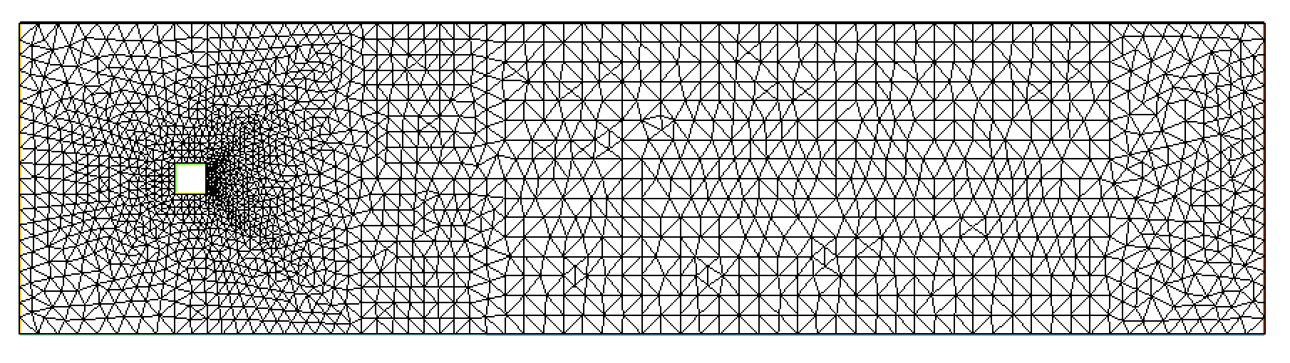
Figure 1. Flow passing an obstacle; the unstructured mesh used in the numerical experiments.

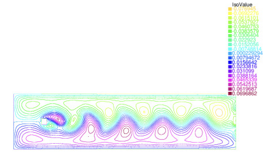
Figure 2. Streamlines for $\text{Re}=500$ at $t=45$.

We utilize the finite element method, specifically employing FreeFem++ [FreeFEM] for our simulations. For spatial discretization, we implement P2-P1 Taylor-Hood mixed finite elements, while a second-order Crank-Nicolson scheme is applied for temporal discretization (see Chapter 9 of [L08] for a comprehensive description of the scheme). The problem is computed on a Delaunay-Voronoi generated triangular mesh, which features a higher density of mesh points near the obstacle and a lower density in other areas, resulting in $17$K velocity degrees of freedom, as illustrated in Figure 1. We set $\Delta t=0.01$ and conducted the simulation from $T=0$ to $T=50$. Figure 2 shows a snapshot of the flow streamlines at $t=45$ for $\text{Re}=500$.

Energy Dissipation Rate

To numerically study the dependence of $\langle\varepsilon\rangle$ on the Reynolds number, we conducted tests with varying Reynolds numbers five times, ranging from $100$ to $2000$, by adjusting the viscosity. In Figure 3, $\varepsilon(t)$ is plotted as a function of time. As expected and observed, the pointwise values appear disordered and unpredictable. Therefore, we instead focus on the statistical (time-averaged) quantity. After averaging the energy dissipation over time, we obtained five data points, each representing $\langle\varepsilon\rangle$ corresponding to one of the Reynolds numbers. We employed Matlab’s nonlinear least squares tool to fit the data to the form $a+b\,\text{Re}^{-1}$. The initial guesses for the iterative optimization solver were set to $a_{0}=0.5$ and $b_{0}=5$. Figure 4 illustrates that the long-term average of the energy dissipation rate for the model scales as $\langle\varepsilon\rangle\sim 1+\text{Re}^{-1}$, consistent with our analysis given in Theorem 5.1.

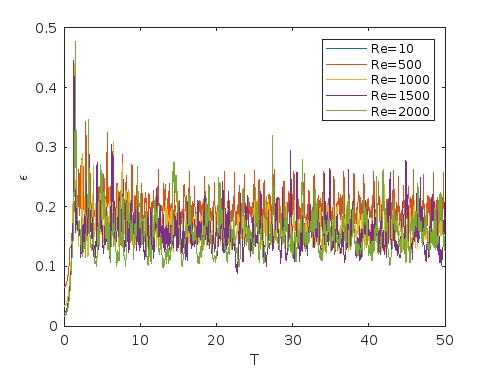
Figure 3. The energy dissipation $\varepsilon$ over time.

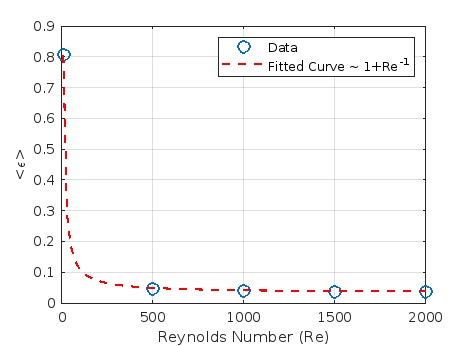
Figure 4. The time-averaged energy dissipation rate $\langle\varepsilon\rangle$ for 2D Channel flow.

7. Discussion

This paper has addressed potential issues inherent in traditional eddy viscosity turbulence models, particularly concerning excessive dissipation and parameter specification. Considering the backscatter eddy viscosity model (1.1) suggested in [RLZ19], we rigorously derived an upper bound on the energy dissipation rate per unit mass. Theorem 5.1 proves that the dissipation ratio for the backscatter eddy viscosity model (1.1) remains uniformly bounded in the infinite Reynolds number, as anticipated by heuristic scaling arguments outlined in the introduction. In this manuscript, we also address the gap in well-posedness. Despite our advancements, we acknowledge the challenges in calibrating model parameters, particularly the parameter $\beta$, where we have not identified as straightforward a mathematical or physical argument as with other parameters.

The estimate on $\langle\varepsilon\rangle$ in (5.1) is expressed in terms of controlled quantities such as $\nu$, $F$, $L$, and a derived quantity $U$. However, realizing a specific value of $U$ remains elusive, leading to a lack of a priori information regarding the dissipation rate or the intricate structure of turbulent flow for a given viscosity and applied body force. Additionally, extending our estimates of $\varepsilon$ to channel flow cases remains an open problem, which would provide valuable insights into near-wall behavior. Furthermore, broadening our analysis to two-dimensional turbulence presents an intriguing challenge, necessitating bounds on not only energy but also enstrophy dissipation rate due to the energy cascade scenario in 2D [FJMR02].

References

• [1]
• AlexakisA.DoeringC. R.Energy and enstrophy dissipation in steady-state 2d turbulencePhys. Fluids1820068085106@article{AD06, author = {Alexakis, A.}, author = {Doering, C. R.}, title = {Energy and enstrophy dissipation in steady-state 2D turbulence}, journal = {Phys. Fluids}, volume = {18}, date = {2006}, number = {8}, pages = {085106}}
• [3]
• BaldwinB.LomaxH.Thin-layer approximation and algebraic model for separated turbulent flows.AIAA 16th Aerospace Sciences Meeting1978
• [5]
• BerselliL. C.BreitD.On the existence of weak solutions for the steady baldwin- lomax model and generalizationsTechnical Report 2003.00691, arXiv2020
• [7]
• BerselliL. C.IliescuT.LaytonW. J.Mathematics of large eddy simulation of turbulent flowsScientific ComputationSpringer-Verlag, Berlin2006xviii+348
• [9]
• BerselliL. C.LewandowskiR.NguyenD. D.Rotational forms of large eddy simulation turbulence models: modeling and mathematical theoryChin. Ann. Math. Ser. B422021117–40
• [11]
• BoussinesqJ.Essai sur la theorie des eaux courantespublisher=Memoires presentes par divers savants a l’Academie des Sciences de l’Institut National de France, volume=23, date=1877,
• [13] pages=1-680,
• [14]
• [15]
• ChacónR. T.LewandowskiR.Mathematical and numerical foundations of turbulence models and applicationsModeling and Simulation in Science, Engineering and TechnologyBirkhäuser/Springer, New York2014xviii+517
• [17]
• ChowY. T.PakzadA.On the zeroth law of turbulence for the stochastically forced navier-stokes equationsDiscrete &\& Continuous Dynamical Systems - B2021@article{CP20, author = {Y. T. Chow}, author = {A. Pakzad}, title = {On the zeroth law of turbulence for the stochastically forced Navier-Stokes equations}, journal = {Discrete $\&$ Continuous Dynamical Systems - B}, date = {2021}}
• [19]
• DascaliucR.FoiasC.JollyM. S.On the asymptotic behavior of average energy and enstrophy in 3d turbulent flowsPhys. D2382009725–736@article{DFJ09, author = {R. Dascaliuc}, author = {C. Foias}, author = {M. S. Jolly}, title = {On the asymptotic behavior of average energy and enstrophy in 3D turbulent flows}, journal = {Phys. D}, volume = {238}, date = {2009}, pages = {725–736}}
• [21]
• DoeringC .R.ConstantinP.Energy dissipation in shear driven turbulencejournal=Physical review letters, volume=69, date=1992, pages=1648,
• [23]
• [24]
• DoeringC. R.FoiasC.Energy dissipation in body-forced turbulenceJ. Fluid Mech.4672002289–306
• [26]
• GronwallT. H.title=Note on the derivatives with respect to a parameter of the solutions of a system of differential equations, journal=Ann. Math. , volume=2, date=1919, pages=292 – 296,
• [28]
• [29]
• HowardL. N.Bounds on flow quantitiesjournal=Annual Review of Fluid Mechanics, volume=4, date=1972,
• [31] pages=473–494,
• [32]
• DuchonJ.RobertR.Inertial energy dissipation for weak solutions of incompressible euler and navier–stokes equationsNonlinearity132000249–255
• [34]
• FanWai. L.PakzadA.TawriK.TemamR.3D shear flows driven by lévy noise at the boundaryProbability, Uncertainty and Quantitative Risk812023@article{fan20233d, author = {Fan, Wai. L.}, author = {Pakzad, A.}, author = {Tawri, K.}, author = {Temam, R.}, title = {3D shear flows driven by Lévy noise at the boundary}, journal = {Probability, Uncertainty and Quantitative Risk}, volume = {8}, number = {1}, date = {2023}}
• [36]
• AUTHOR = Fan, W. L., AUTHOR = Jolly, M., AUTHOR = Pakzad, A., TITLE = Three-dimensional shear driven turbulence with noise at the boundary, JOURNAL = Nonlinearity, VOLUME = 34, YEAR = 2021, PAGES = 4764–4786,
• [38]
• [39]
• FoiasC.JollyM. S.ManleyO. P.RosaR.Statistical estimates for the navier-stokes equations and the kraichnan theory of 2-d fully developed turbulenceJ. Statist. Phys.10820023-4591–645
• [41]
• FrischU.TurbulenceThe legacy of A. N. KolmogorovCambridge University Press, Cambridge1995xiv+296
• [43]
• JiangN.LaytonW.Algorithms and models for turbulence not at statistical equilibriumComput. Math. Appl.712016112352–2372
• [45]
• JohnV.On large eddy simulation and variational multiscale methods in the numerical simulation of turbulent incompressible flowsAppl. Math.5120064321–353
• [47]
• HechtF.PironneauO.FreeFem++Webpage: http://www.freefem.org@article{FreeFEM, author = {Hecht, F.}, author = {Pironneau, O.}, title = {FreeFem++}, note = {Webpage: \url{http://www.freefem.org}}}
• [49]
• KolmogorovA. N.The local structure of turbulence in incompressible viscous fluid for very large reynolds numbersTranslated from the Russian by V. Levin; Turbulence and stochastic processes: Kolmogorov’s ideas 50 years onProc. Roy. Soc. London Ser. A434199118909–13
• [51]
• LadyzhenskayaO.A.Modifications of the navier–stokes equations for large gradients of the velocitiesZap. Nauˇcn. S. Leningrad. Otdel. Mat. Inst. Steklov. (LOMI)71968126–154LaytonW. J.Introduction to the numerical analysis of incompressible viscous flows6Society for Industrial and Applied Mathematics (SIAM)2008@book{L08, author = {Layton, W. J.}, title = {Introduction to the numerical analysis of incompressible viscous flows}, volume = {6}, publisher = {Society for Industrial and Applied Mathematics (SIAM)}, year = {2008}}
• [54]
• LaytonW. J.Energy dissipation in the smagorinsky model of turbulenceAppl. Math. Lett.59201656–59
• [56]
• LaytonW. J.Energy dissipation bounds for shear flows for a model in large eddy simulationMath. Comput. Modelling352002131445–1451
• [58]
• LaytonW.LewandowskiR.Analysis of an eddy viscosity model for large eddy simulation of turbulent flowsJ. Math. Fluid Mech.420024374–399
• [60]
• LundT.S.NovikovE.A.Parametrization of subgrid-scale stress by the velocity gradient tensorAnnual Research Briefs, CTRdate=1992,
• [62] pages=27–43,
• [63]
• MálekJ.NečasJ.RůžičkaM.On weak solutions to a class of non-newtonian incompressible fluids in bounded three-dimensional domains: the case $p\geq 2$2001Advances in Differential Equations63257 – 302
• [65]
• MohammadiB.PironneauO.Analysis of the $k$-epsilon turbulence modelRAM: Research in Applied MathematicsMasson, Paris; John Wiley & Sons, Ltd., Chichester1994xiv+196
• [67]
• PakzadA.Damping functions correct over-dissipation of the smagorinsky model Mathematical Methods in the Applied Sciencesvolume = 40, number = 16, issn = 1099-1476, pages = 5933–5945, year = 2017,
• [69]
• [70]
• PakzadA.Analysis of mesh effects on turbulence statisticsJournal of Mathematical Analysis and Applications475839–8602019
• [72]
• Pakzad,A.On the long time behavior of time relaxation model of fluidsPhys. DPhysica D. Nonlinear Phenomena4082020132509, 6
• [74]
• PopeS. B.Turbulent flowsCambridge University Press, Cambridge2000xxxiv+771
• [76]
• RichardsonL. F.Weather prediction by numerical process,Cambridge, UK: Cambridge Univ. Pressdate=1922,
• [78]
• [79]
• RivlinR.S.The relation between the flow of non-newtonian fluids and turbulent newtonian fluidsQuarterly of Appl. Math151957
Conversion to HTML had a Fatal error and exited abruptly. This document may be truncated or damaged.