Exploiting Dynamic Sparsity for Near-Field Spatial Non-Stationary XL-MIMO Channel Tracking

Abstract

This work considers a spatial non-stationary channel tracking problem in broadband extremely large-scale multiple-input-multiple-output (XL-MIMO) systems. In the case of spatial non-stationary, each scatterer has a certain visibility region (VR) over antennas and power change may occur among visible antennas. Concentrating on the temporal correlation of XL-MIMO channels, we design a three-layer Markov prior model and hierarchical two-dimensional (2D) Markov model to exploit the dynamic sparsity of sparse channel vectors and VRs, respectively. Then, we formulate the channel tracking problem as a bilinear measurement process, and a novel dynamic alternating maximum a posteriori (DA-MAP) framework is developed to solve the problem. The DA-MAP contains four basic modules: channel estimation module, VR detection module, grid update module, and temporal correlated module. Specifically, the first module is an inverse-free variational Bayesian inference (IF-VBI) estimator that avoids computational intensive matrix inverse each iteration; the second module is a turbo compressive sensing (Turbo-CS) algorithm that only needs small-scale matrix operations in a parallel fashion; the third module refines the polar-delay domain grid; and the fourth module can process the temporal prior information to ensure high-efficiency channel tracking. Simulations show that the proposed method can achieve a significant channel tracking performance while achieving low computational overhead.

I Introduction

Extremely large-scale multiple-input-multiple-output (XL-MIMO) is a promising technology with many applications for future 6G communications [1]. With an even larger number of antennas at the base station (BS) compared to traditional massive MIMO systems, XL-MIMO can offer higher data rates, improved spectral efficiency, and enhanced system reliability [2]. To reap the benefits of XL-MIMO, it is essential to track channel state information (CSI) accurately over a time-varying wireless channel [3, 4, 5, 6].

There are a number of characteristics of XL-MIMO channels that distinguish it from conventional MIMO channels [7, 8, 9, 10]. First of all, the effect of near-field propagation is obvious. Due to the large antenna aperture of XL-MIMO, the near-field region (Rayleigh region) of the array is also large [7]. The array experiences a spherical wave within the Rayleigh region, and the resulting steering vector accounts for both angle and distance parameters of last-hop scatterers [8]. Secondly, the spatial non-stationary effect is likely to exist. Spatial non-stationary means that each scatterer can only see a subset of antennas, i.e., it has a certain visibility region (VR) over the antennas [9]. Furthermore, the measurements in [10] revealed that power change among visible antenna elements may occur in some channel paths. In this case, VR needs to be modeled as a continuous variable instead of a 0/1 discrete variable, which makes the VR issue more challenging. Thirdly, the XL-MIMO channel varies quickly over time. Fortunately, there is a temporal correlation among XL-MIMO channels. Specifically, although the channel varies quickly over time, the scattering environment, which consists of the angle, distance, and VR of scatterers, changes quite slowly in adjacent frames. By exploiting this temporal correlation, the channel tracking performance is expected to be enhanced significantly. Some related works on how to estimate and track spatial non-stationary channels are summarized below.

Spatial non-stationary channel estimation: There are mainly three types of VR modeling methods, and different VR modeling methods lead to different algorithm designs for channel estimation. The first one is called the sub-array-level 0/1 modeling. In this model, the large-scale array are divided into a number of small-scale sub-arrays, and each sub-channel corresponding to each sub-array is assumed to be spatial stationary. Based on the sub-array grouping, binary vectors are used to model the VR of scatterers and sub-arrays. Such a modeling method was firstly introduced in [11], and a sub-array-wise orthogonal matching pursuit (OMP) algorithm was designed for channel estimation. Inspired by this, many sub-array-wise methods were developed for addressing the spatial non-stationary issue [12, 13, 14]. Generally speaking, the sub-array-wise methods first estimate each spatial stationary sub-channel independently, and then combine the obtained sub-channels into the whole channel. Apparently, they work poorly in the low SNR regions since the correlation among sub-channels is ignored. Moreover, the spatial stationary of each sub-array cannot be ensured in practice. To overcome this drawback, the antenna-level 0/1 modeling for VR was used in [15, 16]. This model considers the VR of each antenna without sub-array grouping, and the visible antennas are concentrated on a few clusters. The work in [15] used a Markov chain to capture the clustered sparsity of the VR and proposed a turbo orthogonal approximate message passing (Turbo-OAMP) algorithm. However, such an algorithm directly processes the received signal in the space domain, which cannot exploit the polar-domain sparsity of XL-MIMO channels [8]. In [16], the authors developed a two-stage method to exploit the sparsity of channels. But it was only confined to the single-path scenario. For more general multi-path scenario, [17] proposed a novel alternating maximum a posteriori (MAP) framework to achieve joint VR detection and channel estimation. Recently, power change among visible antennas was observed in [10]. A more accurate VR modeling method was proposed, in which the VR was no longer based on the 0/1 assumption but treated as a continuous variable. Motivated by this, [18] developed a robust fast sparse Bayesian learning (RFSBL) algorithm to estimate the continuous VRs.

Multi-frame channel tracking: The above works focus on channel estimation for each frame separately, while the temporal correlation among multiple frames is not considered. To the best of our knowledge, there is still a lack of research on spatial non-stationary channel tracking. Nevertheless, some early attempts at massive MIMO channel tracking inspire us a lot. In particular, [3] formulated the multi-frame tracking problem as a dynamic compressive sensing (CS) problem, and an approximate message passing (AMP) algorithm is used to solve the problem. The work in [4] used a Markov chain to model the temporal correlation of channels and designed a Turbo-OAMP algorithm to track the dynamic channels with the Markov prior. [5, 6] considered practical system imperfections and tracked the dynamic channels and system imperfections jointly. Although these methods have elaborated on how to exploit the dynamic sparsity of spatial stationary channels, they cannot be directly applied to the case of spatial non-stationary channels. The reasons are two folds: 1) how to exploit the temporal correlation of VRs is still known; 2) these algorithms are used to deal with the linear measurement process, while the considered spatial non-stationary channel tracking problem is a bilinear measurement process.

In this work, we consider a non-stationary channel tracking problem in a broadband multi-carrier XL-MIMO system under a hybrid beamforming (HBF) architecture. Based on the literature review, there are some challenges in the considered problem. Firstly, it is important to design a proper prior model to capture the temporal correlation of both sparse channel vectors and continuous VRs. Secondly, the considered problem is a bilinear measurement process, and thus a new algorithmic framework needs to be developed to solve the problem. Thirdly, due to the large number of antennas and sub-carriers, the dimension of XL-MIMO channels is extremely high. Therefore, low computational overhead is also essential while acquiring CSI accurately. This paper aims to address these challenges and the main contributions are summarized as follows.

• Encoded sub-array HBF architecture: The received signals of antennas are mixed together due to HBF, which makes it difficult to decouple the individual received signal at each antenna for further VR detection. Inspired by [14], a more generalized signal extraction scheme is developed based on an encoded sub-array HBF architecture.

• Prior design for the dynamic sparsity: A three-layer Markov prior model is designed to capture the dynamic sparsity of the polar-delay domain channel vectors in multiple frames. Besides, we introduce a hierarchical two-dimensional (2D) Markov model to exploit the clustered sparsity of VRs over antennas and correlation over time.

• Dynamic alternating MAP (DA-MAP): A novel DA-MAP framework is proposed to deal with the bilinear measurement process. The DA-MAP framework consists of four basic modules: channel estimation module, VR detection module, grid update module, and temporal correlated module. Specifically, the first module is used to estimate the polar-delay domain channel vectors, while the second module is employed to recover continuous VRs. Furthermore, the third module refines the polar-delay domain grid, and the fourth module handles the temporal prior information passed from the previous frame to the current frame. For each frame, the channel estimation module, VR detection module, and grid update module work alternatively to perform high-accuracy spatial non-stationary channel estimation. Among multiple frames, the temporal correlated module exploits the temporal correlation to achieve robust channel tracking.

• Low-complexity designs: Low-complexity designs are introduced to reduce the computational complexity of the DA-MAP framework. For the channel estimation module, we use an inverse-free variational Bayesian inference (IF-VBI) estimator [17, 19] that avoids the computational intensive matrix inverse operation. Besides, the turbo compressive sensing (Turbo-CS) algorithm [20] is designed as the VR detection module, which only needs small-scale matrix operations in a parallel fashion by resorting to polar-delay domain filtering. Furthermore, exploiting information from the previous frame as the prior for the next one, the iteration number of the DA-MAP is reduced significantly during channel tracking. As a result, the DA-MAP obtains an excellent channel tracking performance while achieving low computational overhead.

The rest of the paper proceeds as follows. Section II presents the channel model and encoded sub-array HBF architecture. Section III formulates the considered problem into a bilinear measurement process. Section IV elaborates on the DA-MAP framework. The simulations results are shown in Section V. Finally, the paper is concluded in Section VI.

Notations: Lowercase and uppercase bold letterers denote vectors and matrices, respectively. Let $\left(\cdot\right)^{-1}$, $\left(\cdot\right)^{T}$, $\left(\cdot\right)^{H}$, $\left\langle\cdot\right\rangle$, $\left\|\cdot\right\|$, $\textrm{vec}\left(\cdot\right)$, and $\textrm{diag}\left(\cdot\right)$ represent the inverse, transpose, conjugate transpose, expectation, $\ell_{2}\textrm{-norm}$, vectorization, and diagonalization operations, respectively. $\otimes$ is the Kronecker product operator and $\odot$ means the Hadamard product operator. $\Re\left\{\cdot\right\}$ and $\Im\left\{\cdot\right\}$ denote the real and imaginary part of the complex argument, respectively. $\mathbf{I}_{N}$ is the $N\times N$ dimensional identity matrix and $\mathbf{1}_{M\times N}$ is the $M\times N$ dimensional all-one matrix. For a set $\mathbf{\Omega}$ with its cardinal number denoted by $\left|\mathbf{\Omega}\right|$, $\boldsymbol{x}\triangleq\left[x_{n}\right]_{n\in\mathbf{\Omega}}\in\mathbb{C}^{\left|\mathbf{\Omega}\right|\times 1}$ is a vector composed of elements indexed by $\mathbf{\Omega}$. $\mathcal{CN}\left(\boldsymbol{x};\boldsymbol{\mu},\mathbf{\Sigma}\right)$ denotes the complex Gaussian distribution with mean $\boldsymbol{\mu}$ and covariance $\mathbf{\Sigma}$. $\textrm{Ga}\left(x;a,b\right)$ denotes the Gamma distribution with shape parameter $a$ and rate parameter $b$.

II System Model

II-A Broadband XL-MIMO System under Hybrid Beamforming

Consider an uplink time division duplexing (TDD) based broadband XL-MIMO system, where a BS serves single-antenna users, as illustrated in Fig. 1. The BS is equipped with a half-wavelength uniform linear array (ULA) of $M$ antennas and a sub-array HBF architecture with $N_{\textrm{RF}}\ll M$ RF chains. Assume that $N_{\textrm{RF}}$ is divisible by $M$ and partition the ULA into $N_{\textrm{RF}}$ sub-arrays uniformly, with each sub-array containing $M_{\textrm{sub}}=\frac{M}{N_{\textrm{RF}}}$ antennas. All the antennas in the same sub-array is only connected with one RF chain, which can effectively reduce hardware complexity [21]. Each single-antenna user is allocated with a subset of $N$ subcarriers for channel estimation. Since different users are assigned with orthogonal frequency resources during channel estimation [22], we shall focus on a certain user. The center frequency is $f_{c}$, the subcarrier interval is $f_{0}$, and the wavelength is $\lambda_{c}=\frac{c}{f_{c}}$, where $c$ is the speed of light.

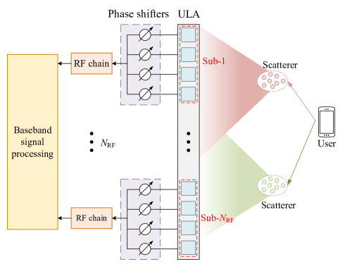
Figure 1: Illustration of the spatial non-stationary XL-MIMO channel and the sub-array HBF architecture.

In the $t\textrm{-th}$ frame, the user transmits a pilot sequence of length $P$ to the BS for channel estimation. Then, the received signal of the $p\textrm{-th}$ pilot symbol on the $n\textrm{-th}$ subcarrier, denoted by $\boldsymbol{y}_{p}^{\left(t\right)}\left[n\right]\in\mathbb{C}^{N_{\textrm{RF}}\times 1}$, is expressed as

$$\boldsymbol{y}_{p}^{\left(t\right)}\left[n\right]=\mathbf{W}_{p}^{\left(t\right)}\boldsymbol{h}^{\left(t\right)}\left[n\right]v_{p}^{\left(t\right)}\left[n\right]+\mathbf{W}_{p}^{\left(t\right)}\boldsymbol{z}_{p}^{\left(t\right)}\left[n\right],$$ (1)

where $\boldsymbol{h}^{\left(t\right)}\left[n\right]\in\mathbb{C}^{M\times 1}$ is the channel response vector that is assumed to stay unchanged within each frame, $v_{p}^{\left(t\right)}\left[n\right]\in\mathbb{C}$ is the pilot symbol with unit power, and $\boldsymbol{z}_{p}^{\left(t\right)}\left[n\right]\in\mathbb{C}^{M\times 1}$ is the additive white Gaussian noise (AWGN) with variance $1/\gamma_{z}^{\left(t\right)}$. The $\mathbf{W}_{p}^{\left(t\right)}\in\mathbb{C}^{N_{\textrm{RF}}\times M}$ in (1) is the constant amplitude analog phase shifter matrix, which is defined as

$$\mathbf{W}_{p}^{\left(t\right)}\triangleq\textrm{BlockDiag}\left(\left(\boldsymbol{w}_{p,1}^{\left(t\right)}\right)^{T},\ldots,\left(\boldsymbol{w}_{p,N_{\textrm{RF}}}^{\left(t\right)}\right)^{T}\right).$$ (2)

where $\textrm{BlockDiag}\left(\cdot\right)$ denotes the block diagonal operator, and the analog phase shifter vector for the $k\textrm{-th}$ sub-array is $\boldsymbol{w}_{p,k}^{\left(t\right)}\triangleq\left[e^{j\varphi_{p,k,1}^{\left(t\right)}},\ldots,e^{j\varphi_{p,k,M_{\textrm{sub}}}^{\left(t\right)}}\right]^{T}\in\mathbb{C}^{M_{\textrm{sub}}\times 1}$ with $\varphi_{p,k,m}^{\left(t\right)}\in\left[0,2\pi\right]$ for $m=1,\ldots,M_{\textrm{sub}}$.

Due to the near-field propagation and spatial non-stationary, the XL-MIMO channel $\boldsymbol{h}^{\left(t\right)}\left[n\right]$ is quite different from the traditional massive MIMO channel. The modeling of $\boldsymbol{h}^{\left(t\right)}\left[n\right]$ is discussed next.

II-B Spatial Non-stationary Channel Model

In a high-frequency XL-MIMO system, the Rayleigh distance is hundreds or even thousands of meters [7, 1]. In this case, near-field propagation cannot be ignored, and the steering vector is related to both the angle and distance parameters of scatterers. Without loss of generality, we set the center of the ULA as the origin of the coordinate system. Let $\delta_{m}=m-\frac{M+1}{2}$ represent the relative index of the $m\textrm{-th}$ antenna. Then the coordinates of the $m\textrm{-th}$ antenna can be expressed as $\boldsymbol{p}_{m}=\left[\delta_{m}d,0\right]^{T}$, where $d=\frac{\lambda_{c}}{2}$ is the antenna spacing.

Consider a scatterer with angle of arrival (AoA) $\theta$ and distance $r$, whose coordinates is $\boldsymbol{p}=\left[r\cos\theta,r\sin\theta\right]^{T}$. The distance between the scatterer and the $m\textrm{-th}$ antenna can be derived as

$$r_{m}=\left\|\boldsymbol{p}-\boldsymbol{p}_{m}\right\|=\sqrt{r^{2}+\delta_{m}^{2}d^{2}-2r\delta_{m}d\cos\theta}.$$ (3)

Based on the uniform spherical wave (USW) model [23], the steering vector at the BS is given by

$$\boldsymbol{a}\left(\theta,r\right)=\frac{1}{\sqrt{M}}\left[e^{-j\frac{2\pi}{\lambda_{c}}\left(r_{1}-r\right)},\ldots,e^{-j\frac{2\pi}{\lambda_{c}}\left(r_{M}-r\right)}\right]^{T}.$$ (4)

Since the form in (4) is quite complicated, we introduce the Fresnel approximation to approximate the distance $r_{m}$ [24],

$$r_{m}\approx r-\delta_{m}d\vartheta+\frac{\delta_{m}^{2}d^{2}}{2r}\left(1-\vartheta^{2}\right),$$ (5)

where $\vartheta\triangleq\cos\theta$. The above Fresnel approximation has been verified to be accurate enough and widely used in near-field channel modeling [7, 8, 25]. Submitting (5) into (4), the simplified steering vector based on the Fresnel approximation is obtained as

$$\left[\boldsymbol{a}\left(\vartheta,r\right)\right]_{m}=\frac{1}{\sqrt{M}}e^{-j\frac{2\pi}{\lambda_{c}}\left(-\delta_{m}d\vartheta+\frac{\delta_{m}^{2}d^{2}}{2r}\left(1-\vartheta^{2}\right)\right)},$$ (6)

where $\left[\boldsymbol{a}\left(\vartheta,r\right)\right]_{m}$ is the $m\textrm{-th}$ element of $\boldsymbol{a}\left(\vartheta,r\right)$.

Besides, the spatial non-stationary effect means that each scatterer has a certain VR over antennas. Let $L^{\left(t\right)}$ denote the number of channel paths in $\boldsymbol{h}^{\left(t\right)}\left[n\right]$. Define $\boldsymbol{u}_{l}^{\left(t\right)}\triangleq\Bigl{[}u_{l,1}^{\left(t\right)},\ldots,u_{l,M}^{\left(t\right)}\Bigr{]}^{T}\in\mathbb{C}^{M\times 1}$ as the VR vector of scatterer $l$ in the $t\textrm{-th}$ frame, where $u_{l,m}^{\left(t\right)}\geq 0$ represents the received power of the $l\textrm{-th}$ path on the $m\textrm{-th}$ antenna with $u_{l,m}^{\left(t\right)}=0$ indicating the $m\textrm{-th}$ antenna is invisible to scatterer $l$ [10]. Consequently, the channel vector is modeled as

$$\boldsymbol{h}^{\left(t\right)}\left[n\right]=\sum_{l=1}^{L^{\left(t\right)}}x_{l}^{\left(t\right)}e^{-j2\pi nf_{0}\tau_{l}^{\left(t\right)}}\boldsymbol{a}\left(\vartheta_{l}^{\left(t\right)},r_{l}^{\left(t\right)}\right)\odot\boldsymbol{u}_{l}^{\left(t\right)},$$ (7)

where $x_{l}^{\left(t\right)}$, $\tau_{l}^{\left(t\right)}$, $\vartheta_{l}^{\left(t\right)}$, and $r_{l}^{\left(t\right)}$ represent the complex channel gain, delay, angle, and distance of the $l\textrm{-th}$ path.

II-C Encoded Sub-array HBF Architecture

From (1), we notice that the received signal of each RF chain is a mixture of the received signal of antennas in its associated sub-array. In [14], a signal extraction scheme is developed when a fully connected HBF architecture is used for $\mathbf{W}_{p}^{\left(t\right)}$. However, the number of antennas is confined to $M=2^{i},i\in\mathbb{N}+$ and the number of pilots is confined to $P=N_{P}M,N_{P}\in\mathbb{N}+$. Moreover, it needs at least $P=M$ pilot observations to decouple the signals from each antenna, which leads to a large pilot overhead and is unacceptable for practical XL-MIMO systems. To overcome these drawbacks, we make use of the block diagonal structure in (2) and propose a more generalized signal extraction scheme based on an encoded sub-array HBF architecture.

In particular, the received signal of the $k\textrm{-th}$ RF chain can be expressed as

$$y_{p,k}^{\left(t\right)}\left[n\right]=\left(\boldsymbol{w}_{p,k}^{\left(t\right)}\right)^{T}\left(\boldsymbol{h}_{\textrm{sub-}k}^{\left(t\right)}\left[n\right]v_{p}^{\left(t\right)}\left[n\right]+\boldsymbol{z}_{p,\textrm{sub-}k}^{\left(t\right)}\left[n\right]\right),$$ (8)

where $\boldsymbol{h}_{\textrm{sub-}k}^{\left(t\right)}\left[n\right]\triangleq\left[h_{m}^{\left(t\right)}\left[n\right]\right]_{m\in\mathbf{\Psi}_{k}}$ and $\boldsymbol{z}_{p,\textrm{sub-}k}^{\left(t\right)}\left[n\right]\triangleq\left[z_{p,m}^{\left(t\right)}\left[n\right]\right]_{m\in\mathbf{\Psi}_{k}}$ denote the channel vector and noise vector corresponding to the $k\textrm{-th}$ sub-array, respectively, and $\mathbf{\Psi}_{k}\triangleq\left\{m+\left(k-1\right)M_{\textrm{sub}}\mid m=1,\ldots,M_{\textrm{sub}}\right\}$ is the index set of antennas in the $k\textrm{-th}$ sub-array. To simplify the notation, we temporarily omit the indices of subcarriers and frames. Then, (8) can be rewritten into

$$y_{p,k}=\left(\boldsymbol{w}_{p,k}\right)^{T}\left(\boldsymbol{h}_{\textrm{sub-}k}v_{p}+\boldsymbol{z}_{p,\textrm{sub-}k}\right),\forall p.$$ (9)

The goal is to acquire the individual received signal at $M_{\textrm{sub}}$ antennas from $P$ linear mixture measurements of (9), where $P\geqslant M_{\textrm{sub}}$ is a necessary condition.

Focusing on the case of $P\geqslant M_{\textrm{sub}}$, we encode the phase shifter vectors as

$$\left[\boldsymbol{w}_{1,k},\ldots,\boldsymbol{w}_{P,k}\right]^{T}=\mathbf{D}_{P},$$ (10)

where $\mathbf{D}_{P}\in\mathbb{C}^{P\times M_{\textrm{sub}}}$ consists of the first $M_{\textrm{sub}}$ columns of the $P$-dimensional discrete Fourier transform (DFT) matrix such that $\mathbf{D}_{P}^{H}\mathbf{D}_{P}=P\mathbf{I}_{M_{\textrm{sub}}}$. Then, the received signal of each antenna can be decoupled as

$$\tilde{\boldsymbol{y}}_{\textrm{sub-}k} =\frac{1}{P}\mathbf{D}_{P}^{H}\left[\frac{y_{1,k}}{v_{1}},\ldots,\frac{y_{P,k}}{v_{P}}\right]^{T},$$

$$=\boldsymbol{h}_{\textrm{sub-}k}+\tilde{\boldsymbol{z}}_{\textrm{sub-}k},$$ (11)

where $\tilde{\boldsymbol{z}}_{\textrm{sub-}k}\in\mathbb{C}^{M_{\textrm{sub}}\times 1}$ is the equivalent noise vector with variance $\gamma^{\left(t\right)}=\frac{P}{M_{\textrm{sub}}\gamma_{z}^{\left(t\right)}}$.

Stacking the decoupled signals of all RF chains into a single vector gives

$$\tilde{\boldsymbol{y}}^{\left(t\right)}\left[n\right]=\boldsymbol{h}^{\left(t\right)}\left[n\right]+\tilde{\boldsymbol{z}}^{\left(t\right)}\left[n\right],$$ (12)

where

$$\tilde{\boldsymbol{y}}^{\left(t\right)}\left[n\right] \triangleq\left[\left(\tilde{\boldsymbol{y}}_{\textrm{sub-}1}^{\left(t\right)}\left[n\right]\right)^{T},\ldots,\left(\tilde{\boldsymbol{y}}_{\textrm{sub-}N_{\textrm{RF}}}^{\left(t\right)}\left[n\right]\right)^{T}\right]^{T}\in\mathbb{C}^{M\times 1},$$

$$\tilde{\boldsymbol{z}}^{\left(t\right)}\left[n\right] \triangleq\left[\left(\tilde{\boldsymbol{z}}_{\textrm{sub-}1}^{\left(t\right)}\left[n\right]\right)^{T},\ldots,\left(\tilde{\boldsymbol{z}}_{\textrm{sub-}N_{\textrm{RF}}}^{\left(t\right)}\left[n\right]\right)^{T}\right]^{T}\in\mathbb{C}^{M\times 1}.$$

Further stacking $\tilde{\boldsymbol{y}}^{\left(t\right)}\left[n\right]$ for all $N$ subcarriers, we obtain

$$\tilde{\mathbf{Y}}^{\left(t\right)}=\mathbf{H}^{\left(t\right)}+\tilde{\mathbf{Z}}^{\left(t\right)},$$ (13)

where $\mathbf{H}^{\left(t\right)}\triangleq\left[\left(\boldsymbol{h}^{\left(t\right)}\left[1\right]\right)^{T};\ldots;\left(\boldsymbol{h}^{\left(t\right)}\left[N\right]\right)^{T}\right]\in\mathbb{C}^{N\times M}$ is the frequency-antenna domain channel matrix, and $\tilde{\mathbf{Y}}^{\left(t\right)}$ and $\tilde{\mathbf{Z}}^{\left(t\right)}$ are defined similarly. Vectorization of $\tilde{\mathbf{Y}}^{\left(t\right)}$ yields

$$\tilde{\boldsymbol{y}}^{\left(t\right)}=\boldsymbol{h}^{\left(t\right)}+\tilde{\boldsymbol{z}}^{\left(t\right)},$$ (14)

where $\tilde{\boldsymbol{y}}^{\left(t\right)}=\textrm{vec}\left(\tilde{\mathbf{Y}}^{\left(t\right)}\right)$, $\boldsymbol{h}^{\left(t\right)}=\textrm{vec}\left(\mathbf{H}^{\left(t\right)}\right)$, and $\tilde{\boldsymbol{z}}^{\left(t\right)}=\textrm{vec}\left(\tilde{\mathbf{Z}}^{\left(t\right)}\right)$.

III Prior Design for the Dynamic Sparsity

III-A Polar-delay Domain Sparse Representation

Due to the small number of paths constituting the channel, grid-based sparse representation of wireless channels is commonly used [26]. Recently, the work in [8] studied the sparse characteristic of single-carrier near-field channels and proposed a polar-domain sparse representation. However, with multi-carrier and spatial non-stationary, the sparse representation is quite different.

We first introduce a polar-domain grid of $Q_{1}$ points, where the sampling points $\left\{\bar{\vartheta}_{q_{1}},\bar{r}_{q_{1}}\right\}_{q_{1}=1}^{Q_{1}}$ are generated using Algorithm 1 in [8]. Then, we introduce a delay-domain grid of $Q_{2}$ points, such that the sampling delay points $\left\{\bar{\tau}_{q_{2}}\right\}_{q_{2}=1}^{Q_{2}}$ are uniformly within $\left[0,\tau_{\textrm{max}}\right]$, where $\tau_{\textrm{max}}$ is the delay spread. Based on these, the initial polar-delay domain grid is defined as

$$\bar{\mathbf{\Xi}}\triangleq \left[\left[\bar{\vartheta}_{1},\bar{r}_{1},\bar{\tau}_{1}\right];\ldots;\left[\bar{\vartheta}_{1},\bar{r}_{1},\bar{\tau}_{Q_{2}}\right];\ldots\right.$$

$$\left[\bar{\vartheta}_{q_{1}},\bar{r}_{q_{1}},\bar{\tau}_{1}\right];\ldots;\left[\bar{\vartheta}_{q_{1}},\bar{r}_{q_{1}},\bar{\tau}_{Q_{2}}\right];\ldots$$

$$\left.\left[\bar{\vartheta}_{Q_{1}},\bar{r}_{Q_{1}},\bar{\tau}_{1}\right];\ldots;\left[\bar{\vartheta}_{Q_{1}},\bar{r}_{Q_{1}},\bar{\tau}_{Q_{2}}\right]\right].$$ (15)

It is obvious that the fixed grid $\bar{\mathbf{\Xi}}$ of $Q=Q_{1}\times Q_{2}$ points usually cannot cover the true angle, distance, and delay parameters of scatterers. And thus, the channel estimation performance is limited by the grid interval [27]. To achieve high-accuracy channel tracking, we introduce a dynamic polar-delay domain grid in each frame, denoted by $\mathbf{\Xi}^{\left(t\right)}\triangleq\left[\boldsymbol{\vartheta}^{\left(t\right)},\boldsymbol{r}^{\left(t\right)},\boldsymbol{\tau}^{\left(t\right)}\right],\forall t$, where $\boldsymbol{\vartheta}^{\left(t\right)}\triangleq\left[\vartheta_{1}^{\left(t\right)},\ldots,\vartheta_{Q}^{\left(t\right)}\right]^{T}$, $\boldsymbol{r}^{\left(t\right)}\triangleq\left[r_{1}^{\left(t\right)},\ldots,r_{Q}^{\left(t\right)}\right]^{T}$, and $\boldsymbol{\tau}^{\left(t\right)}\triangleq\left[\tau_{1}^{\left(t\right)},\ldots,\tau_{Q}^{\left(t\right)}\right]^{T}$ represent the angle, distance, and delay grid vectors, respectively, at time $t$. We can initialize the dynamic grid by $\mathbf{\Xi}^{\left(0\right)}=\bar{\mathbf{\Xi}}$.

Then, the polar-delay domain basis is obtained as

$$\mathbf{B}\left(\mathbf{\Xi}^{\left(t\right)}\right)\triangleq\left[\boldsymbol{b}\left(\vartheta_{1}^{\left(t\right)},r_{1}^{\left(t\right)},\tau_{1}^{\left(t\right)}\right),\ldots,\boldsymbol{b}\left(\vartheta_{Q}^{\left(t\right)},r_{Q}^{\left(t\right)},\tau_{Q}^{\left(t\right)}\right)\right],$$ (16)

with $\boldsymbol{b}\left(\vartheta_{q}^{\left(t\right)},r_{q}^{\left(t\right)},\tau_{q}^{\left(t\right)}\right)\in\mathbb{C}^{MN\times 1},\forall q$ given by

$$\boldsymbol{b}\left(\vartheta_{q}^{\left(t\right)},r_{q}^{\left(t\right)},\tau_{q}^{\left(t\right)}\right)=\boldsymbol{a}\left(\vartheta_{q}^{\left(t\right)},r_{q}^{\left(t\right)}\right)\otimes\boldsymbol{d}\left(\tau_{q}^{\left(t\right)}\right),$$ (17)

where $\boldsymbol{d}\left(\tau\right)\triangleq\left[e^{-j2\pi f_{0}\tau},\ldots,e^{-j2\pi Nf_{0}\tau}\right]^{T}\in\mathbb{C}^{N\times 1}$ represents the delay response vector.

Furthermore, we introduce a VR dictionary corresponding to the polar-delay domain basis, denoted by $\mathbf{U}^{\left(t\right)}=\left[\boldsymbol{u}_{1}^{\left(t\right)},\ldots,\boldsymbol{u}_{Q}^{\left(t\right)}\right]\in\mathbb{C}^{M\times Q}$, where $\boldsymbol{u}_{q}^{\left(t\right)}$ represents the VR of the scatterer lying around the $q\textrm{-th}$ polar-delay domain grid point. Then, the sparse representation of the channel vector in (14) can be obtained as

$$\boldsymbol{h}^{\left(t\right)}=\underbrace{\left[\mathbf{B}\left(\mathbf{\Xi}^{\left(t\right)}\right)\odot\left(\mathbf{U}^{\left(t\right)}\otimes\boldsymbol{1}_{N\times 1}\right)\right]}_{\mathbf{F}\left(\mathbf{\Xi}^{\left(t\right)},\mathbf{U}^{\left(t\right)}\right)}\boldsymbol{x}^{\left(t\right)},$$ (18)

where $\boldsymbol{x}^{\left(t\right)}\in\mathbb{C}^{Q\times 1}$ is called the polar-delay domain sparse channel vector and $\mathbf{F}\left(\mathbf{\Xi}^{\left(t\right)},\mathbf{U}^{\left(t\right)}\right)$ is the transform matrix. The $q\textrm{-th}$ element of $\boldsymbol{x}^{\left(t\right)}$, denoted by $x_{q}^{\left(t\right)}$, represents the complex gain of the channel path with angle $\vartheta_{q}^{\left(t\right)}$, distance $r_{q}^{\left(t\right)}$, and delay $\tau_{q}^{\left(t\right)}$.

The sparse representation in (18) is a generalization of the model in [8]. In particular, when $\mathbf{U}^{\left(t\right)}=\boldsymbol{1}_{M\times Q}$, (18) gives the sparse representation of multi-carrier spatial stationary channels. Further with $N=1$, (18) reduced to the model in [8].

III-B Sparse Prior Model

The sparse prior model is essential to capture the specific sparse structure and perform sparse signal recovery. In this subsection, we first introduce a three-layer Markov prior model to capture the dynamic sparsity of the polar-delay domain sparse channel vectors. Then, a hierarchical 2D Markov model is designed to exploit the clustered sparsity of VRs over antennas and correlation over time.

III-B1 Three-layer Markov Prior Model for Channels

The three-layer Markov prior model is used to describe the sparse structure of $\boldsymbol{x}^{\left(t\right)},\forall t$, as illustrated in Fig. 2. Define $\boldsymbol{\rho}^{\left(t\right)}\triangleq\left[\rho_{1}^{\left(t\right)},\ldots,\rho_{Q}^{\left(t\right)}\right]^{T}$ and $\boldsymbol{s}^{\left(t\right)}\triangleq\left[s_{1}^{\left(t\right)},\ldots,s_{Q}^{\left(t\right)}\right]^{T}$ as the precision and support vector of $\boldsymbol{x}^{\left(t\right)}$, respectively, where $1/\rho_{q}^{\left(t\right)}$ is the variance of $x_{q}^{\left(t\right)}$ and $s_{q}^{\left(t\right)}\in\left\{0,1\right\}$ indicates $x_{q}^{\left(t\right)}$ is a non-zero element or not. Denote the time series $\left\{\boldsymbol{x}^{\left(1\right)},...,\boldsymbol{x}^{\left(T\right)}\right\}$ as $\boldsymbol{x}^{\left(1:T\right)}$ (same for $\boldsymbol{\rho}^{\left(1:T\right)}$ and $\boldsymbol{s}^{\left(1:T\right)}$), where $T$ is the total number of frames. The joint distribution of $\boldsymbol{x}^{\left(1:T\right)}$, $\boldsymbol{\rho}^{\left(1:T\right)}$, and $\boldsymbol{s}^{\left(1:T\right)}$ is expressed as

$$p\left(\boldsymbol{x}^{\left(1:T\right)},\boldsymbol{\rho}^{\left(1:T\right)},\boldsymbol{s}^{\left(1:T\right)}\right)$$

$$= \underbrace{p\left(\boldsymbol{s}^{\left(1:T\right)}\right)}_{\textrm{Support}}\prod_{t=1}^{T}\underbrace{p\left(\boldsymbol{\rho}^{\left(t\right)}\mid\boldsymbol{s}^{\left(t\right)}\right)}_{\textrm{Precision}}\prod_{t=1}^{T}\underbrace{p\left(\boldsymbol{x}^{\left(t\right)}\mid\boldsymbol{\rho}^{\left(t\right)}\right)}_{\textrm{Sparse\ signal}}.$$ (19)

Since the scattering environment changes slowly over time, there exists a strong temporal correlation among support vectors. To be more specific, if $s_{q}^{\left(t-1\right)}=1$, then $s_{q}^{\left(t\right)}$ is also equal to 1 with high probability. Therefore, we use a Markov chain to model support vectors,

$$p\left(\boldsymbol{s}^{\left(1:T\right)}\right)=\prod_{q=1}^{Q}\left(p\left(s_{q}^{\left(1\right)}\right)\prod_{t=2}^{T}p\left(s_{q}^{\left(t\right)}\mid s_{q}^{\left(t-1\right)}\right)\right),$$ (20)

with the transition probability given by

$$p_{01}^{x} =p\left(s_{q}^{\left(t\right)}=1\mid s_{q}^{\left(t-1\right)}=0\right),$$ (21a)

$$p_{10}^{x} =p\left(s_{q}^{\left(t\right)}=0\mid s_{q}^{\left(t-1\right)}=1\right).$$ (21b)

The value of the transition probability reflects the strength of temporal correlation. Specifically, small $p_{01}^{x}$ and $p_{10}^{x}$ imply a strong temporal correlation, while large $p_{01}^{x}$ and $p_{10}^{x}$ imply the opposite. The steady-state distribution of the Markov chain is used as the initial distribution, i.e., $p\left(s_{q}^{\left(1\right)}=1\right)=\frac{p_{01}^{x}}{p_{01}^{x}+p_{10}^{x}}$.

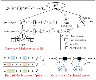
Figure 2: Three-layer Markov prior model to exploit the dynamic sparsity of polar-delay domain channels.

The precision vector is modeled as a Bernoulli-Gamma distribution, which is given by

$$p\left(\boldsymbol{\rho}^{\left(t\right)}\mid\boldsymbol{s}^{\left(t\right)}\right)=\prod_{q=1}^{Q}\textrm{Ga}\left(\rho_{q}^{\left(t\right)};a,b\right)^{s_{q}^{\left(t\right)}}\textrm{Ga}\left(\rho_{q}^{\left(t\right)};\bar{a},\bar{b}\right)^{1-s_{q}^{\left(t\right)}},$$ (22)

where $a,b$ and $\bar{a},\bar{b}$ are hyper-parameters of the two Gamma distributions. $s_{q}^{\left(t\right)}=1$ indicates $x_{q}^{\left(t\right)}$ is non-zero, and thus $a,b$ should be chosen to satisfy $\frac{a}{b}=\mathbb{E}\left(\rho_{q}^{\left(t\right)}\mid s_{q}^{\left(t\right)}=1\right)=\mathcal{O}\left(1\right)$. On the other hand, $s_{q}^{\left(t\right)}=0$ indicates $x_{q}^{\left(t\right)}$ is zero or close to zero, and thus $\bar{a},\bar{b}$ should be chosen to satisfy $\frac{\bar{a}}{\bar{b}}=\mathbb{E}\left(\rho_{q}^{\left(t\right)}\mid s_{q}^{\left(t\right)}=0\right)\gg 1$. Note that the Gamma distribution is usually used to model the precision since it is a conjugate of the Gaussian prior, which facilitates closed-form Bayesian inference [28, 29, 30, 31].

The conditional distribution $p\left(\boldsymbol{x}^{\left(t\right)}\mid\boldsymbol{\rho}^{\left(t\right)}\right)$ is given by

$$p\left(\boldsymbol{x}^{\left(t\right)}\mid\boldsymbol{\rho}^{\left(t\right)}\right) =\prod_{q=1}^{Q}p\left(x_{q}^{\left(t\right)}\mid\rho_{q}^{\left(t\right)}\right)$$

$$=\prod_{q=1}^{Q}\mathcal{CN}\left(x_{q}^{\left(t\right)};0,1/\rho_{q}^{\left(t\right)}\right).$$ (23)

In addition, a Gamma distribution with hyper-parameters $c$ and $d$ is assumed as the prior for the noise precision,

$$p\left(\gamma^{\left(t\right)}\right)=\textrm{Ga}\left(\gamma^{\left(t\right)};c,d\right).$$ (24)

The above three-layer Markov prior model is an application of the existing hierarchical prior model in [32], which has been verified to be robust w.r.t. the imperfect prior information in practice. Besides, the Markov chain in (20) enables the prior model to describe the birth-death process of channel paths over time.

III-B2 Hierarchical 2D Markov Model for VRs

The VR of scatterers has the following three characteristics: 1) the visible antennas of each scatterer are concentrated on a few clusters [15, 16], and thus the VR vector exhibits a clustered sparsity; 2) similar to the channel paths, the birth-death process of VRs also exists; 3) the received power of visible antennas usually change smoothly over time. To exploit these, we propose a hierarchical 2D Markov model with two hidden random processes, as illustrated in Fig. 3.

Specifically, we define a binary vector $\boldsymbol{\alpha}_{q}^{\left(t\right)}\triangleq\left[\alpha_{q,1}^{\left(t\right)},\ldots,\alpha_{q,M}^{\left(t\right)}\right]^{T}$ as the hidden support vector of $\boldsymbol{u}_{q}^{\left(t\right)}$, where $\alpha_{q,m}^{\left(t\right)}=1$ indicates the $m\textrm{-th}$ antenna is visible to the scatterer lying in the $q\textrm{-th}$ polar-delay domain grid, while $\alpha_{q,m}^{\left(t\right)}=0$ indicates the opposite. Let $\boldsymbol{\beta}_{q}^{\left(t\right)}\triangleq\left[\beta_{q,1}^{\left(t\right)},\ldots,\beta_{q,M}^{\left(t\right)}\right]^{T}$ represent the hidden value vector of $\boldsymbol{u}_{q}^{\left(t\right)}$, where $\beta_{q,m}^{\left(t\right)}=u_{q,m}^{\left(t\right)}$ if $\alpha_{q,m}^{\left(t\right)}=1$. Based on these, the dynamic VR is modeled as

$$u_{q,m}^{\left(t\right)}=\alpha_{q,m}^{\left(t\right)}\beta_{q,m}^{\left(t\right)},\forall q,\forall m,\forall t.$$ (25)

Then, the joint distribution of $\boldsymbol{u}_{q}^{\left(1:T\right)}$, $\boldsymbol{\alpha}_{q}^{\left(1:T\right)}$, and $\boldsymbol{\beta}_{q}^{\left(1:T\right)}$ can be expressed as

$$p\left(\boldsymbol{u}_{q}^{\left(1:T\right)},\boldsymbol{\alpha}_{q}^{\left(1:T\right)},\boldsymbol{\beta}_{q}^{\left(1:T\right)}\right)$$

$$= \underbrace{p\left(\boldsymbol{\alpha}_{q}^{\left(1:T\right)}\right)}_{\textrm{Hidden\ support}}\underbrace{p\left(\boldsymbol{\beta}_{q}^{\left(1:T\right)}\right)}_{\textrm{Hidden\ value}}\prod_{t=1}^{T}\underbrace{p\left(\boldsymbol{u}_{q}^{\left(t\right)}\mid\boldsymbol{\alpha}_{q}^{\left(t\right)},\boldsymbol{\beta}_{q}^{\left(t\right)}\right)}_{\textrm{VR\ vector}}.$$ (26)

According to (25), the conditional distribution is given by

$$p\left(\boldsymbol{u}_{q}^{\left(t\right)}\mid\boldsymbol{\alpha}_{q}^{\left(t\right)},\boldsymbol{\beta}_{q}^{\left(t\right)}\right) =\prod_{m=1}^{M}p\left(u_{q,m}^{\left(t\right)}\mid\alpha_{q,m}^{\left(t\right)},\beta_{q,m}^{\left(t\right)}\right)$$

$$=\prod_{m=1}^{M}\delta\left(u_{q,m}^{\left(t\right)}-\alpha_{q,m}^{\left(t\right)}\beta_{q,m}^{\left(t\right)}\right),$$ (27)

where $\delta\left(\cdot\right)$ is the Dirac Delta function.

The hidden support vectors exhibit a 2D clustered sparsity over antennas and time. Specifically, if $\alpha_{q,m}^{\left(t-1\right)}=1$ or $\alpha_{q,m-1}^{\left(t\right)}=1$, there is a higher probability that $\alpha_{q,m}^{\left(t\right)}=1$. Therefore, we use a 2D Markov prior to model the hidden support vectors [33, 17],

$$p\left(\boldsymbol{\alpha}_{q}^{\left(1:T\right)}\right)= p\left(\alpha_{q,1}^{\left(1\right)}\right)\prod_{t=2}^{T}\prod_{m=1}^{M}p\left(\alpha_{q,m}^{\left(t\right)}\mid\alpha_{q,m}^{\left(t-1\right)}\right)$$

$$\times\prod_{t=1}^{T}\prod_{m=2}^{M}p\left(\alpha_{q,m}^{\left(t\right)}\mid\alpha_{q,m-1}^{\left(t\right)}\right),\forall q,$$ (28)

with the transition probability given by

$$p_{01}^{T} =p\left(\alpha_{q,m}^{\left(t\right)}=1\mid\alpha_{q,m}^{\left(t-1\right)}=0\right),$$ (29a)

$$p_{10}^{T} =p\left(\alpha_{q,m}^{\left(t\right)}=0\mid\alpha_{q,m}^{\left(t-1\right)}=1\right),$$ (29b)

$$p_{01}^{S} =p\left(\alpha_{q,m}^{\left(t\right)}=1\mid\alpha_{q,m-1}^{\left(t\right)}=0\right),$$ (29c)

$$p_{10}^{S} =p\left(\alpha_{q,m}^{\left(t\right)}=0\mid\alpha_{q,m-1}^{\left(t\right)}=1\right).$$ (29d)

The initial distribution $p\left(\alpha_{q,1}^{\left(1\right)}=1\right)=\kappa$ is set to be the steady-state distribution of the 2D Markov model [33].

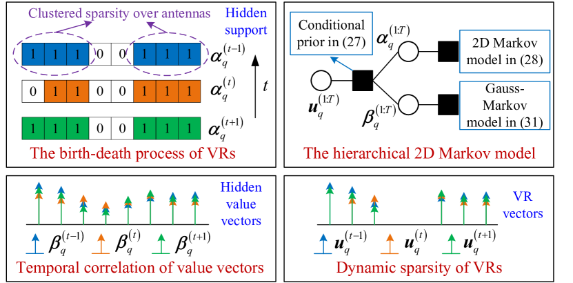
Figure 3: Hierarchical 2D Markov model to exploit the dynamic sparsity of VRs.

The specific sparse structure of hidden support vectors is affected by the value of $\left\{p_{01}^{T},p_{10}^{T},p_{01}^{S},p_{10}^{S}\right\}$. Specifically, a smaller $p_{01}^{S}$ leads to a larger average cluster size of visible antennas, a smaller $p_{01}^{S}$ implies a larger average gap between two adjacent visible clusters, and smaller $p_{01}^{T}$ and $p_{10}^{T}$ indicate a stronger temporal correlation of VRs. Therefore, the 2-D Markov model is very suitable to describe the dynamic sparsity of VRs.

As shown in Fig. 3, the received power of antennas change smoothly over time. And thus, we use a spatially independent steady-state Gauss-Markov process to model the temporal correlation of the hidden value vectors [3],

$$\boldsymbol{\beta}_{q,m}^{\left(t\right)}=\left(1-\varepsilon\right)\left(\boldsymbol{\beta}_{q,m}^{\left(t-1\right)}-\zeta\right)+\varepsilon\varpi_{q,m}^{\left(t\right)}+\zeta,$$ (30)

where $\varepsilon\in\left[0,1\right]$ controls the strength of temporal correlation, $\varpi_{q,m}^{\left(t\right)}\sim\mathcal{N}\left(0,\sigma^{2}\right)$ is the Gaussian perturbation with variance $\sigma^{2}$, and $\zeta\in\mathbb{R}+$ is the mean of the random process. Then, $p\left(\boldsymbol{\beta}_{q}^{\left(1:T\right)}\right),\forall q$ is given by

$$p\left(\boldsymbol{\beta}_{q}^{\left(1:T\right)}\right)=\prod_{m=1}^{M}\left(p\left(\boldsymbol{\beta}_{q,m}^{\left(1\right)}\right)\prod_{t=2}^{T}p\left(\boldsymbol{\beta}_{q,m}^{\left(t\right)}\mid\boldsymbol{\beta}_{q,m}^{\left(t-1\right)}\right)\right),$$ (31)

where the initial distribution is $\boldsymbol{\beta}_{q,m}^{\left(1\right)}\sim\mathcal{N}\left(\boldsymbol{\beta}_{q,m}^{\left(1\right)};\zeta,\frac{\varepsilon\sigma^{2}}{2-\varepsilon}\right)$, and the conditional distribution is given by

$$p\left(\boldsymbol{\beta}_{q,m}^{\left(t\right)}\mid\boldsymbol{\beta}_{q,m}^{\left(t-1\right)}\right)=\mathcal{N}\left(\boldsymbol{\beta}_{q,m}^{\left(t\right)};\left(1-\varepsilon\right)\boldsymbol{\beta}_{q,m}^{\left(t-1\right)}+\varepsilon\zeta,\varepsilon^{2}\sigma^{2}\right).$$

Although the prior distribution in (31) cannot ensure $u_{q,m}^{\left(t\right)}$ is non-negative, the MAP estimate of $u_{q,m}^{\left(t\right)}$ must satisfy $\hat{u}_{q,m}^{\left(t\right)}\geq 0$, since it is obtained based on both the estimated posterior distribution and the constraint $u_{q,m}^{\left(t\right)}\geq 0$, as presented in (49).

III-C Channel Tracking Problem Formulation

Based on the polar-delay domain sparse representation in (18), the received signal in (14) can be reformulated into the following bilinear measurement process:

$$\tilde{\boldsymbol{y}}^{\left(t\right)}=\mathbf{F}\left(\mathbf{\Xi}^{\left(t\right)},\mathbf{U}^{\left(t\right)}\right)\boldsymbol{x}^{\left(t\right)}+\tilde{\boldsymbol{z}}^{\left(t\right)},t=1,\ldots,T,$$ (32)

where the observation $\tilde{\boldsymbol{y}}^{\left(t\right)}$ is linear w.r.t. $\boldsymbol{x}^{\left(t\right)}$ and $\mathbf{U}^{\left(t\right)}$. At each time $t$, the goal is to obtain the MAP estimate of the channel vector $\boldsymbol{x}^{\left(t\right)}$, the VR $\mathbf{U}^{\left(t\right)}$, and the grid parameters $\mathbf{\Xi}^{\left(t\right)}$ based on all the previous observations up to time $t$, i.e.,

$$\boldsymbol{x}_{\textrm{MAP}}^{\left(t\right)},\mathbf{U}_{\textrm{MAP}}^{\left(t\right)},\mathbf{\Xi}_{\textrm{MAP}}^{\left(t\right)}=\underset{\mathbf{\Theta}^{\left(t\right)},\mathbf{\Xi}^{\left(t\right)}}{\arg\max}\ln p\left(\tilde{\boldsymbol{y}}^{\left(1:t\right)},\mathbf{\Theta}^{\left(t\right)};\mathbf{\Xi}^{\left(t\right)}\right),$$ (33)

where $\mathbf{\Theta}^{\left(t\right)}\triangleq\left\{\boldsymbol{x}^{\left(t\right)},\boldsymbol{\rho}^{\left(t\right)},\boldsymbol{s}^{\left(t\right)},\gamma^{\left(t\right)},\mathbf{U}^{\left(t\right)},\boldsymbol{\alpha}_{1:Q}^{\left(t\right)},\boldsymbol{\beta}_{1:Q}^{\left(t\right)}\right\}$ is the collection of random variables at time $t$.

One possible solution is to store all the available observations $\tilde{\boldsymbol{y}}^{\left(1:t\right)}$ and perform a joint estimation of $\boldsymbol{x}^{\left(t\right)}$, $\mathbf{U}^{\left(t\right)}$, and $\mathbf{\Xi}^{\left(t\right)}$ at each time $t$. However, the memory cost and computational complexity of such a brute-force solution would become unacceptable for a large $t$. To address this challenge, we decompose and approximate the joint distribution $p\left(\tilde{\boldsymbol{y}}^{\left(1:t\right)},\mathbf{\Theta}^{\left(t\right)};\mathbf{\Xi}^{\left(t\right)}\right)$ to make it only involve the probability density function (PDF) of the current random variables $\mathbf{\Theta}^{\left(t\right)}$, the current observation $\tilde{\boldsymbol{y}}^{\left(t\right)}$, and the messages passed from time $t-1$, based on which a more efficient algorithm can be designed. In particular, we have

$$p\left(\tilde{\boldsymbol{y}}^{\left(1:t\right)},\mathbf{\Theta}^{\left(t\right)};\mathbf{\Xi}^{\left(t\right)}\right)$$

$$\propto \check{p}^{\left(t\right)}\sum_{\boldsymbol{s}^{(t-1)}}\sum_{\boldsymbol{\alpha}_{1:Q}^{\left(t-1\right)}}\int_{\boldsymbol{\beta}_{1:Q}^{\left(t-1\right)}}p\left(\boldsymbol{s}^{\left(t-1\right)},\boldsymbol{\alpha}_{1:Q}^{\left(t-1\right)},\boldsymbol{\beta}_{1:Q}^{\left(t-1\right)}\mid\tilde{\boldsymbol{y}}^{\left(1:t-1\right)}\right)$$

$$\times p\left(\boldsymbol{s}^{\left(t\right)}\mid\boldsymbol{s}^{\left(t-1\right)}\right)\prod_{q=1}^{Q}p\left(\boldsymbol{\alpha}_{q}^{\left(t\right)}|\boldsymbol{\alpha}_{q}^{\left(t-1\right)}\right)p\left(\boldsymbol{\beta}_{q}^{\left(t\right)}|\boldsymbol{\beta}_{q}^{\left(t-1\right)}\right)$$

$$\approx \check{p}^{\left(t\right)}\underbrace{\sum_{\boldsymbol{s}^{(t-1)}}q\left(\boldsymbol{s}^{\left(t-1\right)}\right)p\left(\boldsymbol{s}^{\left(t\right)}|\boldsymbol{s}^{\left(t-1\right)}\right)}_{\hat{p}\left(\boldsymbol{s}^{\left(t\right)}\right)}$$

$$\times\prod_{q=1}^{Q}\underbrace{\sum_{\boldsymbol{\alpha}_{q}^{\left(t-1\right)}}q\left(\boldsymbol{\alpha}_{q}^{\left(t-1\right)}\right)p\left(\boldsymbol{\alpha}_{q}^{\left(t\right)}|\boldsymbol{\alpha}_{q}^{\left(t-1\right)}\right)}_{\hat{p}\left(\boldsymbol{\alpha}_{q}^{\left(t\right)}\right)}$$

$$\times\prod_{q=1}^{Q}\underbrace{\int_{\boldsymbol{\beta}_{q}^{\left(t-1\right)}}q\left(\boldsymbol{\beta}_{q}^{\left(t-1\right)}\right)p\left(\boldsymbol{\beta}_{q}^{\left(t\right)}|\boldsymbol{\beta}_{q}^{\left(t-1\right)}\right)}_{\hat{p}\left(\boldsymbol{\beta}_{q}^{\left(t\right)}\right)}$$

$$\triangleq \check{p}\left(\tilde{\boldsymbol{y}}^{\left(t\right)},\mathbf{\Theta}^{\left(t\right)};\mathbf{\Xi}^{\left(t\right)}\right),$$ (34)

where $\check{p}^{\left(t\right)}$ is given by

$$\check{p}^{\left(t\right)}\triangleq p\left(\tilde{\boldsymbol{y}}^{\left(t\right)}\mid\boldsymbol{x}^{\left(t\right)},\mathbf{U}^{\left(t\right)},\gamma^{\left(t\right)};\mathbf{\Xi}^{\left(t\right)}\right)p\left(\gamma^{\left(t\right)}\right)$$

$$\times p\left(\boldsymbol{x}^{\left(t\right)}|\boldsymbol{\rho}^{\left(t\right)}\right)p\left(\boldsymbol{\rho}^{\left(t\right)}|\boldsymbol{s}^{\left(t\right)}\right)\prod_{q=1}^{Q}p\left(\boldsymbol{u}_{q}^{\left(t\right)}\mid\boldsymbol{\alpha}_{q}^{\left(t\right)},\boldsymbol{\beta}_{q}^{\left(t\right)}\right),$$ (35)

with the likelihood function in (35) given by $\mathcal{CN}\left(\tilde{\boldsymbol{y}}^{\left(t\right)};\mathbf{F}\left(\mathbf{\Xi}^{\left(t\right)},\mathbf{U}^{\left(t\right)}\right)\boldsymbol{x}^{\left(t\right)},1/\gamma^{\left(t\right)}\mathbf{I}_{MN}\right)$. Note that we cannot obtain the exact posterior distribution $p\left(\boldsymbol{s}^{\left(t-1\right)},\boldsymbol{\alpha}_{1:Q}^{\left(t-1\right)},\boldsymbol{\beta}_{1:Q}^{\left(t-1\right)}\mid\tilde{\boldsymbol{y}}^{\left(1:t-1\right)}\right)$ in (34) since the factor graph corresponding to the joint distribution $p\left(\tilde{\boldsymbol{y}}^{\left(1:t-1\right)},\mathbf{\Theta}^{\left(1:t-1\right)};\mathbf{\Xi}^{\left(1:t-1\right)}\right)$ contains loops. Therefore, we turn to calculate the approximate posterior of $\boldsymbol{s}^{\left(t-1\right)}$, $\boldsymbol{\alpha}_{q}^{\left(t-1\right)}$, and $\boldsymbol{\beta}_{q}^{\left(t-1\right)}$, denoted by $q\left(\boldsymbol{s}^{\left(t-1\right)}\right)$, $q\left(\boldsymbol{\alpha}_{q}^{\left(t-1\right)}\right)$, and $q\left(\boldsymbol{\beta}_{q}^{\left(t-1\right)}\right)$, respectively. Then $\hat{p}\left(\boldsymbol{s}^{\left(t\right)}\right)$, $\hat{p}\left(\boldsymbol{\alpha}_{q}^{\left(t\right)}\right)$, and $\hat{p}\left(\boldsymbol{\beta}_{q}^{\left(t\right)}\right)$ can be viewed as the effective prior information for $\boldsymbol{s}^{\left(t\right)}$, $\boldsymbol{\alpha}_{q}^{\left(t\right)}$, and $\boldsymbol{\beta}_{q}^{\left(t\right)}$ obtained by prediction from time $t-1$, which summarize all information contributed by $\tilde{\boldsymbol{y}}^{\left(1:t-1\right)}$. Using (34), the MAP problem in (33) can be simplified into

$$\boldsymbol{x}_{\textrm{MAP}}^{\left(t\right)},\mathbf{U}_{\textrm{MAP}}^{\left(t\right)},\mathbf{\Xi}_{\textrm{MAP}}^{\left(t\right)}= \underset{\mathbf{\Theta}^{\left(t\right)},\mathbf{\Xi}^{\left(t\right)}}{\arg\max}\ln\check{p}\left(\tilde{\boldsymbol{y}}^{\left(t\right)},\mathbf{\Theta}^{\left(t\right)};\mathbf{\Xi}^{\left(t\right)}\right).$$ (36)

However, it is still intractable to directly solve the MAP estimation problem in (36) since different variables and their latent variables have quite different priors and they are complicatedly coupled with the likelihood function. In the next section, we shall propose the DA-MAP framework to overcome this challenge.

IV Dynamic Alternating MAP Framework

IV-A Outline of DA-MAP Framework

The dynamic alternating MAP framework adopts the idea of alternating optimization to solve the MAP problem in (36). As illustrated in Fig. 4, the DA-MAP consists of four basic modules: channel estimation module, VR detection module, grid update module, and temporal correlated module. In the following, we give a brief introduction of each basic module.

• Channel estimation module: The low-complexity IF-VBI estimator is used to achieve channel estimation. Specifically, given $\hat{p}\left(\boldsymbol{s}^{\left(t\right)}\right)$ from time $t-1$, $\hat{\mathbf{U}}^{\left(t\right)}$ from VR detection module, and $\hat{\mathbf{\Xi}}^{\left(t\right)}$ from grid update module, the IF-VBI performs Bayesian inference to compute the posterior distribution of $\boldsymbol{x}^{\left(t\right)}$, $\boldsymbol{\rho}^{\left(t\right)}$, $\boldsymbol{s}^{\left(t\right)}$, and $\gamma^{\left(t\right)}$ in an alternative way.

• VR detection module: It is the Turbo-CS algorithm that combines the linear minimum-mean-square-error (LMMSE) module and the structured sparse inference module via the turbo approach. Given $\hat{p}\left(\boldsymbol{\alpha}_{q}^{\left(t\right)}\right)$ and $\hat{p}\left(\boldsymbol{\beta}_{q}^{\left(t\right)}\right)$ from time $t-1$, $\hat{\boldsymbol{x}}^{\left(t\right)}$and $\hat{\gamma}^{\left(t\right)}$ from channel estimation module, and $\hat{\mathbf{\Xi}}^{\left(t\right)}$ from grid update module, the VR detection module calculates the marginal posterior distribution of $\boldsymbol{u}_{q}^{\left(t\right)}$, $\boldsymbol{\alpha}_{q}^{\left(t\right)}$, and $\boldsymbol{\beta}_{q}^{\left(t\right)}$, $\forall q$.

• Grid update module: It uses the gradient ascent method to refine the polar-delay domain grid. Given $\hat{\mathbf{\Xi}}^{\left(t-1\right)}$ from time $t-1$, $\hat{\boldsymbol{x}}^{\left(t\right)}$and $\hat{\gamma}^{\left(t\right)}$ from channel estimation module, and $\hat{\mathbf{U}}^{\left(t\right)}$ from VR detection module, calculate the gradient of $\ln p\left(\tilde{\boldsymbol{y}}^{\left(t\right)}\mid\hat{\boldsymbol{x}}^{\left(t\right)},\hat{\mathbf{U}}^{\left(t\right)},\hat{\gamma}^{\left(t\right)};\mathbf{\Xi}^{\left(t\right)}\right)$, and then update grid parameters via gradient ascent.

• Temporal correlated module: Given $q\left(\boldsymbol{s}^{\left(t\right)}\right)$ from channel estimation module, $q\left(\boldsymbol{\alpha}_{q}^{\left(t\right)}\right)$ and $q\left(\boldsymbol{\beta}_{q}^{\left(t\right)}\right)$ from VR detection module, it calculates $\hat{p}\left(\boldsymbol{s}^{\left(t+1\right)}\right)$, $\hat{p}\left(\boldsymbol{\alpha}_{q}^{\left(t+1\right)}\right)$, and $\hat{p}\left(\boldsymbol{\beta}_{q}^{\left(t+1\right)}\right)$ as the prior for time $t+1$.

At each time $t$, the channel estimation module, VR detection module, and grid update module work alternatively until convergence to a stationary point of (36). Then, the temporal correlated module calculates the prior information for time $t+1$. The proposed DA-MAP can be viewed as an extension of the alternating MAP framework in [17] by: 1) extending from 0/1 VR detection to continuous VR detection with power change; 2) extending from the single-frame channel estimation to multi-frame channel tracking.

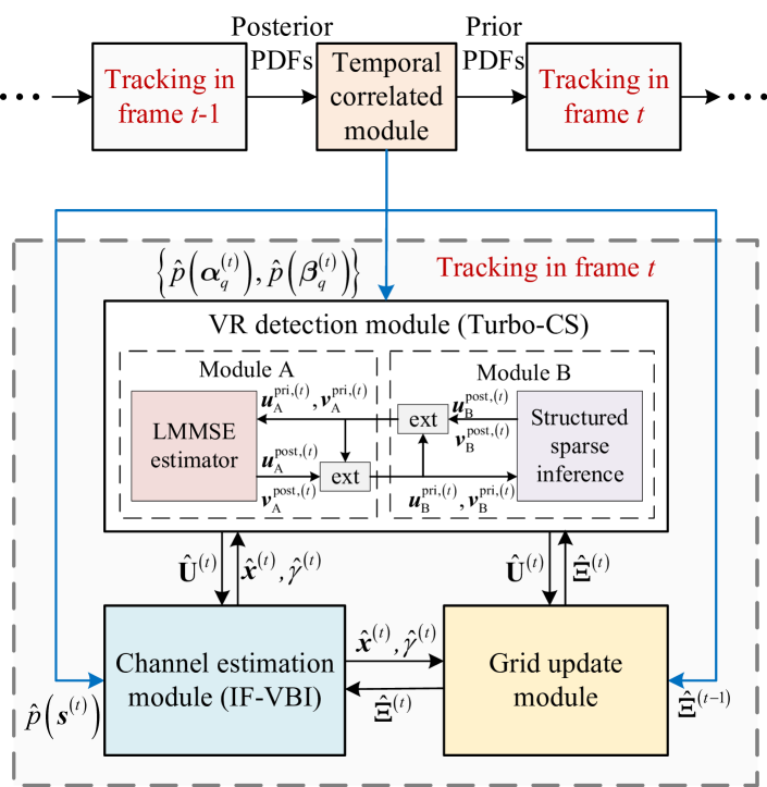
Figure 4: The DA-MAP algorithmic framework with its four basic modules.

IV-B Channel Estimation Module (IF-VBI)

Given $\hat{\mathbf{U}}^{\left(t\right)}$ and $\hat{\mathbf{\Xi}}^{\left(t\right)}$, the transform matrix $\mathbf{F}\left(\hat{\mathbf{\Xi}}^{\left(t\right)},\hat{\mathbf{U}}^{\left(t\right)}\right)$ in (32) is fixed. Now the observation in (32) can be simplified into $\tilde{\boldsymbol{y}}^{\left(t\right)}=\mathbf{F}\boldsymbol{x}^{\left(t\right)}+\tilde{\boldsymbol{z}}^{\left(t\right)}$, where $\hat{\mathbf{\Xi}}^{\left(t\right)}$ and $\hat{\mathbf{U}}^{\left(t\right)}$ are omitted in $\mathbf{F}\left(\hat{\mathbf{\Xi}}^{\left(t\right)},\hat{\mathbf{U}}^{\left(t\right)}\right)$ for simplicity. The sub-problem of channel estimation is a standard compressive sensing problem that can be solved by many existing CS-based methods. We adopt the IF-VBI algorithm to achieve a good trade-off between the estimation performance and computational complexity.

The IF-VBI avoids the complicated matrix inverse each iteration via minimizing a relaxed Kullback-Leibler divergence. The prior distribution $\hat{p}\left(\boldsymbol{s}^{\left(t\right)}\right)$ from time $t-1$ can speed up convergence of the IF-VBI algorithm. Due the the space limitation, please refer to our previous work in [17, 19] for more details of the IF-VBI.

IV-C VR Detection Module (Turbo-CS)

Given $\hat{\boldsymbol{x}}^{\left(t\right)}$, $\hat{\gamma}^{\left(t\right)}$, and $\hat{\mathbf{\Xi}}^{\left(t\right)}$, the observation in (32) can be rewritten into

$$\tilde{\boldsymbol{y}}^{\left(t\right)}=\left[\mathbf{B}\odot\left(\mathbf{U}^{\left(t\right)}\otimes\boldsymbol{1}_{N\times 1}\right)\right]\hat{\boldsymbol{x}}^{\left(t\right)}+\tilde{\boldsymbol{z}}^{\left(t\right)},$$ (37)

where $\hat{\mathbf{\Xi}}^{\left(t\right)}$ is omitted in $\mathbf{B}\left(\hat{\mathbf{\Xi}}^{\left(t\right)}\right)$ to simply the notation. Define $\boldsymbol{\Phi}_{m}\triangleq\left\{\left(m-1\right)N+n\mid n=1,\ldots,N\right\}$, the received signal of the $m\textrm{-th}$ antenna is given by

$$\tilde{\boldsymbol{y}}_{m}^{\left(t\right)} =\underbrace{\left[\mathbf{B}_{m}\odot\left(\boldsymbol{1}_{N\times 1}\left(\hat{\boldsymbol{x}}^{\left(t\right)}\right)^{T}\right)\right]}_{\mathbf{G}_{m}^{\left(t\right)}}\left(\mathbf{U}_{m,:}^{\left(t\right)}\right)^{T}+\tilde{\boldsymbol{z}}_{m}^{\left(t\right)},$$ (38)

where $\tilde{\boldsymbol{y}}_{m}^{\left(t\right)}\in\mathbb{C}^{N\times 1}$ and $\tilde{\boldsymbol{z}}_{m}^{\left(t\right)}\in\mathbb{C}^{N\times 1}$ denote the $m\textrm{-th}$ column of $\tilde{\mathbf{Y}}^{\left(t\right)}$ and $\tilde{\mathbf{Z}}^{\left(t\right)}$ in (13), respectively, $\mathbf{B}_{m}\triangleq\left[\mathbf{B}_{k,:}\right]_{k\in\boldsymbol{\Phi}_{m}}$ with $\mathbf{B}_{k,:}$ denote the $k\textrm{-th}$ row of $\mathbf{B}$, and $\mathbf{U}_{m,:}^{\left(t\right)}\triangleq\left[u_{1,m}^{\left(t\right)},\ldots,u_{Q,m}^{\left(t\right)}\right]$ represents the $m\textrm{-th}$ row of $\mathbf{U}^{\left(t\right)}$.

Note that $\hat{\boldsymbol{x}}^{\left(t\right)}$ has a few non-zero elements since the number of channel paths is much smaller than the number of grid points, i.e., $L^{\left(t\right)}\ll Q$. Therefore, the sensing matrix $\mathbf{G}_{m}^{\left(t\right)}$ also has many close-to-zero columns and is ill-conditioned, which makes it difficult to estimate $\mathbf{U}_{m,:}^{\left(t\right)}$ accurately. To address this issue, we introduce a polar-delay domain filtering method. Specifically, we compare the energy of each element of $\hat{\boldsymbol{x}}^{\left(t\right)}$ with an energy threshold $\eta>0$. Define $\mathbf{\Omega}^{\left(t\right)}\triangleq\left\{q\mid\forall\left\|\hat{x}_{q}^{\left(t\right)}\right\|^{2}>\eta\right\}$ as the index set of the elements with the energy larger than the threshold. Then, we only retain the columns indexed by $\mathbf{\Omega}^{\left(t\right)}$ in $\mathbf{G}_{m}^{\left(t\right)}$ and delete other columns that are close to zero. The sensing matrix after clipping, denoted by $\tilde{\mathbf{G}}_{m}^{\left(t\right)}\in\mathbb{C}^{N\times\left|\mathbf{\Omega}^{\left(t\right)}\right|}$, is well-conditioned now. Moreover, we only need to estimate $\ddot{\boldsymbol{u}}_{m}^{\left(t\right)}\triangleq\left[u_{q,m}^{\left(t\right)}\right]_{q\in\mathbf{\Omega}^{\left(t\right)}}$ instead of $\mathbf{U}_{m,:}^{\left(t\right)}$. This is because the energy of $\hat{x}_{q}^{\left(t\right)}$ is close to zero for $q\notin\mathbf{\Omega}^{\left(t\right)}$, which implies that there is no scatterer lying around the $q\textrm{-th}$ polar-delay domain grid. In this case, we have $u_{q,m}^{\left(t\right)}=0,\forall m$.

Based on the polar-delay domain filtering, the signal model in (38) is rewritten as

$$\tilde{\boldsymbol{y}}_{m}^{\left(t\right)}=\tilde{\mathbf{G}}_{m}^{\left(t\right)}\ddot{\boldsymbol{u}}_{m}^{\left(t\right)}+\tilde{\boldsymbol{z}}_{m}^{\left(t\right)},\forall m,$$ (39)

which is a complex-valued observation model while $\ddot{\boldsymbol{u}}_{m}$ is real-valued. And thus, we transform (39) into a real-valued one,

$$\boldsymbol{\ddot{y}}_{m}^{\left(t\right)}=\mathbf{\ddot{G}}_{m}^{\left(t\right)}\boldsymbol{\ddot{u}}_{m}^{\left(t\right)}+\boldsymbol{\ddot{z}}_{m}^{\left(t\right)},\forall m,$$ (40)

where $\boldsymbol{\ddot{y}}_{m}^{\left(t\right)}\triangleq\left[\Re\left(\boldsymbol{\ddot{y}}_{m}^{\left(t\right)}\right)^{T},\Im\left(\boldsymbol{\ddot{y}}_{m}^{\left(t\right)}\right)^{T}\right]^{T},$ and $\mathbf{\ddot{G}}_{m}^{\left(t\right)}$ and $\boldsymbol{\ddot{z}}_{m}^{\left(t\right)}$ are defined similarly. The sub-problem of VR detection is to obtain the posterior distribution of $\ddot{\boldsymbol{u}}_{m},\forall m$ based on the linear observations in (40) and structured sparse priors. Inspired by the turbo framework [20], we develop a Turbo-CS algorithm to achieve VR detection in a parallel fashion.

As shown in Fig. 4, the Turbo-CS has two basic modules: Module A and Module B. Specifically, Module A performs the LMMSE estimation based on the observation of each antenna and messages from Module B, while Module B performs structured sparse inference using the hierarchical 2D Markov prior information and messages from Module A. The two modules exchange messages with each other until convergence.

IV-C1 LMMSE in Module A

The prior distribution of $\boldsymbol{\ddot{u}}_{m}^{\left(t\right)}$ in Module A is $\mathcal{N}\left(\boldsymbol{\ddot{u}}_{m}^{\left(t\right)};\boldsymbol{u}_{\textrm{A},m}^{\textrm{pri},\left(t\right)},\boldsymbol{v}_{\textrm{A},m}^{\textrm{pri,$\left(t\right)$}}\right)$, where $\boldsymbol{u}_{\textrm{A},m}^{\textrm{pri},\left(t\right)}$ and $\boldsymbol{v}_{\textrm{A},m}^{\textrm{pri,$\left(t\right)$}}$ are extrinsic messages passed from Module B. According to the LMMSE estimation, the posterior distribution of $\boldsymbol{\ddot{u}}_{m}^{\left(t\right)}$ is a Gaussian distribution with the posterior mean and covariance given by

$$\mathbf{V}_{\textrm{A},m}^{\textrm{post},\left(t\right)} =\left(\hat{\gamma}^{\left(t\right)}\left(\mathbf{\ddot{G}}_{m}^{\left(t\right)}\right)^{T}\mathbf{\ddot{G}}_{m}^{\left(t\right)}+\textrm{diag}\left(1/\boldsymbol{v}_{\textrm{A},m}^{\textrm{pri,$\left(t\right)$}}\right)\right)^{-1},$$

$$\boldsymbol{u}_{\textrm{A},m}^{\textrm{post},\left(t\right)} =\mathbf{V}_{\textrm{A},m}^{\textrm{post},\left(t\right)}\left(\frac{\boldsymbol{u}_{\textrm{A},m}^{\textrm{pri},\left(t\right)}}{\boldsymbol{v}_{\textrm{A},m}^{\textrm{pri,$\left(t\right)$}}}+\hat{\gamma}^{\left(t\right)}\left(\mathbf{\ddot{G}}_{m}^{\left(t\right)}\right)^{T}\boldsymbol{\ddot{y}}_{m}^{\left(t\right)}\right).$$ (41)

Then, Module A outputs extrinsic messages to Module B as

$$\boldsymbol{u}_{\textrm{B},m}^{\textrm{pri},\left(t\right)} =\boldsymbol{v}_{\textrm{B},m}^{\textrm{pri,$\left(t\right)$}}\left(\boldsymbol{u}_{\textrm{A},m}^{\textrm{post},\left(t\right)}/\boldsymbol{v}_{\textrm{A},m}^{\textrm{post},\left(t\right)}-\boldsymbol{u}_{\textrm{A},m}^{\textrm{pri},\left(t\right)}/\boldsymbol{v}_{\textrm{A},m}^{\textrm{pri,$\left(t\right)$}}\right),$$

$$\boldsymbol{v}_{\textrm{B},m}^{\textrm{pri,$\left(t\right)$}} =1/\left(1/\boldsymbol{v}_{\textrm{A},m}^{\textrm{post},\left(t\right)}-1/\boldsymbol{v}_{\textrm{A},m}^{\textrm{pri,$\left(t\right)$}}\right),$$ (42)

where $\boldsymbol{v}_{\textrm{A},m}^{\textrm{post},\left(t\right)}=\textrm{diag}\left(\mathbf{V}_{\textrm{A},m}^{\textrm{post},\left(t\right)}\right)$. The computational complexity of Module A is dominated by the matrix inverse in the calculation of $\mathbf{V}_{\textrm{A},m}^{\textrm{post},\left(t\right)}$. Fortunately, the dimension of $\mathbf{V}_{\textrm{A},m}^{\textrm{post},\left(t\right)}$ is very small thanks to the polar-delay domain filtering ($\left|\mathbf{\Omega}^{\left(t\right)}\right|$ is comparable to the number of channel paths). Besides, $M$ LMMSE estimators can work in a parallel fashion. Therefore, Module A is highly efficient with a relatively low computational overhead.

IV-C2 Structured Sparse Inference in Module B

In Module B, the extrinsic message $\boldsymbol{u}_{\textrm{B},m}^{\textrm{pri},\left(t\right)}$ is viewed as an AWGN observation of $\boldsymbol{\ddot{u}}_{m}^{\left(t\right)}$ [20]:

$$u_{\textrm{B},q,m}^{\textrm{pri},\left(t\right)}=u_{q,m}^{\left(t\right)}+n_{q,m}^{\left(t\right)},q\in\mathbf{\Omega}^{\left(t\right)},$$ (43)

where $n_{q,m}^{\left(t\right)}\sim\mathcal{N}\left(n_{q,m}^{\left(t\right)};0,v_{\textrm{B},q,m}^{\textrm{pri,$\left(t\right)$}}\right)$ is the equivalent noise, $u_{\textrm{B},q,m}^{\textrm{pri},\left(t\right)}$ and $v_{\textrm{B},q,m}^{\textrm{pri},\left(t\right)}$ represent the element of $\boldsymbol{u}_{\textrm{B},m}^{\textrm{pri},\left(t\right)}$ and $\boldsymbol{v}_{\textrm{B},m}^{\textrm{pri},\left(t\right)}$, respectively. Then, the joint distribution associated with Module B is given by

$$p_{\textrm{B}}= \prod_{q\in\mathbf{\Omega}^{\left(t\right)}}^{Q}p\left(\boldsymbol{u}_{q}^{\left(t\right)}\mid\boldsymbol{\alpha}_{q}^{\left(t\right)},\boldsymbol{\beta}_{q}^{\left(t\right)}\right)\hat{p}\left(\boldsymbol{\alpha}_{q}^{\left(t\right)}\right)\hat{p}\left(\boldsymbol{\beta}_{q}^{\left(t\right)}\right)$$

$$\times\prod_{m=1}^{M}p\left(u_{\textrm{B},q,m}^{\textrm{pri},\left(t\right)}\mid u_{q,m}^{\left(t\right)}\right).$$ (44)

The factor graph of the joint distribution is shown in Fig. 5, where the associated factor nodes are listed in Table I. According to the structure of the joint distribution in (44), the whole factor graph consists of $\left|\mathbf{\Omega}^{\left(t\right)}\right|$ independent sub-graphs with the same internal structure, denoted by $\mathcal{G}_{q}^{\left(t\right)}$ for $q\in\mathbf{\Omega}^{\left(t\right)}$. We use the sum-product rule [34] to perform message passing over each sub-graph $\mathcal{G}_{q}^{\left(t\right)}$.

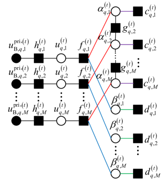
Figure 5: The structure of the sub-graph $\mathcal{G}_{q}^{\left(t\right)},q\in\mathbf{\Omega}^{\left(t\right)}$.

TABLE I: Factors, distributions, and functional forms in Fig. 5.

Factor	Distribution	Functional form
$h_{q,m}^{\left(t\right)}$	$p\left(u_{\textrm{B},q,m}^{\textrm{pri},\left(t\right)}\mid u_{q,m}^{\left(t\right)}\right)$	$\mathcal{N}\left(u_{\textrm{B},q,m}^{\textrm{pri},\left(t\right)};u_{q,m}^{\left(t\right)},v_{\textrm{B},q,m}^{\textrm{pri,$\left(t\right)$}}\right)$
$f_{q,m}^{\left(t\right)}$	$p\left(u_{q,m}^{\left(t\right)}\mid\alpha_{q,m}^{\left(t\right)},\beta_{q,m}^{\left(t\right)}\right)$	$\delta\left(u_{q,m}^{\left(t\right)}-\alpha_{q,m}^{\left(t\right)}\beta_{q,m}^{\left(t\right)}\right)$
$c_{q,m}^{\left(t\right)}$	$\hat{p}\left(\alpha_{q,m}^{\left(t\right)}\right)$	given in (53)
$g_{q,m}^{\left(t\right)}$	$p\left(\alpha_{q,m}^{\left(t\right)}\mid\alpha_{q,m-1}^{\left(t\right)}\right)$	given in (29c) and (29d)
$d_{q,m}^{\left(t\right)}$	$\hat{p}\left(\beta_{q,m}^{\left(t\right)}\right)$	given in (55)

Specifically, we first calculate messages over $u_{q,m}^{\left(t\right)}/\beta_{q,m}^{\left(t\right)}\rightarrow f_{q,m}^{\left(t\right)}\rightarrow\alpha_{q,m}^{\left(t\right)}$. Then, forward-backward message passing is performed over the Markov chain $\alpha_{q,1}^{\left(t\right)}\rightarrow\alpha_{q,2}^{\left(t\right)}\rightarrow\ldots\rightarrow\alpha_{q,M}^{\left(t\right)}$. Finally, we perform message passing over $\alpha_{q,m}^{\left(t\right)}\rightarrow f_{q,m}^{\left(t\right)}\rightarrow u_{q,m}^{\left(t\right)}/\beta_{q,m}^{\left(t\right)}$. The marginal posterior distribution of $u_{q,m}^{\left(t\right)}$, $\alpha_{q,m}^{\left(t\right)}$ and $\beta_{q,m}^{\left(t\right)}$ can be computed by

$$q\left(u_{q,m}^{\left(t\right)}\right) \propto\upsilon_{f_{q,m}^{\left(t\right)}\rightarrow u_{q,m}^{\left(t\right)}}\left(u_{q,m}^{\left(t\right)}\right)\upsilon_{u_{q,m}^{\left(t\right)}\rightarrow f_{q,m}^{\left(t\right)}}\left(u_{q,m}^{\left(t\right)}\right),$$ (45)

$$q\left(\alpha_{q,m}^{\left(t\right)}\right) \propto\upsilon_{f_{q,m}^{\left(t\right)}\rightarrow\alpha_{q,m}^{\left(t\right)}}\left(\alpha_{q,m}^{\left(t\right)}\right)\upsilon_{\alpha_{q,m}^{\left(t\right)}\rightarrow f_{q,m}^{\left(t\right)}}\left(\alpha_{q,m}^{\left(t\right)}\right),$$ (46)

$$q\left(\beta_{q,m}^{\left(t\right)}\right) \propto\upsilon_{f_{q,m}^{\left(t\right)}\rightarrow\beta_{q,m}^{\left(t\right)}}\left(\beta_{q,m}^{\left(t\right)}\right)\upsilon_{\beta_{q,m}^{\left(t\right)}\rightarrow f_{q,m}^{\left(t\right)}}\left(\beta_{q,m}^{\left(t\right)}\right),$$ (47)

where $\upsilon_{f_{q,m}^{\left(t\right)}\rightarrow u_{q,m}^{\left(t\right)}}$ means the message passed from factor node $f_{q,m}^{\left(t\right)}$ to variable node $u_{q,m}^{\left(t\right)}$. And the posterior mean $u_{\textrm{B},q,m}^{\textrm{post},\left(t\right)}$ and variance $v_{\textrm{B},q,m}^{\textrm{post},\left(t\right)}$ of $u_{q,m}^{\left(t\right)}$ can be obtained based on (45). Denote $\boldsymbol{u}_{\textrm{B},m}^{\textrm{post},\left(t\right)}\triangleq\left[u_{\textrm{B},q,m}^{\textrm{post},\left(t\right)}\right]_{q\in\mathbf{\Omega}^{\left(t\right)}}$ and $\boldsymbol{v}_{\textrm{B},m}^{\textrm{post},\left(t\right)}\triangleq\left[v_{\textrm{B},q,m}^{\textrm{post},\left(t\right)}\right]_{q\in\mathbf{\Omega}^{\left(t\right)}}$, the extrinsic message passed from Module A to Module B is given by

$$\boldsymbol{u}_{\textrm{A},m}^{\textrm{pri},\left(t\right)} =\boldsymbol{v}_{\textrm{A},m}^{\textrm{pri,$\left(t\right)$}}\left(\boldsymbol{u}_{\textrm{B},m}^{\textrm{post},\left(t\right)}/\boldsymbol{v}_{\textrm{B},m}^{\textrm{post},\left(t\right)}-\boldsymbol{u}_{\textrm{B},m}^{\textrm{pri},\left(t\right)}/\boldsymbol{v}_{\textrm{B},m}^{\textrm{pri,$\left(t\right)$}}\right),$$

$$\boldsymbol{v}_{\textrm{A},m}^{\textrm{pri,$\left(t\right)$}} =1/\left(1/\boldsymbol{v}_{\textrm{B},m}^{\textrm{post},\left(t\right)}-1/\boldsymbol{v}_{\textrm{B},m}^{\textrm{pri,$\left(t\right)$}}\right).$$ (48)

After convergence of the algorithm, the MAP estimate of $u_{q,m}^{\left(t\right)}\in\left[0,+\infty\right),q\in\mathbf{\Omega}^{\left(t\right)},\forall m$ is updated as

$$\hat{u}_{q,m}^{\left(t\right)}=\begin{cases}u_{\textrm{A},q,m}^{\textrm{post},\left(t\right)},&u_{\textrm{A},q,m}^{\textrm{post},\left(t\right)}\geq 0\\ 0,&u_{\textrm{A},q,m}^{\textrm{post},\left(t\right)}<0\end{cases}.$$ (49)

IV-D Grid Update Module

Given $\hat{\boldsymbol{x}}^{\left(t\right)}$, $\hat{\gamma}^{\left(t\right)}$, and $\hat{\mathbf{U}}^{\left(t\right)}$, the log-likelihood function is given by

$$\mathcal{L}\left(\mathbf{\Xi}^{\left(t\right)}\right) =\ln p\left(\tilde{\boldsymbol{y}}^{\left(t\right)}\mid\hat{\boldsymbol{x}}^{\left(t\right)},\hat{\mathbf{U}}^{\left(t\right)},\hat{\gamma}^{\left(t\right)};\mathbf{\Xi}^{\left(t\right)}\right)$$ (50)

$$=-\hat{\gamma}^{\left(t\right)}\left\|\tilde{\boldsymbol{y}}^{\left(t\right)}-\mathbf{F}\left(\mathbf{\Xi}^{\left(t\right)},\hat{\mathbf{U}}^{\left(t\right)}\right)\hat{\boldsymbol{x}}^{\left(t\right)}\right\|^{2}+C,$$

where $C$ is a constant. It is intractable to directly find the global optimal solution that maximizes $\mathcal{L}\left(\mathbf{\Xi}^{\left(t\right)}\right)$ since it is non-concave w.r.t. $\mathbf{\Xi}^{\left(t\right)}$. And thus, we update grid parameters via gradient ascent. $\mathbf{\Xi}^{\left(t\right)}$ can be divided into $J=3$ blocks with $\mathbf{\Xi}_{1}^{\left(t\right)}=\boldsymbol{\vartheta}^{\left(t\right)}$, $\mathbf{\Xi}_{2}^{\left(t\right)}=\frac{1}{\boldsymbol{r}^{\left(t\right)}}$, and $\mathbf{\Xi}_{3}^{\left(t\right)}=\boldsymbol{\boldsymbol{\tau}}^{\left(t\right)}$ according to different physical meanings. Starting from the initial point $\mathbf{\Xi}_{j}^{\left(t\right)\left(0\right)}=\hat{\mathbf{\Xi}}^{\left(t-1\right)}$, where $\hat{\mathbf{\Xi}}^{\left(t-1\right)}$ is the estimated grid passed from time $t-1$, in the $i\textrm{-th}$ iteration, each block is updated as

$$\mathbf{\Xi}_{j}^{\left(t\right)\left(i\right)}=\mathbf{\Xi}_{j}^{\left(t\right)\left(i-1\right)}+\epsilon_{j}^{\left(i\right)}\left.\tfrac{\partial\mathcal{L}\left(\mathbf{\Xi}_{j}^{\left(t\right)},\mathbf{\Xi}_{-j}^{\left(t\right)\left(i\right)}\right)}{\partial\mathbf{\Xi}_{j}^{\left(t\right)}}\right|{}_{\mathbf{\Xi}_{j}^{\left(t\right)}=\mathbf{\Xi}_{j}^{\left(t\right)\left(i-1\right)}},$$ (51)

where $\mathbf{\Xi}_{-j}^{\left(t\right)\left(i\right)}\triangleq\left(\mathbf{\Xi}_{1}^{\left(t\right)\left(i\right)},\ldots,\mathbf{\Xi}_{j-1}^{\left(t\right)\left(i\right)},\mathbf{\Xi}_{j+1}^{\left(t\right)\left(i-1\right)},\ldots,\mathbf{\Xi}_{J}^{\left(t\right)\left(i-1\right)}\right)$, and $\epsilon_{j}^{\left(i\right)}$ is the step size determined by the Armijo rule.

IV-E Temporal Correlated Module

In this module, we calculate $\hat{p}\left(\boldsymbol{s}^{\left(t+1\right)}\right)$, $\hat{p}\left(\boldsymbol{\alpha}_{q}^{\left(t+1\right)}\right)$, and $\hat{p}\left(\boldsymbol{\beta}_{q}^{\left(t+1\right)}\right)$ as the prior for time $t+1$.

IV-E1 Update of $\hat{p}\left(\boldsymbol{s}^{\left(t+1\right)}\right)$

Given the posterior distribution $q\left(s_{q}^{\left(t\right)}\right),\forall q$ output by the IF-VBI, $\hat{p}\left(s_{q}^{\left(t+1\right)}\right)$ is update as $\hat{p}\left(s_{q}^{\left(t+1\right)}=1\right)=\lambda_{q}^{\left(t+1\right)},$where

$$\lambda_{q}^{\left(t+1\right)}=p_{11}^{x}q\left(s_{q}^{\left(t\right)}=1\right)+p_{01}^{x}q\left(s_{q}^{\left(t\right)}=0\right).$$ (52)

IV-E2 Update of $\hat{p}\left(\boldsymbol{\alpha}_{q}^{\left(t+1\right)}\right)$

Given $q\left(\alpha_{q,m}^{\left(t\right)}\right)$ in (46), $\hat{p}\left(\alpha_{q,m}^{\left(t+1\right)}\right),\forall m$ is calculated as

$$\hat{p}\left(\alpha_{q,m}^{\left(t+1\right)}=1\right)=\begin{cases}\pi_{q,m}^{\textrm{pri},\left(t+1\right)},&q\in\mathbf{\Omega}^{\left(t\right)}\\ \kappa,&q\notin\mathbf{\Omega}^{\left(t\right)}\end{cases},$$ (53)

where

$$\pi_{q,m}^{\textrm{pri},\left(t+1\right)}=p_{11}^{T}q\left(\alpha_{q,m}^{\left(t\right)}=1\right)+p_{01}^{T}q\left(\alpha_{q,m}^{\left(t\right)}=0\right).$$ (54)

IV-E3 Update of $\hat{p}\left(\boldsymbol{\beta}_{q}^{\left(t+1\right)}\right)$

Denote $q\left(\beta_{q,m}^{\left(t\right)}\right)$ in (47) as $\mathcal{N}\left(\beta_{q,m}^{\left(t\right)};\mu_{q,m}^{\textrm{post},\left(t\right)},\nu_{q,m}^{\textrm{post},\left(t\right)}\right)$, we update $\hat{p}\left(\beta_{q,m}^{\left(t+1\right)}\right)$ as

$$\hat{p}\left(\beta_{q,m}^{\left(t+1\right)}\right)=\begin{cases}\mathcal{N}\left(\beta_{q,m}^{\left(t+1\right)};\mu_{q,m}^{\left(t+1\right)},\nu_{q,m}^{\left(t+1\right)}\right),&q\in\mathbf{\Omega}^{\left(t\right)}\\ \mathcal{N}\left(\beta_{q,m}^{\left(t+1\right)};\zeta,\frac{\varepsilon\sigma^{2}}{2-\varepsilon}\right),&q\notin\mathbf{\Omega}^{\left(t\right)}\end{cases},$$ (55)

with $\mu_{q,m}^{\left(t+1\right)}$ and $\nu_{q,m}^{\left(t+1\right)}$ given by

$$\mu_{q,m}^{\left(t+1\right)} =\left(1-\varepsilon\right)\mu_{q,m}^{\textrm{post},\left(t\right)}+\varepsilon\zeta,$$

$$\nu_{q,m}^{\left(t+1\right)} =\left(1-\varepsilon\right)^{2}\nu_{q,m}^{\textrm{post},\left(t\right)}+\varepsilon^{2}\sigma^{2}.$$ (56)

Moreover, the estimated grid $\hat{\mathbf{\Xi}}^{\left(t\right)}$ is used as the initial value of $\mathbf{\Xi}^{\left(t+1\right)}$ to accelerate the convergence speed of signal processing at time $t+1$.

IV-F Complexity Analysis

The DA-MAP algorithm is summarized in Algorithm 1. The IF-VBI estimator avoids the matrix inverse, and its complexity is reduced to $\mathcal{O}\left(MQ\right)$ per iteration [17]. The complexity of the Turbo-CS is dominated by the small-scale matrix inverse in (41), whose complexity is $\mathcal{O}\left(M\left|\mathbf{\Omega}^{\left(t\right)}\right|^{3}\right)$ per iteration. Note that the message passing in Module B of the Turbo-CS and the temporal correlated module is in linear complexity, which is almost negligible. The complexity of the gradient calculation in (51) is $\mathcal{O}\left(Q^{2}\right)$. Let $I_{1}$ and $I_{2}$ represent the inner iteration number of IF-VBI and Turbo-CS, respectively, and let $I$ denote the outer iteration number of DA-MAP. Then, the overall complexity of the DA-MAP is $\mathcal{O}\left(I\left(I_{1}MQ+I_{2}M\left|\mathbf{\Omega}^{\left(t\right)}\right|^{3}+Q^{2}\right)\right)$.

Algorithm 1 The DA-MAP algorithm

Input: $\tilde{\boldsymbol{y}}^{\left(1:T\right)}$, initial grid $\hat{\mathbf{\Xi}}^{\left(0\right)}=\boldsymbol{\bar{\Xi}}$, and initial VR matrix $\hat{\mathbf{U}}^{\left(0\right)}=\mathbf{1}_{M\times Q}$.

Output: $\hat{\boldsymbol{x}}^{\left(1:T\right)},\mathbf{\hat{U}}^{\left(1:T\right)},\hat{\mathbf{\Xi}}^{\left(1:T\right)}$.

1: for ${\color[rgb]{0,0,1}{\color[rgb]{0,0,0}t=1,\cdots,T}}$ do

2:  Initialize: $\hat{\mathbf{U}}^{\left(t\right)}=\hat{\mathbf{U}}^{\left(t-1\right)}$, $\hat{\mathbf{\Xi}}^{\left(t\right)}=\hat{\mathbf{\Xi}}^{\left(t-1\right)}$.

3:  for ${\color[rgb]{0,0,1}{\color[rgb]{0,0,0}i=1,\cdots,I}}$ do

4:   % Channel estimation module: IF-VBI

5:   Update $\hat{\boldsymbol{x}}$ and $\hat{\gamma}$ based on the posterior distributions.

6:   % VR detection module: Turbo-CS

7:   for ${\color[rgb]{0,0,1}{\color[rgb]{0,0,0}i_{2}=1,\cdots,I_{2}}}$ do

8:    % Module A: LMMSE

9:    Update $\boldsymbol{u}_{\textrm{A},m}^{\textrm{post},\left(t\right)}$ and $\boldsymbol{v}_{\textrm{A},m}^{\textrm{post},\left(t\right)}$, using (41).

10:    Calculate the extrinsic messages from Module A to B, using (42).

11:    % Module B: Structured sparse inference

12:    Perform message passing over each sub-graph $\mathcal{G}_{q}^{\left(t\right)}$.

13:    Calculate $q\left(\boldsymbol{u}_{q}^{\left(t\right)}\right)$, $q\left(\boldsymbol{\alpha}_{q}^{\left(t\right)}\right)$, and $q\left(\boldsymbol{\beta}_{q}^{\left(t\right)}\right)$, using (45) - (47).

14:    Calculate the extrinsic messages from Module B to A, using (48).

15:   end for

16:   Update $\hat{\mathbf{U}}^{\left(t\right)}$, using (49).

17:   % Grid update module

18:   Update $\hat{\boldsymbol{\Xi}}^{\left(t\right)}$ via gradient ascent, using (51).

19:  end for

20:  % Temporal correlated module

21:  Calculate $\hat{p}\left(\boldsymbol{s}^{\left(t+1\right)}\right)$, $\hat{p}\left(\boldsymbol{\alpha}_{q}^{\left(t+1\right)}\right)$, and $\hat{p}\left(\boldsymbol{\beta}_{q}^{\left(t+1\right)}\right)$, using (52) - (56).

22: end for

V Simulation Results

In this section, we evaluate the channel tracking performance of the proposed DA-MAP through comprehensive simulations. Some benchmarks and the proposed method are summarized below.

• OMP [11, 14]: The off-grid OMP estimates spatial stationary sub-channels of each antenna independently in the delay domain.

• Turbo-OAMP [15]: The off-grid Turbo-OAMP is employed to estimate the antenna-delay domain channels.

• Two-stage message passing (MP) [16]: We extend the two-stage scheme in [16] from the single-path scenario to the multi-path scenario. In stage 1, the Turbo-OAMP estimates continuous VRs based on a coarse estimate of the channel vector; in stage 2, the off-grid OMP recovers the polar-delay domain channel vector precisely.

• Alternating MAP [17]: This is the work more directly relevant to the proposed DA-MAP. The main drawback is that the structured EP can only recover binary VRs.

• DA-MAP (i.i.d.): It is the proposed DA-MAP with i.i.d. Bernoulli priors for channel supports and VRs. In this case, the temporal correlation of channel supports and structured sparsity of VRs cannot be exploited.

• DA-MAP (Markov): It is the proposed DA-MAP with structured Markov priors.

The parameters of the broadband XL-MIMO system are set as follows: the number of ULA antennas and RF chains at the BS is $M=256$ and $N_{\textrm{RF}}=64$, respectively; the center frequency is set to $f_{c}=28\ \textrm{GHz}$, and the Rayleigh distance is $\frac{2D^{2}}{\lambda_{c}}=348\ \textrm{m}$; the subcarrier interval is $f_{0}=120\ \textrm{kHz}$ and the number of subcarriers assigned to each user is $N=64$; the number of frames is $T=20$ with each frame containing a pilot sequence of length $P=M_{\textrm{sub}}=4$. We use a 3GPP-like channel simulation toolbox called NF-SnS [35] to generate XL-MIMO channels with power change. The user speed is set to $3\ \textrm{km/h}$ and the time interval between two adjacent frames is $50\ \textrm{ms}$. The initial number of channel paths is $L^{\left(1\right)}=4$ and the visibility probability is $\kappa=0.5$. We use the normalized mean square error (NMSE) to measure the channel estimation performance. Besides, the VR estimation NMSE is the performance metric for VR detection, which is defined as

VR NMSE $$\triangleq\frac{1}{T}\sum_{t=1}^{T}\frac{\sum_{l=1}^{L^{\left(t\right)}}\left\|\boldsymbol{u}_{l}^{\left(t\right)}-\hat{\boldsymbol{u}}_{q_{l}}^{\left(t\right)}\right\|^{2}}{\sum_{l=1}^{L^{\left(t\right)}}\left\|\boldsymbol{u}_{l}^{\left(t\right)}\right\|^{2}},$$ (57)

where $q_{l}$ is the index of the polar-delay domain grid point nearest to scatterer $l$. The received SNR is defined as $10\log\frac{\left\|\boldsymbol{h}^{\left(t\right)}\right\|^{2}}{\left\|\tilde{\boldsymbol{z}}^{\left(t\right)}\right\|^{2}}$.

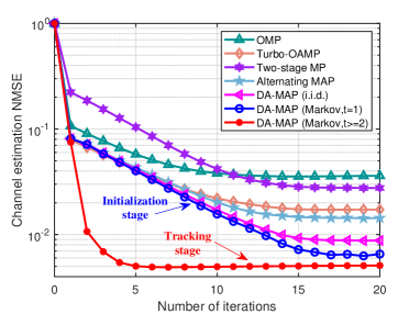
Figure 6: Convergence behavior: NMSE of channel estimation with respect to the number of iterations. ($\textrm{SNR}=5\ \textrm{dB}$)

V-A Convergence Behavior

The convergence behavior of different methods are shown in Fig. 6. As can be seen, the steady-state performance of the proposed method is better than that of baselines. In the channel initialization stage (i.e., $t=1$), there is no prior information for the first frame, and the proposed DA-MAP converges to a good stationary point within $15$ iterations. While in the channel tracking stage (i.e., $t\geq 2$ ), the convergence speed of the DA-MAP is very quick due to the strong prior information passed from the previous frame. In this case, the DA-MAP can converge within $5$ iterations. Besides, the steady-state performance in the tracking stage is better than that in the initialization stage, which reflects that the temporal correlated module in the DA-MAP can not only speed up convergence but also enhance channel tracking performance.

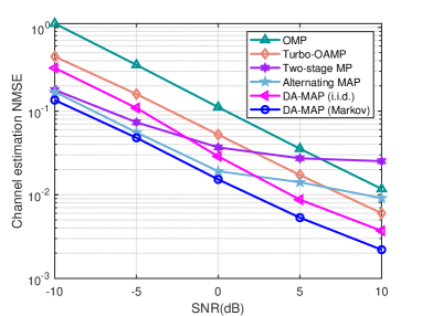
Figure 7: Channel estimation NMSE versus SNR.

V-B Impact of SNR

In Fig. 7, we present the channel estimation NMSE versus SNR. It is obvious that the performance of all the methods improves as SNR increases. However, we find that the channel estimation NMSE of the two-stage MP and alternating MAP decreases slowly in the high SNR regions, while the channel estimation NMSE of other methods decreases linearly with SNR. The main reason is on the VR detection module. Specifically, the two-stage MP performs VR detection based on a coarse estimate of channels, and thus the VR detection error is relatively large. The alternating MAP does not consider the power change effect among visible antennas, and the binary 0/1 VR modeling causes a model mismatch for VRs. In the low SNR regions, the VR detection error is small compared to the noise power. Therefore, the channel estimation NMSE of the two baselines can still decrease linearly with SNR. While in the high SNR regions, the noise power is small. In this case, the VR detection error cannot be neglected and it leads to a relatively poor estimate of channels. In contrast, the OMP and Turbo-OAMP address the VR issue by directly estimating the spatial stationary antenna-delay domain channels. And the proposed DA-MAP can recovery continuous VRs accurately based on the precise VR modeling and efficient algorithm design. Besides, the proposed DA-MAP works better than the OMP and Turbo-OAMP since they cannot exploit the polar-domain sparsity of the XL-MIMO channel. Moreover, the DA-MAP with structured Markov priors achieve a significant performance gain over the DA-MAP with i.i.d. priors, which implies that the temporal correlation of channels and the clustered sparsity of VRs can be exploited to enhance the performance.

Fig. 9 shows the VR estimation NMSE versus SNR. As discussed previously, both the two-stage MP and alternating MAP have a relatively larger VR estimation error than the DA-MAP. Besides, the performance gap between the DA-MAP with Markov priors and the same algorithm with i.i.d. priors is obvious, which means that the proposed hierarchical 2D Markov model can capture the specific sparse structure of VRs.

In Fig. 9, we show the estimated continuous VR over antennas output by different methods, where both the real VR and estimated VR are normalized within the range $\left[0,1\right]$. It can be seen that the two-stage MP and alternating MAP can only detect whether the antenna is visible or not, while the power of visible antennas cannot be recovered. In contrast, the proposed DA-MAP with Markov priors can estimate the power change among visible antennas accurately. When $\textrm{SNR}=5\ \textrm{dB}$, the estimated VR of the DA-MAP with Markov priors is very close to the ground truth.

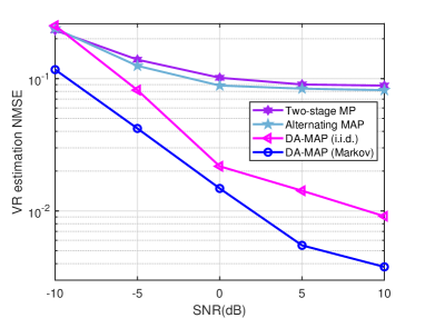
Figure 8: VR estimation NMSE versus SNR.

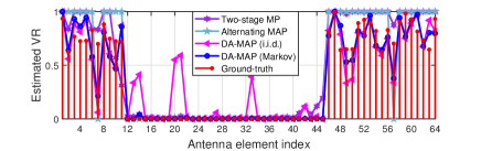
(a) SNR = $-5\ \textrm{dB}$.

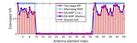
(b) SNR = $5\ \textrm{dB}$.

Figure 9: The power change among visible antennas and the estimated VR of different methods.

V-C Impact of Number of Channel Paths

In Fig. 10, we focus on how the sparsity level of channels affect the channel estimation performance. We change the number of channel paths from $2$ to $10$. As the number of channel paths increases, the performance of all the methods degrades gradually. Again, the proposed DA-MAP with Markov priors achieves the best channel estimation performance.

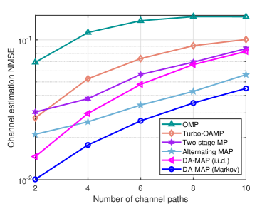
Figure 10: Channel estimation NMSE versus the number of channel paths. SNR is set to $0\ \textrm{dB}$.

V-D Impact of User Speed

In Fig. 11, we study the impact of user speed on the channel estimation NMSE in the tracking stage. When the user speed is high, the scattering environment changes quite quickly. As a result, the convergence speed of the algorithm is slower than the case of low speed. Besides, the steady-state channel tracking performance of the low-speed scenario is better compared to the high-speed scenario. And the performance gap between them is more obvious when SNR is low.

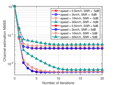
Figure 11: Channel tracking performance of the proposed method under different user speed.

VI Conclusions

We propose a spatial non-stationary channel tracking scheme for XL-MIMO systems with the power change effect. Based on the polar-delay domain sparse representation of XL-MIMO channels, we design a three-layer Markov prior model and a hierarchical 2D Markov model to exploit the dynamic sparsity of channels and VRs over time, respectively. Then, the spatial non-stationary channel tracking problem is formulated as a bilinear measurement process. We develop a novel DA-MAP algorithm to estimate the sparse channel vectors, detect VRs with power change, and refine the polar-delay domain grid. Finally, simulations verified that the proposed DA-MAP outperforms state-of-the-art baselines.

References

- [1] T. S. Rappaport, Y. Xing, O. Kanhere, S. Ju, A. Madanayake, S. Mandal, A. Alkhateeb, and G. C. Trichopoulos, “Wireless communications and applications above 100 GHz: Opportunities and challenges for 6G and beyond,” IEEE Access, vol. 7, pp. 78 729–78 757, 2019.
- [2] H. Lu, Y. Zeng, C. You, Y. Han, J. Zhang, Z. Wang, Z. Dong, S. Jin, C.-X. Wang, T. Jiang, X. You, and R. Zhang, “A tutorial on near-field XL-MIMO communications towards 6G,” IEEE Commun. Surveys Tuts., pp. 1–1, 2024.
- [3] J. Ziniel and P. Schniter, “Dynamic compressive sensing of time-varying signals via approximate message passing,” IEEE Trans. Signal Process., vol. 61, no. 21, pp. 5270–5284, 2013.
- [4] L. Lian, A. Liu, and V. K. N. Lau, “Exploiting dynamic sparsity for downlink FDD-massive MIMO channel tracking,” IEEE Trans. Signal Process., vol. 67, no. 8, pp. 2007–2021, 2019.
- [5] G. Liu, A. Liu, R. Zhang, and M. Zhao, “Angular-domain selective channel tracking and Doppler compensation for high-mobility mmwave massive MIMO,” IEEE Trans. Wireless Commun., vol. 20, no. 5, pp. 2902–2916, 2021.
- [6] Y. Wan and A. Liu, “A two-stage 2D channel extrapolation scheme for TDD 5G NR systems,” IEEE Trans. Wireless Commun., vol. 23, no. 8, pp. 8497–8511, 2024.
- [7] Y. Liu, Z. Wang, J. Xu, C. Ouyang, X. Mu, and R. Schober, “Near-field communications: A tutorial review,” IEEE Open J. Commun. Soc., vol. 4, pp. 1999–2049, 2023.
- [8] M. Cui and L. Dai, “Channel estimation for extremely large-scale MIMO: Far-field or near-field?” IEEE Trans. Commun., vol. 70, no. 4, pp. 2663–2677, 2022.
- [9] E. D. Carvalho, A. Ali, A. Amiri, M. Angjelichinoski, and R. W. Heath, “Non-stationarities in extra-large-scale massive MIMO,” IEEE Wireless Commun., vol. 27, no. 4, pp. 74–80, 2020.
- [10] Z. Yuan, J. Zhang, Y. Ji, G. F. Pedersen, and W. Fan, “Spatial non-stationary near-field channel modeling and validation for massive MIMO systems,” IEEE Trans. Antennas Propag., vol. 71, no. 1, pp. 921–933, 2023.
- [11] Y. Han, S. Jin, C.-K. Wen, and X. Ma, “Channel estimation for extremely large-scale massive MIMO systems,” IEEE Wireless Commun. Lett., vol. 9, no. 5, pp. 633–637, 2020.
- [12] Y. Han, S. Jin, C.-K. Wen, and T. Q. S. Quek, “Localization and channel reconstruction for extra large RIS-assisted massive MIMO systems,” IEEE J. Sel. Topics Signal Process., vol. 16, no. 5, pp. 1011–1025, 2022.
- [13] H. Iimori, T. Takahashi, K. Ishibashi, G. T. F. de Abreu, D. González G., and O. Gonsa, “Joint activity and channel estimation for extra-large MIMO systems,” IEEE Trans. Wireless Commun., vol. 21, no. 9, pp. 7253–7270, 2022.
- [14] Y. Chen and L. Dai, “Non-stationary channel estimation for extremely large-scale MIMO,” IEEE Trans. Wireless Commun., pp. 1–1, 2023.
- [15] Y. Zhu, H. Guo, and V. K. N. Lau, “Bayesian channel estimation in multi-user massive MIMO with extremely large antenna array,” IEEE Trans. Signal Process., vol. 69, pp. 5463–5478, 2021.
- [16] A. Tang, J.-B. Wang, Y. Pan, W. Zhang, X. Zhang, Y. Chen, H. Yu, and R. C. De Lamare, “Joint visibility region and channel estimation for extremely large-scale MIMO systems,” IEEE Trans. Commun., pp. 1–1, 2024.
- [17] W. Xu, A. Liu, M.-j. Zhao, and G. Caire, “Joint visibility region detection and channel estimation for XL-MIMO systems via alternating MAP,” IEEE Trans. Signal Process., vol. 72, pp. 4827–4842, 2024.
- [18] X. Yu, W. Shen, R. Zhang, C. Xing, and T. Q. S. Quek, “Channel estimation for XL-RIS-aided millimeter-wave systems,” IEEE Trans. Commun., vol. 71, no. 9, pp. 5519–5533, 2023.
- [19] W. Xu, Y. Xiao, A. Liu, M. Lei, and M.-J. Zhao, “Joint scattering environment sensing and channel estimation based on non-stationary Markov random field,” IEEE Trans. Wireless Commun., vol. 23, no. 5, pp. 3903–3917, 2024.
- [20] L. Chen, A. Liu, and X. Yuan, “Structured turbo compressed sensing for massive MIMO channel estimation using a Markov prior,” IEEE Trans. Veh. Technol., vol. 67, no. 5, pp. 4635–4639, 2018.
- [21] Z. Lu, Y. Han, S. Jin, and M. Matthaiou, “Near-field localization and channel reconstruction for ELAA systems,” IEEE Trans. Wireless Commun., vol. 23, no. 7, pp. 6938–6953, 2024.
- [22] D. Tse and P. Viswanath, “Fundamentals of wireless communication,” Cambridge University Press, 2005.
- [23] D. Starer and A. Nehorai, “Passive localization of near-field sources by path following,” IEEE Trans. Signal Process., vol. 42, no. 3, pp. 677–680, 1994.
- [24] K. T. Selvan and R. Janaswamy, “Fraunhofer and Fresnel distances: Unified derivation for aperture antennas,” IEEE Antennas Propag. Mag., vol. 59, no. 4, pp. 12–15, 2017.
- [25] Y. Pan, C. Pan, S. Jin, and J. Wang, “RIS-aided near-field localization and channel estimation for the Terahertz system,” IEEE J. Sel. Topics Signal Process., vol. 17, no. 4, pp. 878–892, 2023.
- [26] Z. Yang, L. Xie, and C. Zhang, “Off-grid direction of arrival estimation using sparse Bayesian inference,” IEEE Trans. Signal Process., vol. 61, no. 1, pp. 38–43, 2013.
- [27] L. Xu, L. Cheng, N. Wong, Y.-C. Wu, and H. V. Poor, “Overcoming beam squint in mmwave MIMO channel estimation: A Bayesian multi-band sparsity approach,” IEEE Trans. Signal Process., vol. 72, pp. 1219–1234, 2024.
- [28] M. E. Tipping, “Sparse Bayesian learning and the relevance vector machine,” J. Mach. Learn. Res., vol. 1, no. 3, pp. 211–244, 2001.
- [29] S. Ji, Y. Xue, and L. Carin, “Bayesian compressive sensing,” IEEE Trans. Signal Process., vol. 56, no. 6, pp. 2346–2356, 2008.
- [30] D. G. Tzikas, A. C. Likas, and N. P. Galatsanos, “The variational approximation for Bayesian inference,” IEEE Signal Process. Mag., vol. 25, no. 6, pp. 131–146, 2008.
- [31] L. Cheng, Y.-C. Wu, J. Zhang, and L. Liu, “Subspace identification for DOA estimation in massive/full-dimension MIMO systems: Bad data mitigation and automatic source enumeration,” IEEE Trans. Signal Process., vol. 63, no. 22, pp. 5897–5909, 2015.
- [32] A. Liu, G. Liu, L. Lian, V. K. N. Lau, and M.-J. Zhao, “Robust recovery of structured sparse signals with uncertain sensing matrix: A Turbo-VBI approach,” IEEE Trans. Wireless Commun., vol. 19, no. 5, pp. 3185–3198, 2020.
- [33] E. Fornasini, “2D Markov chains,” Linear Algebra Appl., vol. 140, no. 1, pp. 101–127, 1990.
- [34] F. Kschischang, B. Frey, and H.-A. Loeliger, “Factor graphs and the sum-product algorithm,” IEEE Trans. Inf. Theory, vol. 47, no. 2, pp. 498–519, 2001.
- [35] T. Gao, P. Tang, L. Tian, H. Miao, and Z. Yuan, “A 3GPP-like channel simulation framework considering near-field spatial non-stationary characteristics of massive MIMO,” in Proc. IEEE Globecom, 2023, pp. 1493–1498.