Microscopic imprints of learned solutions in adaptive resistor networks
Abstract
In physical networks trained using supervised learning, physical parameters are adjusted to produce desired responses to inputs. An example is electrical contrastive local learning networks of nodes connected by edges that are resistors that adjust their conductances during training. When an edge conductance changes, it upsets the current balance of every node. In response, physics adjusts the node voltages to minimize the dissipated power. Learning in these systems is therefore a coupled double-optimization process, in which the network descends both a cost landscape in the high-dimensional space of edge conductances, and a physical landscape–the power– in the high-dimensional space of node voltages. Because of this coupling, the physical landscape of a trained network contains information about the learned task. Here we demonstrate that all the physical information relevant to the trained input-output relation can be captured by a susceptibility, an experimentally measurable quantity. We supplement our theoretical results with simulations to show that the susceptibility is positively correlated with functional importance and that we can extract physical insight into how the system performs the task from the conductances of highly susceptible edges.
I Introduction
In artificial neural networks, the cost landscape describes the value of the cost function, , in terms of the parameters, or “adaptable degrees of freedom” [1]. Learned solutions correspond to low minima of this landscape, which are locally described by the cost Hessian [2, 3, 4], the matrix of second derivatives of the cost with respect to the adaptable degrees of freedom, . In the directions of the highest eigenmodes of the cost Hessian, corresponding to the highest positive curvatures, small changes in the adaptable degrees of freedom cause a substantial increase of the cost. These key adaptable degrees of freedom reveal how the system achieves the task; for example, in classification they correspond to the decision boundary [5, 2].
In physical networks, physical parameters such as the stiffnesses or presence of springs connecting nodes in mechanical networks [6, 7, 8, 9, 10], or conductances in resistor networks [11] can be tuned to achieve a desired physical response. In particular, contrastive local learning networks [12, 13], use a local rule [14] rather than gradient descent to adjust their conductances to reach minima in their cost landscapes, enabling them to perform supervised learning without using a processor. Like artificial neural networks, trained physical networks have directions of high curvature in the cost landscape [15] that identify the key adaptable resistors, or key edges, responsible for performing the tasks.
Unlike artificial neural networks, however, these physical networks are also described by a physical landscape. For electrical contrastive local learning networks, this is the dissipated power as a function of all the node voltages, or “physical degrees of freedom” . The response to applied voltages or currents is defined by the minimum of , which translates to Kirchhoff’s current law [16]. The physical landscape for such systems is parabolic and thus fully described by the physical Hessian, the second derivative of the power with respect to the node voltages, .
Learning in electrical resistor networks therefore requires two optimizations. On one hand, the system naturally responds to applied currents/voltages by settling into a voltage configuration that minimizes the power defined by the edge conductances. On the other hand, the system adjusts the edge conductances, modifying the power landscape and response, to minimize the cost function. This double optimization leaves strong signatures in the physical modes for generic Hopfield [17], elastic [18, 19, 20, 21, 17], and flow/resistor networks [22, 17]. These signatures include low-dimensional physical responses and alignment of low-lying eigenmodes with the functional response [17]. Most notably, stiff eigenmodes of the cost Hessian are related to soft eigenmodes of the physical Hessian [15]: for a task in which an applied voltage drop across one edge leads to an equal voltage drop across another edge, the lowest physical mode and the highest cost mode contain the same information [15]. In this case, the lowest eigenmode of the physical Hessian tells us the key edges, namely the edges that are most responsible for performing the task. For more complex tasks, however, the situation is not as simple. Here we show precisely how much information about the cost Hessian is contained in the physical Hessian for arbitrarily complex tasks.
Our results provide a general way of identifying the key edges from physical properties of the networks alone. We demonstrate how this identification can be used to gain physical insight into the inner workings of trained networks–something that is not possible in artificial neural networks.
II Systems Studied
We will couch our analysis in the language of adaptable resistor networks of nodes and edges, in which each edge corresponds to a linear resistor with adjustable conductance. Each node in the network is characterized by a voltage with respect to a ground. Each edge connecting two nodes and carries a current proportional to the voltage difference, , with being the conductance of the edge connecting nodes and . Throughout the article we reserve indices to indicate nodes and to indicate edges. We use vectors to describe voltage states , conductance states , and current states .
For the numerical analyses, we use adaptable resistor networks of size nodes obtained from jammed packings, as in previous studies [23, 11]. Inspired by real laboratory implementations, we constrain edge conductances to lie within a finite but wide range of . We train the networks using Coupled Learning [11], but emphasize that our theoretical results are independent of the training process. The main assumption is that the cost is near the global minimum value of zero, so the task has been learned. For training details, initial conditions, and hyperparameters of the different examples shown in the paper, see Appendix D.
III Relation between the cost and physical Hessians
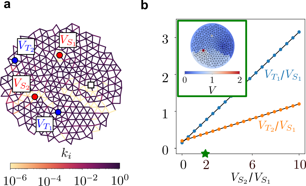
The following derivation holds for any trained task. However, it is useful to have in mind an illustrative example. As such an example, consider a network trained for a linear regression task, fig. 1. The network has two source nodes and , and two target nodes and , satisfying the following relation:
| (1) |
In addition, we hold a node at ground voltage (Fig. 1a), as in experiments. This removes the trivial zero modes of the physical landscape corresponding to uniform shifts of voltage on all the nodes. The physical Hessian for a grounded linear resistor network is given by
| (2) |
where is the incidence matrix, the diagonal matrix of conductances, and is a canonical vector with entry 1 at the fixed ground node . This extended Hessian or bordered Laplacian [15, 23] removes the trivial zero mode of the network, allowing the physical Hessian to be inverted, . Under this formulation, the voltage configuration is extended with the current (Lagrange multiplier) needed to ground the system, .
Additional external input currents associated e.g. with training samples, can be generically encoded into a current vector of the form , where the last entry corresponds to the value corresponding to the ground voltage. The system’s voltage response to all of the applied currents must minimize the dissipated power
| (3) |
leading to,
| (4) |
Supervised learning corresponds to modifying the response to a given set of inputs to satisfy constraints . Usually, these constraints act on specific nodes designated as output voltage nodes. Denoting the projector onto these output nodes for task , each constraint can be written as
| (5) |
where is the vector of desired output values for the intputs . Notice that the length of and is equal to the number of output nodes.
The cost is then naturally defined as the sum of the squared constraints over the tasks the networks is being trained, corresponding to the mean squared error (MSE):
| (6) |
Under the assumption that all the constraints are satisfied at the end of training, , the cost Hessian reads [15]:
| (7) |
Using Eqs. (5) and (4), we carry out the derivatives of the constraints over the voltage response,
| (8) |
leading to
| (9) |
This expression highlights two contributions to the cost Hessian. First, there is a physical contribution stemming from . This contribution is agnostic to training details and therefore depends only on the conductance values and the network topology. Second, there is a training contribution that depends on how the system is trained, namely the identities of the output nodes embodied in , and the input values for each task, .
We can explicitly separate physical and training contributions of the cost Hessian by employing higher-order tensors. Denoting the outer product with , we define the 4th-rank training tensor and the 4th-rank susceptibility tensor as
| (10) | ||||
| (11) |
from which we can express the cost Hessian as the full contraction of these last two tensors:
| (12) |
Equation (12) clearly establishes that the susceptibility tensor contains all the physical information of the cost Hessian. Its components measure the sensitivity of the inverse of the physical Hessian (the response) to changes in conductances. Notably, the entries of this tensor are modified by the training components , yet they do not depend explicitly on them. We highlight that while the derivation of Eq. (12) assumed the MSE as the cost function, eq. (6), this result is valid for any form of cost provided it is differentiable and has a minimum, see Appendix A.
In what follows we provide a simpler analytical expression of the susceptibility tensor and link it to the linear response of the system.
IV The susceptibility tensor
Using Eq. (2) and the derivative of the matrix inverse, we explicitly compute the derivatives of the inverse physical Hessian appearing in Eq. (11):
| (13) |
where is vector formed by the -th row of the incidence matrix . For clarity we define the extended vector (bold font) by adding an extra zero, and the susceptibility vector as
| (14) |
corresponding to a vector of dimensions defined per edge . Under this notation, the derivative of the inverse physical Hessian reads
| (15) |
yielding the final expression for the susceptibility tensor:
| (16) |
At this point, the power dependence of both Hessians becomes evident. Eq. (14) explicitly shows that the susceptibility vector scales as the inverse of the physical Hessian, . Applying this scaling relation four times, as per eq. (16), we obtain , and ultimately .
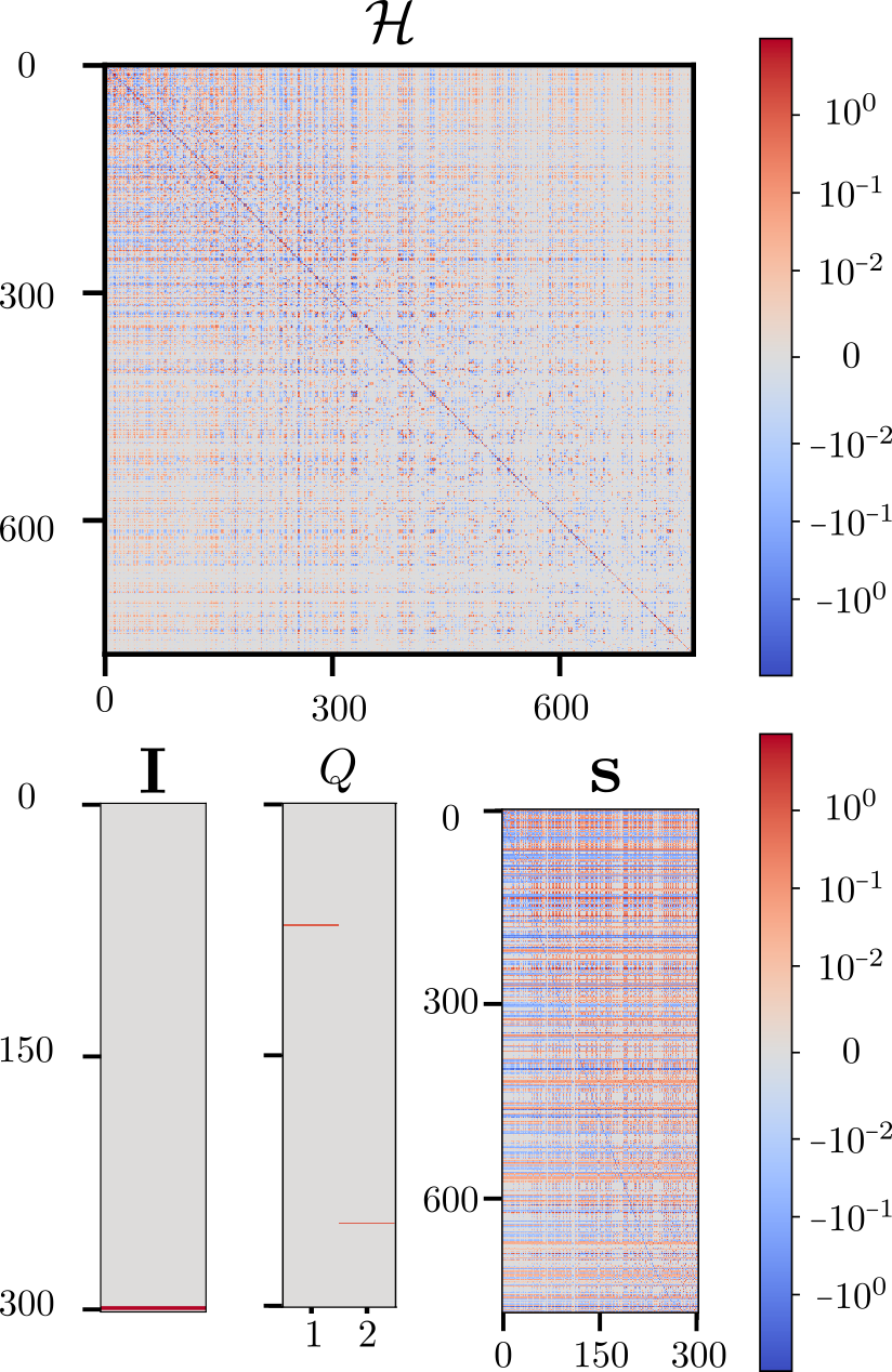
While each entry is a 4th rank tensor, rendering a 6th order tensor, its components are all determined by the susceptibility vectors defined per edge. Moreover, the susceptibility vectors are dense as opposed to the sparse nature of the input currents and the projectors , fig. 2. Simply put, the larger the susceptibility , the larger the entry , which, on average and depending on the training tensor , tends to manifest as large entries of the cost Hessian . We thus turn our attention to the susceptibility vectors and their norms.
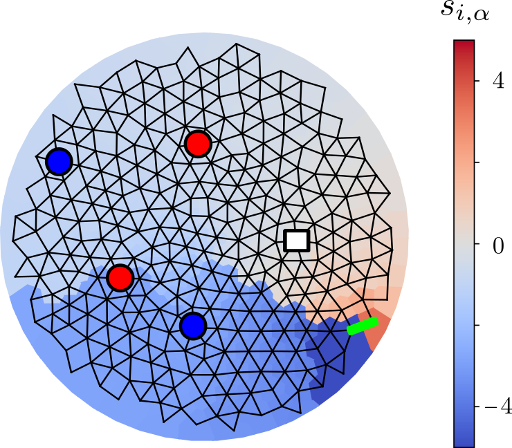
The definition of is directly related to the response of the system. Contracting it with an input current , it leads to voltage drop at edge of the physical response to the current ,
| (17) |
Thus each element is the voltage drop at edge of the response to a unit current at node , fig. 3. The magnitude of quantifies the voltage drop linked to all possible unit currents in the network and assigns a scalar measure of susceptibility per edge:
| (18) |
Denoting by and the eigenvalues and normalized eigenvectors of the physical Hessian, , we can recast the susceptibility as
| (19) |
with norm
| (20) |
where we have used the orthonormality of the eigenvectors . Equation (20) shows that the magnitude of the susceptibility is dominated by soft modes (small ). Thus, edges with large susceptibility must have large voltage drops across the modes, specially the softest.
In summary, we have demonstrated that all the physical information of the cost Hessian boils down to the dense susceptibility tensor and ultimately to the susceptibility vectors . The susceptibilities are dominated by soft modes of the physical Hessian with large voltage drops, and correlate positively with the cost Hessian.
These results, although written in the language of resistor networks, are far more general. There are only three necessary conditions to derive Eqs. (12) and (16):
-
I.
The adaptable degrees of freedom satisfy all the constraints and therefore (eq. (6)). In other words, the system has been trained successfully.
-
II.
The physical response to externally applied inputs minimizes a scalar function with respect to the physical degrees of freedom, . In other words, the physical system optimizes a Lyapunov function.
-
III.
The response to inputs is approximated by the perturbations around a known local minimum of , .
In low Reynolds number flow networks, the adaptable degrees of freedom may correspond to pipe diameters, the physical degrees of freedom to node pressures, and the scalar function to the power dissipated. In elastic networks, the adaptable degrees of freedom may taken to be the stiffness or rest lengths of all of the springs, the physical degrees of freedom are the node positions or displacements, and is the elastic energy or free energy.
Conditions II and III allow for a generic perturbative description of nonlinear physical landscapes in terms of the closest local minimum to the response . In such case, eq. (3) becomes , with a nonlinear function of the physical degrees of freedom . To second order,
| (21) |
where the physical Hessian is given by . Then, the response is given by , and the same derivations ensue from eq. (5).
In the remainder of the paper, we work exclusively with resistor networks to elucidate the physical significance of highly-susceptible edges. Since they capture much of the information of the cost Hessian, we delve into how much they contribute to its stiff modes. Recall that stiff directions in the cost landscape correspond to directions in which the cost is particularly sensitive to changes of parameters (adaptable degrees of freedom).
In the next sections we analyze three different learning tasks, previously implemented in experimental networks [12, 13], and demonstrate that the susceptibility is highly correlated with stiff modes of the cost Hessian, and therefore to the degree of sensitivity of the cost to the adaptable degrees of freedom corresponding to those directions in the cost landscape. Finally, we will connect the susceptibility to the low-dimensional response observed in trained networks [17] and the topological nature of the response in allosteric networks [24].
V Stiff modes and susceptible edges
The description of the cost landscape near the solution is fully encoded in the cost Hessian . Its eigenvalues, , and eigenvectors , describe the curvature along different directions. Figure 4a shows the distribution of eigenvalues before and after training. Before training, the network has a wide distribution of cost eigenvalues and a non-zero cost gradient. After training, the spectrum is highly degenerate. Most of the eigenvalues are close to zero while four are very high. The same behavior has been observed in artificial neural networks [2, 3]. The modes with high eigenvalues, or stiff modes, correspond to the number of coefficients learned by the linear regression task (details in fig. 1). The entries of each of the stiff modes measure the importance of the given edge to the function (Fig. 4b). Perturbing any of those edges amounts to moving in conductance space along, at least partially, directions of high-curvature, substantially increasing the cost .
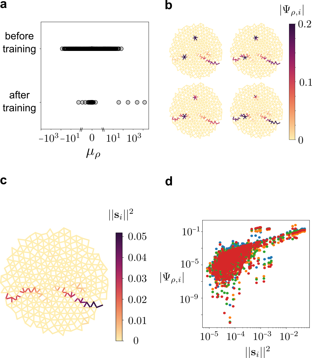
Remarkably, the scalar field of the norm of susceptibilities shown in Fig. 4c reveals the same patterns as we see in the stiff modes, Fig. 4b. In Fig. 4d we quantify this observation with a correlation scatter plot over the edges of the network, showing that high-susceptibility correlate strongly with large entries of the stiff modes.
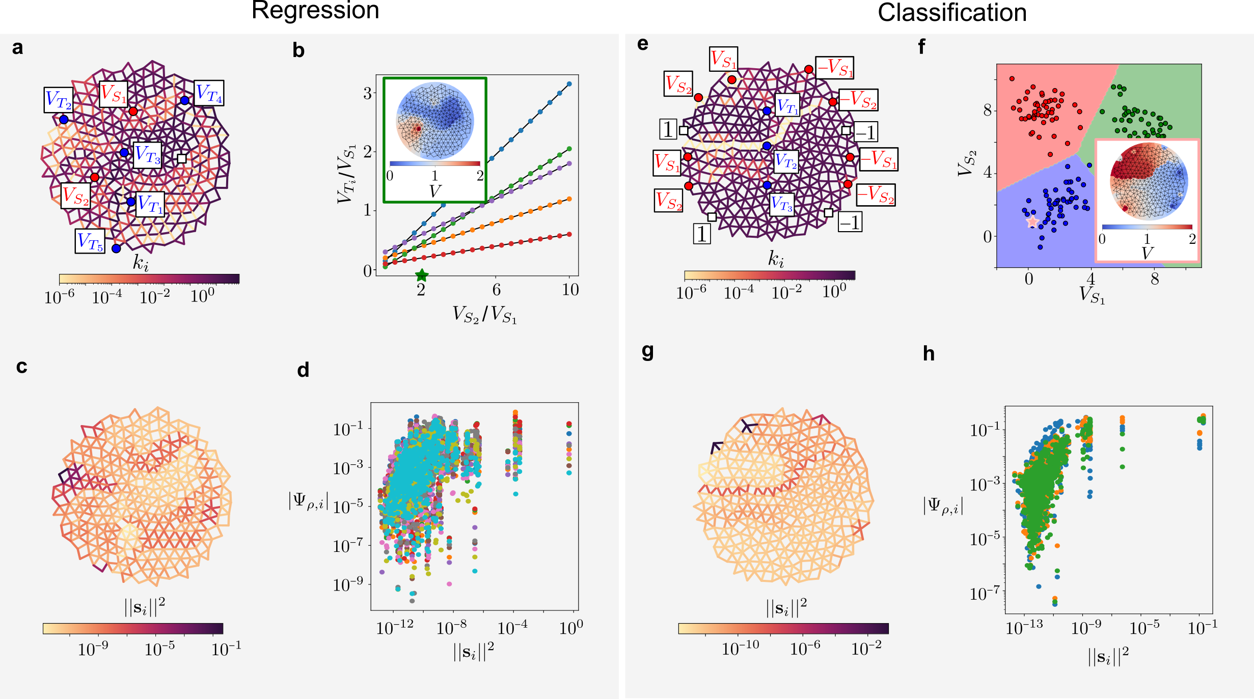
Regression: a. Conductance configuration of a network trained for the five target linear regression task specified by the coefficients in (22). Source nodes are denoted by red circles, target nodes by blue circles and the grounded node by a white square. b. The ratio of the voltage at each of the target nodes with respect to the voltage source (circles) obeys the required linear dependence (solid lines). Inset: voltage response associated to the green star ( and ). c. Scalar field of , with darker colors indicating larger susceptibilities. d. The edges of higher susceptibility positively correlate with the entries of the 10 stiffest modes of the network. Classification: Same panels as before for a network trained to classify three classes of data as shown in f, where the inset corresponds to the the voltage response to the inputs indicated by the pink star.
We illustrate the strong correlation between edge susceptibility and stiff modes of the cost Hessian for three more tasks. First we consider a more complicated linear regression task, consisting of two input and 5 output nodes. The vector of desired voltages as a function of input voltages is given by
| (22) |
where as before, a ground node is kept at zero voltage, making all the linear relations non-colinear.
The network is trained down to a cost of , ending up with a set of conductances that satisfies the task, Fig. 5a and b. As with the previous linear regression task, high susceptibility edges positively correlate with those singled out from stiff modes, fig. 5c and d,
A more stringent test corresponds to linear classification. Here we train the network to classify three different classes depending on two input voltages, fig. 5e and f. We encode the corresponding classes with three output nodes. To convert classification into a numerical task, we use “one-hot encoding” for each output node. For example, a point belonging to class 2, corresponds to . For this case, a more suitable cost function corresponds to the cosine similarity:
| (23) |
where corresponds to the cosine of the angle between the two vectors.
This is a significantly harder task for the network to achieve for three reasons. First, the physical restriction of having positive conductances only allows for decision boundaries with positive slope. To overcome this, we represent each input value as two different and opposite voltage nodes, Fig. 5e. We do the same for the ground nodes, placing one low (-1) and high (+1) ground. Second, the two-dimensional embedding of the network topologically constraints current flows, leading to output nodes being effectively isolated from input nodes. We solve this by doubling the information and copying each input node twice, as well as the low and high grounds. Third, achieving perfect one-hot encoding is impossible for a linear resistor network, since it corresponds to a highly non-linear output as a function of the input voltages. Nevertheless, we can still train and interpret the result using a winner-take-all strategy, in which the network classifies according to the maximum target value, . Figure. 5f shows that the network trains successfully, finding a set of edge conductances that leads to a classification accuracy of . Even though the training and task are more involved, the susceptibility vector is a good proxy of the stiff modes, as shown in fig. 5g and h.
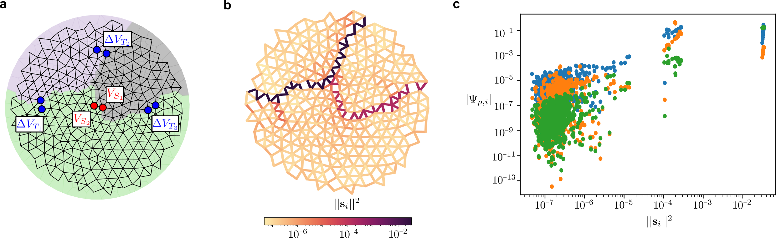
V.1 Connection to persistent homology
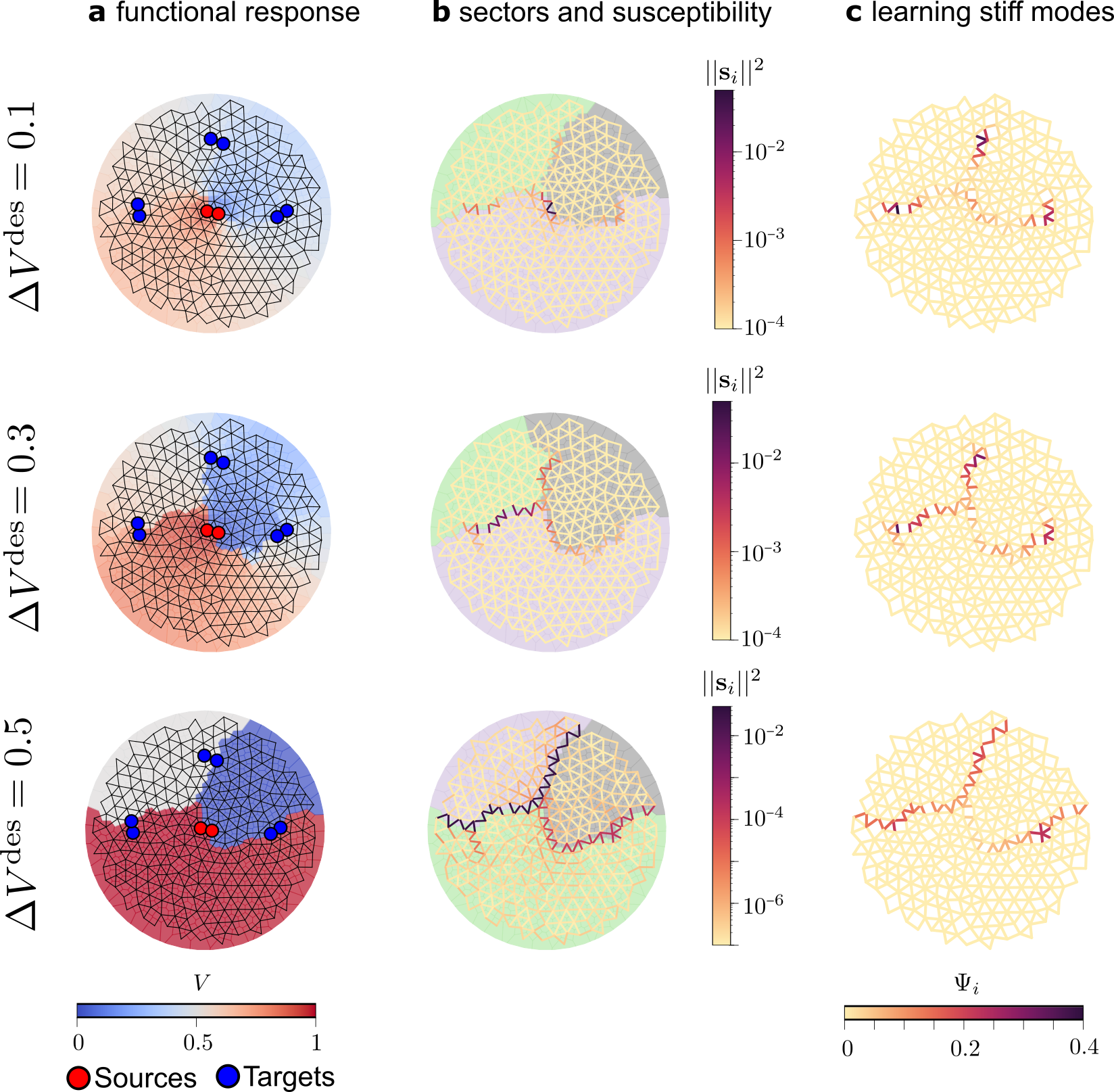
As a last family of examples, we analyze networks trained to provide specified voltage drops across output edges in response to a voltage drop across an input edge [23] (Fig. 6a). Such long-range effects require precise values of the conductances in resistor or flow networks [23]. Compared to the previous regression and classification tasks, this task is significantly simpler due to the fixed input values it is trained on. One of the remarkable results for networks trained for such tasks is that the response is topological in structure [24, 25, 26]. Regardless of the values the networks is trained on, the response of the system tends to partition into sectors of roughly homogeneous voltages, captured by a topological data analysis approach known as persistent homology, as shown in Fig. 6a [25, 24]. It turns out that the boundaries of the topological sectors are precisely the edges with large susceptibility (Fig. 6b). These also correspond to edges singled out by stiff modes of the cost Hessian (Fig. 6c). In Appendix B, we show that the susceptibility is even better at capturing the important edges for weak training signals.
VI Low-dimensional response
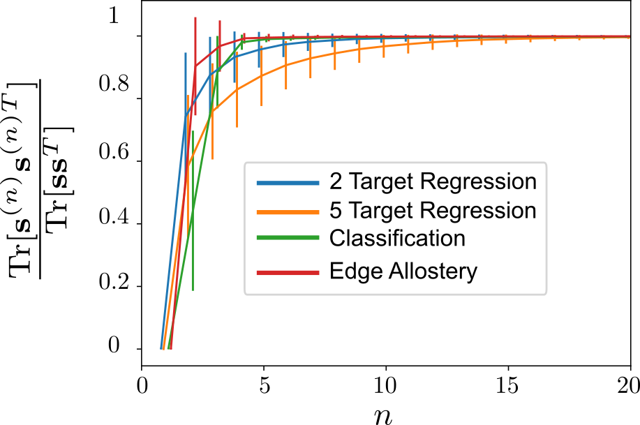
One of the hallmarks of physical learning in linear networks is the low dimensionality of the physical response [27]. Mechanical and resistor networks have been shown to exhibit trained responses that depend only on a handful of physical soft modes, representing a small fraction of all the modes. This low dimensionality is also suggested by the susceptibility norm in Eq. (20): the mode contributions decay with increasing magnitude of the eigenvalues. We explore the dimensionality reduction by determining the number of modes required to define the susceptibility norm. We define the partial susceptibility as
| (24) |
Clearly, we recover the full susceptibility when , i.e. the total number of modes. Figure 7 shows the norm of the partial susceptibility as a function of the number of modes for all four cases studied in the paper. Aligned with the dimensionality reduction of trained responses, for all cases the norm saturates at values ranging from to , showing that most of the physical information is encoded in a few soft modes.
VII Physical interpretation of role of key edges
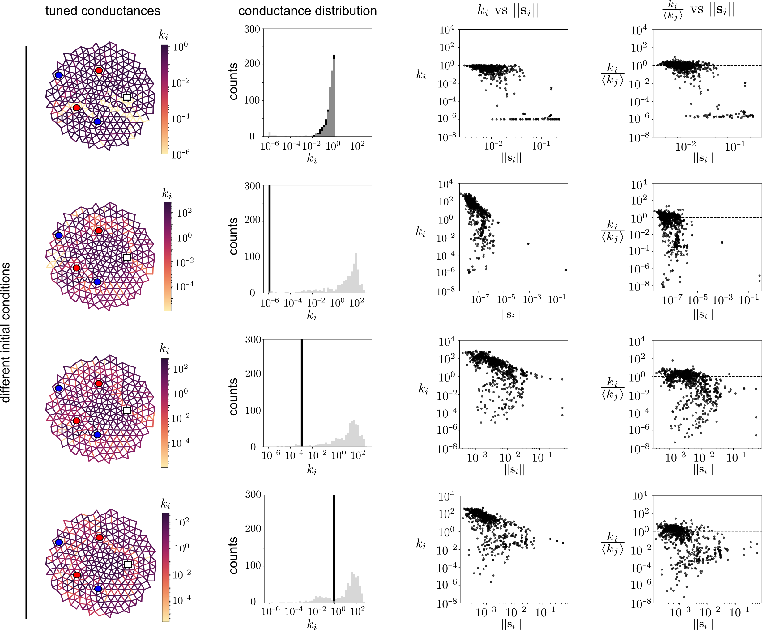
We have established that the susceptibility, a physical quantity devoid of learning information, correlates positively with the stiff modes of the cost Hessian. Highly-susceptible edges are therefore important for the functionality of the network. But how do highly-susceptible edges affect the physical response? We next study the conductance values of the trained networks and analyze them in relation to their susceptibility values.
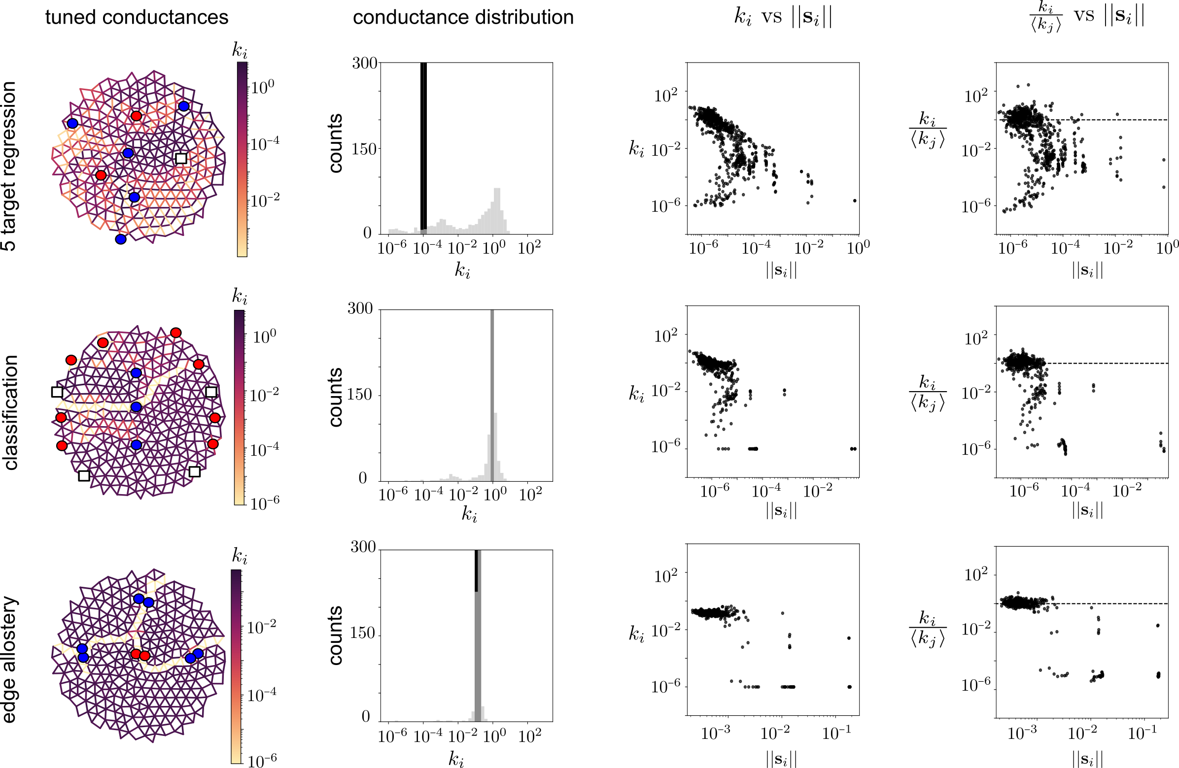
We consider the linear regression task of Fig. 1 with four sets of random initial conditions: uniformly-distributed between and and sharper distributions peaked at , , and . The results are shown in fig. 8: Different initial configurations lead to qualitatively different final states, each of them performing exactly the same task. The existence of multiple good solutions is a signature of the overparameterization of the networks (first column and second column). With the exception of the first example (first row), conductance is generically not correlated with the susceptibility (third column). This observations also holds for all the examples analyzed presented in the main text (see Appendix C). The fourth column shows the relation between the relative conductance of each edge with its susceptibility , where is the average conductance of the adjacent edges. While their relation depends on the task and initial condition, one striking feature is common across all the examples: high-susceptibility edges have low relative conductances , (see Appendix C) for more examples). We highlight that this does not need to be the case, as one can imagine a functional network relying on connected segments of very high conductance (pipelines) to accomplish the same task. The training procedure we use (Coupled Learning) does not appear to generically yield such solutions; how different training protocols might affect the nature of trained solutions is an interesting subject for further study.
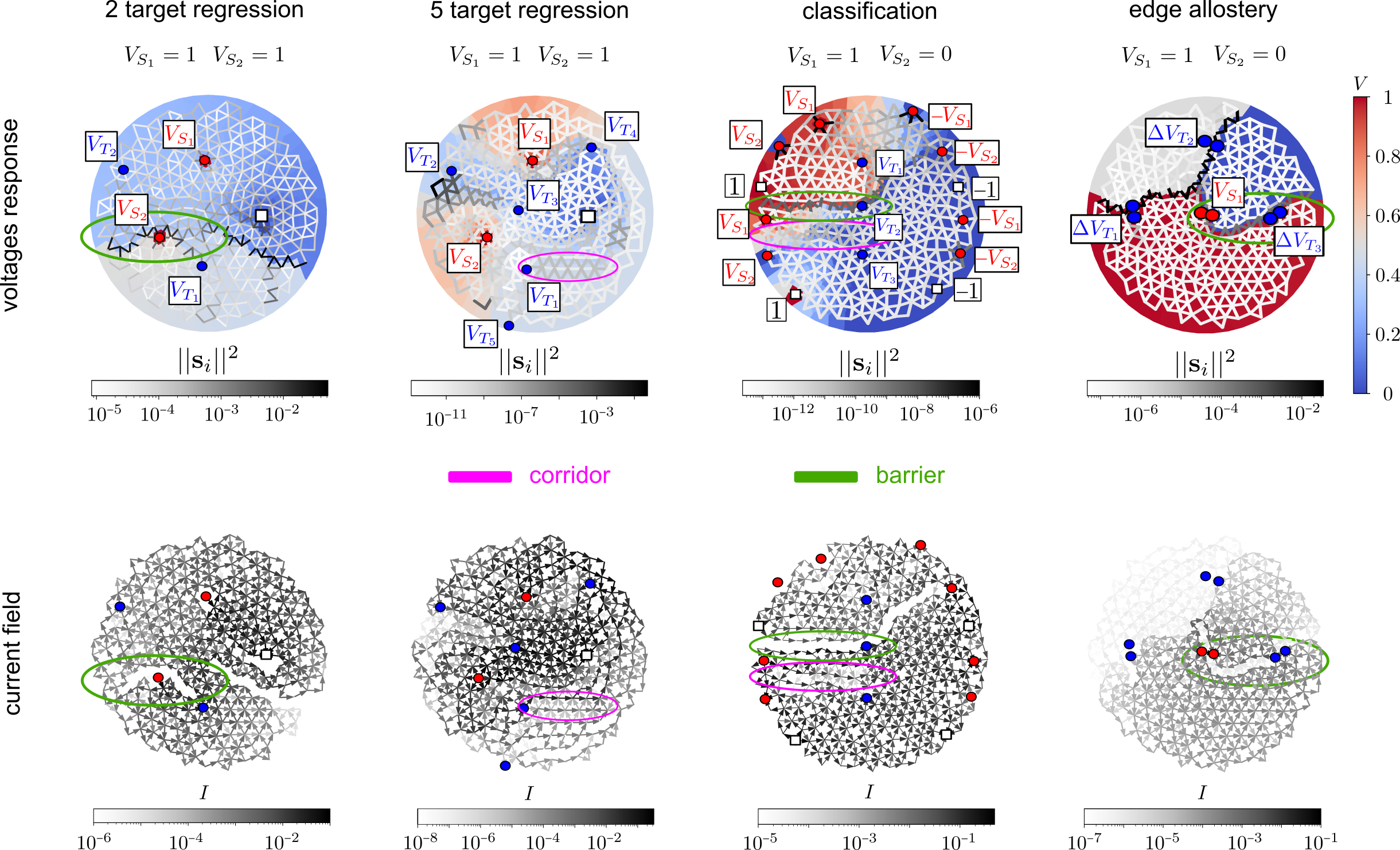
In Fig. 9 we illustrate how edges with high susceptibility and low relative conductance effectively act as current blockers, or barriers, for generic input voltages. We analyze the four tasks of the main text: linear regression with two targets, with five targets, classification, and trained voltage drops at output edges (different columns). The first row illustrates the voltage response (background color) for given input voltages and highly susceptible edges (gray scale). The current field, shown in the second row, shows how current flows from inputs to outputs in the network. Highly-susceptible edges block the current along them, redirecting it by at least two identifiable mechanisms: acting as a wall to concentrate voltage on either side (highlighted in green), or forming corridors through which the current is concentrated and routed to specific locations (highlighted in pink).
The system places walls and corridors to accomplish the trained task. Take, for example, the linear regression task for two targets (first row). A wall separates nodes from but not . This is a sensible strategy because is nearly equally distant from both and but was trained for a dependence on that is only half as strong as the dependence on (see eq. (1)). Similar conclusions can be drawn for the other tasks (Appendix C). These results show that the joint information of susceptibility and conductance can provide physical insight into how the systems accomplish their tasks.
VIII Discussion
Trained resistor networks have their learned solutions imprinted into their physical landscapes. We have shown that the local geometry of the cost landscape around the learned solution, characterized by the cost Hessian, stems from two separable quantities. The first is the training tensor, , which depends solely on the task the system has been trained to perform: the location of input and output nodes, and the input currents corresponding to the training samples. The second quantity is the susceptibility tensor , which depends solely on physical properties of the network, namely its architecture and the edge conductances.
The explicit decoupling of training (task-dependent) and physical quantities has several consequences. First, it extends and formalizes the correspondence between cost and physical Hessians [15], allowing us to extract the key, highly-susceptible edges. The key edges are those indicated by the stiff modes of the cost Hessian, and are the most important edges for performing the task. Here we have shown that they tend to have high susceptibilities, so that they can be identified from physical properties of the network alone, without needing to know the task.
Second, it establishes a fundamental bound on the physical information contained in the cost Hessian. For linear resistor networks, all the physical information is encoded in the susceptibility tensor. For nonlinear networks, all of the physical information up to quadratic order in the physical landscape is encoded in the susceptibility tensor.
We have shown that the susceptibility tensor , which can be decomposed into susceptibility vectors , explains previous observations on physical learning such as the low-dimensional response [17], the mode correspondence in simple tasks [15], and the topological structure of allosteric networks [24].
Third, it provides an experimentally measurable quantity independent of the training details. Measurements such as the response to localized input currents can be used to extract , revealing critical information about how the task is performed.
In short, the double optimization at the heart of physical learning in many systems makes it possible to gain physical insight into how trained tasks are accomplished. Such insight does not exist for artificial neural networks, which do not possess a physical landscape.
While all the derivations were explicitly done in the context of resistor networks, the same results naturally extend to elastic networks, where the response minimizes energy, and in general, to any physical network that minimizes a scalar quantity (a Lyapunov function) and whose response can be approximated by a physical Hessian around a known minimum.
As an example, elastic networks have been trained to have responses similar to protein allostery, in which strain applied by binding one molecule affects the ability of a second type of molecule to bind to the protein elsewhere. Spring networks have been trained to develop allosteric responses using global gradient descent [6], Monte Carlo methods [19, 28], or local learning rules such as directed aging [29] and Coupled Learning [11]. By contrast, real proteins have been trained to perform allostery via biological evolution. The generality of our theoretical analysis implies that it may be applied independent of the process by which a system developed the ability to perform a task. This generality suggests that the connection [21] between slow physical modes of proteins and underlying nonlinearities that correlate non-pairwise additive effects of mutations of amino acids in the sequence (global epistasis) can be generalized to gain physical insight into global epistasis even in cases where allostery is not characterized by a single slow mode.
Furthermore, our methods should yield potentially useful insight into how proteins perform allosteric tasks. Using persistent homology, a topological data analysis tool, it has been shown that the functional response of trained allosteric networks can often be described by robust macroscopic sectors highlighting large-scale structures in the network [26] akin to functional regions observed in allosteric proteins [30]. The persistent homology analysis depends on both training (input nodes and values) and physical (response) information. We have shown that similar topological structures can be obtained with physical information alone, through the susceptibility tensor, in a closely related system. An important direction for future work is to apply our analysis to mechanical networks with allostery to extract key edges and compare to persistent homology results.
More generally, our results pave the way towards understanding and interpreting how collective trained behavior emerges. Here we have studied linear networks, for which the physical landscape is completely convex and possesses only one minimum. Biological, physical, and artificial systems, however, heavily rely on non-linearities to achieve more and more complex tasks [31, 28, 8, 32, 33]. This is the case, for example, of elastic networks with multistable allostery [28] and also resistor networks that learn non-linear regression and classification [13, 34]. For such systems, the physical landscape is decorated with several minima, with each minimum characterized by different susceptibilities. Understanding how distributions and correlations among edge susceptibilities might vary among minima is an important area of future work, akin to the study of statistical comparisons of the properties of different jammed minima in sphere packings [35].
IX Acknowledgements
This work was supported by DOE Basic Energy Sciences through grant DE-SC0020963 (MG,FM,MS), the UPenn NSF NRT DGE-2152205 (FM) and the Simons Foundation through Investigator grant #327939 to AJL. MS was also supported by NIH CRCNS grant 1R01MH125544-01 and NSF grant CISE 2212519.
Appendix A - decomposition for general cost functions
The cost function can be written as
| (25) |
where are generic (non-linear) differentiable constraints depending on the voltages at the output nodes, . For fully trained networks, , and the cost hessian is given by
| (26) |
where,
| (27) |
and is the derivative of the constraint with respect to its arguments evaluated at the output voltage nodes. In the case of the MSE cost used in the main text, this last term is equal to a vector of ones.
Using the last two equations, we can write the cost hessian as
| (28) |
which can be again be split into a learning and susceptibility tensor :
| (29) |
with
| (30) | ||||
| (31) |
As expected, the susceptibility tensor is not modified by the specifics of the cost function.
Appendix B Comparison between persistent sectors and susceptibility in allosteric networks
Here we provide further evidence that the sectors obtained by persistence homology in allosteric networks are readily captured by the pattern of susceptibilities, and that they correspond to the stiff modes of the cost hessian. We consider the same task as in the main text: two inputs nodes with voltages 0 and 1, and three target edges trained for the same voltage drop value . In addition to the original task shown in fig. 6 (), we consider two more subtle cases: and , which require much less training but leave weaker imprints into the cost hessian. The voltage response field shows sharper variations as increases, fig. 11a, leading to clear partitions, or sectors, captured by persistent homology [25], fig. 11b. As decreases, the susceptible edges have a smaller overlap with the boundaries of the persistent sectors, yet they accurately capture the stiff modes of the cost hessian, fig. 11c. For details of the persistent homology algorithm see [25].
Appendix C Susceptibilities and conductances of remaining examples
In figure 10 we show the distribution of conductances and edge susceptibilities for the circuits in figures 5a, 5e, and 6. For all these cases, the same general features mentioned in the main text hold: high-susceptible edges generically have low relative conductances, while the conductance itself is not indicative of the susceptibility values.
Appendix D Training protocol
All the networks were trained using Coupled Learning [27], a contrastive local learning rule with two hyperparameters: the learning rate and the nudge parameter (for details of the training scheme, see [27]).
The first linear regression circuit (fig. 1) was trained for iterations, each iteration batching 30 training samples, using , , and initial conductances drawn from a uniform distribution in , reaching a final MSE cost .
The input data consisted of 112 pairs of voltages with corresponding outputs given by the linear relation of eq. (1).
The second linear regression circuit (fig. 5a) was trained for iterations, each iteration batching 30 training samples, using , , and initial conductances drawn from a uniform distribution in , reaching a final MSE cost . The input data consisted of 112 pairs of voltages with corresponding outputs given by the linear relation of eq. (22).
The classification circuit (fig. 5e) was trained for iterations, each iteration batching 30 training samples, using , , and initial conductances all equal to , reaching a final cosine similarity cost , train accuracy of (120 points), and test accuracy of (30 points). The input data consisted of three clusters of points, one per class, generated from the following normal distributions:
| (32) | |||
| (33) | |||
| (34) |
The allosteric circuit (fig. 6) was trained for iterations, no batching, using , , and initial conductances were drawn from a uniform distribution in , reaching a final MSE cost . The input data is , with corresponding output . The additional two allosteric circuits in fig. 11 were trained for iterations, no batching, using , and initial conductances were drawn from a uniform distribution in , reaching final MSE costs of () and ().
Appendix E Susceptibility for weakly trained networks
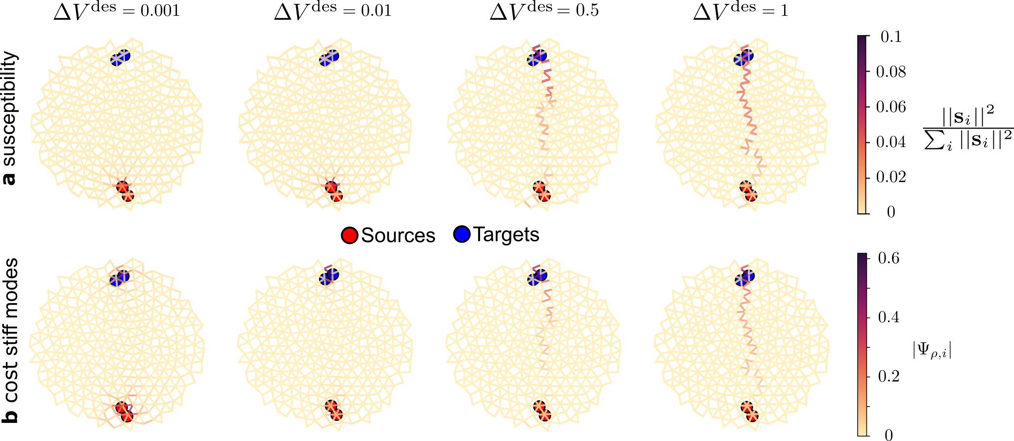
Figure 12 shows how the susceptibility depends on the task strength. We consider an allosteric task with two input voltages (0 and 1), and one edge target with increasing desired voltage drop . The lower the desired voltage drop, the easier the task and less training steps are required. In fig. 12 we show that despite the weak signals, the susceptibilities still capture the relevant edges highlighted by the stiff mode of the cost hessian.
References
- Mehta et al. [2019] P. Mehta, M. Bukov, C.-H. Wang, A. G. Day, C. Richardson, C. K. Fisher, and D. J. Schwab, A high-bias, low-variance introduction to machine learning for physicists, Physics reports (2019).
- Sagun et al. [2016] L. Sagun, L. Bottou, and Y. LeCun, Eigenvalues of the hessian in deep learning: Singularity and beyond, arXiv preprint arXiv:1611.07476 (2016).
- Sagun et al. [2017] L. Sagun, U. Evci, V. U. Guney, Y. Dauphin, and L. Bottou, Empirical analysis of the hessian of over-parametrized neural networks, arXiv preprint arXiv:1706.04454 (2017).
- Dauphin et al. [2014] Y. N. Dauphin, R. Pascanu, C. Gulcehre, K. Cho, S. Ganguli, and Y. Bengio, Identifying and attacking the saddle point problem in high-dimensional non-convex optimization, Advances in neural information processing systems 27 (2014).
- Sabanayagam et al. [2023] M. Sabanayagam, F. Behrens, U. Adomaityte, and A. Dawid, Unveiling the hessian’s connection to the decision boundary, arXiv preprint arXiv:2306.07104 (2023).
- Rocks et al. [2017] J. W. Rocks, N. Pashine, I. Bischofberger, C. P. Goodrich, A. J. Liu, and S. R. Nagel, Designing allostery-inspired response in mechanical networks, Proceedings of the National Academy of Sciences 114, 2520 (2017).
- Pinson et al. [2017] M. B. Pinson, M. Stern, A. Carruthers Ferrero, T. A. Witten, E. Chen, and A. Murugan, Self-folding origami at any energy scale, Nature communications 8, 15477 (2017).
- Hexner et al. [2020a] D. Hexner, N. Pashine, A. J. Liu, and S. R. Nagel, Effect of directed aging on nonlinear elasticity and memory formation in a material, Physical Review Research 2, 043231 (2020a).
- Pashine [2021] N. Pashine, Local rules for fabricating allosteric networks, Physical Review Materials 5, 065607 (2021).
- Arinze et al. [2023] C. Arinze, M. Stern, S. R. Nagel, and A. Murugan, Learning to self-fold at a bifurcation, Phys. Rev. E 107, 025001 (2023).
- Stern et al. [2021] M. Stern, D. Hexner, J. W. Rocks, and A. J. Liu, Supervised learning in physical networks: From machine learning to learning machines, Physical Review X 11, 021045 (2021).
- Dillavou et al. [2022] S. Dillavou, M. Stern, A. J. Liu, and D. J. Durian, Demonstration of decentralized physics-driven learning, Physical Review Applied 18, 014040 (2022).
- Dillavou et al. [2024] S. Dillavou, B. D. Beyer, M. Stern, A. J. Liu, M. Z. Miskin, and D. J. Durian, Machine learning without a processor: Emergent learning in a nonlinear analog network, Proceedings of the National Academy of Sciences 121, e2319718121 (2024).
- Stern and Murugan [2023] M. Stern and A. Murugan, Learning without neurons in physical systems, Annual Review of Condensed Matter Physics 14, 417 (2023).
- Stern et al. [2024a] M. Stern, M. Guzman, F. Martins, A. J. Liu, and V. Balasubramanian, Physical networks become what they learn, arXiv preprint arXiv:2406.09689 (2024a).
- Vadlamani et al. [2020] S. K. Vadlamani, T. P. Xiao, and E. Yablonovitch, Physics successfully implements lagrange multiplier optimization, Proceedings of the National Academy of Sciences 117, 26639 (2020).
- Stern et al. [2024b] M. Stern, A. J. Liu, and V. Balasubramanian, Physical effects of learning, Physical Review E 109, 024311 (2024b).
- Tlusty et al. [2017] T. Tlusty, A. Libchaber, and J.-P. Eckmann, Physical model of the genotype-to-phenotype map of proteins, Physical Review X 7, 021037 (2017).
- Yan et al. [2017] L. Yan, R. Ravasio, C. Brito, and M. Wyart, Architecture and coevolution of allosteric materials, Proceedings of the National Academy of Sciences 114, 2526 (2017).
- Yan et al. [2018] L. Yan, R. Ravasio, C. Brito, and M. Wyart, Principles for optimal cooperativity in allosteric materials, Biophysical Journal 114, 2787 (2018).
- Husain and Murugan [2020] K. Husain and A. Murugan, Physical constraints on epistasis, Molecular Biology and Evolution 37, 2865 (2020).
- Anisetti et al. [2023] V. R. Anisetti, A. Kandala, and J. Schwarz, Emergent learning in physical systems as feedback-based aging in a glassy landscape, arXiv preprint arXiv:2309.04382 (2023).
- Rocks et al. [2019] J. W. Rocks, H. Ronellenfitsch, A. J. Liu, S. R. Nagel, and E. Katifori, Limits of multifunctionality in tunable networks, Proceedings of the National Academy of Sciences 116, 2506 (2019).
- Rocks et al. [2020] J. W. Rocks, A. J. Liu, and E. Katifori, Revealing structure-function relationships in functional flow networks via persistent homology, Physical Review Research 2, 10.1103/physrevresearch.2.033234 (2020).
- Rocks et al. [2021] J. W. Rocks, A. J. Liu, and E. Katifori, Hidden topological structure of flow network functionality, Physical Review Letters 126, 028102 (2021).
- Rocks et al. [2024] J. W. Rocks, E. Katifori, and A. J. Liu, Topological characterization of the continuum of allosteric response, arXiv preprint arXiv:2401.13861 (2024).
- Stern et al. [2022] M. Stern, S. Dillavou, M. Z. Miskin, D. J. Durian, and A. J. Liu, Physical learning beyond the quasistatic limit, Phys. Rev. Research 4, L022037 (2022).
- Rouviere et al. [2023] E. Rouviere, R. Ranganathan, and O. Rivoire, Emergence of single-versus multi-state allostery, PRX Life 1, 023004 (2023).
- Hexner et al. [2020b] D. Hexner, A. J. Liu, and S. R. Nagel, Periodic training of creeping solids, Proceedings of the National Academy of Sciences 117, 31690 (2020b).
- Halabi et al. [2009] N. Halabi, O. Rivoire, S. Leibler, and R. Ranganathan, Protein sectors: Evolutionary units of three-dimensional structure, Cell , 774 (2009).
- Alim et al. [2017] K. Alim, N. Andrew, A. Pringle, and M. P. Brenner, Mechanism of signal propagation in physarum polycephalum, Proceedings of the National Academy of Sciences 114, 5136 (2017).
- Anisetti et al. [2022] V. R. Anisetti, A. Kandala, B. Scellier, and J. Schwarz, Frequency propagation: Multi-mechanism learning in nonlinear physical networks, arXiv preprint arXiv:2208.08862 (2022).
- Hornik et al. [1989] K. Hornik, M. Stinchcombe, and H. White, Multilayer feedforward networks are universal approximators, Neural networks 2, 359 (1989).
- Stern et al. [2024c] M. Stern, S. Dillavou, D. Jayaraman, D. J. Durian, and A. J. Liu, Training self-learning circuits for power-efficient solutions, APL Machine Learning 2 (2024c).
- Liu and Nagel [2010] A. J. Liu and S. R. Nagel, The jamming transition and the marginally jammed solid, Annu. Rev. Condens. Matter Phys. 1, 347 (2010).