Quantum-Inspired Weight-Constrained Neural Network: Reducing Variable Numbers by 100x Compared to Standard Neural Networks

Abstract

Although quantum machine learning has shown great promise, the practical application of quantum computers remains constrained in the noisy intermediate-scale quantum era. To take advantage of quantum machine learning, we investigate the underlying mathematical principles of these quantum models and adapt them to classical machine learning frameworks. Specifically, we develop a classical weight-constrained neural network that generates weights based on quantum-inspired insights. We find that this approach can reduce the number of variables in a classical neural network by a factor of 135 while preserving its learnability. In addition, we develop a dropout method to enhance the robustness of quantum machine learning models, which are highly susceptible to adversarial attacks. This technique can also be applied to improve the adversarial resilience of the classical weight-constrained neural network, which is essential for industry applications, such as self-driving vehicles. Our work offers a novel approach to reduce the complexity of large classical neural networks, addressing a critical challenge in machine learning.

Introduction

Large artificial intelligence (AI) models are transforming our education and research, enabling groundbreaking advances in various domains [1, 2, 3, 4, 5, 6]. For example, OpenAI’s GPT series and Google’s BERT have revolutionized our ability to generate human-like texts, recognize complex image patterns, and interpret audio [7]. Similarly, AlphaFold has simplified the design and discovery of new proteins and drugs [8, 9]. The remarkable capabilities of these large AI models arise from their vast networks, often containing billions or even trillions of variables [10]. However, the large scale of these AI models induces many significant challenges, including high memory requirements, overfitting, convergence difficulties, and complex hyperparameter tuning [11, 12]. Addressing these challenges requires the development of AI models that could maintain strong learnability while reducing the complexity of the models.

Emerging quantum machine learning techniques offer promising solutions to some challenges posed by large AI models [13, 14, 15, 16, 17, 18]. The advantage of quantum speed-ups has been demonstrated in various machine learning tasks [14, 19], including finding concise functions to fit exponentially large datasets [20], learning a particular data distribution [18], discovering unknown kernel functions [21], and extracting insights from experimental data points using exponentially fewer data compared to classical approaches [22]. These advances can significantly reduce the computational time required to train AI models. Beyond speed, quantum machine learning offers memory advantages by taking advantage of the exponential storage capability of quantum computers. For example, quantum neural networks with amplitude encoding require far fewer variables than their classical counterparts [23]. Consequently, the vast number of parameters in large AI models can be effectively reduced by employing quantum or hybrid quantum-classical models.

Driven by these advantages, quantum machine learning (QML) has become an active area of research [24, 25, 26, 27, 28, 29, 30, 31, 32, 33, 34]. Although substantial progress has been made in the development of QML algorithms, there are still few real-world applications that leverage real quantum computers [35, 36, 37, 38, 39]. This gap largely results from the quantum noise issue, which prevents reliable results when many qubits are used [40, 41]. Addressing this noise challenge is complex, and achieving a large-scale, noise-free quantum computer is expected to take considerable time. In light of these obstacles, the development of quantum-inspired classical algorithms that address the challenges of classical machine learning is a valuable direction to advance machine learning techniques [42, 43, 44, 45, 46, 47, 48].

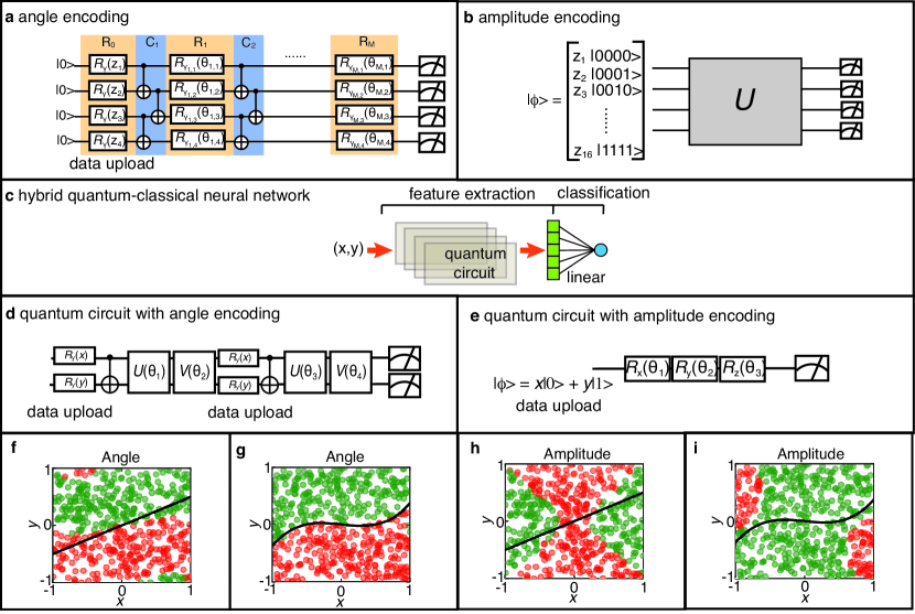
Figure 1: Hybrid quantum-classical neural network. a A generic quantum circuit with angle encoding. b A generic quantum circuit with amplitude encoding. c A hybrid quantum-classical neural network. d A two-qubit quantum circuit using angle encoding. The operators $U$ and $V$ are illustrated in supplementary note 1. e A one-qubit quantum circuit using amplitude encoding. f Training result of the hybrid network with angle encoding for classifying whether a data point lies above or below the boundary $y=x/2$, shown as a black line. The green color denotes the predicted value above the boundary, while the red indicates the prediction below the boundary. g Training result of the hybrid network with angle encoding for classifying whether a data point lies above or below the boundary $y=x(x-0.5)(x+0.5)/2$. h Training result of the hybrid network with amplitude encoding, addressing the same task as in panel f. i Training result of the hybrid network with amplitude encoding, addressing the same task as in panel$\bf g$.

In this work, we present a method to reduce the number of variables in classical deep-learning neural networks by drawing inspiration from quantum neural networks that employ angle and amplitude encodings. Our analysis reveals that using a parameterized quantum circuit with angle encoding is mathematically equivalent to constructing a polynomial function, where each term is expressed as a continuous product of the cosine series components [47]. In contrast, a quantum circuit with amplitude encoding is designed to establish correlations between elements in the input data. We note that the number of variables in the correlation matrix is determined by the number of parameterized gates rather than the dimensionality of the input data, implying that the quantum circuit with amplitude encoding needs fewer variables compared to the classical neural network. These insights motivate us to develop an algorithm capable of generating thousands of weights using only dozens of variables. Specifically, we utilize a combinatorial approach to create numerous sets of angle combinations. Each combination is then used to construct weights through the continuous product of trigonometric functions. We validate this weight-constrained method by examining its performance on four datasets: MNIST, Fashion MNIST, CIFAR, and traffic datasets. Our results demonstrate that the weight-constrained method maintains the learnability of the classical neural network while substantially reducing the number of variables. This approach holds promise for scaling down variable numbers in large AI models such as GPT and BERT. Furthermore, we develop a novel method to enhance the adversarial resilience of the quantum neural network and the classical weight-constrained neural network models by randomly dropping parameterized angles during prediction. We demonstrate that such a method can significantly increase resilience against adversarial attacks.

Quantum neural networks

To develop quantum-inspired classical neural networks, we explore the underlying mathematics of quantum neural networks with angle and amplitude encodings [1]. In this work, we elucidate how these two types of quantum neural networks select features. After building on this mathematical foundation, we develop a quantum-inspired classical neural network, which utilizes 100 times fewer variables than a standard classical neural network.

Quantum neural network with angle encoding

We start to analyze the quantum neural network with angle encoding, which adopts the input value as rotation angles in the quantum gates, as shown in Fig. 1a. The nonlinear relationship between the output of a quantum circuit and the input data ${\bf z}$ is constructed by applying different rotation gates and CNOT gates in this circuit. Without loss of generality, we consider a quantum circuit shown in Fig. 1a, which has one data-upload layer $\tilde{R}_{0}$, $M$ rotation layers, and $M$ CNOT layers. The rotation operator $R_{\gamma}$ in Fig. 1a is chosen from the group $\{R_{x},R_{y},R_{z}\}$. Then, the final quantum state of this quantum circuit is

$$|\psi\rangle=\tilde{R}_{M}\tilde{C}_{M}\cdots\tilde{R}_{1}\tilde{C}_{1}\tilde{R}_{0}|0000\rangle,$$ (1)

where $\tilde{R}_{i}$ denotes a matrix constructed from the tensor product of different single-gate rotation matrices within one layer, and $\tilde{C}_{i}$ denotes a matrix constructed from the tensor product of two-gate CNOT matrices. If we adopt measurements $A$ with Pauli operators, it is straightforward to find that the output $O$ of a quantum circuit is a polynomial function, which is expressed as

$$O = \langle\psi|A|\psi\rangle=\sum_{s}f_{s}({\bf\theta},{\bf z}),$$ (2)

$$f_{s}({\bf\theta},{\bf z}) = c_{s}\prod_{i}\mathrm{cos}(\theta_{i}/2+q_{i})\prod_{j}\mathrm{cos}(\theta_{j}/2+q_{j})\times$$ (3)

$$\prod_{n}\mathrm{cos}(z_{n}/2+q_{n})\prod_{m}\mathrm{cos}(z_{m}/2+q_{m}),$$

where $c_{s}$ belongs to {$1,-1$}. The symbol $q_{i}$ denotes $0$ or $\pi/2$. Equation (2) shows that the quantum neural network with angle encoding creates a complicated activation function, which could select features better than the classical activation functions, such as ReLU and Tanh. We refer the reader to our previous work [47] for a deeper understanding of this quantum activation function.

Quantum neural network with amplitude encoding

Unlike angle encoding, which transforms real-world data into rotation angles, amplitude encoding transforms real-world data into coefficients of pure quantum states. For the amplitude encoding, the initial state of a quantum circuit $|\phi\rangle$ is set as

$$|\phi\rangle_{i}=\frac{z_{i}}{|{\bf z}|}|b_{i}\rangle,$$ (4)

where $|b_{i}\rangle$ denotes a pure quantum state, i.e., $|0000\rangle$ and $|0001\rangle$. $|{\bf z}|$ is the norm value of the input vector ${\bf z}$. This initial quantum state can be transformed to other states by applying rotation and CNOT gates. For simplicity, we can use an operator $U$ to represent these operations as shown in Fig. 1b. Then, the final quantum state is written as

$$|\psi\rangle=U|\phi\rangle.$$ (5)

If we set the measurement operator as $A$, the output $O$ of this quantum circuit is

$$O=\langle\phi|U^{\dagger}AU|\phi\rangle=\langle\phi|W|\phi\rangle,$$ (6)

where $W$ is a unitary matrix. It is easy to rewrite Eq. (6) as

$$O=\frac{1}{|{\bf z}|^{2}}\sum_{i,j}z_{i}W_{ij}z_{j}.$$ (7)

We can eliminate the factor $\frac{1}{|{\bf z}|^{2}}$ because it is equivalent to data normalization. A key observation from Eq. (7) is that the quantum circuit creates a correlation matrix between any two elements in the input data. For example, $W_{1,2}$ represents the correlation between the first and second input features, and $W_{1,100}$ denotes the correlation between the first and the one hundredth input features. If all elements in $W$ are nonzero, the construction of features incorporates long-range and short-range correlations[21]. It is important to emphasize that the quantum convolutional neural network proposed in Ref. 49, which applies convolutional operations between neighboring qubits, inherently creates long-range entanglement among real-world input features. This characteristic fundamentally differentiates the feature selection in the quantum convolutional neural network from that in the classical convolutional neural network, as the latter typically relies on spatially localized filters.

The quantum neural network (QNN) with amplitude encoding inherently limits the nonlinear relationship between input and output to a quadratic order, regardless of the complexity of the quantum circuit. This constraint makes it challenging for the QNN with amplitude encoding to extract features that involve three-point or four-point correlations. In contrast, a QNN with angle encoding can more effectively capture these higher-order correlations, as shown in Eq. (2). To illustrate this limitation, we consider the task of identifying whether a data point is above or below a boundary.

Figure 1c shows a hybrid quantum-classical neural network (HNN) that we adopt to perform the task, classifying whether a data point is above or below a boundary. In this setup, the quantum circuit is responsible for feature constructions, while a fully connected classical neural network with a linear activation function performs the classification. The quantum circuits for angle encoding and amplitude encoding are depicted in Figs. 1d and 1e, respectively. The two-qubit operators $U$ and $V$ are sketched in supplementary note 1. As shown in Figs. 1f-1i, we evaluate the performance of the hybrid network on two different boundaries: $y_{1}=x/2$ and $y_{2}=x(x-0.5)(x+0.5)/2$, using angle and amplitude encodings. The black curve denotes the boundary, the green dot denotes the predicted value above the boundary, and the red dot denotes the predicted value below the boundary. The QNN with amplitude encoding struggles to identify both boundaries because the features derived from terms like $x^{2}$, $xy$, and $y^{2}$ are insufficient to characterize $y_{1}$ and $y_{2}$. However, the QNN with angle encoding successfully identifies the boundary for $y_{2}$ due to its ability to capture the third-order term (i.e., $x^{3}$) inherent in the problem. The higher-order term can be obtained from the Taylor expansion of the cosine function. The subpar performance of angle encoding for $y_{1}$ can be attributed to the excessive nonlinearity imposed by the QNN.

Although QNNs with amplitude encoding exhibit lower learnability compared to those with angle encoding, they offer a key advantage: the ability to represent large datasets using relatively few qubits, thereby requiring fewer variables. This benefit is reflected in the substantially reduced number of variables in the weight matrix $W$ shown in Eq. (7). In other words, the weight elements in $W$ are not independent, and the variable number of the weight matrix is determined by the number of rotation angles rather than the dimensionality of the matrix. This observation suggests that independent weights $W_{ij}$ may not be necessary for classical deep-learning neural networks.

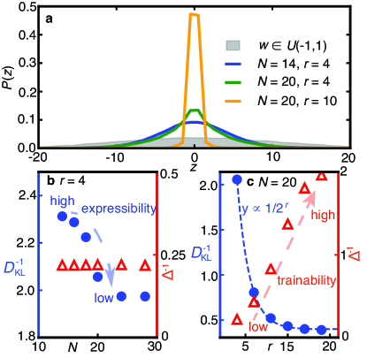
Figure 2: The expressibility and trainability of a neural network using the weight-constrained method. a The distribution $P(z)$ of $z$, defined as $z=\sum_{i}w_{i}x_{i}$, where $w$ denotes the weight, and $x$ denotes the input features. b The inverse of Kullback-Leibler divergence $D_{\text{KL}}^{-1}$ as a function of $N$, where $N$ denotes the number of variables. The right axis shows the inverse of the standard derivation $\Delta^{-1}$. c The inverse of Kullback-Leibler divergence $D_{\text{KL}}^{-1}$ as a function of $r$, where $r$ denotes the number of variables that are selected from $N$ variables. The blue dashed line represents a fitted curve.

Quantum-inspired classical network: weight-constrained neural network

By exploring quantum neural networks with angle and amplitude encodings, we find the underlying mathematical principles of these two quantum models. Our key finding reveals that the weight elements in quantum neural networks are determined by parametric rotation angles through trigonometric functions. Building on this insight, we develop a classical weight-constrained neural network.

In the classical weight-constrained neural network, we construct weight variables as follows. To generate $K$ different weights, we first define $N$ different variables, denoted as $\theta$. Then a combination process is performed, where $r$ variables are chosen from these $N$ variables, resulting in $C(N,r)$ possible combinations. Labeling the $k$-th combination as ${\bf\theta}^{(k)}$, the $k$-th weight $w_{k}$ is defined as

$$w_{k}=\prod_{i\in\mathrm{even},i\leq r}\mathrm{cos}(\theta_{i}^{(k)})\prod_{j\in\mathrm{odd},j\leq r}\mathrm{sin}(\theta_{j}^{(k)}).$$ (8)

This combination strategy enables constructing thousands of weights using only a few dozen variables. We note that the weight correlation at the first moment is zero because

$$\int_{-\pi}^{\pi}d{\bf\theta}w_{k}w_{k^{\prime}}=2^{N-r}\pi^{N}\delta_{k,k^{\prime}}.$$ (9)

In addition, these weights are always correlated in higher moments, that is

$$\int_{-\pi}^{\pi}d\theta w_{k}^{s}w_{k}^{\prime,s}\neq 0,$$ (10)

when $s>1$.

When the weight-constrained method is applied to a classical neural network, it reduces the learnability of the network, which refers to the ability to learn a target function. To investigate the impact of this constraint on learnability, we examine two distinct two-layer neural networks. In the first classical network, 1000 input features, $x$, are connected to an output neuron, $y$, as follows:

$$y = f(z),$$ (11)

$$z = \sum_{i}w_{i}x_{i}$$ (12)

where $w_{i}$ represents the weight, sampled from the uniform distribution $U(-1,1)$. Here, $f(z)$ denotes a standard classical activation function, such as Tanh, Sigmoid, or ReLU. The second classical neural network has the same architecture as the first. However, in the second network, weights are determined using the weight-constrained method described in Eq. (8). Notably, the uniformly distributed bias term affects the distribution of $z$ in the same way for both networks and is therefore omitted from this analysis.

Figure 2a displays the distribution $P(z)$ of $z$ for both classical neural networks. The input features $x$ are sampled from a uniform distribution $U(-1,1)$. The gray shading represents the distribution for the classical neural network with weights sampled from $w\in U(-1,1)$. The colored curves correspond to the classical weight-constrained neural network for various values of $N$ and $r$, which are parameters used to construct the combination sets. As shown in Fig. 2a, both networks exhibit dome-shaped distributions centered at $z=0$. Including a uniformly distributed bias term does not affect the central position of these distributions. It is observed that the weight-constrained network displays a narrower distribution width and a more pronounced peak compared to the network with uniformly distributed weights. This result suggests that the weight-constrained method limits access to larger $z$ values, thereby reducing the learnability of the network. When the activation function is applied to $z$, the weight-constrained method impacts the expressibility of different activation functions differently. For example, the weight-constrained method has a smaller effect on the Tanh function compared to the ReLU function because larger values of $|z|$ are less essential for the Tanh function. Further details on this observation can be found in Supplementary Note 3.

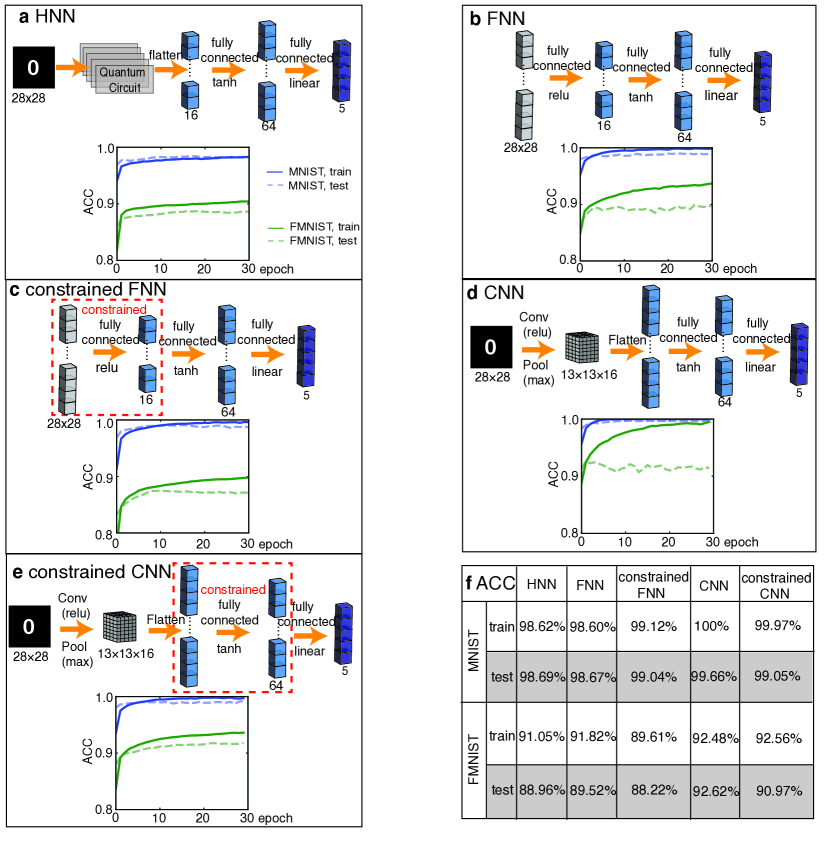
Figure 3: Training results of different neural networks. a The architecture of the hybrid quantum-classical neuron network (HNN) and the training results on the MNIST and Fashion MNIST (FMNIST) datasets. Here, ACC denotes accuracy. b The fully connected neuron network (FNN) architecture and the training results on the MNIST and FMNIST datasets. c The weight-constrained FNN architecture and the training results on the MNIST and FMNIST datasets. d The convolutional neural network (CNN) architecture and the training results on the MNIST and FMNIST datasets. e The architecture of the weight-constrained CNN and the training results on the MNIST and FMNIST datasets. f A summary of the ACC of these five models for MNIST and FMNIST datasets.

To quantify the reduction in learnability caused by the weight-constrained method, we employ the Kullback–Leibler divergence ($D_{\text{KL}}$), defined as

$$D_{\text{KL}}=\sum_{z}p(z)\log\left(\frac{p(z)}{q(z)}\right),$$ (13)

where $p(z)$ represents the distribution of $z$ for the network using the weight-constrained method, and $q(z)$ represents the distribution for the network with uniformly distributed weights. The value of $D_{\text{KL}}$ is inversely proportional to the expressibility of the network; thus, a higher expressibility corresponds to a larger $D^{-1}_{\text{KL}}$ [50].

Figures 2b and 2c depict the inverse of the Kullback–Leibler divergence ($D^{-1}_{\text{KL}}$, blue circles) as a function of $N$ (at $r=4$) and $r$ (at $N=20$), respectively. The result shows that the increase in $N$ or $r$ reduces the value of $D^{-1}_{\text{KL}}$, indicating a reduction in expressibility. Notably, the expressibility declines more rapidly with increasing $r$ compared to increasing $N$. Using a fitting approach, we find that $D^{-1}_{\text{KL}}$ decays as a function of $1/2^{r}$, which is shown as the blue dashed curve in Fig. 2c. This result highlights the importance of selecting a small value of $r$ to preserve strong expressibility.

For the Tanh and Sigmoid activation functions, the output $y$ exhibits a larger slope when $z$ is near zero, but the slope approaches zero for $|z|>2$. A larger slope generally indicates better trainability. To assess the trainability of the network using the weight-constrained method, we examine the standard deviation $\Delta$ of the distribution $p(z)$, represented by the red triangular symbols in Figures 2b and 2c. At $r=4$, $\Delta^{-1}$ is nearly constant with varying $N$, indicating that changes in $N$ do not significantly impact trainability. In contrast, $\Delta^{-1}$ shows a linear dependence but not an exponential dependence on $r$, implying that the phenomenon of quantum barren plateaus [51] is absent in the classical weight-constrained neural network. Moreover, the result in Fig. 2c indicates that the weight-constrained network with larger values of $r$ exhibits higher trainability. However, given the reduced expressibility at large $r$, it is crucial to optimize $r$ to balance expressibility and trainability. It is worth noting that these trainability analyses do not apply to the ReLU activation function because the slope for $z>0$ is independent of the value of $z$.

Practicality of the weight-constrained method

Having discussed the expressibility and trainability of classical neural networks employing the weight-constrained method, we now focus on its practical applications in classical fully connected and convolutional neural networks.

We begin by comparing the performance of the classical weight-constrained neural network with that of a standard classical fully connected neural network (FNN) and a hybrid neural network (HNN). The architectures of these three networks are depicted in Figs. 3a- 3c, respectively. All three networks consist of four layers, with 16 neurons in the first hidden layer and 64 neurons in the second hidden layer. Details on the quantum circuit design are provided in Supplementary Note 1. For the weight-constrained FNN, the weights in the first hidden layer are determined using Eq.(8). In addition to FNN, we evaluate the performance of the classical weight-constrained convolutional neural network (CNN) and its standard counterpart. Figure 3d illustrates a standard CNN architecture comprising one convolutional layer, one pooling layer, and two fully connected layers. The weight-constrained CNN, shown in Fig. 3e, shares the same architecture as the standard CNN, but the weight-constrained method is applied to the first fully connected layer.

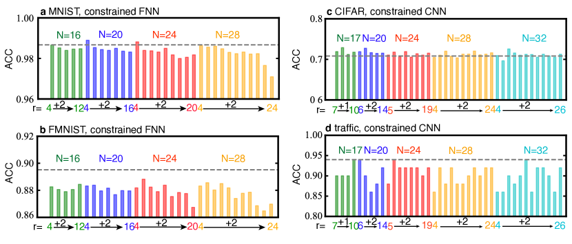
Figure 4: The accuracy (ACC) of the weight-constrained fully connected neural network (FNN) and the weight-constrained convolutional neural network (CNN) for different values of $N$ and $r$. The ACC refers to the accuracy of the test dataset. Here, $N$ and $r$ represent variables in the combination formula $C(N,r)$. Panel a and panel b plot the results of the MNIST and the FMNIST datasets. Panel c and panel d plot the results of the CIFAR and the traffic datasets. The gray dashed line denotes the ACC of the standard neural network.

We first train HNN, FNN, and weight-constrained FNN on the MNIST and Fashion MNIST (FMNIST) datasets (see details in the Methods section). In the HNN, each quantum circuit comprises 38 variables. The combination sets in the weight-constrained FNN are formed by selecting five elements from a pool of 15 variables. The table in Fig. 3f summarizes the optimal results of these networks, determined based on the minimal loss function for the test datasets. For the MNIST test dataset, the HNN and the FNN achieved similar accuracies (ACC) of 98.7%, which is 0.3% smaller than the ACC of the weight-constrained FNN. For the FMNIST test dataset, the HNN and the FNN performed comparably, achieving an ACC of 89%, approximately 1% larger than that of the weight-constrained FNN. These results demonstrate that although the weight-constrained FNN reduces the number of variables by a factor of 52, its learnability is not significantly suppressed.

Next, we train the CNN and the weight-constrained CNN on these two datasets. In the weight-constrained CNN, the weight-constrained method is implemented by selecting five elements from a pool of 20 variables, reducing the number of variables by a factor of 135 compared to the standard CNN. Despite this substantial reduction in variables, the table in Fig. 3f shows that the weight-constrained CNN achieves an ACC comparable to the standard CNN on the MNIST test dataset. For the FMNIST test dataset, the ACC of the weight-constrained CNN is only 1.65% smaller than that of the standard CNN. Notably, the difference between training and test accuracies at a large epoch (i.e., 30) is smaller for the weight-constrained CNN and the weight-constrained FNN compared to their standard counterparts. This observation suggests that the weight-constrained method effectively mitigates overfitting. This advantage arises from the limited learnability of the weight-constrained neural network, which filters out noise in the training data while retaining essential signals.

To further investigate the impact of the combination method in the weight-constrained strategy, we perform simulations using different values of $N$ and $r$. Figure 4 presents the ACC for the MNIST, FMNIST, CIFAR, and traffic test datasets. In these simulations, the weight-constrained FNN is applied to the MNIST and FMNIST datasets, whereas the weight-constrained CNN is used for the CIFAR and traffic datasets. The gray dashed line represents the ACCs of their respective classical standard counterparts. For each pair of $(N,r)$, the displayed result reflects the optimal outcomes of 16 independent simulations. For weight-constrained FNN, the ACC generally decreases as $r$ increases, which is attributed to the lower expressibility of the network at large $r$ values. Furthermore, ACC does not show a significant dependence on the value of $N$, consistent with the small change of $D_{\mathrm{KL}}^{-1}$ induced by $N$ shown in Fig. 2b. This result suggests that decreasing $r$ is more critical than decreasing $N$ to achieve better performance.

The performance of the weight-constrained neural network, compared to the standard classical neural network, varies depending on the characteristics of the dataset. For example, the weight-constrained FNN achieves a larger ACC on the MNIST dataset compared to the standard FNN, but it exhibits 1% smaller ACC on the FMNIST dataset. The weight-constrained CNN achieves a comparable or larger ACC on the CIFAR and traffic datasets relative to the standard CNN, while its ACC for the FMNIST test dataset is 1% smaller (see Supplementary Note 3 for details). This minor variation in ACC is not critical as it can be mitigated by adjusting other hyperparameters, such as activation function and the number of neurons in the hidden layers. The key takeaway from these simulations is that classical neural networks using the weight-constrained method can be effectively trained to produce results that are close to the results of standard neural networks.

Through these case studies, we have demonstrated the effectiveness of the classical weight-constrained neural network and analyzed the impact of the combination method on the training results. Next, we will introduce a method to enhance its adversarial resilience by leveraging the properties of quantum circuits and the weight-constrained approach.

Dropout enhanced resilience

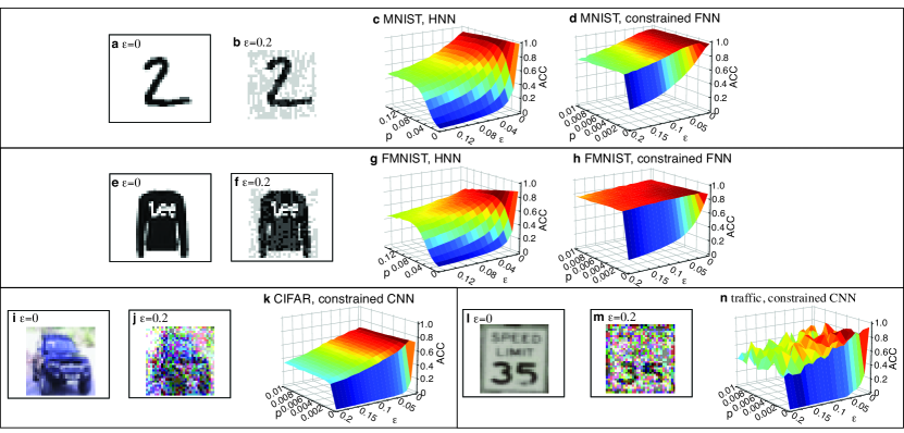
Figure 5: The accuracy (ACC) under adversarial attack. The top panel shows the MNIST image and the image under an adversarial attack with an attack intensity $\epsilon=0.2$. Panels c and d plot the ACC of the hybrid quantum-classical neural network (HNN) and the weight-constrained fully connected neural network (FNN) with a dropout policy. Here, $p$ denotes the dropout probability. The middle panel shows the Fashion MNIST (FMNIST) image and the image under an adversarial attack with an attack intensity $\epsilon=0.2$. Panels g and h plot the ACC of the HNN and the weight-constrained FNN with a dropout policy. The bottom left panel shows the CIFAR image and the image under an adversarial attack with an attack intensity $\epsilon=0.2$. Panel k plots the ACC of the weight-constrained convolutional neural network (CNN) with a dropout policy. The bottom right panel shows the traffic image and the image under an adversarial attack with an attack intensity $\epsilon=0.2$. Panel n plots the ACC of the weight-constrained CNN with a dropout policy.

Adversarial machine learning is an emerging frontier that studies the vulnerability of machine learning systems and develops defense strategies against adversarial attacks. It was demonstrated that quantum machine learning methods for classification tasks are highly vulnerable to adversarial attacks as a result of the concentration of measure phenomenon, which refers to that the distance from a (Haar) randomly sampled point in the Hilbert space to the nearest adversarial example vanishes as $\mathcal{O}(2^{-n})$, where $n$ is the number of qubits [52]. Moreover, it is found that universal adversarial samples can deceive all classifiers with only a perturbation of strength $\mathcal{O}(\mathrm{log}(k)2^{-n})$, where $k$ is the number of independent classifiers [53]. Recently, several approaches have been proposed to improve the resilience of quantum machine learning models, including applying quantum noise [54] and adversarial training [55]. In this work, we propose a new approach to improve adversarial resilience.

In this study, we use the fast gradient sign method (FGSM) to generate adversarial samples (see the Method Section for details) [56]. For the FGSM method, each pixel is modified by $\epsilon\mathrm{sgn}(\nabla_{x}L)$, where $L$ is the loss function and $\epsilon$ represents the strength of the attack. Therefore, a positive value of $\epsilon$ increases the loss function, reducing accuracy. To visualize the adversarial attack, we plot original images and their corresponding adversarially perturbed versions in Figs. 5a, b, e, f, i, j, l, and m.

To enhance the resilience of the quantum machine learning model, we propose randomly dropping $R_{z}$ gates within the quantum circuit of a trained model. In this approach, dropout is immediately added when the model is trained, denoting that attackers have full access only to the loss function of the model after the dropout has been applied. Consequently, adversarial samples are generated using the trained model with the dropout mechanism in place. Figures 5c and 5g plot the ACC of the HNN model under adversarial attack for the MNIST and FMNIST test datasets. Here, $p$ denotes the probability of dropping out. Without the dropout policy ($p=0$), the ACC for both datasets falls rapidly as the attack strength increases $\epsilon$, eventually approaching zero at $\epsilon=0.04$. This result demonstrates the weak resilience of quantum models under adversarial attacks. However, the application of the dropout strategy significantly improves resilience. For example, with $p=0.08$, the ACC for the MNIST dataset drops from 0.968 to 0.567, and for the FMNIST dataset, it drops from 0.774 to 0.555 when $\epsilon$ increases from 0 to 0.1. It is also observed that the ACC for unattacked samples is linearly suppressed by the dropout probability. For example, increasing the probability of dropping out from 0 to 0.08 reduces the ACC by approximately 2% for the MNIST dataset and by 11.2% for the FMNIST dataset. These results highlight that while the dropout method effectively enhances the adversarial resilience of quantum neural networks, it is crucial to carefully select the dropout probability to strike a balance between maintaining ACC for unattacked samples and improving resilience under attack.

The dropout method can also be applied to enhance the adversarial resilience of classical weight-constrained neural networks. Dropping $R_{z}$ gate within a quantum circuit corresponds to changing elements of the weight matrix $W$ shown in Eq. (7). In a weight-constrained neural network, the weight is constructed from the continuous product of the trigonometric function. We can modify the weight by randomly dropping an angle and replacing the trigonometric function related to that angle with a value of one. Figure 5d and Figure 5h illustrate the ACC of the weight-constrained FNN for the MNIST and FMNIST test datasets, respectively. It is found that a small nonzero dropout probability ($p=0.001$) can significantly improve adversarial resilience and make the change of the ACC under attacks tiny. For example, when $p=0.001$ is adopted, the ACC for the FMNIST dataset is only decreased by 0.07 as the attack strength $\epsilon$ increases from 0 to 0.2. Compared to the hybrid quantum-classical model, the weight-constrained FNN requires a smaller value of $p$ to achieve enhanced adversarial resilience. This ensures that the ACC for unattacked samples remains almost unaffected when such a small $p$ is adopted. Furthermore, Figs. 5k and 5n depict the ACC of the weight-constrained CNN, which is trained on the CIFAR and traffic datasets. Similarly, the dropout method with $p=0.001$ substantially improves adversarial resilience. The oscillatory behavior observed in Fig. 5n can be attributed to the small sample size of the traffic test dataset (50 samples), which lacks sufficient statistical robustness.

We note that the success of our approach on the traffic dataset is critical to ensuring the safety of self-driving vehicles [57, 58]. In these vehicles, CNN-based regression models are widely used for object recognition. However, CNNs have been shown to be highly susceptible to adversarial samples [59]. To address this issue, numerous studies have focused on improving the adversarial resilience of CNNs [60, 61]. Our work introduces a novel method to improve CNN resilience, thus improving the safety and reliability of self-driving vehicles.

Overview of the benefits of the weight-constrained neural network

In machine learning, regularization and early stopping are commonly employed to mitigate overfitting. Our developed weight-constrained neural network introduces an alternative approach to addressing this issue. By limiting learnability, the weight-constrained neural network effectively filters out noise in training data while capturing essential signals, thereby suppressing overfitting.

Beyond suppressing overfitting, the weight-constrained method significantly reduces memory and storage requirements. In standard neural networks, all weights must be stored in memory, causing memory usage to scale linearly with the number of weights. In addition, large AI models require substantial storage to save trained parameters. The weight-constrained method can reduce these costs. For example, memory usage can be optimized by temporarily constructing and releasing the weight matrix after use. In addition, the memory cost for storing gradients of weights can also be reduced by adopting the weight-constrained method. This reduction is particularly critical for large-scale AI models. For example, a model with one billion parameters requires 8 GB of memory for weights and corresponding gradients with float-32 precision. By applying the weight-constrained method, the number of variables can be reduced by a factor of 100, reducing the memory requirement to just 81 MB.

To effectively apply QML to industry challenges, ensuring the security of QML models is paramount. Although standard classical techniques, such as adversarial training [55], can enhance the resilience of QML models, our work introduces an alternative approach that takes advantage of the intrinsic properties of quantum circuits. Additionally, our developed dropout method, based on the weight-constrained method, enriches techniques to improve the robustness of classical machine learning models.

Conclusion

In this work, we explore the underlying mathematical principles of quantum neural networks with angle and amplitude encodings. Drawing inspiration from these principles, we develop a classical weight-constrained neural network that helps mitigate overfitting and reduces memory requirements. Additionally, we develop a dropout approach to enhance the adversarial resilience of both quantum neural networks and classical weight-constrained neural networks. These findings are crucial for the application of machine learning in industrial settings.

Our study did not assess the performance of the weight-constrained transformer models. Recently, a quantum version of the transformer model was proposed in Ref. 62, which uses a quantum circuit with amplitude encoding to compute attention coefficients. This approach demonstrated a quantum advantage, achieving a higher accuracy in simulations using the MedMNIST dataset. Building on these results, it would be interesting to investigate the performance of the weight-constrained method within transformer networks. Our work employs a combinatorial method and trigonometric functions to construct weights. It is also valuable to explore alternative methods to construct weights (see Supplementary Note 2).

Ref. 63 observed that any algorithm that performs well in one problem is likely to perform poorly in another. Our proposed weight-constrained method effectively reduces memory usage; however, it increases computational time due to the dynamic memory allocation required for constructing weights. Striking a balance between memory consumption and computational efficiency requires determining the optimal number of weights to be constructed using this method. However, we note that the need for dynamically constructing weight matrices is not required on quantum computers; therefore, quantum machine learning has advantages in both reducing memory consumption and improving computational efficiency.

Method

Datasets

In our study, we adopted four different datasets: MNIST, Fashion MNIST, CIFAR, and a real-world traffic sign dataset derived from the LISA Traffic Sign Dataset [64] and the Mapillary Traffic Sign Dataset [65]. For each dataset, only five classes were selected as samples. For the MNIST, FMNIST, and CIFAR datasets, we use 30,000 samples for training and 5,000 samples for testing. The traffic sign dataset has fewer samples, so we use 200 samples for training and 50 samples for testing.

Adversarial samples

In classical adversarial machine learning, adversarial samples can be generated using different approaches, such as the fast gradient sign method [56], the basic iterative method [66], and the projected gradient descent method [67]. In this work, we adopted the fast gradient sign method to generate adversarial samples ${\bf x}^{*}$, which is frequently applied in the literature [68]. For the FGSM method, each pixel is modified as

$${\bf x}^{*}={\bf x}+\epsilon\cdot\mathrm{sgn}(\nabla_{x}L),$$ (14)

where $L$ is the loss function of the trained model, $\epsilon$ is the attacking strength, and $\nabla_{x}$ denotes the gradient of the loss with respect to sample ${\bf x}$. In practice, we restrict that $0\leq{\bf x}^{*}\leq 1$. Equation (14) shows that each pixel is modified to enlarge the loss function, thus reducing the accuracy.

Data Availability

The data that support the findings of this study are available from the corresponding authors upon reasonable request.

Code Availability

The code is available at https://github.com/sli43/hybrid-quantum-classical-CNN.

Author contributions

S.L. implemented codes and performed simulations. All authors contributed to the discussion and writing of the manuscript.

Competing interests

The authors declare no competing interests.

Additional Information

Supplementary Information accompanies this paper at Insert_link.
Correspondence and requests for materials should be addressed to Shaozhi Li.

References

- [1] Soori, M., Arezoo, B. & Dastres, R. Artificial intelligence, machine learning and deep learning in advanced robotics, a review. \JournalTitleCognitive Robotics 3, 54–70, DOI: https://doi.org/10.1016/j.cogr.2023.04.001 (2023).
- [2] Gozalo-Brizuela, R. & Garrido-Merchan, E. C. ChatGPT is not all you need. A State of the Art Review of large Generative AI models. \JournalTitlearXiv: 2301.04655 DOI: https://arxiv.org/abs/2301.04655 (2023).
- [3] Thirunavukarasu, A. J. et al. Large Language models in medicine. \JournalTitleNature Medicine 29, 1930–1940, DOI: https://doi.org/10.1038/s41591-023-02448-8 (2023).
- [4] Min, B. et al. Recent Advances in Natural Language Processing via Large Pre-trained Language Models: A Survey. \JournalTitleACM Comput. Surv. 56, DOI: 10.1145/3605943 (2023).
- [5] Liu, Y. et al. Summary of ChatGPT-Related research and perspective towards the future of large language models. \JournalTitleMeta-Radiology 1, 100017, DOI: https://doi.org/10.1016/j.metrad.2023.100017 (2023).
- [6] Qiu, J. et al. Large AI Models in Health Informatics: Applications, Challenges, and the Future. \JournalTitleIEEE Journal of Biomedical and Health Informatics 27, 6074–6087, DOI: 10.1109/JBHI.2023.3316750 (2023).
- [7] Devlin, J., Chang, M.-W., Lee, K. & Toutanova, K. BERT: Pre-training of Deep Bidirectional Transformers for Language Understanding. \JournalTitlearXiv: 1810.04805 DOI: https://arxiv.org/abs/1810.04805 (2019).
- [8] Jumper, J. et al. Highly accurate protein structure prediction with AlphaFold. \JournalTitleNature 596, 583–589, DOI: 10.1038/s41586-021-03819-2 (2021).
- [9] Varadi, M. et al. AlphaFold Protein Structure Database in 2024: providing structure coverage for over 214 million protein sequences. \JournalTitleNucleic Acids Research 52, D368–D374, DOI: 10.1093/nar/gkac1117 (2024).
- [10] Allen-Zhu, Z., Li, Y. & Liang, Y. Learning and Generalization in Overparameterized Neural Networks, Going Beyond Two Layers. \JournalTitlearXiv: 1811.04918 DOI: https://arxiv.org/abs/1811.04918 (2020).
- [11] Erhan, D., Manzagol, P.-A., Bengio, Y., Bengio, S. & Vincent, P. The Difficulty of Training Deep Architectures and the Effect of Unsupervised Pre-Training. In van Dyk, D. & Welling, M. (eds.) Proceedings of the Twelfth International Conference on Artificial Intelligence and Statistics, vol. 5 of Proceedings of Machine Learning Research, 153–160, DOI: https://proceedings.mlr.press/v5/erhan09a.html (PMLR, Hilton Clearwater Beach Resort, Clearwater Beach, Florida USA, 2009).
- [12] Bachlechner, T., Majumder, B. P., Mao, H., Cottrell, G. & McAuley, J. ReZero is all you need: fast convergence at large depth. In de Campos, C. & Maathuis, M. H. (eds.) Proceedings of the Thirty-Seventh Conference on Uncertainty in Artificial Intelligence, vol. 161 of Proceedings of Machine Learning Research, 1352–1361, DOI: https://proceedings.mlr.press/v161/bachlechner21a.html (PMLR, 2021).
- [13] Arute, F. et al. Quantum supremacy using a programmable superconducting processor. \JournalTitleNature 574, 505–510, DOI: 10.1038/s41586-019-1666-5 (2019).
- [14] Schuld, M. & Killoran, N. Is Quantum Advantage the Right Goal for Quantum Machine Learning? \JournalTitlePRX Quantum 3, 030101, DOI: 10.1103/PRXQuantum.3.030101 (2022).
- [15] Du, Y., Hsieh, M.-H., Liu, T. & Tao, D. Expressive power of parametrized quantum circuits. \JournalTitlePhys. Rev. Res. 2, 033125, DOI: 10.1103/PhysRevResearch.2.033125 (2020).
- [16] Alcazar, J., Vakili, M. G., Kalayci, C. B. & Perdomo-Ortiz, A. GEO: Enhancing Combinatorial Optimization with Classical and Quantum Generative Models. \JournalTitlearXiv: 2101.06250 DOI: https://arxiv.org/abs/2101.06250 (2022).
- [17] Cerezo, M., Verdon, G., Huang, H.-Y., Cincio, L. & Coles, P. J. Challenges and opportunities in quantum machine learning. \JournalTitleNature Computational Science 2, 567–576, DOI: https://doi.org/10.1038/s43588-022-00311-3 (2022).
- [18] Liu, Y., Arunachalam, S. & Temme, K. A rigorous and robust quantum speed-up in supervised machine learning. \JournalTitleNature Physics 17, 1013–1017, DOI: https://doi.org/10.1038/s41567-021-01287-z (2021).
- [19] Paparo, G. D., Dunjko, V., Makmal, A., Martin-Delgado, M. A. & Briegel, H. J. Quantum Speedup for Active Learning Agents. \JournalTitlePhys. Rev. X 4, 031002, DOI: 10.1103/PhysRevX.4.031002 (2014).
- [20] Wiebe, N., Braun, D. & Lloyd, S. Quantum Algorithm for Data Fitting. \JournalTitlePhys. Rev. Lett. 109, 050505, DOI: 10.1103/PhysRevLett.109.050505 (2012).
- [21] Huang, H.-Y. et al. Power of data in quantum machine learning. \JournalTitleNature Communications 12, 2631, DOI: 10.1038/s41467-021-22539-9 (2021).
- [22] Huang, H.-Y. et al. Quantum advantage in learning from experiments. \JournalTitleScience 376, 1182–1186, DOI: 10.1126/science.abn7293 (2022). https://www.science.org/doi/pdf/10.1126/science.abn7293.
- [23] Salek, M. S., Li, S. & Chowdhury, M. A hybrid quantum-classical ai-based detection strategy for generative adversarial network-based deepfake attacks on an autonomous vehicle traffic sign classification system. \JournalTitlearXiv: 2409.17311 DOI: https://arxiv.org/abs/2409.17311 (2024).
- [24] Rebentrost, P., Mohseni, M. & Lloyd, S. Quantum support vector machine for big data classification. \JournalTitlePhys. Rev. Lett. 113, 130503, DOI: 10.1103/PhysRevLett.113.130503 (2014).
- [25] Biamonte, J. et al. Quantum machine learning. \JournalTitleNature 549, 195–202, DOI: https://doi.org/10.1038/nature23474 (2017).
- [26] Ciliberto, C. et al. Quantum machine learning: a classical perspective. \JournalTitleProceedings of the Royal Society A: Mathematical, Physical and Engineering Sciences 474, 20170551, DOI: https://doi.org/10.1098/rspa.2017.0551 (2018).
- [27] Beer, K. et al. Training deep quantum neural networks. \JournalTitleNature Communications 11, 808, DOI: https://doi.org/10.1038/s41467-020-14454-2 (2020).
- [28] Schuld, M. Supervised quantum machine learning models are kernel methods. \JournalTitlearXiv: 2101.11020 DOI: https://doi.org/10.48550/arXiv.2101.11020 (2021).
- [29] Blank, C., Park, D. K., Rhee, J.-K. K. & Petruccione, F. Quantum classifier with tailored quantum kernel. \JournalTitlenpj Quantum Information 6, 41, DOI: https://doi.org/10.1038/s41534-020-0272-6 (2020).
- [30] Zoufal, C., Lucchi, A. & Woerner, S. Quantum generative adversarial networks for learning and loading random distributions. \JournalTitlenpj Quantum Information 5, 103, DOI: https://doi.org/10.1038/s41534-019-0223-2 (2019).
- [31] Havlíček, V. et al. Supervised learning with quantum-enhanced feature spaces. \JournalTitleNature 567, 209–212, DOI: https://doi.org/10.1038/s41586-019-0980-2 (2019).
- [32] Huang, K. et al. Quantum generative adversarial networks with multiple superconducting qubits. \JournalTitlenpj Quantum Information 7, 165, DOI: https://doi.org/10.1038/s41534-021-00503-1 (2021).
- [33] Tancara, D., Dinani, H. T., Norambuena, A., Fanchini, F. F. & Coto, R. Kernel-based quantum regressor models learning non-Markovianity. \JournalTitlePhys. Rev. A 107, 022402, DOI: 10.1103/PhysRevA.107.022402 (2023).
- [34] Slattery, L. et al. Numerical evidence against advantage with quantum fidelity kernels on classical data. \JournalTitlePhys. Rev. A 107, 062417, DOI: https://doi-org.libproxy.clemson.edu/10.1103/PhysRevA.107.062417 (2023).
- [35] Benedetti, M., Realpe-Gómez, J. & Perdomo-Ortiz, A. Quantum-assisted helmholtz machines: A quantum–classical deep learning framework for industrial datasets in near-term devices. \JournalTitleQuantum Science and Technology 3, 034007, DOI: 10.1088/2058-9565/aabd98 (2018).
- [36] Perdomo-Ortiz, A., Benedetti, M., Realpe-Gómez, J. & Biswas, R. Opportunities and challenges for quantum-assisted machine learning in near-term quantum computers. \JournalTitleQuantum Science and Technology 3, 030502, DOI: 10.1088/2058-9565/aab859 (2018).
- [37] Rudolph, M. S. et al. Generation of high-resolution handwritten digits with an ion-trap quantum computer. \JournalTitlePhys. Rev. X 12, 031010, DOI: 10.1103/PhysRevX.12.031010 (2022).
- [38] Krunic, Z., Flother, F., Seegan, G., Earnest-Noble, N. & Omar, S. Quantum kernels for real-world predictions based on electronic health records. \JournalTitleIEEE Transactions on Quantum Engineering 3, 1–11, DOI: 10.1109/tqe.2022.3176806 (2022).
- [39] Moradi, S. et al. Error mitigation for quantum kernel based machine learning methods on ionq and ibm quantum computers. \JournalTitlearXiv: 2206.01573 DOI: https://arxiv.org/abs/2206.01573 (2022).
- [40] Terhal, B. M. Quantum error correction for quantum memories. \JournalTitleRev. Mod. Phys. 87, 307–346, DOI: 10.1103/RevModPhys.87.307 (2015).
- [41] Knill, E., Laflamme, R. & Viola, L. Theory of quantum error correction for general noise. \JournalTitlePhys. Rev. Lett. 84, 2525–2528, DOI: 10.1103/PhysRevLett.84.2525 (2000).
- [42] Tang, E. A quantum-inspired classical algorithm for recommendation systems. In Proceedings of the 51st Annual ACM SIGACT Symposium on Theory of Computing, STOC 2019, 217–228, DOI: 10.1145/3313276.3316310 (Association for Computing Machinery, New York, NY, USA, 2019).
- [43] Felser, T. et al. Quantum-inspired machine learning on high-energy physics data. \JournalTitlenpj Quantum Information 7, 111, DOI: https://doi.org/10.1038/s41534-021-00443-w (2021).
- [44] Duong, T. Q. et al. Quantum-inspired machine learning for 6g: Fundamentals, security, resource allocations, challenges, and future research directions. \JournalTitleIEEE Open Journal of Vehicular Technology 3, 375–387, DOI: 10.1109/OJVT.2022.3202876 (2022).
- [45] Ding, C., Bao, T.-Y. & Huang, H.-L. Quantum-inspired support vector machine. \JournalTitleIEEE Transactions on Neural Networks and Learning Systems 33, 7210–7222, DOI: 10.1109/TNNLS.2021.3084467 (2022).
- [46] Wall, M. L. & D’Aguanno, G. Tree-tensor-network classifiers for machine learning: From quantum inspired to quantum assisted. \JournalTitlePhys. Rev. A 104, 042408, DOI: 10.1103/PhysRevA.104.042408 (2021).
- [47] Li, S., Salek, M. S., Wang, Y. & Chowdhury, M. Quantum-inspired activation functions and quantum Chebyshev-polynomial network, DOI: https://arxiv.org/abs/2404.05901 (2024).
- [48] Tiwari, P. & Melucci, M. Towards a Quantum-Inspired Binary Classifier. \JournalTitleIEEE Access 7, 42354–42372, DOI: 10.1109/ACCESS.2019.2904624 (2019).
- [49] Cong, I., Choi, S. & Lukin, M. D. Quantum convolutional neural networks. \JournalTitleNature Physics 15, 1273–1278, DOI: 10.1038/s41567-019-0648-8 (2019).
- [50] Sim, S., Johnson, P. D. & Aspuru-Guzik, A. Expressibility and Entangling Capability of Parameterized Quantum Circuits for Hybrid Quantum-Classical Algorithms. \JournalTitleAdvanced Quantum Technologies 2, 1900070, DOI: https://onlinelibrary.wiley.com/doi/abs/10.1002/qute.201900070 (2019).
- [51] McClean, J. R., Boixo, S., Smelyanskiy, V. N., Babbush, R. & Neven, H. Barren plateaus in quantum neural network training landscapes. \JournalTitleNature Communications 9, 4812, DOI: 10.1038/s41467-018-07090-4 (2018).
- [52] Liu, N. & Wittek, P. Vulnerability of quantum classification to adversarial perturbations. \JournalTitlePhys. Rev. A 101, 062331, DOI: 10.1103/PhysRevA.101.062331 (2020).
- [53] Gong, W. & Deng, D.-L. Universal adversarial examples and perturbations for quantum classifiers. \JournalTitleNational Science Review 9, nwab130, DOI: 10.1093/nsr/nwab130 (2022).
- [54] Du, Y., Hsieh, M.-H., Liu, T., Tao, D. & Liu, N. Quantum noise protects quantum classifiers against adversaries. \JournalTitlePhys. Rev. Res. 3, 023153, DOI: 10.1103/PhysRevResearch.3.023153 (2021).
- [55] Lu, S., Duan, L.-M. & Deng, D.-L. Quantum adversarial machine learning. \JournalTitlePhys. Rev. Res. 2, 033212, DOI: 10.1103/PhysRevResearch.2.033212 (2020).
- [56] Goodfellow, I. J., Shlens, J. & Szegedy, C. Explaining and Harnessing Adversarial Examples. \JournalTitlearXiv: 1412.6572 DOI: https://arxiv.org/abs/1412.6572 (2015).
- [57] Chowdhury, A., Karmakar, G., Kamruzzaman, J., Jolfaei, A. & Das, R. Attacks on self-driving cars and their countermeasures: A survey. \JournalTitleIEEE Access 8, 207308–207342, DOI: 10.1109/ACCESS.2020.3037705 (2020).
- [58] Deng, Y. et al. An analysis of adversarial attacks and defenses on autonomous driving models. In 2020 IEEE International Conference on Pervasive Computing and Communications (PerCom), 1–10, DOI: 10.1109/PerCom45495.2020.9127389 (2020).
- [59] Goodfellow, I. J., Shlens, J. & Szegedy, C. Explaining and harnessing adversarial examples. \JournalTitlearXiv: 1412.6572 (2015).
- [60] Papernot, N., McDaniel, P., Wu, X., Jha, S. & Swami, A. Distillation as a defense to adversarial perturbations against deep neural networks. In 2016 IEEE Symposium on Security and Privacy (SP), 582–597, DOI: 10.1109/SP.2016.41 (2016).
- [61] Wong, E. & Kolter, Z. Provable defenses against adversarial examples via the convex outer adversarial polytope. In Dy, J. & Krause, A. (eds.) Proceedings of the 35th International Conference on Machine Learning, vol. 80 of Proceedings of Machine Learning Research, 5286–5295, DOI: https://proceedings.mlr.press/v80/wong18a.html (PMLR, 2018).
- [62] Cherrat, E. A. et al. Quantum vision transformers. \JournalTitleQuantum 8, 1265, DOI: 10.22331/q-2024-02-22-1265 (2024).
- [63] Wolpert, D. H. The Lack of A Priori Distinctions Between Learning Algorithms. \JournalTitleNeural Computation 8, 1341–1390, DOI: 10.1162/neco.1996.8.7.1341 (1996).
- [64] Mogelmose, A., Trivedi, M. M. & Moeslund, T. B. Vision-Based Traffic Sign Detection and Analysis for Intelligent Driver Assistance Systems: Perspectives and Survey. \JournalTitleIEEE Transactions on Intelligent Transportation Systems 13, 1484–1497, DOI: 10.1109/TITS.2012.2209421 (2012).
- [65] Ertler, C. et al. The Mapillary Traffic Sign Dataset for Detection and Classification on a Global Scale. \JournalTitlearXiv: 1909.04422 DOI: https://arxiv.org/abs/1909.04422 (2020).
- [66] Kurakin, A., Goodfellow, I. & Bengio, S. Adversarial Machine Learning at Scale. \JournalTitlearXiv: 1611.01236 DOI: https://arxiv.org/abs/1611.01236 (2017).
- [67] Madry, A., Makelov, A., Schmidt, L., Tsipras, D. & Vladu, A. Towards Deep Learning Models Resistant to Adversarial Attacks. \JournalTitlearXiv: 1706.06083 DOI: https://arxiv.org/abs/1706.06083 (2019).
- [68] Li, C., Wang, H., Zhang, J., Yao, W. & Jiang, T. An approximated gradient sign method using differential evolution for black-box adversarial attack. \JournalTitleIEEE Transactions on Evolutionary Computation 26, 976–990, DOI: 10.1109/TEVC.2022.3151373 (2022).
Acknowledgement
This work is supported by the National Center for Transportation Cybersecurity and Resiliency (TraCR) (a U.S. Department of Transportation National University Transportation Center) headquartered at Clemson University, Clemson, South Carolina, USA. Y.W. acknowledges support from the U.S. Department of Energy, Office of Science, Basic Energy Sciences, under Early Career Award No. DE-SC0024524. Any opinions, findings, conclusions, and recommendations expressed in this material are those of the author(s) and do not necessarily reflect the views of TraCR. The U.S. Government assumes no liability for the contents or use thereof. We acknowledge the computational support from Palmetto2, a high-performance computing cluster at Clemson University.