Estimation of the frequency-shift between two photons by time-sampling measurements

Abstract

We present a sensing scheme for estimating the frequency difference of two non-entangled photons. The technique consists of time-resolving sampling measurements at the output of a beam splitter. With this protocol, the frequency shift between two photons can be estimated with the ultimate precision achievable in nature, overcoming the limits in precision and the range of detection of frequency-resolving detectors employed in standard direct measurements of the frequencies. The sensitivity can be increased by increasing the coherence time of the photons. We show that, already with $\sim 1000$ sampling measurements, the Cramér-Rao bound is saturated independently of the value of the difference in frequency.

I Introduction

When two photons impinge on a balanced beam splitter from its two input ports, a well-known two-photon interference effect occurs Hong et al. (1987); Shih and Alley (1988). In particular, if the photons are completely identical in all their degrees of freedom, they will always reach one of the two output ports simultaneously (they will always bunch). This phenomenon has been widely applied in quantum information, e.g., quantum computing Kok et al. (2007); Barz et al. (2012), quantum key distribution Tang et al. (2014); Guan et al. (2015), quantum repeater Sangouard et al. (2011); Hofmann et al. (2012), and quantum coherence tomography Teich et al. (2012).

When the two photons are not completely identical, the probability of them reaching two different output ports (the probability of having a coincidence event) is not zero and depends on the overlap between the two single-photon states. It is thus possible to retrieve the value of a physical property encoded in such overlap by measuring the coincidence rate. Indeed, this interference effect has several applications in quantum metrology, and it has been used for evaluating time delays between the photons Lyons et al. (2018), frequency Gerrits et al. (2015); Jin et al. (2015); Gianani et al. (2018); Fabre and Felicetti (2021), and polarization Harnchaiwat et al. (2020); Sgobba et al. (2023).

More recently, it was shown that it is possible to maximize the sensitivity in estimating relative photonic parameters, such as time delay or transverse displacement, by resolving their frequencies or their transverse momenta Triggiani et al. (2023); Triggiani and Tamma (2024). The ultimate precision is achieved under the assumption of unit detector efficiency and perfect overlap of all the photonic degrees of freedom but the one to measure.

However, achieving the ultimate quantum precision in the measurement of the photonic frequencies remains an experimental challenge. Indeed, standard techniques that rely on the direct measurement of such frequencies are limited by the precision of the employed frequency-resolved detectors.

In this work, we present a two-photon interferometry technique for measuring the frequency shift between two photons with ultimate quantum precision. The sensing scheme is based on sampling time-resolving measurements of these photons after they impinge on a beam splitter. The precision that it is possible to reach with such a scheme is independent of the values of the relative photonic frequency we wish to estimate. This sensing protocol can have applications in vibrometry Rehain et al. (2021), characterization of biological material, or optical coherence tomography Kolenderska et al. (2020).

In this article, we describe the experimental setup in detail and evaluate its efficiency in a quantum metrology framework. With this setup, the frequency shift between two photons can be estimated with the ultimate precision, under the assumption of unit detector efficiency and perfect overlap of all the degrees of freedom of the two photons but the frequency. Also, we discuss the regime in which the ultimate precision is not achieved. We provide a comparison between this setup and a non-resolving protocol, proving that time-resolution measurements improve the estimation, especially in a high frequency-shift regime. Already with $\sim 1000$ sampling measurements, the Cramér-Rao bound is saturated, independently of the value of the frequency shift.

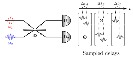
Figure 1: Sensing scheme. Two photons, with central frequencies $\omega_{1}$ and $\omega_{2}$, described in the temporal domain in (1) enter in the input channel of a 50:50 beam splitter (BS). Then, their temporal delay is resolved with two detectors $D_{1}$ and $D_{2}$. Here, for example, three repetitions of the experiment are illustated, in which the temporal delays $\Delta t_{A}$, $\Delta t_{B}$, $\Delta t_{C}$, are recorded. These delays, correspond to a bunching event, a coincidence event and a bunching event, respectively.

II Experimental setup

In this section we describe the experimental setup in FIG.1. A pair of photons impinges on a balanced beam splitter, respectively, through its two input ports. The photons are prepared with a temporal amplitude $\psi_{s}\left(t\right)=\left|\psi\left(t\right)\right|\mathrm{e}^{-i\omega_{s}t}$ with $s=1,2$. The parameter $\omega_{s}$ is the centre of the s-th photon frequency distribution. The bosonic operators $\hat{a}^{\dagger}_{1}(t_{1})$ and $\hat{b}^{\dagger}_{2}(t_{2})$ are function of the input channel $s$ at time $t_{s}$ ($s=1,2$). They are defined as the Fourier transforms of the bosonic operators in the frequency domain. Their commutation relation is $\left[\hat{a}_{s}(t_{1}),\hat{b}^{\dagger}_{s^{\prime},t_{2}}\right]=\sqrt{\nu}\delta_{ss^{\prime}}\delta\left(t_{1}-t_{2}\right)$, where $\delta_{ss^{\prime}}$ and $\delta\left(t_{1}-t_{2}\right)$ are respectively the Kroenecker delta in function of the input channels, and the Dirac delta in the time domain. The parameter $\nu\in\left[0,1\right]$ represents the degree of indistinguishability of the two photons in any other degree of freedom that is not the time. The two-photon input state thus reads

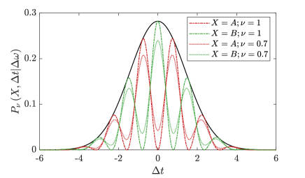
Figure 2: Plot of the probability distribution in eq. 3. The temporal distribution $\left|\psi\left(t\right)\right|^{2}$ is considered Gaussian with unitary variance. This yields a Gaussian envelope $C\left(\Delta t\right)$, represented by the black line. The choice of the variance fixed a natural scale for $\Delta t$ and for $\Delta\omega=4/\tau$

.

$$\left|\bm{\psi}\right\rangle=\int_{\mathbb{R}^{2}}dt_{1}dt_{2}\psi_{1}\left(t_{1}\right)\psi_{2}\left(t_{2}\right)\hat{a}^{\dagger}_{1}(t_{1})\hat{b}^{\dagger}_{2}(t_{2})\left|0\right\rangle,$$ (1)

where $\left|0\right\rangle=\left|0\right\rangle_{1}\otimes\left|0\right\rangle_{2}$ is the vacuum state.

Two detectors are connected to the two output channels of the beam splitter. They are sensitive to the time of arrival of the two photons. This experimental setup does not directly measure the frequency of the photons; instead, the sensing protocol relies on time-sampling measurementsLegero et al. (2003). The measure of the time delay between the two photons can be done with a precision of the order of the psKorzh et al. (2020); Nolet et al. (2018); Esmaeil Zadeh et al. (2017); Wu et al. (2017). The only requirement for the precision in time $\delta t$ is to be high enough to erase the indistinguishability in time of the two photons, e.g. for Gaussian distribution in time with variance $\tau$, the requirement for the estimation of $\Delta\omega=\omega_{2}-\omega_{1}$ is

$$\delta t\ll\frac{1}{|\Delta\omega|}\qquad\mathrm{and}\qquad\delta t\ll\tau.$$ (2)

For example, this means that already by employing detectors with a time resolution $\delta t\approx 10$ ps, it is possible to estimate a range of values of $\Delta\omega$ up to the range $10$ GHz, or up to the range $100$ GHz without changing the experimental setup if one can employ detectors with resolution $\delta t$ of the order of 1 ps. Indeed, state-of-the-art time-resolving detectors can already achieve a resolution of few ps Wu et al. (2017); Nolet et al. (2018); Esmaeil Zadeh et al. (2017); Korzh et al. (2020). As long as this bound in $\Delta\omega$ is respected, the values of $\omega_{1}$ and $\omega_{2}$ can be in any frequency range, overcoming the range limitations of standard spectrometers Davis et al. (2017); Hiemstra et al. (2020). Furthermore, the second condition in Eq.(2) is easily satisfied with the state-of-the-art single-photon sources Zhao et al. (2014); Wang et al. (2024).

In this setup, the two photons can arrive on the same output channel (bunching, labeled with the letter A) or they can arrive on two different output channels (coincidence, labeled with the letter B). In addition, the two photons impinge on the detectors with a certain time delay $\Delta t$. The probability of having $X=A,B$ and a specific $\Delta t$ is

$$P_{\nu}\left(X,\Delta t|\Delta\omega\right)=\frac{C\left(\Delta t\right)}{2}\Bigg{(}1+\nu\alpha\left(X\right)\cos\left(\Delta\omega\Delta t\right)\Bigg{)},$$ (3)

where $\alpha\left(A\right)=1$, $\alpha\left(B\right)=-1$, and $C\left(\Delta t\right)$ is the beats envelope, whose shape can be evaluated by using $\psi\left(t\right)$. We plot this probability in function of $\Delta t$ in FIG. 2. In particular, for two Gaussian distributions in time with variance $\tau$, $C\left(\Delta t\right)$ assumes the form

$$C\left(\Delta t\right)=\frac{1}{\sqrt{4\pi\tau^{2}}}\mathrm{exp}\left[-\frac{\Delta t^{2}}{4\tau^{2}}\right].$$ (4)

By introducing the efficiency of the detectors $\gamma\in\left[0,1\right]$ (assumed to be equal for both detectors), it is possible to define the probability of measuring $0,1,2$ photons in output with probabilities that are, respectively

$$\begin{cases}&P_{0}=\left(1-\gamma\right)^{2}\\ &P_{1}=2\gamma\left(1-\gamma\right)\\ &P_{2}\left(X,\Delta t|\Delta\omega\right)=\gamma^{2}P_{\nu}\left(X,\Delta t|\Delta\omega\right),\qquad X=A,B\end{cases}.$$ (5)

Only the probability $P_{2}\left(X,\Delta t|\Delta\omega\right)$ is function of the parameter $\Delta\omega$. This probability is proportional to the one previously found in Eq (3) by a factor $\gamma^{2}$.

III Ultimate quantum sensitivity

An unbiased estimator of the frequency shift $\widetilde{\Delta\omega}$ is affected by an error described by the variance $\mathrm{Var}[\widetilde{\Delta\omega}]$. This variance will always be bounded below by the Cramér-Rao bound, which represents the maximum precision achievable by the sensing protocol and it is a function of the Fisher information $F_{\nu}\left(\Delta\omega\right)$ and the number of iterations of the experiment $N$Cramér (1999); Rohatgi and Saleh (2015). This bound is always saturated in the asymptotic limit of large $N$. Ultimately, the Cramér-Rao bound is bounded from below by the quantum Cramér-Rao bound, which is the maximum precision achievable by any scheme, independently of the chosen type of measurement, and it depends on the quantum Fisher information $H\left(\Delta\omega\right)$ and $N$Helstrom (1969); Holevo (2011). Therefore, the following inequalities hold

$$\mathrm{Var}\left[\widetilde{\Delta\omega}\right]\geq\frac{1}{NF_{\nu}\left(\Delta\omega\right)}\geq\frac{1}{NH\left(\Delta\omega\right)}.$$ (6)

In particular, by using the probabilities in Eq. (5), the Fisher information assumes the form

$$F_{\nu=1}\left(\Delta\omega\right)=\gamma^{2}H\left(\Delta\omega\right)=2\gamma^{2}\tau^{2},$$ (7)

proving that under the condition of unit detection efficiency, this sensing protocol reaches the ultimate precision for $\nu=1$. This happens because for $\nu=1$ the detectors cannot distinguish at all the two input photons, enhancing the two-photon interference. Interestingly, the overlap of the density distributions of the two photons in the frequency domain does not affect the asymptotic sensitivity of the sensing scheme. Also, the dependence of the Fisher information only on the coherence time is an advantage with respect to the standard direct measurements, since these operate only in a specific range of frequencies and their precision is limited by their finite resolution. Remarkably, our technique allows us to obtain a precision of already the order of $0.1$ MHz (which corresponds, for example, in the visible range to a precision of the order of 20 am for wavelengths of the order of 800 nm) for $\tau^{2}N=10^{7}\mathrm{ns}^{2}$, achievable for example with a coherence time $\tau=100$ ns McKeever et al. (2004); Wilk et al. (2007); Keller et al. (2004) and just a number of sampling measurements $N\sim 10^{3}$, or increasing accordingly the number of measurements if photons of smaller coherence times are employed. Therefore, this technique outperforms the precision of most standard spectrometers in the state-of-the-art Davis et al. (2017); Hiemstra et al. (2020).

IV Contribution to the sampled time delay

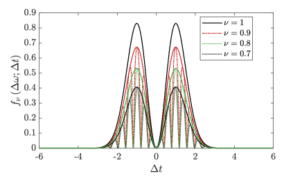
Figure 3: Contributions $f_{\nu}\left(\Delta\omega;\Delta t\right)$ in the Fisher information as a function of the sampled time delay $\Delta t$ for different values of the parameter $\nu$. The plot is for a Gaussian distribution in time of the two photons $\left|\psi\left(t\right)\right|^{2}$ with variance $\tau$. The variance fixes a natural scale for $\Delta t$ and for $\Delta\omega=4/\tau_{\Delta t}$. The solid lines represent the envelope of $f_{\nu}\left(\Delta\omega;\Delta t\right)$ and show the contribution of the Fisher information that is significant or negligible.

Our sensing protocol remains effective even by using as input two photons that are partially distinguishable in all the degrees of freedom but the time. This is the case in which $\nu<1$ and the Fisher information reads

$$F_{\nu}\left(\Delta\omega\right) =\gamma^{2}\int dtf_{\nu}\left(\Delta\omega;t\right)=$$ (8)

$$=\gamma^{2}\int_{\mathbb{R}}dtC\left(t\right)t^{2}\beta_{\nu}\left(\Delta\omega t\right),$$ (9)

where $f_{\nu}\left(\Delta\omega;\Delta t\right)$ is the contribution of each $\Delta t$ to the Fisher information. Also, the function $\beta_{\nu}\left(\xi\right)$ is defined as follows (for more details see Appendix C):

$$\beta_{\nu}\left(\xi\right)=\frac{\nu^{2}\sin^{2}\left(\xi\right)}{1-\nu^{2}\cos^{2}\left(\xi\right)}.$$ (10)

For Gaussian distributions, the Fisher information  (9) specialises into

$$F^{G}_{\nu}\left(\Delta\omega\right)=\frac{2F_{\nu=1}\left(\Delta\omega\right)}{\sqrt{\pi}}\int_{\mathbb{R}}\mathrm{d}\kappa\,\mathrm{e}^{-\kappa^{2}}\kappa^{2}\beta_{\nu}\left(2\tau\Delta\omega\kappa\right).$$ (11)

We plot the contribution of the Fisher information $f_{\nu}\left(\Delta\omega;\Delta t\right)$ in FIG. 3, where we show the amount of information obtained for each sampled time delay. In particular, we show that $f_{\nu}\left(\Delta\omega;\Delta t\right)$ is concentrated within its envelope, that is, $\nu^{2}C\left(\Delta t\right)\Delta t^{2}/2\tau^{2}$. The envelope is independent of $\Delta\omega$, which means that the metrological scheme does not need to be calibrated according to the parameter to estimate $\Delta\omega$.

We show the efficiency of the sensing scheme in FIG 4 which exploits the simulated variance of the likelihood estimator Rohatgi and Saleh (2015) normalized to the Cramér-Rao bound. It is evident that for a number of sampling measurements $N\sim 1000$ the Cramér-Rao bound is saturated. In the insets, we show the expected value $E\left[\widetilde{\Delta\omega}\right]$ of $\Delta\omega$, proving that the bias is inferior to $1\%$ of the value of $\Delta\omega$ in the regime of $N\sim 1000$. This result is independent of the values of $\Delta\omega$ and $\nu$.

V Comparison with the non-resolving interferometric scheme

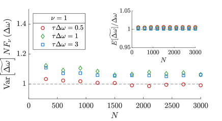
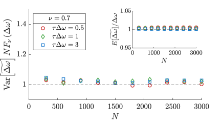
Figure 4: Simulation of the variance normalized with respect to the Cramér-Rao bound for $\nu=1$ (top figure), and $\nu=0.7$ (bottom figure), for values of $\tau\Delta\omega=0.5,1,3$, respectively represented with a circle, a rhombus and a square marker. In the inset it is shown the simulation of the Expected value of $\Delta\omega$ normalized. The simulation has been executed by repeating for each point the measure process $10^{4}$ times. It is possible to show that even for an amount of data $N\sim 10^{3}$ the Cramér-Rao bound is saturated, and the bias is inferior to the $1\%$.

In this section, we compare the effectiveness of this protocol with the one of a sensing scheme that does not resolve the time delay of the photons, as in Fabre and Felicetti (2021). In case of a Gaussian distribution in time for both photons, the Fisher information for non-resolving time delay measurements and unit detector precision is

$$F^{G,NR}_{\nu}\left(\Delta\omega\right)=\frac{4\nu^{2}\tau^{4}\Delta\omega^{2}}{\mathrm{e}^{2\tau^{2}\Delta\omega^{2}}-\nu^{2}}=H\left(\Delta\omega\right)\frac{2\nu^{2}\tau^{2}\Delta\omega^{2}}{\mathrm{e}^{2\tau^{2}\Delta\omega^{2}}-\nu^{2}}.$$ (12)

Both $F^{G}_{\nu}\left(\Delta\omega\right)$ and $F^{G,NR}_{\nu}\left(\Delta\omega\right)$ are represented in FIG. 5 as a function of $1/\tau\Delta\omega$ for different values of $\nu$ and for $\gamma=1$. It is possible to show that, due to the convexity of the Fisher information, $F^{G}_{\nu}\left(\Delta\omega\right)\geq F^{G,NR}_{\nu}\left(\Delta\omega\right)$. For $\tau\Delta\omega\ll 1$, $F^{G,NR}_{\nu}\left(\Delta\omega\right)$ approaches $F^{G}_{\nu}\left(\Delta\omega\right)$ and in particular, for $\nu=1$, the sensitivities of the resolving and non-resolving schemes are equal.

In the case of $\tau\Delta\omega\gg 1$, i.e. the case in which the photons do not overlap in their frequency distribution, the Fisher information of the resolving sensing scheme is proportional to the quantum Fisher information by a factor that depends only on $\nu$ and $\gamma$. In this case, as shown in Appendix C,

$$F_{\nu}\left(\Delta\omega\right)=\gamma^{2}\left(1-\sqrt{1-\nu^{2}}\right)F_{\nu=1}\left(\Delta\omega\right).$$ (13)

Instead, the Fisher information of the non-resolving sensing scheme cannot retrieve any information about $\Delta\omega$ for $\tau\Delta\omega\gg 1$.

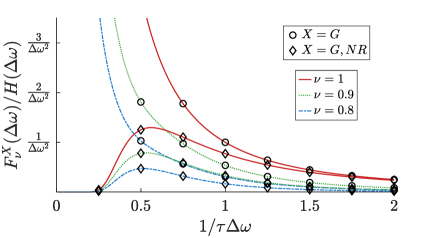
Figure 5: Plot of Fisher informations $F_{\nu}^{G}\left(\Delta\omega\right)$ in eq. (11) and $F_{\nu}^{G,NR}\left(\Delta\omega\right)$ in eq. (12) vs $1/\Delta\omega$, for different values of the parameter $\nu=1,0.9,0.8$. The non resolving Fisher information reaches the Quantum Cramér-Rao bound at $\nu=1$ and for $\Delta\omega\ll 1/\tau$. Instead, for $\Delta\omega\gg 1/\tau$, the non-resolving approach cannot retrieve any information of the parameter $\Delta\omega$.

VI Conclusion

We demonstrate the efficiency of an interferometric scheme based on time-resolving sampling measurements for the estimation of the frequency shift $\Delta\omega$ of two photons. We show that in the regime of $N\sim 1000$ the Cramér-Rao bound is approximately saturated and the bias is inferior to $1\%$ of the value of $\Delta\omega$, independently of the overlap between the photons and $\Delta\omega$ itself.

In fact, the efficiency of the detection does not depend on $\Delta\omega$. This is more evident when the sensing scheme is compared with a non-resolving interferometric technique, which is not efficient for large values of $\Delta\omega$. Instead, the precision of the estimation is dependent on the coherence time of the photons. That makes the precision virtually without an upper limit, especially considering techniques that can increase the coherence time of the photons.

Furthermore, this technique is not constrained by the detector frequency resolution required to directly measure the difference in frequency between the two photons. Instead, it is dependent on the efficiency of the detector in time. However, this requirement is considered only for imposing the photons indistinguishability at the detector. Having only this constraint in the detection allows us to outperform the standard spectrometers on a broader range.

Appendix A Evaluation of the probabilities in eq. (3)

A.1 Evaluation of $G\left(2\right)$

In this section we evaluate the probabilities in eq (3) of having bunching or coincidence in the sensing scheme in FIG.1 by using the correlation function

$$G^{\left(2\right)}_{C_{1}C_{2}}\left(\alpha_{1},t_{1};\alpha_{2},t_{2}\right)=\left\langle\bm{\psi}\right|\hat{E}_{C_{1}}(t_{1})^{-\left(\alpha_{1}\right)}\hat{E}_{C_{2}}(t_{2})^{-\left(\alpha_{2}\right)}\hat{E}_{C_{1}}(t_{1})^{+\left(\alpha_{1}\right)}\hat{E}_{C_{2}}(t_{2})^{+\left(\alpha_{2}\right)}\left|\bm{\psi}\right\rangle.$$ (14)

Here, the state $\left|\bm{\psi}\right\rangle$ correspond to the input state in eq. (1), that we rewrite below for clarity:

$$\left|\bm{\psi}\right\rangle=\int_{\mathbb{R}^{2}}dt^{\prime}_{1}dt^{\prime}_{2}\psi_{1}\left(t^{\prime}_{1}\right)\psi_{2}\left(t^{\prime}_{2}\right)\hat{a}^{\dagger}_{1}(t^{\prime}_{1})\hat{b}^{\dagger}_{2}(t^{\prime}_{2})\left|0\right\rangle,$$ (15)

with $\psi_{i}\left(t\right)=\left|\psi\left(t\right)\right|\mathrm{e}^{-i\omega_{i}t}$. Also, $C_{1},C_{2}$ are respectively the first and the second output of the beam splitter; $t_{1}$ and $t_{2}$ are the time of detection of each photon; $\alpha_{1},\alpha_{2}$ represent the orthogonal modes in which the two photons can be, i.e. $\hat{a}^{\dagger},\hat{d}^{\dagger}$, such that $\hat{b}^{\dagger}=\sqrt{\nu}\hat{a}^{\dagger}+\sqrt{1-\nu}\hat{d}^{\dagger}$. We write the field operators in the following way

$$\begin{split}\hat{E}_{C_{1}}(t_{1})^{+\left(\alpha\right)}&=\sum_{S=1,2}\frac{\mathrm{e}^{i\Phi\left(S,C_{1}\right)}}{\sqrt{2}}\hat{\alpha}_{s}(t_{1})=\sum_{S=1,2}\hat{E}_{sC_{1}}(t_{1})^{+\left(\alpha\right)}\qquad,\qquad\hat{\alpha}=\hat{a},\hat{d};\left(\hat{E}_{C_{1}}(t_{1})^{+\left(\alpha\right)}\right)^{\dagger}=\hat{E}_{C_{1}}(t_{1})^{-\left(\alpha\right)},\end{split}$$ (16)

where $s$ represents the s-th photon associated to the s-th input of the sensing scheme and $\phi$ is the phase acquired to the beam splitter.

Since $\left|\bm{\psi}\right\rangle$ is a two photon state and $\hat{E}_{C_{1}}(t_{1})^{+\left(\alpha_{1}\right)}\hat{E}_{C_{2}}(t_{2})^{+\left(\alpha_{2}\right)}$ annihilates two photon, $\hat{E}_{C_{1}}(t_{1})^{+\left(\alpha_{1}\right)}\hat{E}_{C_{2}}(t_{2})^{+\left(\alpha_{2}\right)}\left|\bm{\psi}\right\rangle\propto\left|0\right\rangle$. Similarly, $\left\langle\bm{\psi}\right|\hat{E}_{C_{1}}(t_{1})^{-\left(\alpha_{1}\right)}\hat{E}_{C_{2}}(t_{2})^{-\left(\alpha_{2}\right)}\propto\left\langle 0\right|$. So, by expanding the eq. (14) by using the eq. (16) we can write

$$\begin{split}G^{\left(2\right)}_{C_{1}C_{2}}\left(\alpha_{1},t_{1};\alpha_{2},t_{2}\right)&=\sum_{S_{i}=1,2}\left\langle\bm{\psi}\right|\hat{E}_{s_{1}C_{1}}(t_{1})^{-\left(\alpha_{1}\right)}\hat{E}_{s_{2}C_{2}}(t_{2})^{-\left(\alpha_{2}\right)}\left|0\right\rangle\left\langle 0\right|\hat{E}_{s_{3}C_{1}}(t_{1})^{+\left(\alpha_{1}\right)}\hat{E}_{s_{4}C_{2}}(t_{2})^{+\left(\alpha_{2}\right)}\left|\bm{\psi}\right\rangle=\\ &=\sum_{S_{i}=1,2}G^{\left(2\right)}_{S_{1}S_{2}S_{3}S_{4}C_{1}C_{2}}.\end{split}$$ (17)

By considering that the two input photons are in two different channels, this equation allows us to show that

$$\begin{split}G^{\left(2\right)}_{11S_{3}S_{4}C_{1}C_{2}}=G^{\left(2\right)}_{22S_{3}S_{4}C_{1}C_{2}}=G^{\left(2\right)}_{S_{1}S_{2}11C_{1}C_{2}}=G^{\left(2\right)}_{S_{1}S_{2}22C_{1}C_{2}}=0,\end{split}$$ (18)

therefore,

$$\begin{split}G^{\left(2\right)}_{C_{1}C_{2}}\left(\alpha_{1},t_{1};\alpha_{2},t_{2}\right)&=\sum_{S_{1},S_{2}=1,2}G^{\left(2\right)}_{S_{1}\sigma\left(S_{1}\right)S_{2}\sigma\left(S_{2}\right)C_{1}C_{2}}\qquad,\qquad\sigma\left(1\right)=2,\sigma\left(2\right)=1.\end{split}$$ (19)

We can rewrite the four remaining terms of the sum in a simpler form, that is

$$\begin{split}G^{\left(2\right)}_{C_{1}C_{2}}\left(\alpha_{1},t_{1};\alpha_{2},t_{2}\right)&=\left|\sum_{S_{1}=1,2}\left\langle 0\right|\hat{E}_{s_{1}C_{1}}(t_{1})^{+\left(\alpha_{1}\right)}\hat{E}_{\sigma\left(S_{1}\right)C_{2}}(t_{2})^{+\left(\alpha_{2}\right)}\left|\bm{\psi}\right\rangle\right|^{2}.\end{split}$$ (20)

By using eq. (15) and eq. (16), we can expand each term as follows:

$$\begin{split}\left\langle 0\right|\hat{E}_{s_{1}C_{1}}(t_{1})^{+\left(\alpha\right)}\hat{E}_{\sigma\left(S_{1}\right)C_{2}}(t_{2})^{+\left(\beta\right)}\left|\bm{\psi}\right\rangle&=\frac{1}{2}\int_{\mathbb{R}^{2}}dt^{\prime}_{1}dt^{\prime}_{2}\mathrm{e}^{i\Phi\left(S_{1},C_{1}\right)}\mathrm{e}^{i\Phi\left(\sigma\left(S_{1}\right),C_{2}\right)}\times\\ &\times\psi_{1}\left(t^{\prime}_{1}\right)\psi_{2}\left(t^{\prime}_{2}\right)\left\langle 0\right|\hat{\alpha}_{s_{1}}(t_{1})\hat{\beta}_{\sigma\left(S_{1}\right)}(t_{2})\hat{a}^{\dagger}_{1}(t^{\prime}_{1})\hat{b}^{\dagger}_{2}(t^{\prime}_{2})\left|0\right\rangle.\end{split}$$ (21)

By remembering that $\hat{a}^{\dagger}$ is orthogonal to $\hat{d}^{\dagger}$ and that $\hat{b}^{\dagger}=\sqrt{\nu}\hat{a}^{\dagger}+\sqrt{1-\nu}\hat{d}^{\dagger}$, we can find that the null terms are the following:

$$\begin{split}&\left\langle 0\right|\hat{E}_{s_{1}C_{1}}(t_{1})^{+\left(d\right)}\hat{E}_{\sigma\left(S_{1}\right)C_{2}}(t_{2})^{+\left(d\right)}\left|\bm{\psi}\right\rangle=0,\\ &\left\langle 0\right|\hat{E}_{2C_{1}}(t_{1})^{+\left(a\right)}\hat{E}_{1C_{2}}(t_{2})^{+\left(d\right)}\left|\bm{\psi}\right\rangle=0,\\ &\left\langle 0\right|\hat{E}_{1C_{1}}(t_{1})^{+\left(d\right)}\hat{E}_{2C_{2}}(t_{2})^{+\left(a\right)}\left|\bm{\psi}\right\rangle=0,\\ \end{split}$$ (22)

The non-zero terms, instead, assume the forms

$$\begin{split}\left\langle 0\right|\hat{E}_{1C_{1}}(t_{1})^{+\left(a\right)}\hat{E}_{2C_{2}}(t_{2})^{+\left(d\right)}\left|\bm{\psi}\right\rangle&=\frac{1}{2}\int_{\mathbb{R}^{2}}dt^{\prime}_{1}dt^{\prime}_{2}\mathrm{e}^{i\Phi\left(1,C_{1}\right)}\mathrm{e}^{i\Phi\left(2,C_{2}\right)}\times\\ &\times\psi_{1}\left(t^{\prime}_{1}\right)\psi_{2}\left(t^{\prime}_{2}\right)\left\langle 0\right|\hat{a}_{1}(t_{1})\hat{d}_{2}(t_{2})\hat{a}^{\dagger}_{1}(t^{\prime}_{1})\hat{b}^{\dagger}_{2}(t^{\prime}_{2})\left|0\right\rangle=\\ &=\frac{\sqrt{1-\nu}}{2}\mathrm{e}^{i\Phi\left(1,C_{1}\right)}\mathrm{e}^{i\Phi\left(2,C_{2}\right)}\psi_{1}\left(t_{1}\right)\psi_{2}\left(t_{2}\right),\end{split}$$ (23)

$$\begin{split}\left\langle 0\right|\hat{E}_{2C_{1}}(t_{1})^{+\left(d\right)}\hat{E}_{1C_{2}}(t_{2})^{+\left(a\right)}\left|\bm{\psi}\right\rangle&=\frac{1}{2}\int_{\mathbb{R}^{2}}dt^{\prime}_{1}dt^{\prime}_{2}\mathrm{e}^{i\Phi\left(2,C_{1}\right)}\mathrm{e}^{i\Phi\left(1,C_{2}\right)}\times\\ &\times\psi_{1}\left(t^{\prime}_{1}\right)\psi_{2}\left(t^{\prime}_{2}\right)\left\langle 0\right|\hat{d}_{2}(t_{1})\hat{a}_{1}(t_{2})\hat{a}^{\dagger}_{1}(t^{\prime}_{1})\hat{b}^{\dagger}_{2}(t^{\prime}_{2})\left|0\right\rangle=\\ &=\frac{\sqrt{1-\nu}}{2}\mathrm{e}^{i\Phi\left(1,C_{1}\right)}\mathrm{e}^{i\Phi\left(2,C_{2}\right)}\psi_{1}\left(t_{2}\right)\psi_{2}\left(t_{1}\right),\end{split}$$ (24)

$$\begin{split}\left\langle 0\right|\hat{E}_{s_{1}C_{1}}(t_{1})^{+\left(a\right)}\hat{E}_{\sigma\left(S_{1}\right)C_{2}}(t_{2})^{+\left(a\right)}\left|\bm{\psi}\right\rangle&=\frac{1}{2}\int_{\mathbb{R}^{2}}dt^{\prime}_{1}dt^{\prime}_{2}\mathrm{e}^{i\Phi\left(S_{1},C_{1}\right)}\mathrm{e}^{i\Phi\left(\sigma\left(S_{1}\right),C_{2}\right)}\times\\ &\times\psi_{1}\left(t^{\prime}_{1}\right)\psi_{2}\left(t^{\prime}_{2}\right)\left\langle 0\right|\hat{d}_{s_{1}}(t_{1})\hat{a}_{\sigma\left(S_{1}\right)}(t_{2})\hat{a}^{\dagger}_{1}(t^{\prime}_{1})\hat{b}^{\dagger}_{2}(t^{\prime}_{2})\left|0\right\rangle=\\ &=\frac{\sqrt{\nu}}{2}\Big{(}\delta_{1S_{1}}\mathrm{e}^{i\Phi\left(1,C_{1}\right)}\mathrm{e}^{i\Phi\left(2,C_{2}\right)}\psi_{1}\left(t_{1}\right)\psi_{2}\left(t_{2}\right)+\\ &+\delta_{2S_{1}}\mathrm{e}^{i\Phi\left(2,C_{1}\right)}\mathrm{e}^{i\Phi\left(1,C_{2}\right)}\psi_{1}\left(t_{2}\right)\psi_{2}\left(t_{1}\right)\Big{)}.\end{split}$$ (25)

Using these results in eq. (20), all the second-order correlation functions are

$$\begin{split}G^{\left(2\right)}_{C_{1}C_{2}}\left(d,t_{1};d,t_{2}\right)&=0,\\ G^{\left(2\right)}_{C_{1}C_{2}}\left(a,t_{1};d,t_{2}\right)&=G^{\left(2\right)}_{C_{1}C_{2}}\left(d,t_{1};a,t_{2}\right)=\frac{1-\nu}{4}\left|\psi\left(t_{2}\right)\psi\left(t_{1}\right)\right|^{2},\\ G^{\left(2\right)}_{C_{1}C_{2}}\left(a,t_{1};a,t_{2}\right)&=\frac{\nu}{4}\left|\psi\left(t_{2}\right)\psi\left(t_{1}\right)\right|^{2}\left|\mathrm{e}^{i\Phi\left(1,C_{1}\right)+i\Phi\left(2,C_{2}\right)}\mathrm{e}^{-i\omega_{1}t_{1}-i\omega_{2}t^{\prime}_{2}}+\mathrm{e}^{i\Phi\left(2,C_{1}\right)+i\Phi\left(1,C_{2}\right)}\mathrm{e}^{-i\omega_{1}t^{\prime}_{2}-i\omega_{2}t_{1}}\right|^{2}=\\ &=\frac{\nu}{2}\left|\psi\left(t_{2}\right)\psi\left(t_{1}\right)\right|^{2}\left(1+\mathrm{Re\left(\mathrm{e}^{i\left[\Phi\left(1,C_{1}\right)+\Phi\left(2,C_{2}\right)-\Phi\left(2,C_{1}\right)-\Phi\left(1,C_{2}\right)\right]}\mathrm{e}^{i\Delta\omega\Delta t}\right)}\right)=\\ &=\frac{\nu}{2}\left|\psi\left(t_{2}\right)\psi\left(t_{1}\right)\right|^{2}\left(1+\left(2\delta_{C_{1}C_{2}}-1\right)\cos\Delta\omega\Delta t\right),\end{split}$$ (26)

where $\Phi\left(1,C_{1}\right)+\Phi\left(2,C_{2}\right)-\Phi\left(2,C_{1}\right)-\Phi\left(1,C_{2}\right)=\pm\pi$ in case of coincidence event ($C_{1}\neq C_{2}$) and it is equal to 0 in case of a bunching event ($C_{1}=C_{2}$).

A.2 Evaluation of the probabilities

After evaluating the second-order correlation functions we can retrieve the probabilities of coincidence (labelled with $A$) and bunching (labelled with $B$) as follows:

$$\begin{split}P_{\nu}\left(t_{1},t_{2},A|\Delta\omega\right)&=\sum_{\alpha,\beta=a,d}G^{\left(2\right)}_{12}\left(\alpha,t_{1};\beta,t_{2}\right)=\frac{1}{2}\left|\psi\left(t_{2}\right)\psi\left(t_{1}\right)\right|^{2}\left(1-\nu\cos\Delta\omega\Delta t\right),\\ P_{\nu}\left(t_{1},t_{2},B|\Delta\omega\right)&=\frac{1}{2}\sum_{\alpha,\beta=a,d}G^{\left(2\right)}_{11}\left(\alpha,t_{1};\beta,t_{2}\right)+G^{\left(2\right)}_{22}\left(\alpha,t_{1};\beta,t_{2}\right)=\frac{1}{2}\left|\psi\left(t_{2}\right)\psi\left(t_{1}\right)\right|^{2}\left(1+\nu\cos\Delta\omega\Delta t\right),\end{split}$$ (27)

where the factor $1/2$ is used for taking into account the symmetry $t_{2}\leftrightarrow t_{1}$. Since the sensing protocol is designed for detecting only the time delay, we can define $\tau_{tot}=t_{1}+t_{2}$ and $\Delta t=t_{2}-t_{1}$, and we can integrate the probabilities over $\tau_{tot}$, obtaining

$$P_{\nu}\left(\Delta t,X|\Delta\omega\right)=\int_{\mathbb{R}}d\tau_{tot}P_{\nu}\left(\frac{\tau_{tot}-\Delta t}{2},\frac{\tau_{tot}+\Delta t}{2},X\right),\qquad X=A,B.$$ (28)

By solving the integral, the probabilities in eq (3) are,

$$P_{\nu}\left(\Delta t,X|\Delta\omega\right)=\frac{C\left(\Delta t\right)}{2}\left(1+\nu\alpha\left(X\right)\cos\left(\Delta\omega\Delta t\right)\right),\qquad X=A,B,$$ (29)

where $C\left(\Delta t\right)$ is the envelope defined as follows:

$$C\left(\Delta t\right)=\int_{\mathbb{R}}d\tau_{tot}\left|\psi\left(\frac{\tau_{tot}-\Delta t}{2}\right)\psi\left(\frac{\tau_{tot}+\Delta t}{2}\right)\right|^{2}.$$ (30)

If we take into account the efficiency of the detectors $\gamma\in\left[0,1\right]$ (which is the same for both the detectors), it is possible to register events where 0 photons or only one photon is detected. By defining these probabilities respectively as $P_{0}$ and $P_{1}$ and by using eq. (27), we can write

$$\begin{cases}&P_{0}=\left(1-\gamma\right)^{2}\\ &P_{1}\left(t_{1}\right)=\gamma\left(1-\gamma\right)\int_{\mathbb{R}}dt_{2}\left(P_{\nu}\left(t_{1},t_{2},A\right)+P_{\nu}\left(t_{1},t_{2},B\right)\right)\\ &P\left(t_{1},t_{2},X\right)=\gamma^{2}P_{\nu}\left(t_{1},t_{2},X\right),\qquad X=A,B\end{cases}.$$ (31)

Therefore, integrating with respect to $\tau_{tot}$, the probabilities become

$$\begin{cases}&P_{0}=\left(1-\gamma\right)^{2}\\ &P_{1}\left(\Delta t\right)=2\gamma\left(1-\gamma\right)\int d\tau_{tot}\left|\psi\left(t_{1}\right)\right|^{2}=2\gamma\left(1-\gamma\right)\\ &P\left(\Delta t.X|\Delta\omega\right)=\gamma^{2}P_{\nu}\left(\Delta t.X|\Delta\omega\right),\qquad X=A,B\end{cases}.$$ (32)

Here, the one-photon event and the zero-photons event have a probability that depends only to the efficiency of the detectors. The two-photons event has a probability that is proportional to the square of the efficiency.

Appendix B Evaluation of the quantum Fisher information in eq. 6 and eq. 7

In this section we evaluate the quantum Fisher information $H$ for the estimation of $\Delta\omega=\omega_{2}-\omega_{1}$ that is encoded in the input state $\left|\bm{\psi}\right\rangle$ defined in eq (15). In order to do that, we evaluate first the quantum Fisher information for the single parameters $\omega_{1}$ and $\omega_{2}$. Each photon encode respectively of these parameter. We define for the i-th photon the single-photon state $\left|\psi_{i}\right\rangle$, $i=1,2$, such that $\left|\bm{\psi}\right\rangle=\left|\psi_{1}\right\rangle\otimes\left|\psi_{2}\right\rangle$, where

$$\begin{split}\left|\psi_{1}\right\rangle=&\int_{\mathbb{R}}dt^{\prime}_{1}\left|\psi\left(t^{\prime}_{1}\right)\right|\mathrm{e}^{-i\omega_{1}t^{\prime}_{1}}\hat{a}^{\dagger}_{1}(t^{\prime}_{1})\left|0\right\rangle,\\ \left|\psi_{2}\right\rangle=&\int_{\mathbb{R}}dt^{\prime}_{2}\left|\psi\left(t^{\prime}_{2}\right)\right|\mathrm{e}^{-i\omega_{2}t^{\prime}_{2}}\hat{b}^{\dagger}_{2}(t^{\prime}_{2})\left|0\right\rangle.\end{split}$$ (33)

therefore, the quantum Fisher information is the sum of two matrices, i.e. $H=H_{1}+H_{2}$, where

$$H_{i}\left(\omega_{1},\omega_{2}\right)=4\mathrm{Re}\left(\left\langle\partial_{x}\psi_{i}|\partial_{x}\psi_{i}\right\rangle-\left|\left\langle\psi_{i}|\partial_{x}\psi_{i}\right\rangle\right|^{2}\right),\qquad x=\omega_{1},\omega_{2}.$$ (34)

Since each photon encode only one parameter, $\left|\partial_{\omega_{2}}\psi_{1}\right\rangle=\left|\partial_{\omega_{1}}\psi_{2}\right\rangle=0$. Therefore, the quantum Fisher information will be diagonal:

$$H\left(\omega_{1},\omega_{2}\right)=\begin{pmatrix}H_{1}\left(\omega_{1}\right)&0\\ 0&H_{2}\left(\omega_{2}\right)\end{pmatrix}.$$ (35)

We find the i-th diagonal term by using $\left|\psi_{i}\right\rangle$ in eq. (33) and $\left|\partial_{\omega_{i}}\psi_{i}\right\rangle$, as shown in eq (34). The kets $\left|\partial_{\omega_{i}}\psi_{i}\right\rangle$ are the following:

$$\begin{split}\left|\partial_{\omega_{1}}\psi_{1}\right\rangle=&-i\int_{\mathbb{R}}dt^{\prime}_{1}t^{\prime}_{1}\left|\psi\left(t^{\prime}_{1}\right)\right|\mathrm{e}^{-i\omega_{1}t^{\prime}_{1}}\hat{a}^{\dagger}_{1}(t^{\prime}_{1})\left|0\right\rangle,\\ \left|\partial_{\omega_{2}}\psi_{2}\right\rangle=&-i\int_{\mathbb{R}}dt^{\prime}_{2}t^{\prime}_{2}\left|\psi\left(t^{\prime}_{2}\right)\right|\mathrm{e}^{-i\omega_{2}t^{\prime}_{2}}\hat{b}^{\dagger}_{2}(t^{\prime}_{2})\left|0\right\rangle.\end{split}$$ (36)

So, by using the eqs. (33), (34) and (36), we find the i-th diagonal term of the quantum Fisher information

$$H_{i}\left(\omega_{i}\right)=4\left(\int_{\mathbb{R}}dt_{i}\left|t_{i}\psi\left(t_{i}\right)\right|^{2}-\left|\int_{\mathbb{R}}dt_{i}t_{i}\left|\psi\left(t_{i}\right)\right|^{2}\right|^{2}\right)=4\tau^{2},$$ (37)

where $\tau$ is the variance of the temporal distribution $\left|\psi\left(t\right)\right|^{2}$ of each photon. Thus the quantum Fisher information for the parameters $\omega_{1}$ and $\omega_{2}$ assumes the form

$$H\left(\omega_{1},\omega_{2}\right)=4\tau^{2}I,$$ (38)

where $I$ is the $2\times 2$ identity matrix. For evaluating the quantum Fisher information for $\Delta\omega$, we define $\omega_{M}=\omega_{1}+\omega_{2}$. We evaluate the quantum Fisher information for $\left(\omega_{M},\Delta\omega\right)$ by applying a transformation on $H$ with the Jacobian

$$J=\frac{1}{2}\begin{pmatrix}1&1\\ 1&-1\end{pmatrix}$$ (39)

in the following way:

$$H\left(\omega_{M},\Delta\omega\right)=JH\left(\omega_{1},\omega_{2}\right)J^{T}=\tau^{2}\begin{pmatrix}1&1\\ 1&-1\end{pmatrix}\begin{pmatrix}1&0\\ 0&1\end{pmatrix}\begin{pmatrix}1&1\\ 1&-1\end{pmatrix}=2\tau^{2}I.$$ (40)

This quantum Fisher information proves that it is possible to estimate separately $\omega_{M}$ and $\Delta\omega$, and that the quantum Fisher information for $\Delta\omega$ is $H\left(\Delta\omega\right)=2\tau^{2}$.

Appendix C Evaluation of the Fisher information

C.1 Fisher information in eq. 9

In this section we evaluate the Fisher information starting from its definition

$$\begin{split}F_{\nu}\left(\Delta\omega\right)&=E\left[\left(\frac{\partial}{\partial\Delta\omega}\log P_{\nu}\left(\Delta t,X|\Delta\omega\right)\right)^{2}\right].\end{split}$$ (41)

Here, by using the probabilities formula in eq 3, we find that

$$\begin{split}F_{\nu}\left(\Delta\omega\right)&=\sum_{X=A,B}\int_{\mathbb{R}}d\Delta t\frac{1}{P_{\nu}\left(\Delta t,X|\Delta\omega\right)}\left(\frac{\partial}{\partial\Delta\omega}P_{\nu}\left(\Delta t,X|\Delta\omega\right)\right)^{2}=\\ &=\nu^{2}\int_{\mathbb{R}}d\Delta tC\left(\Delta t\right)\frac{\Delta t^{2}\sin^{2}\left(\Delta\omega\Delta t\right)}{1-\nu^{2}\cos^{2}\left(\Delta\omega\Delta t\right)}=\int_{\mathbb{R}}d\Delta tC\left(\Delta t\right)\Delta t^{2}\beta_{\nu}\left(\Delta\omega\Delta t\right),\end{split}$$ (42)

where we define the function $\beta_{\nu}\left(\Delta\omega\Delta t\right)$ as follows:

$$\beta_{\nu}\left(\Delta\omega\Delta t\right)=\frac{\nu^{2}\sin^{2}\left(\Delta\omega\Delta t\right)}{1-\nu^{2}\cos^{2}\left(\Delta\omega\Delta t\right)}.$$ (43)

It is worth to notice that for $\nu=1$, $\beta_{\nu}=1\left(\Delta\omega\Delta t\right)=1$. So, in this case the Fisher information assumes the form

$$F_{\nu=1}\left(\Delta\omega\right)=\int_{\mathbb{R}}d\Delta t\Delta t^{2}C\left(\Delta t\right)=2\tau^{2}=H\left(\Delta\omega\right).$$ (44)

Therefore, for $\nu=1$, the fisher information saturates the quantum Cramér-Rao bound, and the maximum precision is achieved.

C.2 For $\tau\Delta\omega\gg 1$

the Fisher information assumes a simpler form in the regime $\tau\Delta\omega\gg 1$. In fact, in this regime, we can approximate the value of the Fisher information by splitting the interval of integration in eq. (42) in intervals of length $\pi/\Delta t$. In each of this intervals, the term $C\left(\Delta t\right)\Delta t^{2}$ can be considered approximately constant, and thus we can substitute it with a constant value:

$$F_{\nu}\left(\Delta\omega\right)\simeq\sum_{n\in\mathbb{Z}}\left(\frac{\pi n}{\Delta\omega}\right)^{2}C\left(\frac{\pi n}{\Delta\omega}\right)\int_{\frac{n\pi}{\Delta\omega}}^{\frac{\left(n+1\right)\pi}{\Delta\omega}}d\Delta t\beta_{\nu}\left(\Delta\omega\Delta t\right)=\sum_{n\in\mathbb{Z}}\left(\frac{\pi n}{\Delta\omega}\right)^{2}C\left(\frac{\pi n}{\Delta\omega}\right)\frac{\Delta\omega}{\pi}\bar{\beta}_{\nu},$$ (45)

where $\bar{\beta}_{\nu}$ is the mean of the function $\beta_{\nu}\left(x\right)$ in each interval:

$$\begin{split}\bar{\beta}_{\nu}=\frac{\Delta\omega}{\pi}\int_{0}^{\frac{\pi}{\Delta\omega}}d\Delta t\beta_{\nu}\left(\Delta\omega\Delta t\right)=\frac{1}{\pi}\int_{0}^{\pi}dx\beta_{\nu}\left(x\right)=1-\sqrt{1-\nu^{2}}.\end{split}$$ (46)

By summing again all the terms of the Fisher information in eq (45), we can rewrite the Fisher information as an integral, by using the approximations $\sum_{n\in\mathbb{Z}}\frac{\Delta\omega}{\pi}\bar{\beta}_{\nu}\rightarrow\int_{\mathbb{R}}d\xi$ and $\left(\frac{\pi n}{\Delta\omega}\right)^{2}C\left(\frac{\pi n}{\Delta\omega}\right)\rightarrow C\left(\xi\right)\xi^{2}$,

$$F_{\nu}\left(\Delta\omega\right)\simeq\bar{\beta}_{\nu}\int_{\mathbb{R}}d\xi C\left(\xi\right)\xi^{2}=2\tau^{2}\bar{\beta}_{\nu}.$$ (47)

In this way we prove that in the regime $\tau\Delta\omega\gg 1$, the Fisher information is proportional to the quantum Fisher information by a function of only $\nu$.

C.3 Fisher information in eq. 11

If the distribution in time of the two input photons $\left|\psi\left(t\right)\right|^{2}$ is Gaussian, we can show that the envelope in eq. 30 can be expressed as follows:

$$C\left(\Delta t\right)=\frac{1}{\sqrt{4\pi\tau^{2}}}\mathrm{exp}\left[-\frac{\Delta t}{4\tau^{2}}\right].$$ (48)

Therefore, by substituting $\Delta t/2\tau\rightarrow\kappa$ in eq (42), we found that the Fisher information for Gaussian photons in time is

$$\begin{split}F^{G}_{\nu}\left(\Delta\omega\right)=\frac{4\tau^{2}}{\sqrt{\pi}}\int_{\mathbb{R}}d\kappa\mathrm{e}^{-\kappa^{2}}\kappa^{2}\beta_{\nu}\left(2\tau\Delta\omega\kappa\right)\Rightarrow\frac{F_{\nu}\left(\Delta\omega\right)}{H\left(\Delta\omega\right)}=\frac{2}{\sqrt{\pi}}\int_{\mathbb{R}}d\kappa\mathrm{e}^{-\kappa^{2}}\kappa^{2}\beta_{\nu}\left(2\tau\Delta\omega\kappa\right).\end{split}$$ (49)

C.4 Fisher information in eq. 12

If the detectors at the output of the beam splitter represented in fig.1 do not resolve the time delay, the output can be only of two types: bunching and coincidence. We find their probabilities by integrating with respect to $\Delta t$ the probabilities in eq. (29):

$$P\left(X|\Delta\omega\right)=\int_{\mathbb{R}}d\Delta tP_{\nu}\left(X,\Delta t|\Delta\omega\right)=\frac{1}{2}+\frac{\nu\alpha\left(X\right)}{2}\int_{\mathbb{R}}d\Delta tC\left(\Delta t\right)\cos^{2}\left(\Delta t\Delta\omega\right),\qquad X=A,B.$$ (50)

In particular, if the photons are Gaussian in time, by using eq. (48), we find that

$$P\left(X|\Delta\omega\right)=\frac{1}{2}\left(1+\nu\alpha\left(X\right)\mathrm{e}^{-\tau^{2}\Delta\omega^{2}}\right),\qquad X=A,B.$$ (51)

We evaluate the Fisher information using its definition, that here is written for clarity:

$$\begin{split}F^{G,NR}_{\nu}\left(\Delta\omega\right)&=E\left[\left(\frac{\partial}{\partial\Delta\omega}\log P_{\nu}\left(X|\Delta\omega\right)\right)^{2}\right].\end{split}$$ (52)

Therefore, by using eq. (51), the Fisher information assumes the form

$$\begin{split}F^{G,NR}_{\nu}\left(\Delta\omega\right)&=\sum_{X=A,B}\frac{1}{P_{\nu}\left(X|\Delta\omega\right)}\left(\frac{\partial P_{\nu}\left(X|\Delta\omega\right)}{\partial\Delta\omega}\right)^{2}=\\ &=\frac{4\nu^{2}\tau^{4}\Delta\omega^{2}}{\mathrm{e}^{2\tau^{2}\Delta\omega^{2}}-\nu^{2}}=H\left(\Delta\omega\right)\frac{2\nu^{2}\tau^{2}\Delta\omega^{2}}{\mathrm{e}^{2\tau^{2}\Delta\omega^{2}}-\nu^{2}}.\end{split}$$ (53)

For $\tau\Delta\omega\ll 1$ we can simplify it by substituting $\mathrm{e}^{2\tau^{2}\Delta\omega^{2}}\rightarrow 1+2\tau^{2}\Delta\omega^{2}$. In this case, the Fisher information becomes equal to the Quantum Fisher information:

$$F^{G,NR}_{\nu}=1\left(\Delta\omega\right)=2\tau^{2}=H\left(\Delta\omega\right).$$ (54)