Machine Learning Neutrino-Nucleus Cross Sections

Abstract

Neutrino-nucleus scattering cross sections are critical theoretical inputs for long-baseline neutrino oscillation experiments. However, robust modeling of these cross sections remains challenging. For a simple but physically motivated toy model of the DUNE experiment, we demonstrate that an accurate neural-network model of the cross section—leveraging Standard Model symmetries—can be learned from near-detector data. We then perform a neutrino oscillation analysis with simulated far-detector events, finding that the modeled cross section achieves results consistent with what could be obtained if the true cross section were known exactly. This proof-of-principle study highlights the potential of future neutrino near-detector datasets and data-driven cross-section models.

Neutrinos serve as an excellent probe of the Standard Model and what lies beyond. After decades of extensive effort, neutrino physics is now entering a precision era, with next-generation experiments aiming to measure mixing parameters to percent-level accuracy [1, 2, 3]. Consequently, the precision required for relevant theoretical inputs has significantly increased. A prominent example is the neutrino-nucleus scattering cross section in the GeV range, which is critical as neutrino-nucleus scattering is the primary detection channel used in long-baseline accelerator-based neutrino experiments [4, 5, 6].

The primary ingredients needed to constrain neutrino oscillation parameters are incident neutrino energy distributions. However, because neutrinos are not directly observed in detectors, one typically reconstructs the incident neutrino energy of each event from the measured daughter particles [7, 8, 9, 10, 11]. This reconstruction process relies on exclusive differential cross sections [12, 13, 14, 8, 15, 16]; for example, accurate modeling of the energy of neutrons, which detectors often miss, is vital for accurately reconstructing the neutrino energy. Therefore, cross-section models encapsulated in event generators are extensively utilized in neutrino experiments [17, 18, 19, 20, 21, 22, 23].

A first-principles calculation of neutrino-nucleus scattering cross sections proves to be a significant challenge. The nuclear materials used in neutrino experiments, such as carbon, oxygen, and argon, have complex internal structures. At low energies, they can be modeled as collections of protons and neutrons described by chiral effective field theory (EFT). At high energies, they can be accurately approximated as collections of quarks and gluons with interactions described by perturbative QCD. However, at medium energies of a few GeV, which coincide with the range of accelerator neutrino beam energies, constructing a systematically improvable EFT for nuclear physics remains difficult [24, 25, 26, 27, 28, 29].

To address the challenges of cross-section modeling and other systematic uncertainties, oscillation experiments employ near detectors. By placing a detector close to the beam source—before oscillations are expected to occur—experiments can use near-detector (ND) events as validation tools for event generators. In a process called ND tuning, experiments use discrepancies between generator predictions and measured spectra to adjust generator models before using them to analyze far-detector (FD) samples [30, 9, 10, 11]. However, the accuracy of tuned cross sections relies on the validity of their underlying physics models and affects how well they can extrapolate from near- to far-detector kinematics. Significant cross-section uncertainties can still enter oscillation analyses after ND tuning [31, 30, 9, 10, 32, 11].

In this Letter, we explore an alternative approach to oscillation analysis using machine learning (ML). To establish its viability, we consider only inclusive data in this initial exploration. We construct a cross-section model using a neural network (NN) trained on mock ND data, specifically the outgoing muon energy $E_{\ell}$ and angle $\cos\theta$. We then apply our cross-section model to determine oscillation parameters by optimizing agreement between mock FD data and predicted $(E_{\ell},\cos\theta)$ distributions. There is no event-by-event neutrino energy reconstruction in our approach; only distributions of neutrino energies and $(E_{\ell},\cos\theta)$ enter both our cross-section model training and our subsequent neutrino oscillation analysis. The only theoretical assumption in our approach is that the inclusive neutrino-nucleus cross section can be parameterized by structure functions, which follows directly from Standard Model symmetries. Previous work has demonstrated that NN parameterizations can be used to accurately constrain one-dimensional parton distribution functions (PDFs) for both nucleons [33] and nuclei [34], and more recently to model lepton-nucleus cross sections using two-dimensional structure/response functions such as those considered here [35, 36, 37].

Our new approach is not meant to replace but rather complement the traditional one in several key aspects. Our cross-section model is data-driven: rather than using ND data to fine-tune the model, we build the model from the ground up using the data. This ensures our model fully exploits the power of ND samples—incredible statistics and small detector systematics. Our method also offers the flexibility of adding layers of theoretical assumptions, e.g., relations between nuclear structure functions. Conversely, our method only applies to oscillation measurements and not to general new physics searches at the ND, which is an essential component of the accelerator neutrino program [38, 39, 40, 41, 42, 43, 44, 45, 46, 47, 48, 49].

To validate our approach in this proof-of-principle study, we conduct a closure test using a toy cross-section model with known structure functions. This allows us to directly assess how well our model learns the true cross section and how this affects its ability to describe near- and far-detector flux-averaged cross sections. This closure test is a prerequisite to future studies that will apply the same approach to data, or to event generators, which will also test whether their underlying physics models admit decomposition into structure functions. We also adopt several further simplifications that can all be relaxed in future studies. First, we use only the outgoing lepton information, specifically $E_{\ell}$ and $\cos\theta$, and ignore any hadronic particles. Second, we consider only the oscillation channel $P(\nu_{\mu}\rightarrow\nu_{\mu})$ and disregard all other channels. Lastly, we do not account for any detector effects such as energy resolution and assume infinite ND statistics.

Neutrino-nucleus scattering theory — Consider charged-current scattering of a neutrino with initial energy $E_{\nu}$ on a nucleus into a final state consisting of a charged lepton with energy $E_{\ell}$ and a hadronic remnant. The inclusive cross section can be parameterized in terms of a set of five structure functions [50, 51, 52] as

$$\begin{split}&\frac{d^{2}\sigma^{(\nu A)}}{dE_{\ell}d\cos\theta}(E_{\nu})=\frac{|V_{ud}|^{2}G_{F}^{2}E_{\ell}}{\pi}\sqrt{1-\frac{m_{\ell}^{2}}{E_{\ell}^{2}}}\\ &\hskip 25.0pt\times\left\{\frac{E_{\nu}}{M_{A}}\left(1-y-\frac{Q^{2}+m_{\ell}^{2}}{4E_{\nu}^{2}}\right)W_{2}(x,Q^{2})\right.\\ &\hskip 35.0pt+\tilde{y}W_{1}(x,Q^{2})+\left(1-\frac{\tilde{y}}{2}\right)W_{3}(x,Q^{2})\\ &\hskip 35.0pt\left.-\left(\frac{m_{\ell}^{2}}{Q^{2}}\right)\left[2W_{5}(x,Q^{2})-\tilde{y}W_{4}(x,Q^{2})\right]\vphantom{\frac{M_{A}xy}{2E_{\nu}}}\right\},\end{split}$$ (1)

where $\theta$ is the lepton scattering angle, $m_{\ell}$ the charged lepton mass, $M_{A}$ the nuclear mass, $Q^{2}$ the four-momentum transfer squared, $x$ is Bjorken $x$, $y=Q^{2}/(2M_{A}E_{\nu}x)$ the inelasticity, and $\tilde{y}\equiv y(1+m_{\ell}^{2}/Q^{2})$. The nuclear structure functions $W_{i}(x,Q^{2})$ are defined from a Lorentz decomposition of $\bigl{<}A|J_{\mu}^{\dagger}J_{\nu}|A\bigr{>}$ where $J_{\mu}=\bar{u}\gamma_{\mu}(1-\gamma_{5})d$ is an electroweak current and $\bigl{|}A\bigr{>}$ is the nuclear ground state. Higher-order electroweak corrections and $\mathcal{O}(Q^{2}/m_{W}^{2})$ effects are neglected here and throughout; see Refs. [53, 54, 55] for discussion. Factors of $x$ and $Q^{2}$ have been absorbed into the $W_{i}$ to remove zeros and poles from kinematic prefactors, which facilitates NN fitting. They are related to the $F_{i}$ in Ref. [52] by $W_{i}=xF_{i}$ for $i\in\{1,3,4,5\}$ and $W_{2}=(2xM_{A}^{2}/Q^{2})F_{2}$. Cross-section contributions from $W_{4}$ and $W_{5}$ are suppressed by $m_{\ell}^{2}/Q^{2}$, which can reach 1–10% for $\sim 1$ GeV muon neutrinos and are therefore relevant for DUNE’s cross-section uncertainty targets. Global fits of the structure functions have been studied in Ref. [36].

The essential feature of Eq. (1) is that the cross section depends on three independent kinematic variables, e.g., $(E_{\nu},E_{\ell},\cos\theta)$. Inferring a three-dimensional function from the $E_{\nu}$-averaged two-dimensional distribution of $(E_{\ell},\cos\theta)$ accessible in the ND is an ill-posed problem. The benefit of the structure function parameterization is that the $W_{i}$ depend on only two independent kinematic variables, $x$ and $Q^{2}$. It is therefore possible to learn structure functions from ND data with some $(E_{\nu},x,Q^{2})$ distribution and use them to analyze FD data, as long as the ND and FD marginal distributions over $(x,Q^{2})$ are similar. For DUNE, the ND and FD $(x,Q^{2})$ distributions are expected to strongly overlap; neutrino oscillations will primarily redistribute events within the same kinematic region. This is the key physics ingredient enabling our data-driven cross-section model and oscillation analysis.

In this work, we only consider the muon neutrino charged-current channel at both the ND and FD. Without multiple distinct lepton masses, two exact degeneracies arise between the structure functions, and the cross-section can be parameterized as

$$\frac{d^{2}\sigma^{(\nu A)}}{dE_{\ell}d\cos\theta} =\frac{|V_{ud}|^{2}G_{F}^{2}E_{\ell}}{\pi}\sqrt{1-\frac{m_{\ell}^{2}}{E_{\ell}^{2}}}\left\{\frac{E_{\nu}}{M_{A}}W_{2}(x,Q^{2})\right.$$ (2)

$$\left.+W_{c}(x,Q^{2};m_{\ell}^{2})+\tilde{y}W_{y}(x,Q^{2};m_{\ell}^{2})\vphantom{\frac{M_{A}xy}{2E_{\nu}}}\right\},$$

where $W_{c}=W_{3}-Q^{2}/(2xM_{A}^{2})W_{2}-2(m_{\ell}^{2}/Q^{2})W_{5}$ and $W_{y}=W_{1}-(x/2)W_{2}-W_{3}/2+(m_{\ell}^{2}/Q^{2})W_{4}$. While not made explicit in the notation, we emphasize that the $W_{i}$ differ nontrivially between different nuclei.

Proof of principle: setup — The fundamental question we seek to address is whether the cross section can be learned well enough to extract oscillation parameters. Answering it with a closure test requires a fully known toy model of the physics of interest. To this end, we define a set of structure functions $W_{i}$, a ND flux $\Phi_{\mathrm{ND}}$, and a FD flux $\Phi_{\mathrm{FD}}$, all as explicit functions that can be evaluated for any kinematics. For simplicity, we describe these quantities as “true” or “truth” in the setting of the toy model.

For the structure functions, we take the leading order prediction from the quark-parton model [56],

$$W_{2} =\frac{4x^{2}M_{A}^{2}}{AQ^{2}}(\bar{u}+d+\bar{c}+s)\,,$$ (3)

$$W_{3} =2x(d-\bar{u}+s-\bar{c})\,,$$ (4)

with $W_{1}$ obtained using the Callan-Gross relation ($2xW_{1}=\frac{AQ^{2}}{2M_{A}^{2}}W_{2}$) [57], and $W_{4},W_{5}$ given by the tree-level relation from Ref. [50] ($2xW_{5}=\frac{AQ^{2}}{2M_{A}^{2}}W_{2},\,W_{4}=0$). We choose the CT18NNLO PDFs [58] for $\bar{u}$, $d$, $\bar{c}$, $s$, evaluated using LHAPDF6 [59] and extrapolated outside the grid using the method of the MSTW collaboration [60]. When converting from nucleon structure functions to argon structure functions, the scaling discussed in [61] is applied. Evaluating Eq. (1) with these $W_{i}$ defines the toy-model cross section.

We take the DUNE ND $\nu_{\mu}$ flux for the neutrino run-mode from Ref. [62, 3], linearly interpolated over $0\leq E_{\nu_{\mu}}\leq 10~\mathrm{GeV}$ and defined as zero elsewhere. For the FD flux, we compute oscillation probabilities for a baseline of 1300 km, with truth parameters taken from the NuFit-6.0 fit [63] using the normal ordering: $\sin^{2}\theta_{23}=0.561$, $\sin^{2}\theta_{12}=0.307$, $\sin^{2}\theta_{13}=0.02195$, $\Delta m_{21}^{2}=7.49\times 10^{-5}$ eV², $\Delta m_{31}^{2}=2.534\times 10^{-3}$ eV², and $\delta_{\text{CP}}=177^{\circ}$. The oscillations are calculated, including matter effects, using the NuFast package [64].

The analysis involves two distinct statistical inference problems: learning the cross section at the ND, and extracting oscillation parameters at the FD. We must therefore frame the problem in statistical language. The product of a cross section and flux, $\frac{d^{2}\sigma}{dE_{\ell}d\cos\theta}\Phi$, defines a three-dimensional probability density of events $(E_{\nu},E_{\ell},\cos\theta)$ after normalization. However, without $E_{\nu}$ reconstruction, we have access to only $(E_{\ell},\cos\theta)$ for each event. All available information is thus encoded by two-dimensional marginal densities of the form

$$p(E_{\ell},\cos\theta)=\frac{\int dE_{\nu}\,\frac{d^{2}\sigma}{dE_{\ell}d\cos\theta}(E_{\nu})\,\Phi(E_{\nu})}{\int dE_{\nu}dE_{\ell}d\cos\theta\,\frac{d^{2}\sigma}{dE_{\ell}d\cos\theta}(E_{\nu})\,\Phi(E_{\nu})}~.$$ (5)

We define the ND and FD true densities $p_{\mathrm{ND}}$ and $p_{\mathrm{FD}}$ by this expression evaluated with $\Phi_{\mathrm{ND}}$ and $\Phi_{\mathrm{FD}}$, respectively. Evaluating Eq. (5) with the modeled cross section in place of the true one defines the model densities $q_{\mathrm{ND}}$ and $q_{\mathrm{FD}}$.

Learning the cross section — We construct and train a simple NN parameterization of the structure functions to provide a data-driven model of the cross section. In particular, combining the known kinematic coefficients in Eq. (2) with a NN parametrization of the three (combined) structure functions $W_{i}(x,q^{2})$ gives an expressive model for $\frac{d^{2}\sigma}{dE_{\ell}d\cos\theta}$ which can be evaluated for arbitrary kinematics. We train the model by tuning its parameters so that $q_{\mathrm{ND}}\approx p_{\mathrm{ND}}$ as closely as possible. To focus on the more important issues of finite FD statistics and whether the cross section may be inferred in principle, we assume a perfect near detector and infinite ND statistics, i.e., we take $p_{\mathrm{ND}}$ to be known exactly with no noise. We similarly assume $\Phi_{\mathrm{ND}}$ is known.

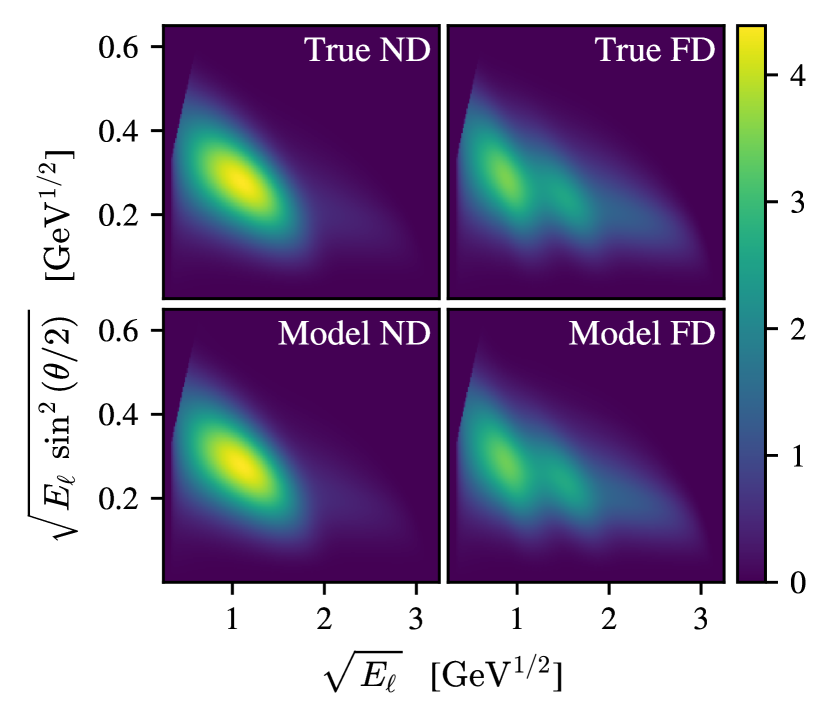
Figure 1: Event distributions at the ND (left) and FD (right) as predicted using either the True (top) or learned Model (bottom) cross sections and the true ND and FD fluxes.

The design of the training procedure is guided by the nontrivial physical requirements that the cross section be non-negative, but it decomposes into structure functions that may run negative. These cannot be simultaneously satisfied by construction of the model, and must instead be enforced by training. We therefore require a loss that is well-defined for negative values of $q_{\mathrm{ND}}$, which excludes common information-theoretic losses like the KL divergence [65]. Instead, we use the mean squared error, $\mathrm{MSE}=\displaystyle\int dE_{\ell}d\cos\theta\Bigl{[}p_{\mathrm{ND}}(E_{\ell},\cos\theta)-q_{\mathrm{ND}}(E_{\ell},\cos\theta)\Bigr{]}^{2}$. Because $p_{\mathrm{ND}}$ is non-negative, this choice drives $q_{\mathrm{ND}}$ to be non-negative without any additional regularization.

For computational expediency, we discretize all integrals on regular grids over $E_{\nu}$, $v_{1}\equiv\sqrt{E_{\ell}}$, and $v_{2}\equiv\sqrt{E_{\ell}\sin^{2}(\theta/2)}$. Changing variables $(E_{\ell},\cos\theta)\rightarrow(v_{1},v_{2})$ gives more even distribution of the ND and FD densities, as visible in Fig. 1, and thus reduces discretization errors. We note that for an at-scale application, there is no obstacle to the more principled approach of direct Monte Carlo integration over ND events, which, moreover, will obviate the need for any ND histogram construction.

This motivates our ML setup in the abstract. Concretely, the results shown are for a model with the three $W_{i}$ parametrized as the three output channels of a single multi-layer perceptron (MLP) with two input channels for $x$ and $Q^{2}$, and 4 hidden layers of width 64 with LeakyReLU activations. For training, we use a $256\times 128^{2}$ grid over $0\leq E_{\nu}\leq 10~\mathrm{GeV}$, $0.25\leq v_{1}/\mathrm{GeV}^{1/2}\leq 2.5$, and $0\leq v_{2}/\mathrm{GeV}^{1/2}\leq 0.65$. The integral defining the MSE loss is thus evaluated on a $128^{2}$ grid in $v_{1}$ and $v_{2}$. We apply $10^{4}$ steps of the Adam optimizer [66] using default hyperparameters. Note that because the loss is not evaluated stochastically, training is fully deterministic after the random initialization of the model weights.

The result is a close approximation of the true cross section, as apparent in the comparisons of Fig. 1. See the Supplemental Material for detailed comparisons of true and model structure functions and three-dimensional cross sections. Note that perfect knowledge of the entire cross section is not necessary, only of the parts relevant for far-detector kinematics. The comparison of far-detector densities indicates that this has been achieved, as can be verified by carrying out an oscillation analysis.

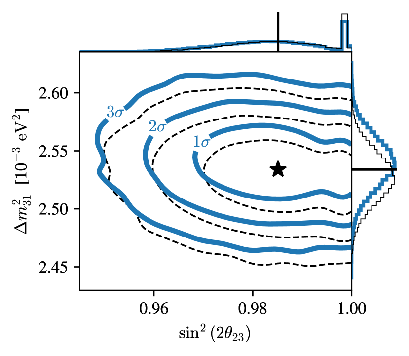
Figure 2: Confidence intervals inferred using either the true cross section (dashed black) or the learned model one (solid blue) with 6200 far-detector events, determined by bootstrapping $25000$ times through far-detector likelihood maximization. The stars and vertical lines indicate the true values. The histograms over bootstrap samples at the edges represent the marginal distributions of each inferred parameter. Contour lines are computed using a kernel density estimate (KDE) over the bootstrap samples.

Neutrino oscillation analysis — The flux of muon neutrinos reaching the far detector, $\Phi_{\mathrm{FD}}(E_{\nu})$, can be modeled by $\widetilde{\Phi}_{\mathrm{FD}}(E_{\nu};\omega)\equiv\Phi_{\rm ND}(E_{\nu})P_{\mu\mu}(E_{\nu};\omega)$, where the muon neutrino survival probability $P_{\mu\mu}$ depends on the oscillation parameters collectively denoted $\omega$. If the true cross section were known, it could be combined with $\widetilde{\Phi}_{\mathrm{FD}}$ per Eq. (5) to define a model of the FD event distribution, $\tilde{p}_{\mathrm{FD}}(E_{\ell},\cos\theta;\omega)$, which could be used to infer $\omega$. In reality, we have access only to models of the cross section that provide FD event distribution models $\tilde{q}_{\mathrm{FD}}(E_{\ell},\cos\theta;\omega)$. A successful ML model $\tilde{q}_{\mathrm{FD}}$ should provide comparable results for oscillation analyses to what would be obtained using $\tilde{p}_{\mathrm{FD}}$ with the same FD statistics.

For the sake of this exercise, we consider only $\sin^{2}(2\theta_{23})$ and $\Delta m_{31}^{2}$, with all other parameters fixed to truth. The muon disappearance channel alone does not provide good sensitivity to the octant, both in our toy model here and in DUNE projections [3]. Our analysis thus enforces normal ordering and constrains the variable $\sin^{2}(2\theta_{23})$, which is insensitive to the octant degeneracy that otherwise complicates the analysis; see the Supplemental Material. It will be essential to include electron appearance in more sophisticated analyses to constrain the octant.

We use maximum likelihood estimation (MLE) to infer the oscillation parameters $\omega$, i.e., for a sample of $N$ far-detector events $\{E_{\ell}^{(i)},\cos\theta^{(i)}\}$ distributed per $p_{\mathrm{FD}}$, we take $\mathrm{argmax}_{\omega}\,\mathcal{L}(\omega)$ where

$$\mathcal{L}(\omega)=\prod_{i=1}^{N}\tilde{p}_{\mathrm{FD}}(E_{\ell}^{(i)},\cos\theta^{(i)};\omega),$$ (6)

for the true cross section, and similarly for the model cross section with $\tilde{p}_{\mathrm{FD}}\rightarrow\tilde{q}_{\mathrm{FD}}$. During FD inference, we define the model cross section with would-be negative values ($\sim 3\%$) clamped to zero. We evaluate Eq. (6) over 6200 simulated events sampled from $p_{\mathrm{FD}}$, matching the FD statistics expected after 3.5 years of running DUNE in neutrino mode [3]. We employ bootstrap resampling [67, 68, 69] to study uncertainty by generating $25000$ synthetic datasets, each by drawing 6200 samples with replacement from the original, and computing the MLE estimate in each.

Figure 2 shows confidence intervals constructed from the resulting bootstrapped estimates of $\sin^{2}(2\theta_{23})$ and $\Delta m^{2}_{31}$. Using the cross-section model provides a nearly identical estimate as to what would be obtained if the cross section were known exactly—recall that the plot represents only a small patch of the allowed values. Although the modeling induces a clear deviation from truth, the model predictions are consistent with the true value well within $1\sigma$. True and model confidence intervals are of similar shape and extent, indicating good estimation of uncertainties with no artificial reduction due to mismodeling. The octant degeneracy in $\sin\theta_{23}$ is largely mitigated by studying $\sin^{2}(2\theta_{23})$; however, the tall bin at the right of the $\sin^{2}(2\theta_{23})$ histogram in Fig. 2 can be attributed to this degeneracy as discussed in the Supplemental Material. We note that these sensitivities do not include any systematic error quantification and thus should not be directly compared with DUNE projections. Nevertheless, they are drastically reduced versus DUNE, as our approach does not yet incorporate the wealth of hadronic information offered by the experiment.

Discussion — We conclude that the method passes the closure test: oscillation parameters may be inferred nearly as reliably using a model of the neutrino-nucleus cross section based on structure functions learned from data as if the true cross section were known exactly. The results of this exercise indicate that a fully data-driven analysis of long-baseline neutrino experiment data is possible, independent of and (as emphasized above) complementary to present approaches based on event generators. Our results suggest several critical topics for future work besides those already noted.

Paramount among these is rigorous and reliable uncertainty quantification. In this work, we do not attempt to systematically quantify uncertainties due to aspects of the ML setup including weights initialization and architecture and training hyperparameters. While straightforward enumeration can establish some sense of variability, how to use the resulting information to construct statistically meaningful uncertainty estimates is a challenging open question. Formally, the proposed method is a machine-learned approach to solving an inverse problem, for which uncertainty quantification is an active topic of research across the sciences [70]. Better understanding of these issues and more detailed mathematical study of the particular inverse problem treated here are critical if this approach is to be employed to study nature. In addition, experimental effects such as energy and angular smearing, finite ND statistics, and flux uncertainties must be included.

It is similarly critical to extend the data-driven approach to incorporate multiple different sources of physics information. Exclusive final-state data will be necessary to fully exploit the unprecedented resolution of the DUNE experiment, which will require a ML approach agnostic to particle multiplicity. Furthermore, as discussed above, incorporation of electron data is expected to resolve the octant degeneracy [3]. It will moreover resolve the degeneracies between the five structure functions in Eq. (1), potentially allowing a better extraction of these quantities as physics targets in their own right. The situation is more complicated for simultaneously analyzing neutrino and antineutrino data, which involve distinct structure functions for non-isoscalar nuclei such as argon; further data and/or theory inputs are required. It may also be useful to incorporate data from multiple experiments with different kinematic coverage and physics priors from e.g. perturbative QCD and nuclear effective field theories. There are clear opportunities for synergy with the closely related NNSF$\nu$ approach [36], efforts to constrain NN models of response functions with electron scattering data [37], and experiments probing nuclear structure such as the Electron-Ion Collider (EIC) [71, 72, 73].

DUNE and other accelerator neutrino experiments can provide a wealth of data enabling novel searches in the neutrino sector and new understanding of nonperturbative QCD in neutrino-nucleus scattering. Data-driven cross-section modeling with ML enables accurate neutrino oscillation analyses without any of the nuclear theory assumptions entering standard, microscopic-theory-driven approaches. Strong complementarity between data-driven and microscopic-theory-driven modeling will enable important cross checks on both approaches, e.g., tests for whether beyond-Standard-Model physics is being absorbed into data-driven cross-section models. A combination of data-driven and microscopic-theory-driven approaches provides a promising route towards maximizing the discovery potential of DUNE.

Acknowledgments: We thank Minerba Betancourt, Arie Bodek, Steven Gardner, Alessandro Lovato, Pedro Machado, Luke Pickering, and Noemi Rocco for useful discussions. This manuscript has been authored by Fermi Research Alliance, LLC under Contract No. DE-AC02-07CH11359 with the U.S. Department of Energy, Office of Science, Office of High Energy Physics. The work of J.I. was supported by the U.S. Department of Energy, Office of Science, Office of Advanced Scientific Computing Research, Scientific Discovery through Advanced Computing (SciDAC-5) program, grant “NeuCol”. The work of K.T. is supported by DOE Grant KA2401045. Numerical experiments and data analysis were performed using PyTorch [74], NumPy [75], SciPy [76], pandas [77, 78], gvar [79], Mathematica [80], and LHAPDF6 [59]. Figures were produced using matplotlib [81].

Supplemental Material

This Supplemental Material provides additional details on several topics complementing the main text: the ML optimization (training) procedure, a comparison of the three-dimensional true and model cross sections, the structure function extraction, and the octant degeneracy in the oscillation analysis.

Appendix A Additional ML details

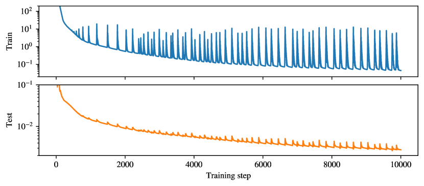
Figure A1: History of training loss (MSE, as defined in the main text) and test loss (as discussed in the text) over the full course of training the model used to produce the results of the main text. Note that large values at early training times are outside the range of the plot.

Model construction and training follows the procedure defined in the main text. Training for 10000 steps takes approximately 14 minutes on an NVIDIA A100 GPU on Google Colab.

We note that there is no stochasticity in the training process. Once the initial model weights are drawn randomly, training is fully deterministic. This is because stochastic gradient descent is only stochastic when the loss (or more precisely, the gradients of the loss) are estimated stochastically. This is not the case in the method explored in this work: the integrals defining the MSE loss are computed by discretizing them on a grid, rather than using a Monte Carlo estimator or random minibatching (i.e., taking random subsets of a finite training data set).

Figure A1 shows training and test loss curves. The training loss is the MSE as defined in the main text; the test loss is defined below. The structure in the training loss curve—smooth descent interrupted by large spikes, then a decay back to the previous value—reflects an instability in the training process. In the authors’ experience, such instabilities often arise when training neural networks using non-stochastic losses. This instability is not a practical problem. Considering the lower envelope of the loss curve, it is clear that the quality of optimization continues to increase over time on the whole, with only transient disruptions. To avoid finding a bad model if training concludes in the midst of such an event, we retain a copy of the model for the best loss observed thus far, and take that as the final output of training. For the model used in the main text, this occurs on the 9996th training step out of 10000.

Note that the ND and FD inference problems are each defined in terms of marginal distributions, i.e. $p_{\mathrm{ND}}$, $q_{\mathrm{ND}}$, $\tilde{p}_{\mathrm{FD}}$, and $\tilde{q}_{\mathrm{FD}}$. Computing a properly normalized marginal from a cross section and flux per Eq. (5) requires divison by $\int dE_{\nu}dE_{\ell}\cos\theta\,\frac{d^{2}\sigma}{dE_{\ell}d\cos\theta}\phi$. This means that the marginal distributions are each invariant under overall rescalings of the flux or cross section. Consequently, none of the inference problems considered here—neither learning the cross section at the ND nor the oscillation analysis at the FD—are sensitive to the overall scale of the flux or cross section. Thus, the model cross section and structure functions can only expected to be correct up to an overall scale factor, even in the limit of perfect modeling.

This overall scale factor may be negative. That this can occur does not pose any practical issue, because it can always be identified by examining the model cross section, which should be positive everywhere. In fact, the final model used in the main text as initially trained is off by an overall sign, parameterizing a cross section which is negative (almost) everywhere. With no loss of rigor, we redefine the model after training as the outputs of the original function multiplied by $-1$. We emphasize that the inference problems are insensitive to this sign regardless, but it will be important if structure functions are a desired output.

While not possible when modeling an unknown cross section, in the toy-model setting, we know the true three-dimensional cross section and thus are able to compare it to the model one. The test loss shown in Fig. A1 encodes this comparison. Because the cross section can be learned only up to an overall scale, this comparison requires first defining normalized quantities. In particular, we compute

$$S_{p}(E_{\nu},E_{\ell},\cos\theta)\equiv\frac{\frac{d^{2}\sigma}{dE_{\ell}d\cos\theta}(E_{\nu})}{\int dE_{\nu}dE_{\ell}d\cos\theta~\frac{d^{2}\sigma}{dE_{\ell}d\cos\theta}(E_{\nu})}~,$$ (7)

and similarly $S_{q}$ from the model cross section, from which the test loss is defined as

$$\int dE_{\nu}dE_{\ell}\,d\cos\theta\,\left|S_{p}-S_{q}\right|^{2}~.$$ (8)

Note that these are written in terms of $E_{\ell},\cos\theta$ to avoid confusion, but in practice, we compute these integrals discretized over $v_{1}=\sqrt{E_{\ell}}$ and $v_{2}=\sqrt{E_{\ell}\sin^{2}(\theta/2)}$ kinematics as discussed in the main text.

The behavior of the test loss in Fig. A1 implies that training smoothly produces an increasingly high-quality approximation of the cross section across its full kinematic range in all three dimensions. This is despite the fact that training only has access to $p_{\mathrm{ND}}$, a two-dimensional marginalization of the full three-dimensional object. Interestingly, while some sign of the same instabilities observed in the train loss are visible in the test loss, the overall size of the effect is much reduced. It may be interesting to determine the dynamics underlying this difference.

Appendix B Cross-section comparison

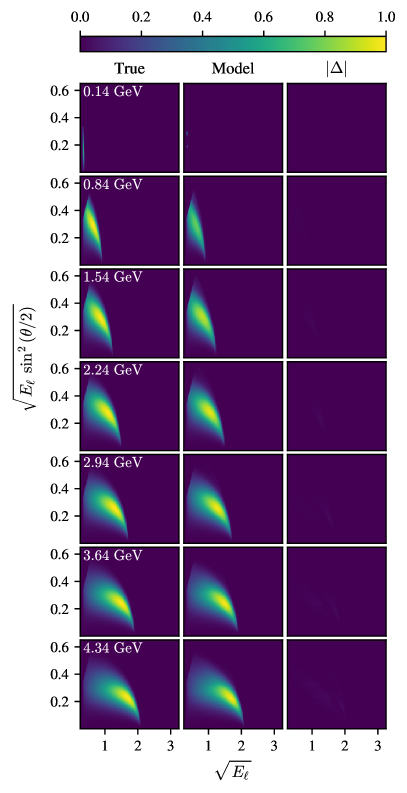
Figure A2: Comparisons of true and model cross sections along slices of fixed $E_{\nu}$ interpolating the full range of $0\leq E_{\nu}\leq 10~\mathrm{GeV}$. Each cross section is first normalized as described in the text to remove an overall scale, then within each row the maximum value over either true or model is divided out of both. Not visible given this normalization convention is that $\frac{d^{2}\sigma}{dv_{1}dv_{2}}$ increases as a function of $E_{\nu}$, as shown in Fig. A3.

Figure A2 compares the true and model cross sections, evaluated on slices of fixed $E_{\nu}$ and shown for $(v_{1},v_{2})$ kinematics. At lower $E_{\nu}$, differences $|\Delta|$ between model and true are difficult to see when rendered with the same colormap as the cross section. Close inspection at high $E_{\nu}$ reveals some small but clearly structured differences.

Considering the total cross section $\sigma(E_{\nu})=\int dE_{\ell}d\cos\theta\,\frac{d^{2}\sigma}{dE_{\ell}d\cos\theta}(E_{\nu})$ allows the size of these $E_{\nu}$-dependent discrepancies to be quantified. To remove the overall scale ambiguity, we consider the normalized cross section $\sigma(E_{\nu})/\int dE_{\nu}\sigma(E_{\nu})$, where the integral is evaluated over the full kinematic range $0\leq E_{\nu}\leq 10~\mathrm{GeV}$ of the toy model. Note that this definition amounts to simply integrating over the slices shown in Fig. A2 and normalizing. Figure A3 compares this quantity as computed using the true and model cross sections, confirming good agreement over most of the kinematic range, with deviations increasing at high $E_{\nu}$.

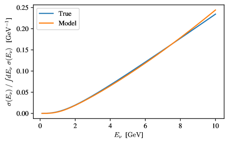
Figure A3: Comparison of true and model normalized (total) cross sections.

Appendix C Structure functions

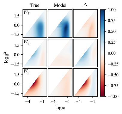
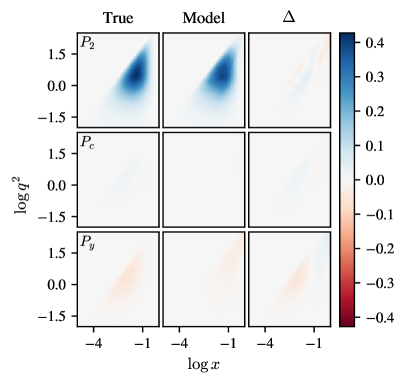
Figure A4: Comparison of true and model structure functions without (left) and with (right) weights accounting for which kinematic regions are well-constrained by the available ND data. The masked regions are fully unconstrained due to $E_{\nu}\leq 10~\mathrm{GeV}$. For each set of true and model structure functions separately, the overall scale of the $W_{i}$ is set by dividing the overall maximum. The relative scales between different structure functions are thus left intact and encoded in the colormaps.

As demonstrated, the cross section can be learned accurately over relevant kinematic ranges using ND data. Ideally, the nuclear structure functions $W_{i}$ would also be a well-estimated physics output of the analysis. In practice, however, they are not as obviously well-modeled as the cross section, as apparent from the left panel of Fig. A4. Furthermore, the unclear relation between true and model $W_{i}$ naively seems inconsistent with the high quality of approximation of the cross section.

The source of this apparent discrepancy is that the ND marginal $p_{\mathrm{ND}}$ is related to the structure functions with nontrivially $(x,Q^{2})$-dependent weights by the combination of the ND flux $\Phi_{\mathrm{ND}}$ and the kinematic factors of Eq. (2). Via these weights, the ND data constrain only a small range of all $(x,Q^{2})$, outside of which the model is free to vary without significantly affecting $q_{\mathrm{ND}}\approx p_{\mathrm{ND}}$ (and, critically, $q_{\mathrm{FD}}\approx p_{\mathrm{FD}}$). For example, the whited-out regions in Fig. A4 are those for which there are no constraints at all, due to the maximum $E_{\nu}=10$ defined for the toy model.

Accounting for this kinematic weighting paints a clearer picture. Because $p_{\mathrm{ND}}(E_{\ell},\cos\theta)$ is obtained by marginalizing over $E_{\nu}$, it is nontrivially related to $W_{i}(x,Q^{2})$, with any given point in $(E_{\ell},\cos\theta)$ in principle constraining the $W_{i}$ over the full range of $(x,Q^{2})$. While it may be interesting to explore applications of the four-dimensional weight function that this defines, a simpler option is available in the toy model setting: we may instead consider the three-dimensional ND event distribution $\mathcal{P}_{\mathrm{ND}}$ in $(x,y,Q^{2})$ kinematics, and marginalize over $y$. First, note that $\mathcal{P}_{\mathrm{ND}}$ may be decomposed into a contribution from each structure function:

$$\mathcal{P}_{\mathrm{ND}}(x,y,Q^{2})\equiv\frac{1}{\mathcal{N}}\Phi_{\mathrm{ND}}(E_{\nu}(x,y,Q^{2}))~\frac{d^{2}\sigma}{dxdy}(Q^{2}) =\frac{1}{\mathcal{N}}\Phi_{\mathrm{ND}}(E_{\nu}(x,y,Q^{2}))~\sum_{i}K_{i}(x,y,Q^{2})W_{i}(x,Q^{2})$$ (9)

$$=\sum_{i}\left[\frac{1}{\mathcal{N}}\Phi_{\mathrm{ND}}(E_{\nu}(x,y,Q^{2}))~K_{i}(x,y,Q^{2})\right]W_{i}(x,Q^{2})$$

where $K_{i}$ are the kinematic coefficients of the structure functions from Eq. (2) and

$$\mathcal{N}\equiv\int dxdydQ^{2}~\frac{d^{2}\sigma}{dxdy}(Q^{2})~\Phi_{\mathrm{ND}}(E_{\nu}(x,y,Q^{2})).$$ (10)

Because $P_{\mathrm{ND}}$ is already normalized, marginalization over $y$ may be accomplished simply by integration, which allows further defining

$$\int dy~\mathcal{P}_{\mathrm{ND}}(x,y,Q^{2})\equiv\sum_{i}\mathcal{K}_{i}(x,Q^{2})W_{i}(x,Q^{2})\equiv\sum_{i}P_{i}(x,Q^{2})~.$$ (11)

The $y$-marginalized coefficient functions

$$\mathcal{K}_{i}(x,Q^{2})\equiv\int dy\frac{1}{\mathcal{N}}\Phi_{\mathrm{ND}}(E_{\nu}(x,y,Q^{2}))~K_{i}(x,y,Q^{2})$$ (12)

define $(x,Q^{2})$-dependent weights which encode exactly which regions of the $W_{i}$ are relevant to ND kinematics. Multiplying them on to $W_{i}$ defines $P_{i}(x,Q^{2})$, which are the contributions associated with each $W_{i}$ to the total marginal $P(x,Q^{2})\equiv\int dy~\mathcal{P}(x,y,Q^{2})$, such that $\sum_{i}P_{i}=P$.

The right panel of Fig. A4 compares the true and model structure functions with these kinematic weights applied to obtain $P_{i}(x,Q^{2})$. It is clear that $W_{2}$ is the overwhelming contribution, with $W_{2}$ and $W_{y}$ heavily kinematically suppressed. This furthermore makes apparent that the kinematically relevant part of $W_{2}$ is well-modeled, explaining the high-quality approximation of the cross section. More substantial mismodeling of $W_{y}$ and $W_{c}$ is faintly visible, but the overall scale of these effects are clearly subleading.

This analysis indicates that further refinements will be required if the structure functions themselves are the objects of interest, except for $W_{2}$ in a particular kinematic region. While it may be possible to improve the extraction with additional methods developments, incorporating additional physics information provides a clear path to improvement. For example, adding electron information allows in principle separately constraining all five $W_{i}$ of Eq. (1). Furthermore, an approach similar to that of NNSF$\nu$ [36], which fits SFs to multiple experiments with different systematic effects, would enable stronger constraints on different kinematical regions. However, many experiments use different targets; incorporating these data together requires some modeling of the dependence of the SFs on the proton and neutron number, and thus additional nuclear theory inputs.

Appendix D Oscillation analysis

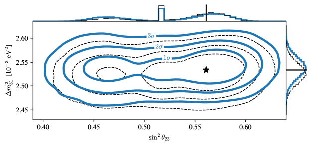
Figure A5: Confidence intervals as in Fig. 2, but in the $\sin^{2}\theta_{23}-\Delta m^{2}_{31}$ plane. Dashed black lines indicate results obtained using the true cross section and solid blue lines results obtained with the learned model one, determined by bootstrapping $25000$ times through far-detector likelihood maximization. The stars and vertical lines indicate the true values. The histograms over bootstrap samples at the edges represent the marginal distributions of each inferred parameter. Contour lines are computed using a kernel density estimate (KDE) over the bootstrap samples.

As discussed in the main text, the muon disappearance channel does not provide good octant sensitivity with the available statistics, even using the true cross section. In particular, this arises as two near-degenerate minima in $\sin^{2}\theta_{23}$ which are difficult to resolve without high statistics. In the main analysis, we worked around this issue by instead constraining the variable $\sin^{2}(2\theta_{23})$ which is insensitive to the octant by construction. For comparison, Figure A5 presents the oscillation analysis for $\sin^{2}\theta_{23}$ instead. The confidence intervals show clear bimodality, with little preference for either mode. The unusually tall bin in the marginal histogram in $\sin^{2}\theta_{23}$ indicates that in a large fraction of bootstraps, the two minima are not resolved from one another (i.e., single-welled vs. double-welled) such that MLE finds an intermediate value. We note, however, that the quality of the model cross section is similarly apparent as in Fig. 2.

References

- An et al. [2016] F. An et al. (JUNO), J. Phys. G 43, 030401 (2016), arXiv:1507.05613 [physics.ins-det] .
- Abe et al. [2018] K. Abe et al. (Hyper-Kamiokande), (2018), arXiv:1805.04163 [physics.ins-det] .
- Abi et al. [2020] B. Abi et al. (DUNE), (2020), arXiv:2002.03005 [hep-ex] .
- Alvarez-Ruso et al. [2018] L. Alvarez-Ruso et al. (NuSTEC), Prog. Part. Nucl. Phys. 100, 1 (2018), arXiv:1706.03621 [hep-ph] .
- Ruso et al. [2022] L. A. Ruso et al., (2022), arXiv:2203.09030 [hep-ph] .
- de Gouvêa et al. [2022] A. de Gouvêa et al., (2022), arXiv:2209.07983 [hep-ph] .
- Ankowski et al. [2015a] A. M. Ankowski, O. Benhar, P. Coloma, P. Huber, C.-M. Jen, C. Mariani, D. Meloni, and E. Vagnoni, Phys. Rev. D 92, 073014 (2015a), arXiv:1507.08560 [hep-ph] .
- Khachatryan et al. [2021] M. Khachatryan et al. (CLAS, e4v), Nature 599, 565 (2021).
- Acero et al. [2022] M. A. Acero et al. (NOvA), Phys. Rev. D 106, 032004 (2022), arXiv:2108.08219 [hep-ex] .
- Abe et al. [2021] K. Abe et al. (T2K), Phys. Rev. D 103, 112008 (2021), arXiv:2101.03779 [hep-ex] .
- Abe et al. [2023] K. Abe et al. (T2K), Eur. Phys. J. C 83, 782 (2023), arXiv:2303.03222 [hep-ex] .
- Ankowski et al. [2015b] A. M. Ankowski, P. Coloma, P. Huber, C. Mariani, and E. Vagnoni, Phys. Rev. D 92, 091301 (2015b), arXiv:1507.08561 [hep-ph] .
- Friedland and Li [2019] A. Friedland and S. W. Li, Phys. Rev. D 99, 036009 (2019), arXiv:1811.06159 [hep-ph] .
- Friedland and Li [2020] A. Friedland and S. W. Li, Phys. Rev. D 102, 096005 (2020), arXiv:2007.13336 [hep-ph] .
- Abratenko et al. [2022] P. Abratenko et al. (MicroBooNE), Phys. Rev. Lett. 128, 241801 (2022), arXiv:2110.14054 [hep-ex] .
- Abratenko et al. [2024a] P. Abratenko et al. (MicroBooNE), Eur. Phys. J. C 84, 1052 (2024a), arXiv:2406.10583 [hep-ex] .
- Andreopoulos et al. [2010] C. Andreopoulos et al., Nucl. Instrum. Meth. A 614, 87 (2010), arXiv:0905.2517 [hep-ph] .
- Buss et al. [2012] O. Buss, T. Gaitanos, K. Gallmeister, H. van Hees, M. Kaskulov, O. Lalakulich, A. B. Larionov, T. Leitner, J. Weil, and U. Mosel, Phys. Rept. 512, 1 (2012), arXiv:1106.1344 [hep-ph] .
- Golan et al. [2012] T. Golan, J. T. Sobczyk, and J. Zmuda, Nucl. Phys. B Proc. Suppl. 229-232, 499 (2012).
- Aliaga et al. [2014] L. Aliaga et al. (MINERvA), Nucl. Instrum. Meth. A 743, 130 (2014), arXiv:1305.5199 [physics.ins-det] .
- Hayato and Pickering [2021] Y. Hayato and L. Pickering, Eur. Phys. J. ST 230, 4469 (2021), arXiv:2106.15809 [hep-ph] .
- Isaacson et al. [2023] J. Isaacson, W. I. Jay, A. Lovato, P. A. N. Machado, and N. Rocco, Phys. Rev. D 107, 033007 (2023), arXiv:2205.06378 [hep-ph] .
- Abratenko et al. [2024b] P. Abratenko et al. (MicroBooNE), Phys. Rev. Lett. 133, 041801 (2024b), arXiv:2402.19281 [hep-ex] .
- Beane et al. [2000] S. R. Beane, P. F. Bedaque, W. C. Haxton, D. R. Phillips, and M. J. Savage 10.1142/9789812810458_0011 (2000), arXiv:nucl-th/0008064 .
- Epelbaum et al. [2009] E. Epelbaum, H.-W. Hammer, and U.-G. Meissner, Rev. Mod. Phys. 81, 1773 (2009), arXiv:0811.1338 [nucl-th] .
- Kaplan [2020] D. B. Kaplan, Phys. Rev. C 102, 034004 (2020), arXiv:1905.07485 [nucl-th] .
- Hammer et al. [2020] H. W. Hammer, S. König, and U. van Kolck, Rev. Mod. Phys. 92, 025004 (2020), arXiv:1906.12122 [nucl-th] .
- van Kolck [2020] U. van Kolck, Front. in Phys. 8, 79 (2020), arXiv:2003.06721 [nucl-th] .
- Epelbaum et al. [2022] E. Epelbaum, H. Krebs, and P. Reinert, Semi-local Nuclear Forces From Chiral EFT: State-of-the-Art and Challenges, in Handbook of Nuclear Physics, edited by I. Tanihata, H. Toki, and T. Kajino (2022) pp. 1–25, arXiv:2206.07072 [nucl-th] .
- Acero et al. [2020] M. A. Acero et al. (NOvA), Eur. Phys. J. C 80, 1119 (2020), arXiv:2006.08727 [hep-ex] .
- Stowell et al. [2019] P. Stowell et al. (MINERvA), Phys. Rev. D 100, 072005 (2019), arXiv:1903.01558 [hep-ex] .
- Coyle et al. [2022] N. M. Coyle, S. W. Li, and P. A. N. Machado, JHEP 12, 166, arXiv:2210.03753 [hep-ph] .
- Ball et al. [2012] R. D. Ball, V. Bertone, F. Cerutti, L. Del Debbio, S. Forte, A. Guffanti, J. I. Latorre, J. Rojo, and M. Ubiali (NNPDF), Nucl. Phys. B 855, 153 (2012), arXiv:1107.2652 [hep-ph] .
- Abdul Khalek et al. [2019] R. Abdul Khalek, J. J. Ethier, and J. Rojo (NNPDF), Eur. Phys. J. C 79, 471 (2019), arXiv:1904.00018 [hep-ph] .
- Forte et al. [2002] S. Forte, L. Garrido, J. I. Latorre, and A. Piccione, JHEP 05, 062, arXiv:hep-ph/0204232 .
- Candido et al. [2023] A. Candido, A. Garcia, G. Magni, T. Rabemananjara, J. Rojo, and R. Stegeman, JHEP 05, 149, arXiv:2302.08527 [hep-ph] .
- Sobczyk et al. [2024] J. E. Sobczyk, N. Rocco, and A. Lovato, Phys. Lett. B 859, 139142 (2024), arXiv:2406.06292 [nucl-th] .
- Abe et al. [2017] K. Abe et al. (T2K), Phys. Rev. D 95, 111101 (2017), arXiv:1703.01361 [hep-ex] .
- Machado et al. [2019] P. A. Machado, O. Palamara, and D. W. Schmitz, Ann. Rev. Nucl. Part. Sci. 69, 363 (2019), arXiv:1903.04608 [hep-ex] .
- Altmannshofer et al. [2019] W. Altmannshofer, S. Gori, J. Martín-Albo, A. Sousa, and M. Wallbank, Phys. Rev. D 100, 115029 (2019), arXiv:1902.06765 [hep-ph] .
- de Gouvea et al. [2020] A. de Gouvea, P. A. N. Machado, Y. F. Perez-Gonzalez, and Z. Tabrizi, Phys. Rev. Lett. 125, 051803 (2020), arXiv:1912.06658 [hep-ph] .
- Berryman et al. [2020] J. M. Berryman, A. de Gouvea, P. J. Fox, B. J. Kayser, K. J. Kelly, and J. L. Raaf, JHEP 02, 174, arXiv:1912.07622 [hep-ph] .
- Ellis et al. [2020a] S. A. R. Ellis, K. J. Kelly, and S. W. Li, Phys. Rev. D 102, 115027 (2020a), arXiv:2004.13719 [hep-ph] .
- Ellis et al. [2020b] S. A. R. Ellis, K. J. Kelly, and S. W. Li, JHEP 12, 068, arXiv:2008.01088 [hep-ph] .
- Acero et al. [2021] M. A. Acero et al. (NOvA), Phys. Rev. Lett. 127, 201801 (2021), arXiv:2106.04673 [hep-ex] .
- Acciarri et al. [2023] R. Acciarri et al. (ArgoNeuT), Phys. Rev. Lett. 130, 221802 (2023), arXiv:2207.08448 [hep-ex] .
- Abratenko et al. [2024c] P. Abratenko et al. (MicroBooNE), Phys. Rev. Lett. 132, 041801 (2024c), arXiv:2310.07660 [hep-ex] .
- Abratenko et al. [2024d] P. Abratenko et al. (MicroBooNE), Phys. Rev. Lett. 132, 241801 (2024d), arXiv:2312.13945 [hep-ex] .
- Coloma et al. [2024] P. Coloma, J. Martín-Albo, and S. Urrea, Phys. Rev. D 109, 035013 (2024), arXiv:2309.06492 [hep-ph] .
- Albright and Jarlskog [1975] C. H. Albright and C. Jarlskog, Nucl. Phys. B 84, 467 (1975).
- Paschos and Yu [2002] E. A. Paschos and J. Y. Yu, Phys. Rev. D 65, 033002 (2002), arXiv:hep-ph/0107261 .
- Kretzer and Reno [2002] S. Kretzer and M. H. Reno, Phys. Rev. D 66, 113007 (2002), arXiv:hep-ph/0208187 .
- Tomalak et al. [2022a] O. Tomalak, Q. Chen, R. J. Hill, and K. S. McFarland, Nature Commun. 13, 5286 (2022a), arXiv:2105.07939 [hep-ph] .
- Tomalak et al. [2022b] O. Tomalak, Q. Chen, R. J. Hill, K. S. McFarland, and C. Wret, Phys. Rev. D 106, 093006 (2022b), arXiv:2204.11379 [hep-ph] .
- Afanasev et al. [2024] A. Afanasev et al., Eur. Phys. J. A 60, 91 (2024), arXiv:2306.14578 [hep-ph] .
- Bjorken and Paschos [1969] J. D. Bjorken and E. A. Paschos, Phys. Rev. 185, 1975 (1969).
- Callan and Gross [1969] C. G. Callan, Jr. and D. J. Gross, Phys. Rev. Lett. 22, 156 (1969).
- Hou et al. [2021] T.-J. Hou et al., Phys. Rev. D 103, 014013 (2021), arXiv:1912.10053 [hep-ph] .
- Buckley et al. [2015] A. Buckley, J. Ferrando, S. Lloyd, K. Nordström, B. Page, M. Rüfenacht, M. Schönherr, and G. Watt, Eur. Phys. J. C 75, 132 (2015), arXiv:1412.7420 [hep-ph] .
- Martin et al. [2009] A. D. Martin, W. J. Stirling, R. S. Thorne, and G. Watt, Eur. Phys. J. C 63, 189 (2009), arXiv:0901.0002 [hep-ph] .
- Ruiz et al. [2024] R. Ruiz et al., Prog. Part. Nucl. Phys. 136, 104096 (2024), arXiv:2301.07715 [hep-ph] .
- [62] L. Fields, DUNE Fluxes, https://glaucus.crc.nd.edu/DUNEFluxes/.
- Esteban et al. [2024] I. Esteban, M. C. Gonzalez-Garcia, M. Maltoni, I. Martinez-Soler, J. a. P. Pinheiro, and T. Schwetz, (2024), arXiv:2410.05380 [hep-ph] .
- Denton and Parke [2024] P. B. Denton and S. J. Parke, Phys. Rev. D 110, 073005 (2024), arXiv:2405.02400 [hep-ph] .
- Kullback and Leibler [1951] S. Kullback and R. A. Leibler, The Annals of Mathematical Statistics 22, 79 (1951).
- Kingma and Ba [2014] D. P. Kingma and J. Ba (2014) arXiv:1412.6980 [cs.LG] .
- Efron [1982] B. Efron, The Jackknife, the bootstrap and other resampling plans, Regional Conference Series in applied mathematics No. 38 (Society for Industrial and Applied Mathematics, Philadelphia, Pa., 1982).
- DiCiccio and Efron [1996] T. J. DiCiccio and B. Efron, Statistical Science 11, 189 (1996).
- Davison and Hinkley [1997] A. C. Davison and D. V. Hinkley, The basic bootstraps, in Bootstrap Methods and their Application, Cambridge Series in Statistical and Probabilistic Mathematics (Cambridge University Press, 1997) p. 11–69.
- He et al. [2024] W. He, Z. Jiang, T. Xiao, Z. Xu, and Y. Li, (2024), arXiv:2302.13425 [cs.LG] .
- Accardi et al. [2016] A. Accardi et al., Eur. Phys. J. A 52, 268 (2016), arXiv:1212.1701 [nucl-ex] .
- Abdul Khalek et al. [2022a] R. Abdul Khalek et al., Nucl. Phys. A 1026, 122447 (2022a), arXiv:2103.05419 [physics.ins-det] .
- Abdul Khalek et al. [2022b] R. Abdul Khalek et al., (2022b), arXiv:2203.13199 [hep-ph] .
- Paszke et al. [2019] A. Paszke et al., in Advances in Neural Information Processing Systems 32, edited by H. Wallach, H. Larochelle, A. Beygelzimer, F. d'Alché-Buc, E. Fox, and R. Garnett (Curran Associates, Inc., 2019) pp. 8024–8035.
- Harris et al. [2020] C. R. Harris, K. J. Millman, S. J. van der Walt, R. Gommers, P. Virtanen, D. Cournapeau, E. Wieser, J. Taylor, S. Berg, N. J. Smith, R. Kern, M. Picus, S. Hoyer, M. H. van Kerkwijk, M. Brett, A. Haldane, J. F. del Río, M. Wiebe, P. Peterson, P. Gérard-Marchant, K. Sheppard, T. Reddy, W. Weckesser, H. Abbasi, C. Gohlke, and T. E. Oliphant, Nature 585, 357 (2020).
- Virtanen et al. [2020] P. Virtanen, R. Gommers, T. E. Oliphant, M. Haberland, T. Reddy, D. Cournapeau, E. Burovski, P. Peterson, W. Weckesser, J. Bright, S. J. van der Walt, M. Brett, J. Wilson, K. J. Millman, N. Mayorov, A. R. J. Nelson, E. Jones, R. Kern, E. Larson, C. J. Carey, İ. Polat, Y. Feng, E. W. Moore, J. VanderPlas, D. Laxalde, J. Perktold, R. Cimrman, I. Henriksen, E. A. Quintero, C. R. Harris, A. M. Archibald, A. H. Ribeiro, F. Pedregosa, P. van Mulbregt, and SciPy 1.0 Contributors, Nature Methods 17, 261 (2020).
- Reback et al. [2020] J. Reback, W. McKinney, jbrockmendel, J. V. den Bossche, T. Augspurger, P. Cloud, gfyoung, Sinhrks, A. Klein, M. Roeschke, S. Hawkins, J. Tratner, C. She, W. Ayd, T. Petersen, M. Garcia, J. Schendel, A. Hayden, MomIsBestFriend, V. Jancauskas, P. Battiston, S. Seabold, chris b1, h vetinari, S. Hoyer, W. Overmeire, alimcmaster1, K. Dong, C. Whelan, and M. Mehyar, pandas-dev/pandas: Pandas 1.0.3 (2020).
- Wes McKinney [2010] Wes McKinney, in Proceedings of the 9th Python in Science Conference, edited by Stéfan van der Walt and Jarrod Millman (2010) pp. 56 – 61.
- Lepage [2020] G. P. Lepage doi:10.5281/zenodo.4290884 (2020), https://github.com/gplepage/gvar .
- [80] Wolfram Research Inc., Mathematica, Version 14.0, https://www.wolfram.com/mathematica.
- Hunter [2007] J. D. Hunter, Computing in Science & Engineering 9, 90 (2007).