longtable mm[#1]

PyBOP: A Python package for battery model optimisation and parameterisation

Summary

The Python Battery Optimisation and Parameterisation (PyBOP) package provides methods for estimating and optimising battery model parameters, offering both deterministic and stochastic approaches with example workflows to assist users. PyBOP enables parameter identification from data for various battery models, including the electrochemical and equivalent circuit models provided by the popular open-source PyBaMM package (ref-Sulzer:2021Sulzer et al., 2021). Using the same approaches, PyBOP can also be used for design optimisation under user-defined operating conditions across a variety of model structures and design goals. PyBOP facilitates optimisation with a range of methods, with diagnostics for examining optimiser performance and convergence of the cost and corresponding parameters. Identified parameters can be used for prediction, on-line estimation and control, and design optimisation, accelerating battery research and development.

Statement of need

PyBOP is a Python package providing a user-friendly, object-oriented interface for optimising battery model parameters. PyBOP leverages the open-source PyBaMM package (ref-Sulzer:2021Sulzer et al., 2021) to formulate and solve battery models. Together, these tools serve a broad audience including students, engineers, and researchers in academia and industry, enabling the use of advanced models where previously this was not possible without specialised knowledge of battery modelling, parameter inference, and software development. PyBOP emphasises clear and informative diagnostics and workflows to support users with varying levels of domain expertise, and provides access to a wide range of optimisation and sampling algorithms. These are enabled through interfaces to PINTS (ref-Clerx:2019Clerx et al., 2019), SciPy (ref-SciPy:2020Virtanen et al., 2020), and PyBOP’s own implementations of algorithms such as adaptive moment estimation with weight decay (AdamW) (ref-Loshchilov:2017Loshchilov & Hutter, 2017), gradient descent (ref-Cauchy:1847Cauchy & others, 1847), and cuckoo search (ref-Yang:2009Yang & Suash Deb, 2009).

PyBOP supports the battery parameter exchange (BPX) standard (ref-BPX:2023Korotkin et al., 2023) for sharing parameter sets. These are typically costly to obtain due to the specialised equipment and time required for characterisation experiments, the need for domain knowledge, and the computational cost of estimation. PyBOP reduces the requirements for the latter two by providing fast parameter estimation methods, standardised workflows, and parameter set interoperability (via BPX).

PyBOP complements other lithium-ion battery modelling packages built around PyBaMM, such as liionpack for battery pack simulation (ref-Tranter2022Tranter et al., 2022) and pybamm-eis for fast numerical computation of the electrochemical impedance of any battery model. Identified PyBOP parameters are easily exportable to other packages.

Architecture

PyBOP has a layered structure enabling the necessary functionality to compute forward predictions, process results, and run optimisation and sampling algorithms. The forward model is solved using the battery modelling software PyBaMM, with construction, parameterisation, and discretisation managed by PyBOP’s model interface to PyBaMM. This provides a robust object construction process with a consistent interface between forward models and optimisers. Furthermore, identifiability metrics are provided along with the estimated parameters (through Hessian approximation of the cost functions around the optimum point in frequentist workflows, and posterior distributions in Bayesian workflows).

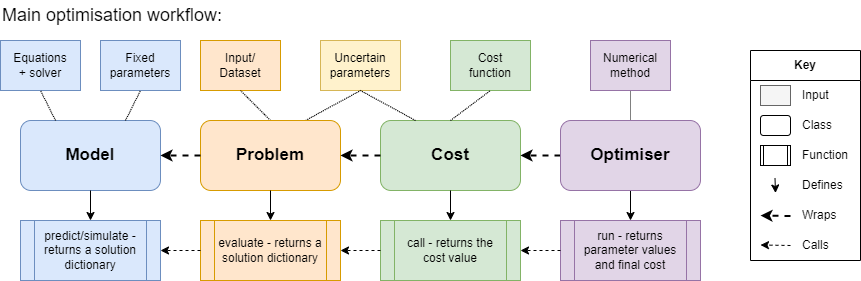
Figure 1: The core PyBOP architecture with base class interfaces. Each class provides a direct mapping to a step in the optimisation workflow.

PyBOP formulates the inference process into four key classes: model, problem, cost (or likelihood), and optimiser (or sampler), as shown in Figure 1. Each of these objects represents a base class with child classes constructing specialised functionality for different workflows. The model class constructs a PyBaMM forward model with a specified set of equations, initial conditions, spatial discretisation, and numerical solver. By composing PyBaMM directly into PyBOP, specialised models can be constructed alongside the standard models that can also be modified for different inference tasks. One such example is spatial re-discretisation, which is required when one or more geometric parameters are being optimised. In this situation, PyBOP rebuilds the PyBaMM model only when necessary, reducing the total number of rebuilds, providing improved performance. Alongside construction of the forward model, PyBOP’s model class provides methods for obtaining sensitivities from the prediction, enabling gradient-based optimisation. A forward prediction, along with its corresponding sensitivities, is provided to the problem class for processing and exception control. A standardised data structure is then provided to the cost classes, which computes a distance, design, or likelihood-based metric for optimisation. For point-based optimisation, the optimisers minimise the cost function or the negative log-likelihood if a likelihood class is provided. Bayesian inference is provided by sampler classes, which accept the LogPosterior class and sample from it using PINTS-based Monte Carlo algorithms at the time of submission. In the typical workflow, the classes in Figure 1 are constructed in sequence, from left to right in the figure.

In addition to the core architecture, PyBOP provides several specialised inference and optimisation features. One example is parameter inference from electrochemical impedance spectroscopy (EIS) simulations, where PyBOP discretises and linearises the EIS forward model into a sparse mass matrix form with accompanying auto-differentiated Jacobian. This is then translated into the frequency domain, giving a direct solution to compute the input-output impedance. In this situation, the forward models are constructed within the spatial re-discretisation workflow, allowing for geometric parameter inference from EIS simulations and data.

A second specialised feature is that PyBOP builds on the JAX (ref-jax:2018Bradbury et al., 2018) numerical solvers used by PyBaMM by providing JAX-based cost functions for automatic forward model differentiation with respect to the parameters. This functionality provides a performance improvement and allows users to harness many other JAX-based inference packages to optimise cost functions, such as NumPyro (ref-numpyro:2019Phan et al., 2019), BlackJAX (ref-blackjax:2024Cabezas et al., 2024), and Optax (ref-optax:2020DeepMind et al., 2020).

The currently implemented subclasses for the model, problem, and cost classes are listed in LABEL:tab:subclasses. The model and optimiser classes can be selected in combination with any problem-cost pair.

Table 1: List of available model, problem and cost/likelihood classes.

Battery Models	Problem Types	Cost / Likelihood
Single-particle model (SPM)	Fitting problem	Sum-squared error
SPM with electrolyte (SPMe)	Design problem	Root-mean-squared error
Doyle-Fuller-Newman (DFN)	Observer	Minkowski
Many-particle model (MPM)		Sum-of-power
Multi-species multi-reaction (MSMR)		Gaussian log likelihood
Weppner Huggins		Maximum a posteriori
Equivalent circuit model (ECM)		Volumetric energy density
		Gravimetric energy density

Similarly, the current algorithms available for optimisation are presented in LABEL:tab:subclasses. It should be noted that SciPy minimize includes several gradient and non-gradient methods. From here on, the point-based parameterisation and design-optimisation tasks will simply be referred to as optimisation tasks. This simplification can be justified by comparing Equation 5 and Equation 7; deterministic parameterisation is just an optimisation task to minimise a distance-based cost between model output and measured values.

Table 2: Currently supported optimisers classified by candidate solution type, including gradient information.

Gradient-based	Evolutionary	(Meta)heuristic
Weight decayed adaptive moment estimation (AdamW)	Covariance matrix adaptation (CMA-ES)	Particle swarm (PSO)
Improved resilient backpropagation (iRProp-)	Exponential natural (xNES)	Nelder-Mead
Gradient descent	Separable natural (sNES)	Cuckoo search
SciPy minimize	Differential evolution

In addition to deterministic optimisers LABEL:tab:subclasses, PyBOP also provides Monte Carlo sampling routines to estimate distributions of parameters within a Bayesian framework. These methods construct a posterior parameter distribution that can be used to assess uncertainty and practical identifiability. The individual sampler classes are currently composed within PyBOP from the PINTS library, with a base sampler class implemented for interoperability and direct integration with PyBOP’s model, problem, and likelihood classes. The currently supported samplers are listed in LABEL:tab:samplers.

Table 3: Sampling methods supported by PyBOP, classified according to the candidate proposal method.

Gradient-based	Adaptive	Slicing	Evolutionary	Other
Monomial gamma	Delayed rejection adaptive	Rank shrinking	Differential evolution	Metropolis random walk
No-U-turn	Haario Bardenet	Doubling		Emcee hammer
Hamiltonian	Haario	Stepout		Metropolis adjusted Langevin
Relativistic	Rao Blackwell

Background

Battery models

In general, battery models, after spatial discretisation, can be written in the form of a differential-algebraic system of equations,

$$\frac{\mathrm{d}\mathbf{x}}{\mathrm{d}t}=f(t,\mathbf{x},\boldsymbol{\theta}),$$ (1)

$$0=g(t,\mathbf{x},\boldsymbol{\theta}),$$ (2)

$$\mathbf{y}(t)=h(t,\mathbf{x},\boldsymbol{\theta}),$$ (3)

with initial conditions

$$\mathbf{x}(0)=\mathbf{x}_{0}(\boldsymbol{\theta}).$$ (4)

Here, $t$ is time, $\mathbf{x}(t)$ are the spatially discretised states, $\mathbf{y}(t)$ are the outputs (e.g. the terminal voltage) and $\boldsymbol{\theta}$ are the unknown parameters.

Common battery models include various types of equivalent circuit models (e.g. the Thévenin model), the Doyle–Fuller–Newman (DFN) model (ref-Doyle:1993Doyle et al., 1993; ref-Fuller:1994Fuller et al., 1994) based on porous electrode theory, and its reduced-order variants including the single particle model (SPM) (ref-Planella:2022Brosa Planella et al., 2022) and the multi-species multi-reaction (MSMR) model (ref-Verbrugge:2017Verbrugge et al., 2017). Simplified models that retain acceptable predictive accuracy at lower computational cost are widely used, for example in battery management systems, while physics-based models are required to understand the impact of physical parameters on performance. This separation of complexity traditionally results in multiple parameterisations for a single battery type, depending on the model structure.

Examples

Parameterisation

The parameterisation of battery models is challenging due to the large number of parameters that need to be identified compared to the number of measurable outputs (ref-Andersson:2022Andersson et al., 2022; ref-Miguel:2021Miguel et al., 2021; ref-Wang:2022Wang et al., 2022). A complete parameterisation often requires stepwise identification of smaller sets of parameters from a variety of excitations and different data sets (ref-Chen:2020Chen et al., 2020; ref-Chu:2019Chu et al., 2019; ref-Kirk:2022Kirk et al., 2023; ref-Lu:2021Lu et al., 2021). Furthermore, parameter identifiability can be poor for a given set of excitations and data sets, requiring improved experimental design in addition to uncertainty capable identification methods (ref-Aitio:2020Aitio et al., 2020).

A generic data-fitting optimisation problem may be formulated as:

$$\min_{\boldsymbol{\theta}}\leavevmode\nobreak\ \mathcal{L}_{(\hat{\mathbf{y}_{i}})}(\boldsymbol{\theta})\leavevmode\nobreak\ \leavevmode\nobreak\ \leavevmode\nobreak\ \textrm{subject to equations (\ref{dynamics}){-}(\ref{initial_conditions})}$$ (5)

where $\mathcal{L}:\boldsymbol{\theta}\mapsto[0,\infty)$ is a cost function that quantifies the agreement between the model output $\mathbf{y}(t)$ and a sequence of observations $(\hat{\mathbf{y}_{i}})$ measured at times $t_{i}$. Within the PyBOP framework, the FittingProblem class packages the model output along with the measured observations, both of which are then passed to the cost classes for the computation of the specific cost function. For gradient-based optimisers, the Jacobian of the cost function with respect to unknown parameters, $\partial\mathcal{L}/\partial\theta$, is computed for step-size and directional information.

Next, we demonstrate the fitting of synthetic data where the model parameters are known. Throughout this section, as an example, we use PyBaMM’s implementation of the single particle model with an added contact resistance submodel. We assume that the model is already fully parameterised apart from two dynamic parameters, namely, the lithium diffusivity of the negative electrode active material particles (denoted “negative particle diffusivity”) and the contact resistance with corresponding true values of [3.3e-14 $\text{m}^{2}/\text{s}$, 10 mOhm]. To start, we generate synthetic time-domain data correspondinog to a one-hour discharge from 100% to 0% state of charge, denoted as 1C rate, followed by 30 minutes of relaxation. This dataset is then corrupted with zero-mean Gaussian noise of amplitude 2 mV, with the resulting signal shown by the blue dots in Figure 2 (left). The initial states are assumed known, although this assumption is not generally necessary. The PyBOP repository contains several other example notebooks that follow a similar inference process. The underlying cost landscape to be explored by the optimiser is shown in Figure 2 (right), with the initial position denoted alongside the known true system parameters for this synthetic inference task. In general, the true parameters are not known.

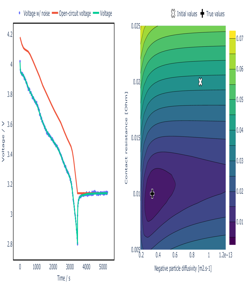
Figure 2: The synthetic fitting dataset (left) and cost landscape (right) for an example time-series battery model parameterisation using a root-mean-squared error cost function.

We can also use PyBOP’sto generate and fit electrochemical impedance data using methods within pybamm-eis that enable fast impedance computation of battery models (ref-pybamm-eisDhoot et al., 2024).Using the same model and parameters as in the time-domain case, Figure 3 shows the numerical impedance prediction available in PyBOP alongside the cost landscape for the corresponding inference task. At the time of publication, gradient-based optimisation and sampling methods are not available when using an impedance workflow.

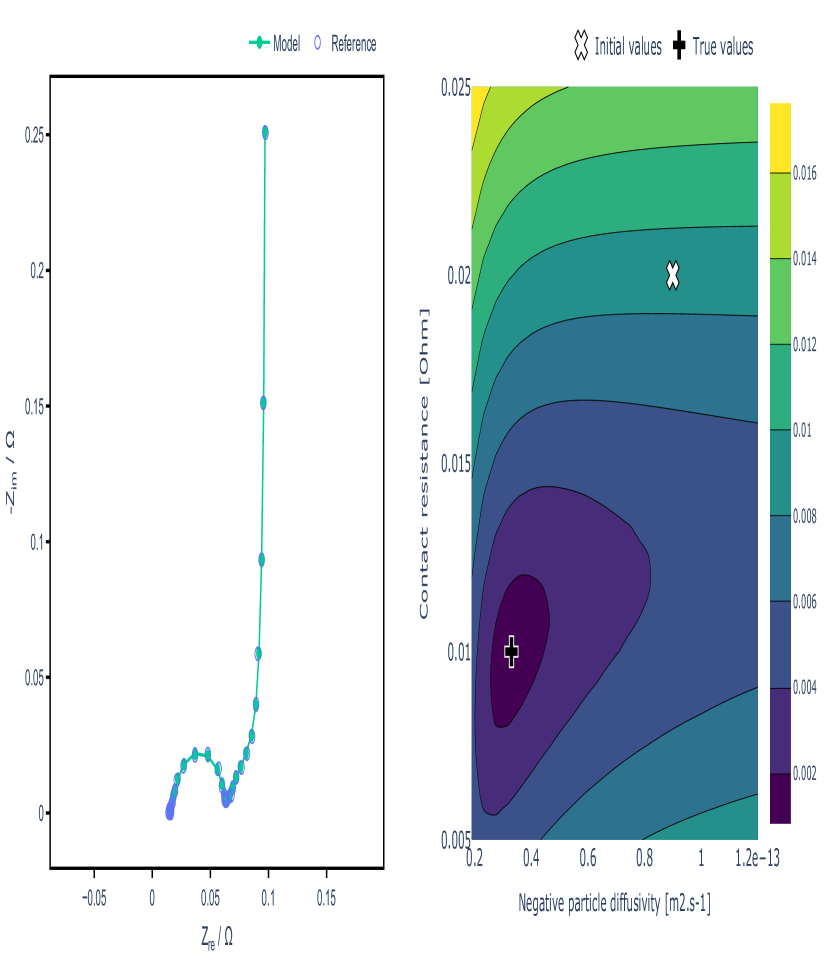
Figure 3: The data and model fit (left) and cost landscape (right) for a frequency-domain impedance parameterisation with a root-mean-squared error cost function, at 5% SOC.

To avoid confusion, we continue with identification in the time-domain (Figure 2). In general, however, time- and frequency-domain models and data may be combined for improved parameterisation. As gradient information is available for our time-domain example, the choice of distance-based cost function and optimiser is not constrained. Due to the difference in magnitude between the two parameters, we apply the logarithmic parameter transformation offered by PyBOP. This transforms the search space of the optimiser to allow for a common step size between the parameters, improving convergence in this particular case. As a demonstration of the parameterisation capabilities of PyBOP, Figure 4 (left) shows the rate of convergence for each of the distance-minimising cost functions, while Figure 4 (right) shows analogous results for maximising a likelihood. The optimisation is performed with SciPy Minimize using the gradient-based L-BFGS-B method.

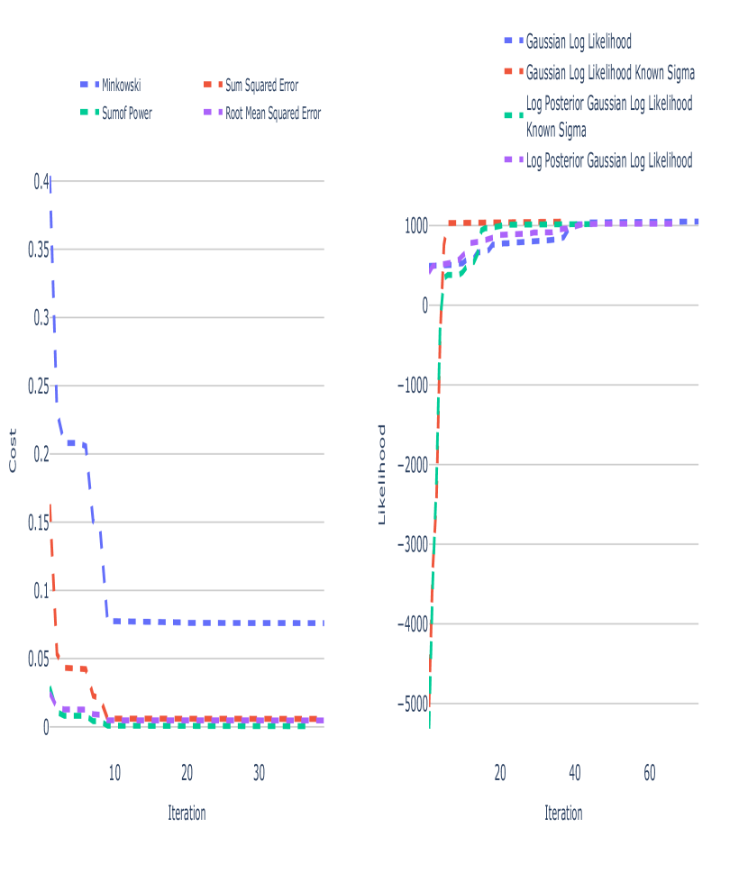
Figure 4: Optimiser convergence using various cost (left) and likelihood (right) functions and the L-BFGS-B algorithm.

Using the same model and parameters, we compare example convergence rates of various algorithms across several categories: gradient-based methods in Figure 5 (left), evolutionary strategies in Figure 5 (middle) and (meta)heuristics in Figure 5 (right) using a mean-squared-error cost function.

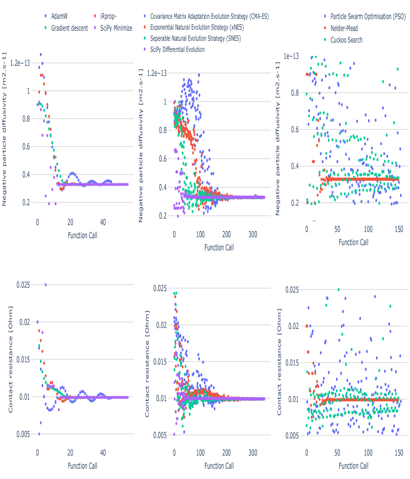
Figure 5: Convergence in parameter values for several optimisation algorithms provided by PyBOP.

We also show the cost function landscapes alongside optimiser iterations in Figure 6, with the three rows showing the gradient-based optimisers (top), evolution strategies (middle), and (meta)heuristics (bottom). Note that the performance of the optimiser depends on the cost landscape, the initial guess or prior, and the hyperparameters for each specific problem.

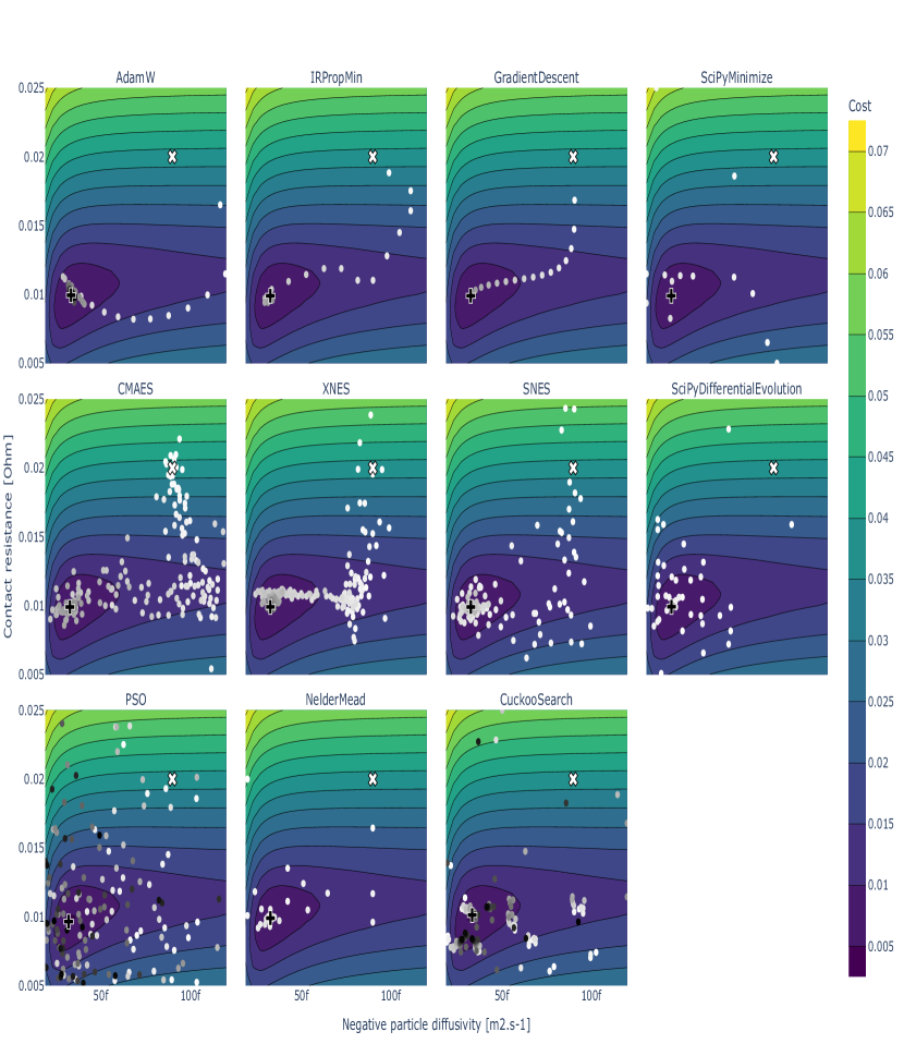
Figure 6: Cost landscape contour plot with corresponding optimisation traces, for several optimisers.

This example parameterisation task can also be approached from a Bayesian perspective, using PyBOP‘s sampler methods. First, we introduce Bayes’ rule,

$$P(\theta|D)=\frac{P(D|\theta)P(\theta)}{P(D)},$$ (6)

where $P(\theta|D)$ is the posterior parameter distribution, $P(D|\theta)$ is the likelihood function, $P(\theta)$ is the prior parameter distribution, and $P(D)$ is the model evidence, or marginal likelihood, which acts as a normalising constant. In the case of maximum likelihood estimation or maximum a posteriori estimation, one wishes to maximise $P(D|\theta)$ or $P(\theta|D)$, respectively, and this may be formulated as an optimisation problem as per Equation 5.

One must use sampling or other inference methods to reconstruct the full posterior parameter distribution, $P(\theta|D)$. The posterior distribution provides information about the uncertainty of the identified parameters, e.g., by calculating the variance or other moments. Monte Carlo methods are used here to sample from the posterior. The selection of Monte Carlo methods available in PyBOP includes gradient-based methods such as no-u-turn (ref-NUTS:2011Hoffman & Gelman, 2011) and Hamiltonian (ref-Hamiltonian:2011Brooks et al., 2011), as well as heuristic methods such as differential evolution (ref-DiffEvolution:2006Braak, 2006), and also conventional methods based on random sampling with rejection criteria (ref-metropolis:1953Metropolis et al., 1953). PyBOP offers a sampler class that provides the interface to samplers, the latter being provided by the probabilistic inference on noisy time-series (PINTS) package. Figure 7 shows the sampled posteriors for the synthetic model described previously, using an adaptive covariance-based sampler called Haario Bardenet (ref-Haario:2001Haario et al., 2001).

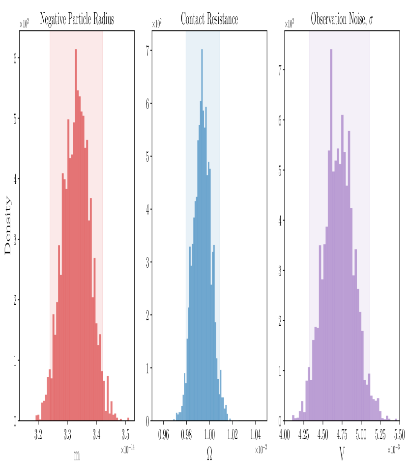
Figure 7: Posterior distributions of model parameters alongside identified noise on the observations. Shaded areas denote the 95th percentile credible interval for each parameter.

Design optimisation

Design optimisation is supported in PyBOP to guide device design development by identifying parameter sensitivities that can unlock improvements in performance. This problem can be viewed in a similar way to the parameterisation workflows described previously, but with the aim of maximising a design-objective cost function rather than minimising a distance-based cost function. PyBOP performs maximisation by minimising the negative of the cost function. In design problems, the cost metric is no longer a distance between two time series, but a metric evaluated on a model prediction. For example, to maximise the gravimetric energy (or power) density, the cost is the integral of the discharge energy (or power) normalised by the cell mass. Such metrics are typically quantified for operating conditions such as a 1C discharge, at a given temperature. In general, design optimisation can be written as a constrained optimisation problem,

$$\min_{\boldsymbol{\theta}\in\Omega}\leavevmode\nobreak\ \mathcal{L}(\boldsymbol{\theta})\leavevmode\nobreak\ \leavevmode\nobreak\ \leavevmode\nobreak\ \textrm{subject to equations (\ref{dynamics}){-}(\ref{initial_conditions}),}$$ (7)

where $\mathcal{L}:\boldsymbol{\theta}\mapsto[0,\infty)$ is a cost function that quantifies the desirability of the design and $\Omega$ is the set of allowable parameter values.

As an example, we consider the challenge of maximising the gravimetric energy density, subject to constraints on two of the geometric electrode parameters (ref-Couto:2023Couto et al., 2023). In this case we use the PyBaMM implementation of the single particle model with electrolyte (SPMe) to investigate the impact of the positive electrode thickness and the active material volume fraction on the energy density. Since the total volume fraction must sum to unity, the positive electrode porosity for each optimisation iteration is defined in relation to the active material volume fraction. It is also possible to update the 1C rate corresponding to the theoretical capacity for each iteration of the design.

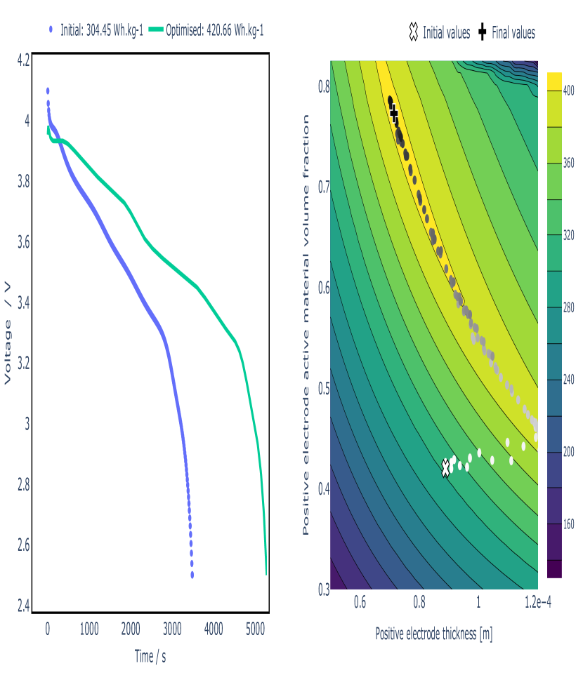
Figure 8: Initial and optimised voltage profiles alongside the gravimetric energy density cost landscape.

Figure 8 (left) shows the predicted improvement in the discharge profile between the initial and optimised parameter values for a fixed-rate 1C discharge selected from the initial design and (right) the Nelder-Mead search over the parameter space.

Conclusion

In this article, the open-source parameter identification and optimisation package, PyBOP has been introduced. This package provides specialised classes and methods to support both physics-based and data-driven parameter identification and optimisation. An example identification workflow has been presented using both point-estimate and distribution-based inference methods for both frequency and time domain forward model predictions. An additional workflow for design optimisation was also presented, showcasing PyBOP as a versatile package capable for researchers and engineers.

References

References

- Aitio, A., Marquis, S. G., Ascencio, P., & Howey, D. (2020). Bayesian parameter estimation applied to the li-ion battery single particle model with electrolyte dynamics IFAC-PapersOnLine, 53(2), 12497–12504. https://doi.org/10.1016/j.ifacol.2020.12.1770
-
Andersson, M., Streb, M., Ko, J. Y., Löfqvist Klass, V., Klett, M.,
Ekström, H., Johansson, M., & Lindbergh, G. (2022). Parametrization of
physics-based battery models from input-output data: A review of
methodology and current research. Journal of Power Sources,
521(November 2021), 230859.
https://doi.org/10.1016/j.jpowsour.2021.230859
-
Braak, C. J. F. T. (2006). A Markov Chain Monte Carlo version of
the genetic algorithm Differential Evolution: Easy Bayesian
computing for real parameter spaces. Statistics and Computing,
16(3), 239–249. https://doi.org/10.1007/s11222-006-8769-1
-
Bradbury, J., Frostig, R., Hawkins, P., Johnson, M. J., Leary, C.,
Maclaurin, D., Necula, G., Paszke, A., VanderPlas, J., Wanderman-Milne,
S., & Zhang, Q. (2018). JAX: Composable transformations of
Python+NumPy programs (Version 0.3.13).
http://github.com/jax-ml/jax
-
Brooks, S., Gelman, A., Jones, G., & Meng, X.-L. (2011). Handbook
of markov chain monte carlo. Chapman; Hall/CRC.
https://doi.org/10.1201/b10905
-
Brosa Planella, F., Ai, W., Boyce, A. M., Ghosh, A., Korotkin, I., Sahu,
S., Sulzer, V., Timms, R., Tranter, T. G., Zyskin, M., Cooper, S. J.,
Edge, J. S., Foster, J. M., Marinescu, M., Wu, B., & Richardson, G.
(2022). A Continuum of Physics-Based Lithium-Ion Battery Models
Reviewed. Progress in Energy, 4(4), 042003.
https://doi.org/10.1088/2516-1083/ac7d31
-
Cabezas, A., Corenflos, A., Lao, J., & Louf, R. (2024). BlackJAX:
Composable Bayesian inference in JAX.
https://arxiv.org/abs/2402.10797
-
Cauchy, A., & others. (1847). Méthode générale pour la
résolution des systemes d’équations simultanées. Comp. Rend.
Sci. Paris, 25(1847), 536–538.
-
Chen, C.-H., Brosa Planella, F., O’Regan, K., Gastol, D., Widanage, W.
D., & Kendrick, E. (2020). Development of experimental techniques for
parameterization of multi-scale lithium-ion battery models.
Journal of The Electrochemical Society, 167(8), 080534.
https://doi.org/10.1149/1945-7111/ab9050
-
Chu, Z., Plett, G. L., Trimboli, M. S., & Ouyang, M. (2019). A
control-oriented electrochemical model for lithium-ion battery, Part
I: Lumped-parameter reduced-order model with constant phase element.
Journal of Energy Storage, 25(August), 100828.
https://doi.org/10.1016/j.est.2019.100828
-
Clerx, M., Robinson, M., Lambert, B., Lei, C. L., Ghosh, S., Mirams, G.
R., & Gavaghan, D. J. (2019). Probabilistic inference on noisy time
series (PINTS). Journal of Open Research Software, 7(1),
23. https://doi.org/10.5334/jors.252
-
Couto, L. D., Charkhgard, M., Karaman, B., Job, N., & Kinnaert, M.
(2023). Lithium-ion battery design optimization based on a dimensionless
reduced-order electrochemical model. Energy, 263(PE),
125966. https://doi.org/10.1016/j.energy.2022.125966
-
DeepMind, Babuschkin, I., Baumli, K., Bell, A., Bhupatiraju, S., Bruce,
J., Buchlovsky, P., Budden, D., Cai, T., Clark, A., Danihelka, I.,
Dedieu, A., Fantacci, C., Godwin, J., Jones, C., Hemsley, R., Hennigan,
T., Hessel, M., Hou, S., … Viola, F. (2020). The
DeepMind JAX Ecosystem. http://github.com/google-deepmind
-
Dhoot, R., Timms, R., & Please, C. (2024). PyBaMM EIS: Efficient
linear algebra methods to determine li-ion battery behaviour (Version
0.1.4). https://www.github.com/pybamm-team/pybamm-eis
-
Doyle, M., Fuller, T. F., & Newman, J. (1993). Modeling of
Galvanostatic Charge and Discharge of the Lithium/Polymer/Insertion
Cell. Journal of The Electrochemical Society, 140(6),
1526–1533. https://doi.org/10.1149/1.2221597
-
Fuller, T. F., Doyle, M., & Newman, J. (1994). Simulation and
optimization of the dual lithium ion insertion cell. Journal of
The Electrochemical Society, 141(1), 1.
https://doi.org/10.1149/1.2054684
-
Haario, H., Saksman, E., & Tamminen, J. (2001). An Adaptive
Metropolis Algorithm. Bernoulli, 7(2), 223.
https://doi.org/10.2307/3318737
-
Hoffman, M. D., & Gelman, A. (2011). The no-u-turn sampler:
Adaptively setting path lengths in hamiltonian monte carlo.
https://arxiv.org/abs/1111.4246
-
Kirk, T. L., Lewis-Douglas, A., Howey, D., Please, C. P., & Jon
Chapman, S. (2023). Nonlinear electrochemical impedance spectroscopy for
lithium-ion battery model parameterization. Journal of The
Electrochemical Society, 170(1), 010514.
https://doi.org/10.1149/1945-7111/acada7
-
Korotkin, I., Timms, R., Foster, J. F., Dickinson, E., & Robinson, M.
(2023). Battery parameter eXchange. In GitHub repository. The
Faraday Institution. https://github.com/FaradayInstitution/BPX
-
Loshchilov, I., & Hutter, F. (2017). Decoupled Weight Decay
Regularization. arXiv.
https://doi.org/10.48550/ARXIV.1711.05101
-
Lu, D., Scott Trimboli, M., Fan, G., Zhang, R., & Plett, G. L. (2021).
Implementation of a physics-based model for half-cell open-circuit
potential and full-cell open-circuit voltage estimates: Part II.
Processing full-cell data. Journal of The Electrochemical
Society, 168(7), 070533.
https://doi.org/10.1149/1945-7111/ac11a5
-
Metropolis, N., Rosenbluth, A. W., Rosenbluth, M. N., Teller, A. H., &
Teller, E. (1953). Equation of State Calculations by Fast
Computing Machines. The Journal of Chemical Physics,
21(6), 1087–1092. https://doi.org/10.1063/1.1699114
-
Miguel, E., Plett, G. L., Trimboli, M. S., Oca, L., Iraola, U., &
Bekaert, E. (2021). Review of computational parameter estimation methods
for electrochemical models. Journal of Energy Storage,
44(PB), 103388. https://doi.org/10.1016/j.est.2021.103388
-
Phan, D., Pradhan, N., & Jankowiak, M. (2019). Composable effects for
flexible and accelerated probabilistic programming in NumPyro.
arXiv Preprint arXiv:1912.11554.
-
Sulzer, V., Marquis, S. G., Timms, R., Robinson, M., & Chapman, S. J.
(2021). Python Battery Mathematical Modelling (PyBaMM). Journal
of Open Research Software, 9(1), 14.
https://doi.org/10.5334/jors.309
-
Tranter, T. G., Timms, R., Sulzer, V., Planella, F. B., Wiggins, G. M.,
Karra, S. V., Agarwal, P., Chopra, S., Allu, S., Shearing, P. R., &
Brett, D. J. l. (2022). Liionpack: A python package for simulating packs
of batteries with PyBaMM. Journal of Open Source Software,
7(70), 4051. https://doi.org/10.21105/joss.04051
-
Verbrugge, M., Baker, D., Koch, B., Xiao, X., & Gu, W. (2017).
Thermodynamic model for substitutional materials: Application to
lithiated graphite, spinel manganese oxide, iron phosphate, and layered
nickel-manganese-cobalt oxide. Journal of The Electrochemical
Society, 164(11), E3243.
https://doi.org/10.1149/2.0341708jes
-
Virtanen, P., Gommers, R., Oliphant, T. E., Haberland, M., Reddy, T.,
Cournapeau, D., Burovski, E., Peterson, P., Weckesser, W., Bright, J.,
van der Walt, S. J., Brett, M., Wilson, J., Millman, K. J., Mayorov, N.,
Nelson, A. R. J., Jones, E., Kern, R., Larson, E., … SciPy 1.0
Contributors. (2020). SciPy 1.0: Fundamental Algorithms for
Scientific Computing in Python. Nature Methods, 17,
261–272. https://doi.org/10.1038/s41592-019-0686-2
-
Wang, A. A., O’Kane, S. E. J., Brosa Planella, F., Houx, J. L., O’Regan,
K., Zyskin, M., Edge, J., Monroe, C. W., Cooper, S. J., Howey, D. A.,
Kendrick, E., & Foster, J. M. (2022). Review of parameterisation and a
novel database (LiionDB) for continuum Li-ion battery models.
Progress in Energy, 4(3), 032004.
https://doi.org/10.1088/2516-1083/ac692c
-
Yang, X.-S., & Suash Deb. (2009). Cuckoo Search via levy flights.
2009 World Congress on Nature & Biologically Inspired
Computing (NaBIC), 210–214.
https://doi.org/10.1109/NABIC.2009.5393690