Bayesian pulsar timing and noise analysis with Vela.jl: an overview

Abstract

We present Vela.jl, an efficient, modular, easy-to-use Bayesian pulsar timing and noise analysis package written in Julia. Vela.jl provides an independent, efficient, and parallelized implementation of the full non-linear pulsar timing and noise model along with a Python binding named pyvela. One-time operations such as data file input, clock corrections, and solar system ephemeris computations are performed by pyvela with the help of the PINT pulsar timing package. Its reliability is ensured via careful design utilizing Julia’s type system, strict version control, and an exhaustive test suite. This paper describes the design and usage of Vela.jl focusing on the narrowband paradigm.

1 Introduction

Pulsars are rotating neutron stars whose electromagnetic radiation is received as periodic pulses. Their high rotational stability makes them excellent celestial clocks, and pulsar timing, the technique of tracking a pulsar’s rotation by measuring the times of arrival (TOAs) of its pulses, is one of the most precise techniques in astronomy (Lorimer & Kramer, 2012). Over the years, pulsar timing has been applied to study a wide array of astrophysical phenomena, such as neutron star equation of state (e.g., Cromartie et al., 2020), tests of theories of gravity (e.g., Voisin et al., 2020), solar wind (e.g., Tiburzi et al., 2021), galactic dynamics (e.g., Perera et al., 2019), etc. Recently, pulsar timing array (PTA: Foster & Backer, 1990) experiments found evidence (e.g., Agazie et al., 2024) for a stochastic gravitational wave background (GWB: Hellings & Downs, 1983) in the nanohertz frequency range with the help of pulsar timing.

In addition to the pulsar rotation, the measured TOAs are also influenced by several deterministic astrophysical processes such as the orbital motion of the Earth, proper motion of the pulsar, solar wind, interstellar dispersion, the orbital motion of the pulsar, etc (Edwards et al., 2006), as well as stochastic processes such as radiometer noise, pulse jitter, rotational irregularities, interstellar medium variability, etc (Agazie et al., 2023a). High-precision pulsar timing requires accurate modeling of all of these effects. A pulsar timing model or pulsar ephemeris provides a mathematical description of the deterministic processes that affect the measured TOAs and is often accompanied by a noise model that describes the stochastic processes therein.

In practice, pulsar timing involves estimating the parameters of a pulsar timing model given a set of TOA measurements, usually in a frequentist setting using a software package such as tempo2 (Hobbs et al., 2006; Edwards et al., 2006) or PINT (Luo et al., 2021; Susobhanan et al., 2024). Noise characterization can be done in a few different ways. In PINT, noise parameters can be estimated together with the timing parameters in a frequentist way (Susobhanan et al., 2024). tempo2 provides plugins like fixData and spectralModel that can estimate some noise parameters by fixing the timing model parameters (Hobbs, 2014). Bayesian noise characterization can be performed using the ENTERPRISE (Johnson et al., 2024) and TEMPONEST (Lentati et al., 2014) packages starting from a post-fit timing model, and is considered standard practice for high-precision timing experiments like PTAs. ENTERPRISE and TEMPONEST differ in how they treat the timing model fit; the former analytically marginalizes a linearized approximation of the timing model (van Haasteren & Levin, 2013), whereas the latter enables inference over the full non-linear timing and noise model. The PINT package also supports Bayesian parameter estimation through pint.fitter.MCMCFitter and pint.bayesian interfaces although their use on large datasets is hampered by slow performance (Luo et al., 2021; Susobhanan et al., 2024). Other packages that have been used for Bayesian pulsar timing and/or noise analysis include libstempo (Vigeland & Vallisneri, 2014), piccard (van Haasteren, 2016), PAL2 (Ellis & van Haasteren, 2017), and FortyTwo (e.g. Chen et al., 2021).

In this paper, we present Vela.jl, a new framework written in Julia (Bezanson et al., 2017) for performing Bayesian inference over the full non-linear timing and noise model. Vela.jl provides an efficient and modular implementation of the pulsar timing and noise model independent of other pulsar timing packages, and supports parallelized evaluation of the pulsar timing likelihood function using multi-threading. We also provide a Python interface named pyvela since Python is more popular among astronomers than Julia. This package is developed with a focus on reliability, performance, and modularity (in that order), employing strict version control (using git) and rigorous testing.

The main objective of Vela.jl is to provide a flexible, robust, modular, well-documented tool for performing Bayesian inference over the full non-linear pulsar timing and noise model. While this functionality is already available in the TEMPONEST package, Vela.jl differs from TEMPONEST in the following ways. (1) TEMPONEST can only be used with the nested sampling packages MULTINEST (Feroz et al., 2009) and PolyChord (Handley et al., 2015), whereas Vela.jl can be used with any Markov Chain Monte Carlo (MCMC: Diaconis, 2009) or nested sampler (Ashton et al., 2022) available in Julia or Python. (2) TEMPONEST uses tempo2 internally to evaluate the timing model, whereas Vela.jl contains an independent implementation of the timing model. (3) TEMPONEST only supports the narrowband timing paradigm, whereas Vela.jl supports both the narrowband and wideband timing paradigms (the application of Vela.jl on wideband data will be discussed in a separate paper). (4) TEMPONEST is a stand-alone application whereas Vela.jl is a library that can be used programmatically alongside various Julia and Python packages.

This paper is arranged as follows. In Section 2, we provide a brief overview of the pulsar timing and noise analysis. In Section 3, we describe the design and implementation of Vela.jl and pyvela. In Section 4, we provide three examples that showcase the functionalities of Vela.jl. Finally, in 5, we summarize our work and discuss the future directions.

2 A brief overview of Bayesian pulsar timing and noise analysis

The fundamental measurable quantity in conventional pulsar timing is the TOA. TOAs are measured by folding the time series pulsar data over a known pulsar period and cross-correlating the resulting integrated pulse profile against a noise-free template (Taylor, 1992), usually after splitting the observation into multiple frequency subbands (this is known as narrowband timing). The more recent wideband timing technique involves measuring a single TOA and a dispersion measure (DM) from an observation by matching the frequency-resolved integrated pulse profile against a two-dimensional template known as a portrait (Pennucci et al., 2014; Pennucci, 2019). Pulsar timing can also be applied directly to integrated pulse profiles (e.g. Lentati et al., 2015), although such techniques are unsuitable for longer pulsar timing campaigns due to intractable data volumes. In the case of high-energy observations, where it is difficult to form integrated pulse profiles or TOAs due to low photon counts, photon arrival times can be used directly for pulsar timing (e.g. Ajello et al., 2022). In this paper, we focus exclusively on the narrowband timing paradigm.

A narrowband TOA $t_{\text{arr}}$ measured at a terrestrial observatory is related to the pulse emission time $t_{\text{em}}$ as

$$t_{\text{arr}}=t_{\text{em}}+\Delta_{\text{B}}+\Delta_{\text{ltt}}+\Delta_{\text{DM}}+\Delta_{\text{scatter}}+\Delta_{\text{GW}}+\Delta_{\odot}+\Delta_{\text{clock}}+\Delta_{\text{jump}}+\mathcal{N}_{\text{R}}+\mathcal{N}_{\text{jitter}}+...\,,$$ (1)

where $\Delta_{\text{B}}$ represents the delays caused by the binary motion of the pulsar including Rømer delay, Shapiro delay, and Einstein delay (Damour & Deruelle, 1986), $\Delta_{\text{ltt}}$ represents a constant light travel time between the pulsar system barycenter and the solar system barycenter at some fiducial epoch, $\Delta_{\text{DM}}$ is the dispersion delay caused by free electrons in the interstellar medium and the solar wind (Backer & Hellings, 1986), $\Delta_{\text{scatter}}$ represents the delay caused by interstellar scattering (Hemberger & Stinebring, 2008), $\Delta_{\text{GW}}$ represents gravitational wave-induced perturbations to the light travel time (Estabrook & Wahlquist, 1975), $\Delta_{\odot}$ represents the delays caused by the motion of the Earth in the solar system including the Rømer delay, Shapiro delay, and Einstein delay (Edwards et al., 2006), $\Delta_{\text{clock}}$ is a series of corrections that converts the TOA measured against an observatory clock to a timescale defined at the solar system barycenter (Hobbs et al., 2006), and $\Delta_{\text{jump}}$ represents instrumental delays. $\mathcal{N}_{\text{R}}$ and $\mathcal{N}_{\text{jitter}}$ are stochastic terms arising from the radiometer noise of the telescope (Lorimer & Kramer, 2012) and random pulse-shape variations (pulse jitter; Parthasarathy et al., 2021), respectively.

Note that each of the delays $\Delta_{X}$ described above can have both deterministic and stochastic components, and such a separation is arbitrary and model-dependent in many cases. The stochastic components corresponding to the delay terms above are orbital variations (due to tidal effects, ablation/accretion from the companion, presence of a third body, etc) (e.g., Arzoumanian et al., 1994), dispersion and scattering variations (due to dynamic and inhomogeneous interstellar medium and variable solar wind) (e.g., Krishnakumar et al., 2015, 2021), the stochastic GW background (e.g., Agazie et al., 2023b), solar system ephemeris errors (e.g., Vallisneri et al., 2020), clock errors (e.g., Tiburzi et al., 2015), etc. Some of these processes, such as stochastic GW background, solar system ephemeris errors, and clock errors, are correlated across multiple pulsars. Such processes usually cannot be distinguished from the rotational irregularities of the pulsar (described below), and are therefore not included in single-pulsar analyses. Additionally, systematic effects such as frequency-dependent profile evolution (Hankins & Rickett, 1986), profile shape change events (e.g. Singha et al., 2021), etc can also influence the measured TOA values if not accurately modeled although they are not true delays.

The emission time $t_{\text{em}}$ estimated using equation (1) can be related to the pulsar rotational phase $\phi$ using the equation (Hobbs et al., 2006)

$$\phi=\phi_{0}+\sum_{n=0}^{n_{F}}\frac{1}{(n+1)!}F_{n}(t_{\text{em}}-t_{0})^{n+1}+\phi_{\text{glitch}}+\phi_{\text{SN}}+...\,$$ (2)

where $\phi_{0}$ represents an arbitrary initial phase, $F_{n}$ represent the pulsar frequency and its derivatives, $n_{F}$ is the number of frequency derivatives, $\phi_{\text{glitch}}$ represents phase corrections due to glitches, and $\phi_{\text{SN}}$ is a stochastic term representing slow stochastic variations in the pulsar rotation known as spin noise. The initial phase $\phi_{0}$ can only be measured modulo an integer number of full rotations, and the constant light travel time $\Delta_{\text{ltt}}$ is fully covariant with $\phi_{0}$ and it is therefore excluded from equation (1) in practice. Further, if a delay term $\Delta_{X}$ is sufficiently small compared to the pulse period $F_{0}^{-1}$, it can be moved into equation (2) as a phase $\Delta_{X}F_{0}$ (e.g., $\Delta_{\text{jump}}$), and if a phase $|\phi_{X}|\ll 1$, it can be moved into equation (1) as a delay $\phi_{X}/F_{0}$ (e.g., $\phi_{\text{SN}}$).

The timing residual $r$ is defined as

$$r=\frac{\phi-\mathcal{N}[\phi]}{F}\,,$$ (3)

where $\mathcal{N}[\phi]$ is the integer closest to $\phi$ and $F={d\phi}/{dt_{\text{arr}}}$ is the topocentric pulse frequency (Hobbs et al., 2006).

The pulsar timing log-likelihood function $\ln L$ can be written as

$$\ln L=-\frac{1}{2}\textbf{r}^{T}\textbf{C}^{-1}\textbf{r}-\frac{1}{2}\ln\det\textbf{C}\,,$$ (4)

where r is an $n_{\text{toa}}$-dimensional column vector containing the timing residuals $r_{i}$ corresponding to the TOAs $t_{i}$, C is the $n_{\text{toa}}\times n_{\text{toa}}$-dimensional TOA covariance matrix, and $n_{\text{toa}}$ is the number of TOAs (Lentati et al., 2014). Pulsar timing in a frequentist setting involves maximizing this likelihood over timing (and possibly noise) parameters (Hobbs et al., 2006; Susobhanan et al., 2024).

The covariance matrix C in general can be a dense symmetric matrix, and it can be computationally expensive to evaluate $\textbf{C}^{-1}$ and $\ln\det\textbf{C}$. To mitigate this computational cost, it is customary to use a reduced-rank approximation of C where

$$\textbf{C}=\textbf{N}+\textbf{U}^{T}\boldsymbol{\Phi}\textbf{U}\,$$ (5)

such that $\textbf{C}^{-1}$ and $\ln\det\textbf{C}$ can be evaluated relatively inexpensively using the Woodbury lemma and the matrix determinant lemma (van Haasteren & Vallisneri, 2014). Here, N is an $n_{\text{toa}}\times n_{\text{toa}}$-dimensional diagonal matrix containing scaled TOA measurement variances $\varsigma_{i}^{2}$ given by

$$\varsigma_{i}^{2}=E_{f}^{2}(\sigma_{i}^{2}+E_{q}^{2})\,,$$ (6)

where $\sigma$ is the measured TOA uncertainty, $E_{f}$ is an EFAC (‘error factor’), and $E_{q}$ is an EQUAD (‘error added in quadrature’) (Lentati et al., 2014). Physically, N represents the fully uncorrelated noise present in the TOAs such as radiometer noise and the uncorrelated part of the pulse jitter noise which depend on the observing system. U is an $n_{\text{toa}}\times p$ dimensional rectangular ‘basis’ matrix and $\boldsymbol{\Phi}$ is a $p\times p$ dimensional diagonal ‘weight’ matrix where $n_{\text{toa}}$ is the number of TOAs and $p$ is the rank of C such that $p\ll n_{\text{toa}}$.

The correlated stochastic processes present in the TOAs are often represented as Gaussian processes which can be written in the form of a delay $\boldsymbol{\Delta}_{X}=\textbf{U}_{X}^{T}\textbf{a}_{X}$, where $\textbf{U}_{X}$ is a ‘basis’ matrix, $\textbf{a}_{X}$ is a vector of amplitudes which are a priori Gaussian-distributed with means $\left\langle\textbf{a}_{X}\right\rangle=0$ and (co)variances $\left\langle\textbf{a}_{X}\textbf{a}_{X}^{T}\right\rangle=\boldsymbol{\Phi}_{X}$, and $\boldsymbol{\Phi}_{X}$ is a diagonal ‘weight’ matrix. Such a process can be included in the timing & noise analysis in two ways. One, they can be included as a delay term in equation (1) along with hyperpriors imposed on the weights $\boldsymbol{\Phi}_{X}$. Alternatively, if the contribution of $\boldsymbol{\Delta}_{X}$ to r is approximated to be linear in $\textbf{a}_{X}$ (which is valid in most cases), the amplitudes $\textbf{a}_{X}$ can be analytically marginalized assuming the above-mentioned Gaussian priors, and this moves the contribution of this process into $\textbf{U}^{T}\boldsymbol{\Phi}\textbf{U}$, leaving only the weights $\boldsymbol{\Phi}_{X}$ as free parameters (Lentati et al., 2014).

For example, the spin noise is usually modeled as a Fourier series such that the elements of $\textbf{U}_{\text{SN}}$ are given by (Lentati et al., 2014)

$$U_{\text{SN};jk}=\begin{cases}\sin\left[\frac{\pi(k+1)(t_{j}-t_{0})}{T_{\text{span}}}\right]&\text{for odd }k\\ \cos\left[\frac{\pi k(t_{j}-t_{0})}{T_{\text{span}}}\right]&\text{for even }k\end{cases}\,,$$ (7)

where $t_{0}$ is some fiducial epoch and $T_{\text{span}}$ is the total span of the TOAs. In this case, the amplitude vector $\textbf{a}_{\text{SN}}$ contains the corresponding Fourier coefficients and the weights contained in $\boldsymbol{\Phi}_{\text{SN}}$ can be interpreted as power spectral densities. See Appendix D for details on how such processes are implemented in Vela.jl. Another example is the ECORR, which represents the component of the pulse jitter noise that is correlated across narrowband TOAs derived from the same observation but uncorrelated otherwise; see Appendix C for further details.

Finally, the log-posterior distribution $\ln P$ of the timing & noise model parameters $\boldsymbol{\alpha}$ given a dataset $\mathfrak{D}$ (containing TOAs, TOA uncertainties, observing frequencies, instrumental configuration information, etc) and a timing & noise model $\mathfrak{M}$ can be written using the Bayes theorem as

$$\ln P[\boldsymbol{\alpha}|\mathfrak{D},\mathfrak{M}]=\ln L[\mathfrak{D}|\boldsymbol{\alpha},\mathfrak{M}]+\ln\Pi[\boldsymbol{\alpha}|\boldsymbol{A},\mathfrak{M}]+\ln\Pi[\boldsymbol{A}|\mathfrak{M}]-\ln Z[\mathfrak{D}|\mathfrak{M}]\,,$$ (8)

where $\Pi$ represents the prior distributions, $\boldsymbol{\alpha}$ represents the free parameters appearing in $\ln L$ (i.e., equations (1–4)), $\boldsymbol{A}$ are the hyperparameters that determine the prior distributions of $\boldsymbol{\alpha}$ (like the weights $\boldsymbol{\Phi}_{X}$), and $Z$ is a normalizing constant known as the Bayesian evidence.

The implementation of the pulsar timing & noise model summarized above (given by equations (1–8)) in Vela.jl is detailed in the next section.

3 The design and implementation of Vela.jl

3.1 Numerical precision

Pulsar timing is one of the few applications where the required numerical precision exceeds the precision provided by the 64-bit floating point type available in most programming languages (e.g., double in C and C++, float in Python, Float64 in Julia). An extended precision floating point type is required to accurately represent the measured TOA values, the pulse phase, and in some cases, the pulsar rotational frequency. Vela.jl uses the Double64 type provided by the DoubleFloats.jl package (Sarnoff et al., 2022), which represents an extended-precision number as a sum of two Float64s (Dekker, 1971), for this purpose. Note that only the TOA values and the rotational phases are represented using Double64, and all other quantities are represented using Float64s because the software-implemented Double64 arithmetic is significantly slower than Float64 arithmetic which is usually hardware-supported.

The rotational Frequency $F_{0}$ is handled manually as a sum of two Float64 numbers as $F_{0}=F_{0}^{\text{big}}+F_{0}^{\text{small}}$, where $F_{0}^{\text{big}}\ll F_{0}^{\text{small}}$ and $F_{0}^{\text{small}}$ is treated as a free parameter where applicable. Handling $F_{0}$ this way significantly simplifies the implementation by allowing all model parameters to have the same underlying floating point type.

The timing residuals computed using Vela.jl agree with those computed using PINT within the $\sim 10$ ns level given identical timing & noise models. An example is shown in Figure 1. This difference is slightly larger than, but of the same order of magnitude as, the difference between PINT and tempo2 residuals shown in Luo et al. (2021). We suspect this difference arises due to the difference in the representation of extended precision numbers.

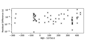
Figure 1: Absolute difference between the timing residuals computed using Vela.jl and PINT for the same timing & noise model given identical model parameters. The two packages agree within $\sim 10$ ns level. The dataset used herein is described in subsection 4.1.

3.2 Quantities

Dimensional analysis is an important tool for ensuring that the mathematical expressions describing the physical processes being studied are correctly translated into code. It turns out that the pulsar timing formula given in equations (1)-(3) can be expressed such that all quantities therein have dimensions of the form $[\textsf{T}^{d}]$ where $d\in\mathbb{Z}$. We give two examples below.

1. The dispersion delay $\Delta_{\text{DM}}=\mathcal{K}\mathcal{D}\nu^{-2}$ where $\mathcal{K}$ is known as the dispersion constant, $\mathcal{D}$ is the dispersion measure (DM; the electron column density along the line of sight), and $\nu$ is the observing frequency in the SSB frame (Lorimer & Kramer, 2012). Although $\mathcal{D}$ has dimensions of $[\textsf{L}^{-2}]$, we can replace this parameter with the dispersion slope $\bar{\mathcal{D}}=\mathcal{K}\mathcal{D}$ which has dimensions of $[\textsf{T}^{-1}]$.

2. The binary Shapiro delay appearing in $\Delta_{\text{B}}$ for an eccentric orbit can be written as (Damour & Deruelle, 1986)

   $$\Delta_{\text{BS}}=\frac{-2GM_{2}}{c^{3}}\log\left[1-e\cos u-\sin\iota([\sin\omega(\cos u-e)+\sqrt{1-e^{2}}\cos\omega\sin u)\right]\,,$$

   where $M_{2}$ is the companion mass, $e$ is the eccentricity, $u$ is the eccentric anomaly, $\iota$ is the orbital inclination, and $\omega$ is the argument of periapsis. Here, the parameter $M_{2}$ has dimensions of $[\textsf{M}]$, but it can be replaced with $\bar{M}_{2}=GM_{2}/c^{3}$ which has dimensions of $[\textsf{T}]$.

The above observation allows us to represent each quantity $q$ appearing in pulsar timing as a combination of a floating point number $x_{q}$ and a compile-time constant integer $d_{q}$, i.e., $q=x_{q}\,\text{s}^{d_{q}}$ where s represents the unit second, and the arithmetic of the $q$ objects follow the usual dimensional analysis rules. Julia’s Just-In-Time compilation allows arithmetic operations using this representation to be executed with almost zero run-time overhead, and this is implemented in the GeometricUnits.jl package as the GQ{d,X<:AbstractFloat} type (‘$<:$’ represents ‘subtype of’). For example, a TOA value has the GQ{1,Double64} type and the observing frequency has the GQ{-1,Float64} type. It also has the benefit of localizing the unit conversion operations to a certain part of the codebase, resulting in easier debugging. It should be noted that time quantities like the TOA values and the various epochs appearing in the timing & noise model are shifted such that the rotational frequency epoch ($t_{0}$ in equation (2)) vanishes.

In comparison, PINT uses the astropy.units module (Robitaille et al., 2013) for this purpose which has a non-negligible computational overhead and tempo2 does not enforce dimensional correctness in this way at all.

3.3 TOAs

A TOA value measured against an observatory clock is usually stored alongside the corresponding measurement uncertainty, observing frequency, a telescope code, and information about the observation setup represented as flags. The various delay and phase corrections as well as the TOA covariance matrix appearing in equations (1)–(4) may depend on any subset of this information.

A TOA is represented in Vela.jl by the TOA type, whose structure is shown in Figure 2. The TOA.value element represents the measured TOA value in the TDB timescale, TOA.error represents the measurement error, TOA.observing_frequency represents the observing frequency in the observatory frame, TOA.pulse_number is the pulse number corresponding to the TOA ($N[\phi]$ in equation (3)), TOA.ephem contains the solar system ephemerides evaluated at the TOA epoch, and TOA.index is an ordinal index. The TOAs are usually stored and distributed as tim files, and Vela.jl uses PINT to read these files to create a collection of TOA objects. The clock corrections needed for converting the TOA value from the observatory timescale to TDB and the solar system ephemerides are precomputed using PINT, which uses astropy (Robitaille et al., 2013) internally; see subsection 3.5. A dataset contains many TOAs, and this is represented as a Vector{TOA} object that stores the TOAs contiguously in memory.

This representation of the TOA is based on the following assumptions: (a) a phase-connected timing solution is available, and (b) the collection of TOAs is immutable. The first assumption allows us to pre-compute TOA.pulse_number. The second assumption allows us to convert the TOA flags, which are string key-value pairs that are expensive to store and manipulate, into inexpensive bit masks specific to the timing model. For example, if the timing model contains $N_{\text{jump}}$ observing system-dependent jumps ($\Delta_{\text{jump}}$) which depend on some TOA flags, the same information can be represented as an $N_{\text{toa}}\times N_{\text{jump}}$-dimensional bit mask (this is stored within the timing model instead of the TOAs).

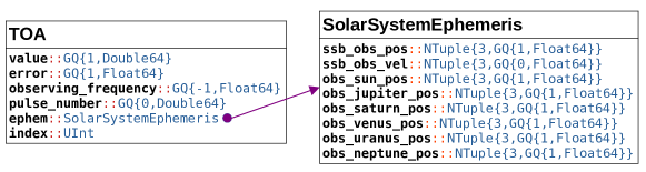
Figure 2: The structure of the TOA type. TOA.value is in the TDB timescale. The SolarSystemEphemeris type contains 3-tuples representing the position and velocity of the observatory with respect to the SSB (SolarSystemEphemeris.ssb_obs_pos and SolarSystemEphemeris.ssb_obs_vel), and the positions of various solar system objects with respect to the observatory. The clock corrections required for computing TOA.value and the solar system ephemerides are evaluated with the help of PINT. UInt is an unsigned integer.

3.4 The timing & noise model

We begin this section by writing down a version of equation (1) that is closer to how it is implemented in practice. Some of the delays are omitted for simplicity.

$$t_{\text{em}}+\mathcal{N}={t}_{\text{tdb}}-\Delta_{\odot}(\bar{t}_{\text{tdb}})-\Delta_{\text{DM}}(\bar{t}_{\text{ssb}})-\Delta_{\text{B}}(\bar{t}_{\text{dd}})-...\,,$$ (9)

where $\bar{t}_{X}$ represents a TOA ($t_{X}$) along with its uncertainty ($\sigma_{X}$), observing frequency ($\nu_{X}$), etc after a correction step $X$, $\mathcal{N}$ represents the uncorrelated noise present in the data, $t_{\text{tdb}}=t_{\text{arr}}-\Delta_{\text{clock}}(\bar{t}_{\text{arr}})$ is the TOA in the TDB timescale, $t_{\text{ssb}}=t_{\text{tdb}}-\Delta_{\odot}(\bar{t}_{\text{tdb}})$ is the barycentered TOA, $\nu_{\text{ssb}}=\nu_{\text{tdb}}(1-\delta_{\odot}(\bar{t}_{\text{tdb}}))$ is the barycentered observing frequency, $\delta_{\odot}$ is a Doppler factor due to solar system motion, and $t_{\text{dd}}=t_{\text{ssb}}-\Delta_{\text{DM}}(\bar{t}_{\text{ssb}})$ is the dedispersed TOA. The above expression makes it clear that the delay corrections must be applied in a specific order: solar system delays, interstellar dispersion delays, pulsar binary delays, etc. Then, the different phase terms in equation (2) are computed.

In Vela.jl, the different delay and phase terms in equations (1) and (2) and the TOA uncertainty corrections in equation (6) that are uncorrelated across TOAs are implemented as subtypes of the Component type. The hierarchy and descriptions of various Component types available in Vela.jl are given in Appendix A. Each Component type has an associated correct_toa() method which computes the corresponding delay, phase, Doppler factor, uncertainty correction, etc. The corrected TOA $t_{\text{em}}$, the phase $\phi(t_{\text{em}})$, and the scaled TOA uncertainty $\varsigma$, and the topocentric frequency $F$ are computed by successively applying these methods in the correct order. Finally, the timing residuals are computed using equation (3).

The likelihood function is computed from the timing residuals with the help of a Kernel object which represents the matrix operations present in equation 4. Two Kernel types are available currently. WhiteNoiseKernel represents the case when only uncorrelated (white) noise is present in the TOAs, i.e., the covariance matrix $\textbf{C}=\textbf{N}$ is diagonal. In this case, $\ln L$ can be evaluated with $\mathcal{O}(N_{\text{toa}})$ time complexity. EcorrKernel represents the case when only time-uncorrelated noise (i.e., white noise and ECORR) is present. It turns out that $\ln L$ can be evaluated with $\mathcal{O}(N_{\text{toa}})$ time complexity in the latter case also, see Appendix C for details.

The timing & noise model is represented in Vela.jl as the TimingModel type, shown in Figure 3. In addition to the Components and the Kernel described above, a TimingModel object also contains a ParamHandler object that contains information about the model parameters and an ordered collection of Prior objects which implement the prior distributions appearing in equation 8; see Appendix B for more details.

Vela.jl provides functions that return callable objects which compute the log-likelihood (get_lnlike_func()), the log-prior (get_lnprior_func()), the prior transform (get_prior_transform_func()), and the log-posterior (get_lnpost_func()). The outputs of these functions can be passed on to any MCMC or nested sampler.

Three parallelization paradigms are provided for the log-likelihood and log-posterior computation. By default, the computation is parallelized across TOAs using multi-threading (equations (4) and (C5) are trivially parallelizable this way). Some ensemble samplers like emcee support vectorized execution of the posterior distribution across multiple points in the parameter space, and Vela.jl provides the option to do this parallelly using multiple threads. Alternatively, Vela.jl also provides serial versions of the same functions for cases where the sampler itself implements parallelization, e.g., using Message Passing Interface (MPI: Gropp et al., 1996).

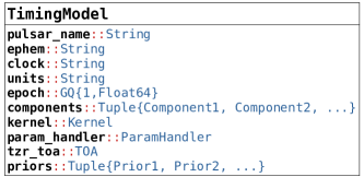
Figure 3: The structure of the TimingModel type. pulsar_name stores the name of the pulsar. ephem is the name of the solar system ephemeris model. clock is the name of the realization of the TT timescale used in clock corrections (e.g., TT(BIPM2021)); see Hobbs et al. (2006). units is the timescale of TOA.value (only TDB is supported). epoch is the rotational frequency epoch. The components tuple contains Component objects representing different terms in the timing & noise model that are uncorrelated across TOAs. Kernel is an object representing the computation in equation (4) including the various contributions to the TOA covariance matrix C. param_handler contains information about the different parameters appearing in the timing & noise model. tzr_toa is a fiducial TOA with respect to which the rotational phase is measured (‘tzr’ stands for ‘t-zero’). priors is a tuple that contains the prior distributions for the free model parameters.

3.5 The pyvela Interface

We provide a Python interface for Vela.jl called pyvela for easy usage developed using JuliaCall/PythonCall (Rowley, 2022). This is useful because Pulsar Astronomers tend to be more familiar with Python than Julia, and because Python offers a wider choice of sampling packages than Julia.

The SPNTA class (SPNTA stands for single-pulsar noise & timing analysis) in pyvela reads a pair of par and tim files, performs the clock corrections and solar system ephemeris computations with the help of PINT, constructs the prior distributions (see Appendix B), and creates a pair of TimingModel and Vector{TOA} objects described above. It also provides a convenient interface for evaluating the log-likelihood, log-prior, prior transform, and log-posterior functions. An example code snippet using pyvela with the MCMC sampler emcee (Foreman-Mackey et al., 2013) is shown in Figure 4, and an example using pyvela with the nested sampler nestle (Barbary, 2021) is shown in Figure 5.

⬇

1from pyvela import SPNTA

2import emcee

3import numpy as np

4

5spnta = SPNTA(

6 parfile="NGC6440E.par",

7 timfile="NGC6440E.tim",

8 custom_priors="NGC6440E_priors.json",

9)

10

11nwalkers = spnta.ndim * 5

12p0 = np.array([

13 spnta.prior_transform(cube)

14 for cube in np.random.rand(nwalkers, spnta.ndim)

15])

16

17sampler = emcee.EnsembleSampler(

18 nwalkers,

19 spnta.ndim,

20 spnta.lnpost,

21)

22

23sampler.run_mcmc(p0, 6000, progress=True)

24samples_raw = sampler.get_chain(flat=True, discard=1000, thin=50)

25

26samples = spnta.rescale_samples(samples_raw)

Figure 4: An example code snippet demonstrating the pyvela interface with the MCMC sampler emcee. User-defined priors are read from a JSON file (see Appendix B). The emcee.EnsembleSampler object is initialized with samples drawn from the prior distribution with the help of SPNTA.prior_transform(). The samples are originally in Vela.jl’s internal units. They are converted into their commonly used units using SPNTA.rescale_samples().

⬇

1from pyvela import SPNTA

2import nestle

3import numpy as np

4

5spnta = SPNTA(

6 parfile="NGC6440E.par",

7 timfile="NGC6440E.tim",

8 custom_priors="NGC6440E_priors.json",

9)

10

11results = nestle.sample(

12 spnta.lnlike,

13 spnta.prior_transform,

14 spnta.ndim,

15 method="multi",

16 npoints=500,

17 dlogz=0.001,

18 callback=nestle.print_progress,

19)

20

21samples_raw = nestle.resample_equal(results.samples, results.weights)

22samples = spnta.rescale_samples(samples_raw)

23

24log_evidence = results.logz

Figure 5: An example code snippet demonstrating the pyvela interface with the nested sampler nestle. method="multi" invokes the MultiNest algorithm (Feroz et al., 2009).

A schematic diagram that summarizes how Vela.jl works is shown in Figure 6.

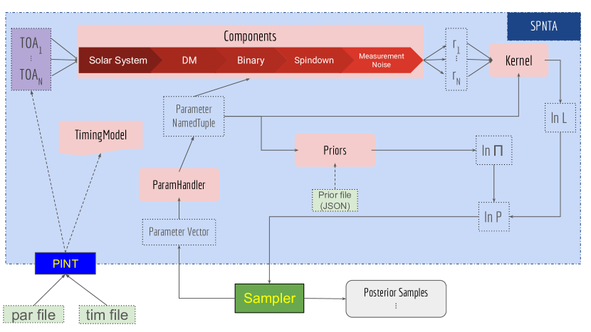
Figure 6: A schematic diagram summarizing Vela.jl’s architecture. Components, Kernel, Priors, and ParamHandler are parts of the TimingModel.

4 Application to simulated datasets

In this section, we demonstrate the application of Vela.jl on two simulated datasets. These are generated using the pint.simulation module (Susobhanan et al., 2024) based on certain real datasets.

4.1 PSR J1748-2021E (NGC 6440E)

PSR J1748-2021E is an isolated pulsar located in the globular cluster NGC 6440. The simulated dataset is generated based on a real dataset presented in Freire et al. (2008) and contains 61 TOAs taken using the Green Bank Telescope from 2005 to 2006 with observing frequencies in the range 1550-1212 MHz.

We convert the TOAs from the observatory timescale to TDB with the help of the BIPM2021 realization of the TT timescale and the DE421 solar system ephemeris. The timing & noise model includes solar system delays, interstellar dispersion, spindown, and a global EFAC that scales the measured TOA uncertainties. This model has 7 free parameters.

We run the Bayesian analysis using Vela.jl with emcee, which implements the affine-invariant ensemble sampler algorithm (Foreman-Mackey et al., 2013) (see Figure 4 for the Python script). The prior distribution of the global EFAC is LogNormal[0,0.25] and that of the overall phase offset is Uniform[-0.5,0.5]. ‘Cheat’ prior distributions, i.e., uniform distributions centered at the maximum likelihood values obtained using PINT whose widths are 10 times the frequentist uncertainties, are used for all other parameters (see Appendix B). We have checked that increasing the width of the ‘cheat’ priors does not appreciably alter the posterior distribution.

We repeat this analysis using the pint.bayesian module (Susobhanan et al., 2024) with emcee for comparison. This is computationally feasible due to the small size of the dataset. The posterior distributions and post-fit residuals obtained from this exercise are shown in Figure 7, and show good agreement between the posterior distributions and post-fit residuals obtained using Vela.jl and pint.bayesian. Further, the estimated parameters agree with the injected parameters within 2$\sigma$ uncertainties.

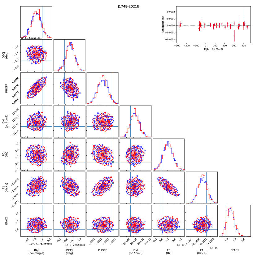
Figure 7: Bayesian timing & noise analysis results for a simulated dataset of PSR J1748$-$2021E. The plotted parameters are source coordinates (RAJ, DECJ), overall phase offset (PHOFF), dispersion measure (DM), rotational phase and its derivative (F0, F1), and a global EFAC (EFAC1). The results obtained using Vela.jl are plotted in red, and those obtained using PINT are plotted in blue. The inset shows the timing residuals computed using the median values of the posterior samples. A value of 61.4854765543713046 Hz has been subtracted from the rotational frequency F0.

4.2 PSR J1909$-$3744

PSR J1909$-$3744 is a millisecond binary pulsar observed as part of multiple PTA campaigns. The simulated dataset used in this section is generated based on a subset of the narrowband data of J1909$-$3744 published as part of the Indian Pulsar Timing Array data release 1 (InPTA DR1: Tarafdar et al., 2022). It contains 361 TOAs measured using the Giant Metrewave Radio Telescope (GMRT) during 2020-2021 in two frequency bands (300-500 MHz and 1260-1460 MHz). Notably, we have injected the dispersion measure variations based on the epoch-wise DM measurements given in the InPTA DR1.

We convert the TOAs from the observatory timescale to TDB with the help of the BIPM2019 realization of the TT timescale and the DE440 solar system ephemeris. The timing & noise model used to fit the simulated data includes solar system delays (including parallax and proper motion), dispersion measure variations modeled as a combination of a Taylor series (up to the second DM derivative) and a Fourier series Gaussian process with 40 harmonics (see Appendix D), the ELL1 model for a nearly circular binary, pulsar spindown, and EFACs and EQUADs applied to the two observing frequency bands. This model has 104 free parameters in total.

The prior distributions of some of the parameters are given in Table 1. The priors for the scaled Fourier amplitudes of the DM noise are unit normal distributions as discussed in Appendix D. ‘Cheat’ priors are used for the other parameters with width 40 times their frequentist uncertainty. We have checked that increasing the width of the ‘cheat’ priors does not appreciably alter the posterior distribution.

Parameter	Description	Prior
M2	Companion mass ($M_{\odot}$)	Uniform distribution around the IPTA DR2 measurement
		with width 40 times the corresponding uncertainty
SINI	Orbital inclination	$\Pi(\sin\iota)=\frac{\sin\iota}{\sqrt{1-\sin^{2}\iota}}$ (see Appendix B)
TNDMAMP	Spectral log-amplitude of DM noise	LogUniform[$10^{-18}$, $10^{-12}$]
TNDMGAM	Spectral index of DM noise	Uniform[0.5, 7]
PHOFF	Overall phase offset	Uniform[-0.5, 0.5]
EFAC	Scale factor for TOA uncertainties	LogNormal[0, 0.25]
EQUAD	TOA uncertainty correction	LogUniform[$10^{-3}$, $10$]
	added in quadrature ($\mu$s)

Table 1: The prior distributions used for analyzing the simulated dataset of PSR J1909$-$3744. ‘Cheat’ priors are used for timing parameters not mentioned here. IPTA DR2 is the International Pulsar Timing Array Data Release 2 (Perera et al., 2019).

The posterior samples were obtained using emcee, and the results of this analysis are plotted in Figure 8. We see that some of the estimated parameters do not agree well with their injected values. This may be because the DM model is not adequately modeling some of the short-timescale DM variations (see inset of Figure 8).

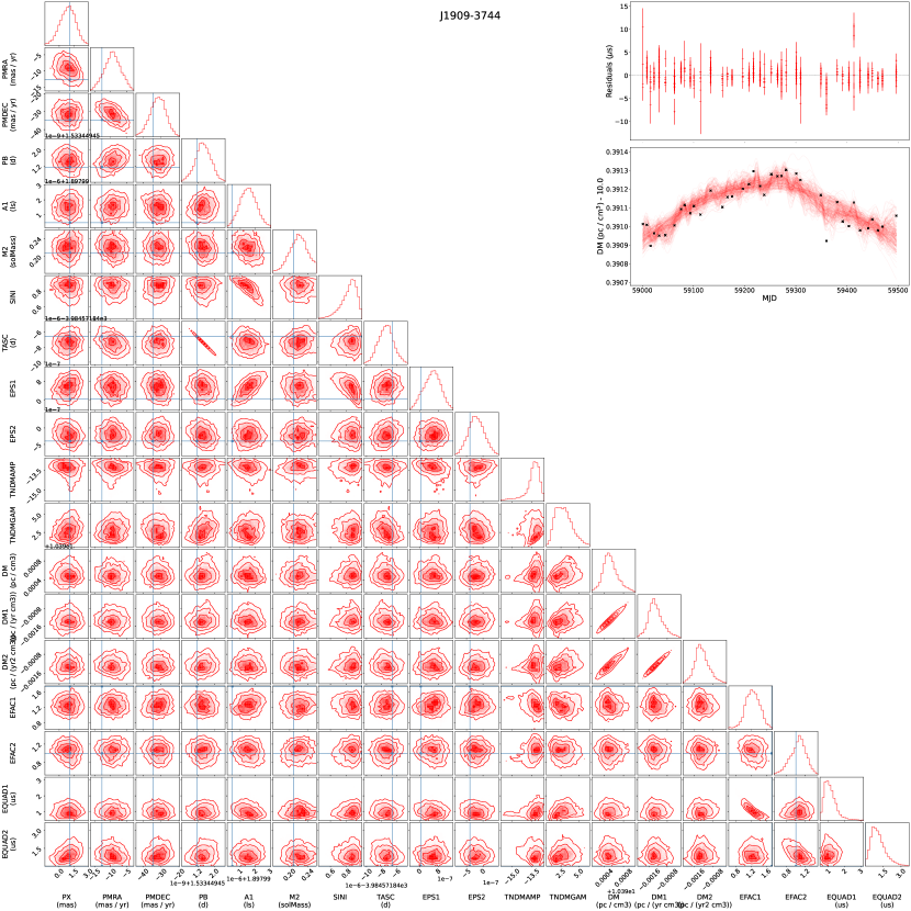
Figure 8: Bayesian timing & noise analysis results for a simulated dataset of PSR J1909-3744. The plotted parameters are parallax (PX), proper motion (PMRA, PMDEC), orbital period (PB), projected semi-major axis (A1), companion mass (M2), sine-inclination (SINI), epoch of ascending node (TASC), Laplace-Lagrange parameters (EPS1, EPS2), dispersion measure and its derivatives (DM, DM1, DM2), power law spectral parameters of the DM noise (TNDMAMP, TNDMGAM), EFACs, and EQUADs. The two EFACs and EQUADs correspond to the 300-500 MHz band and the 1260-1460 MHz band in that order. The source coordinates (RAJ, DECJ), the rotational frequency and its derivative (F0, F1), the overall phase offset (PHOFF), and the Fourier amplitudes of the DM noise are not plotted. The vertical and horizontal lines represent the injected values. The estimated parameters of astrometric and binary parameters are consistent with the injected values within $3\sigma$ uncertainties. Note that a Fourier series Gaussian process model was used for the analysis whereas the injected DM values were taken from real epoch-wise measurements. The inset shows post-fit residuals in the top panel. The bottom panel of the inset shows the injected DM time series (black points) and 200 random realizations of the DM time series drawn from the posterior distribution.

5 Summary & Future directions

We have developed a new package for performing Bayesian single-pulsar timing & noise analysis named Vela.jl. This package is written in Julia and provides an efficient and parallelized implementation of the non-linear timing & noise model along with a Python interface named pyvela. It uses PINT to read par & tim files, apply clock corrections to the TOAs, and compute solar system ephemerides but provides an independent implementation of the timing & noise model. Given a set of TOAs and a timing & noise model, Vela.jl provides an intuitive interface for computing the log-likelihood, log-prior, prior transform, and log-posterior functions that are compatible with various MCMC and nested samplers available in Julia and Python. The architecture of Vela.jl is summarized below.

1. Dimensionful quantities are converted to a form that has dimensions $[\textsf{T}^{d}]$ and represented using GQ{d,X<:AbstractFloat} types. Values that require extended precision are stored using the Double64 type.

2. Clock-corrected TOAs and their metadata along with the pre-computed solar system ephemerides are stored using the TOA type.

3. The timing & noise model is represented using the TimingModel type. It contains:

   1. Components which represent various physical and instrumental effects that are uncorrelated across TOAs.

   2. A Kernel which represents the log-likelihood computation and correlated noise if any.

   3. Priors which represent the prior distributions of free model parameters.

   4. A ParamHandler which converts the parameter values provided by the sampler into a representation that can be accessed efficiently.

4. The pyvela interface provides a Python binding to Vela.jl. It contains the SPNTA class which

   1. Reads the par and tim files, computes clock corrections and solar system ephemerides, and constructs the TimingModel and TOA objects.

   2. Provides methods that compute the log-likelihood, log-prior, prior transform, and log-posterior that can be passed into samplers.

We demonstrated the usage of Vela.jl using two example datasets. In the case of the smaller dataset, we showed that the parameter estimation results are consistent with those estimated using PINT.

Vela.jl was developed to be a more user-friendly and flexible alternative to TEMPONEST, and it should complement the capabilities of ENTERPRISE which does not allow the exploration of the full non-linear timing model. Vela.jl will be a useful tool for analyzing the various pulsar timing datasets, especially those of high-precision experiments such as PTAs that are rapidly growing in volume and sensitivity.

The planned future development wishlist for Vela.jl is as follows.

1. Develop a vibrant community of users and developers.

2. Implement wideband timing (Alam et al., 2021) (under development).

3. Implement photon domain timing for high-energy pulsar timing (Pletsch & Clark, 2015) and enable simultaneous analysis of radio TOA data and high-energy photon data.

4. Implement a sampler that is tuned to the pulsar timing & noise analysis. Possible avenues to explore are Gibbs sampling (e.g. Laal et al., 2023) and Hamiltonian Monte Carlo (e.g. Freedman et al., 2023).

5. Implement automatic differentiation using a tool like Zygote.jl (Innes, 2018). This is crucial for implementing Hamiltonian Monte Carlo.

6. Implement a fitter for PINT using Vela.jl as a backend. This should be useful in cases where PINT is too slow, especially for noise estimation (Susobhanan et al., 2024).

7. Implement timing model components that are currently unavailable in Vela.jl, such as the DDGR and ELL1k binary models (Damour & Deruelle, 1986; Susobhanan et al., 2018), advanced solar wind models (Hazboun et al., 2022; Susarla et al., 2024), etc.

Data Availability

The simulated datasets used in this work and the Jupyter notebooks used to analyze them are available at … The dataset of PSR J1748$-$2021E used to generate the simulated dataset is distributed with PINT as an example dataset at https://github.com/nanograv/PINT/. The dataset of PSR J1909$-$3744 used to generate the simulated dataset is available as part of the InPTA DR1 at https://github.com/inpta/InPTA.DR1/.

Appendix A Component types available in Vela.jl

Figure 9 shows the hierarchy of the various abstract subtypes of Component. Concrete Component types are listed in Table 2.

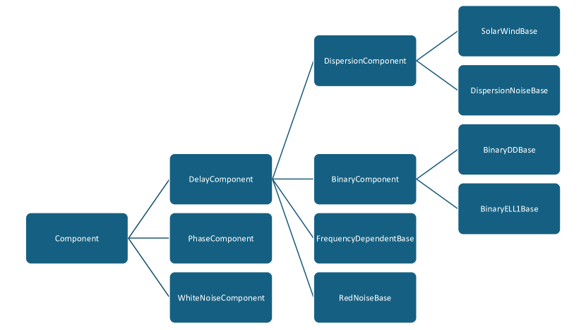
Figure 9: The hierarchy of Component base types. See Table 2 for their implemented concrete subtypes.

Component & Base Type PINT Equivalent(s) Description & Reference SolarSystem AstrometryEquatorial Solar system delays (Rømer, parallax, and Shapiro) and Doppler <: DelayComponent AstrometryEcliptic correction (Edwards et al., 2006) SolarSystemShapiro SolarWindDispersion SolarWindDispersion Solar wind dispersion assuming spherical symmetry <: SolarWindBase (Edwards et al., 2006) DispersionTaylor DispersionDM Taylor series representation of interstellar dispersion <: DispersionComponent (Backer & Hellings, 1986) DMWaveX DMWaveX Unconstrained Fourier series representation of interstellar dispersion <: DispersionComponent variations (Susobhanan et al., 2024) PowerlawDispersionNoiseGP PLDMNoise Fourier series Gaussian process representation of interstellar dispersion <: DispersionNoiseBase variations with a power law spectrum (Lentati et al., 2014) DispersionOffset FDJumpDM System-dependent dispersion measure offset <: DispersionComponent ChromaticTaylor ChromaticCM Taylor series representation of a chromatic delay <: ChromaticComponent (Hemberger & Stinebring, 2008) CMWaveX CMWaveX Unconstrained Fourier series representation of variable chromatic delay <: ChromaticNoiseBase PowerlawChromaticNoiseGP PLChromNoise Fourier series Gaussian process representation of variable chromatic <: ChromaticNoiseBase delay with a power law spectrum (Lentati et al., 2014) BinaryDD BinaryDD Parameterized model for eccentric binaries with relativistic effects <: BinaryDDBase BinaryBT (Damour & Deruelle, 1986) BinaryDDH BinaryDDH Similar to BinaryDD, but with an orthometric representation of Shapiro <: BinaryDDBase delay suitable for low-inclination systems (Weisberg & Huang, 2016) BinaryDDK BinaryDDK Similar to BinaryDD, but with Kopeikin corrections due to parallax <: BinaryDDBase and proper motion (Kopeikin, 1995, 1996) BinaryDDS BinaryDDS Similar to BinaryDD, but with an alternative parameterization of <: BinaryDDBase Shapiro delay suitable for almost edge-on systems (Rafikov & Lai, 2006) BinaryELL1 BinaryELL1 Parameterized model for almost circular binaries with relativistic <: BinaryELL1Base effects (Lange et al., 2001) BinaryELL1H BinaryELL1H Similar to BinaryELL1, but with an orthometric representation of <: BinaryELL1Base Shapiro delay (Freire & Wex, 2010) FrequencyDependent FD Phenomenological model for apparent delays caused by un-modeled <: FrequencyDependentBase profile evolution (Arzoumanian et al., 2015) FrequencyDependentJump FDJump Similar to FrequencyDependent, but accounts for experiment-dependent <: FrequencyDependentBase differences in modeling profile evolution (Susobhanan et al., 2024) WaveX WaveX Apparent delay due to rotational irregularities of the pulsar <: RedNoiseBase represented as an unconstrained Fourier series (Susobhanan et al., 2024) PowerlawRedNoiseGP PLRedNoise Rotational irregularities of the pulsar represented as a Fourier <: RedNoiseBase series Gaussian process with power law spectrum (Lentati et al., 2014) Spindown Spindown Taylor series representation of the pulsar spin-down (Hobbs et al., 2006) <: PhaseComponent Glitch Glitch Pulsar glitches (Hobbs et al., 2006) <: PhaseComponent PhaseOffset PhaseOffset Overall initial phase (Susobhanan et al., 2024) <: PhaseComponent PhaseJump PhaseJump System-dependent phase offsets (Hobbs et al., 2006) <: PhaseComponent MeasurementNoise ScaleToaErrors Corrections to the measured TOA uncertainties (Lentati et al., 2014) <: WhiteNoiseComponent

Table 2: Timing & noise model components available in Vela.jl. See Section 2 for an overview of the timing & noise model and Section 3.4 for its implementation in Vela.jl. See Figure 9 for the hierarchy of base types. The ‘<:’ symbol represents ‘subtype of’.

Appendix B Prior distributions

In principle, the prior for each parameter should be set strictly based on our prior knowledge. Indeed, we may have prior information on some of the parameters from previous timing experiments, VLBI campaigns (e.g. Deller et al., 2016), detection of counterparts in other parts of the electromagnetic spectrum (e.g. Kaplan et al., 2018), etc. Or priors may be estimated from population statistics using a catalog like psrcat (Manchester et al., 2005).

However, for many parameters, pulsar timing provides so much signal-to-noise ratio (S/N) that the effect of the prior on the posterior distribution is entirely negligible provided the prior is sufficiently broad. This is the case for parameters like $F_{0}$, $F_{1}$, source coordinates, etc even for small timing datasets. In the context of analytic marginalization of linearized timing model parameters, it is customary to assume uninformative infinitely broad Gaussian priors (van Haasteren & Levin, 2013). On the other hand, given the insensitivity of the posterior distribution on the priors on some of the timing model parameters, ‘cheat’ priors, namely uniform distributions centered around the frequentist estimate whose width is several times (e.g., 10x) the frequentist uncertainty, have also been used (e.g. Lentati et al., 2014). In cases like the amplitudes of a Fourier series Gaussian process (e.g., PowerlawRedNoiseGP), the priors are defined by the model itself.

Care must be taken to ensure that the data provides enough S/N for the parameter for the ‘cheat’ prior distribution to be valid, lest we effectively do circular analysis (Kriegeskorte et al., 2009). A ‘cheat’ prior can also become invalid if the parameter has a physical range, e.g., the sin-inclination of the binary orbit $\sin\iota\in[0,1]$, and the frequentist measurement is close to the physical upper/lower bound. (See Table 3 for physically motivated priors on different parameterizations of the inclination $\iota$.)

In cases where a physically motivated prior can be analytically derived, Vela.jl uses those priors. For other parameters, ‘cheat’ priors with a user-defined width are used by default. Crucially, the user may override any of these defaults with the help of univariate distributions defined in Distributions.jl. The pyvela interface accepts such user-defined univariate prior distributions in the form of a JSON file (see Figure 10 for an example). Finally, if the prior distributions described above are inadequate, the user also has the flexibility of defining their own prior distributions outside the Vela.jl framework since Vela.jl is not closely coupled to any sampler.

Parameter	Binary	Definition	Prior distribution
name	Models		Support	PDF	CDF	Quantile
KIN	BinaryDDK	Orbital inclination ($\iota$)	$[0,\pi/2]$	$\sin\iota$	$1-\cos\iota$	$\arccos\left(1-q\right)$
SINI	BinaryDD	$s=\sin\iota$	$[0,1]$	$\frac{s}{\sqrt{1-s^{2}}}$	$1-\sqrt{1-s^{2}}$	$\sqrt{\left(2-q\right)q}$
	BinaryELL1
STIGMA	BinaryDDH	$\varsigma=\frac{\sin\iota}{1+\cos\iota}$	$[0,1]$	$\frac{4\varsigma}{\left(1+\varsigma^{2}\right)^{2}}$	$\frac{2\varsigma^{2}}{1+\varsigma^{2}}$	$\sqrt{\frac{q}{2-q}}$
	BinaryELL1H
SHAPMAX	BinaryDDS	$S=-\ln(1-\sin\iota)$	$[0,\infty)$	$\frac{1-e^{-S}}{\sqrt{2e^{S}-1}}$	$1-e^{-S}\sqrt{2e^{S}-1}$	$\ln\left[\frac{\sqrt{2q-q^{2}}+1}{(q-1)^{2}}\right]$

Table 3: Physically motivated prior distributions for different parameterizations of the orbital inclination $\iota$ assuming that $\cos\iota$ is uniformly distributed in $[0,1]$. The support, probability density function (PDF), cumulative distribution function (CDF), and quantile function (relevant for computing the prior transform) are listed. See Table 2 for the definitions of different binary models.

⬇

1{

2 "EFAC": {

3 "distribution": "LogNormal",

4 "args": [0.0, 0.5]

5 },

6 "EQUAD": {

7 "distribution": "LogUniform",

8 "args": [0.01, 2.0]

9 }

10 "M2": {

11 "distribution": "Normal",

12 "args": [1.0, 0.02],

13 "lower": 0.0

14 }

15}

Figure 10: An example of the user-defined prior distributions represented in the JSON format. ‘distribution’ should be a distribution available in the Distributions.jl package (Besançon et al., 2021). ‘args’ contains the arguments to construct a distribution object. The ‘upper’ and ‘lower’ options allow the distribution to be truncated. Only univariate distributions with constant hyperparameters are supported. The arguments and the upper and lower bounds have the same units used in the par files where applicable. For example, the prior distribution for M2 above corresponds to a normal distribution with mean 1 $M_{\odot}$ and standard deviation 0.02 $M_{\odot}$ truncated such that M2 $>$ 0.

Appendix C Representation of ECORR

In this section we describe the representation of the ECORR noise used in Vela.jl following Johnson et al. (2024) and Susobhanan et al. (2024). When ECORR is the only correlated contribution to C (i.e., the time-correlated noise components, if any, are included as a delay or phase correction rather than in C), assuming that there are no overlapping ECORR groups, C can be written as

$$\textbf{C}=\textbf{N}+\sum_{ab}c_{a}\textbf{v}_{ab}\textbf{v}_{ab}^{T}\,,$$ (C1)

where $c_{a}^{2}$ is the ECORR weight, the index $a$ represents the different systems for which the ECORRs are assigned, $b$ represents different observing epochs, and N is a diagonal matrix. The $\textbf{v}_{ab}$ are vectors that have $1$s for TOAs belonging to the system $a$ and epoch $b$, and $0$s otherwise. It is clear that C is block-diagonal in this case, and each block $\textbf{C}_{ab}$ can be written as

$$\textbf{C}_{ab}=\textbf{N}_{ab}+c_{a}\textbf{v}_{ab}\textbf{v}_{ab}^{T}\,,$$ (C2)

where $\textbf{N}_{ab}$ is the portion of N corresponding to the system $a$ and epoch $b$. The inverse and determinant of $\textbf{C}_{ab}$ can be written as

$$\textbf{C}_{ab}^{-1} =\textbf{N}_{ab}^{-1}-\frac{c_{a}^{2}\textbf{N}_{ab}^{-1}\textbf{v}_{ab}\textbf{v}_{ab}^{T}\textbf{N}_{ab}^{-1}}{1+c_{a}^{2}\textbf{v}_{ab}^{T}\textbf{N}_{ab}^{-1}\textbf{v}_{ab}}\,,$$ (C3)

$$\det\textbf{C}_{ab} =\det\textbf{N}_{ab}\times\left(1+c_{a}^{2}\textbf{v}_{ab}^{T}\textbf{N}_{ab}^{-1}\textbf{v}_{ab}\right)\,.$$ (C4)

Defining an inner product $\left(\textbf{x}_{ab}|\textbf{y}_{ab}\right)=\textbf{x}_{ab}^{T}\textbf{N}_{ab}^{-1}\textbf{y}_{ab}$ and writing the log-likelihood function as a sum $\ln L=\sum_{ab}\ln L_{ab}$, we can write

$$\ln L_{ab}=-\frac{1}{2}\left\{\left(\textbf{r}_{ab}|\textbf{r}_{ab}\right)+\ln\det\textbf{N}_{ab}-\frac{c_{a}^{2}\left(\textbf{r}_{ab}|\textbf{v}_{ab}\right)^{2}}{1+c_{a}^{2}\left(\textbf{v}_{ab}|\textbf{v}_{ab}\right)}+\ln\left[1+c_{a}^{2}\left(\textbf{v}_{ab}|\textbf{v}_{ab}\right)\right]\right\}\,.$$ (C5)

Since $\textbf{N}_{ab}$ is diagonal, the inner products appearing in equation (C5) can be evaluated with linear time complexity with a single pass over the TOAs without the need for any memory allocations. Further, it is straightforward to see that the evaluation of $\ln L$ can be trivially parallelized over the ECORR groups $ab$.

Appendix D Representation of red noise processes

We represent the red noise processes affecting the TOAs as delays represented by truncated Fourier series

$$\Delta_{\text{RN};\alpha}(t)=\left(\frac{\nu_{\text{ref}}}{\nu}\right)^{\alpha}\sum_{j=0}^{N_{\text{harm}}}\left[a_{j}\cos(2\pi jf_{1}(t-t_{0}))+b_{j}\sin(2\pi jf_{1}(t-t_{0}))\right]\,,$$ (D1)

where $f_{1}$ is a fundamental frequency, $\alpha$ is the chromatic index, $\alpha=0$ represents spin noise, and $\alpha=2$ represents dispersion noise. $f_{1}$ is usually taken to be the reciprocal of the total observation span of the dataset.

We provide two types of representation for red noise. WaveX (spin noise), DMWaveX (dispersion noise), and CMWaveX (variable-$\alpha$ chromatic noise) treat the coefficients $a_{j}$ and $b_{j}$ as unconstrained free parameters with uninformative priors. This representation is useful for reconstructing cross-pulsar correlations from single-pulsar noise analysis runs post facto (Valtolina & van Haasteren, 2024). (This will be explored in a future work.)

The Gaussian process models PowerlawRedNoiseGP, PowerlawDispersionNoiseGP, and PowerlawChromaticNoiseGP impose Gaussian prior distributions on the Fourier coefficients such that $\left\langle a_{j}\right\rangle=\left\langle b_{j}\right\rangle=0$, $\left\langle a_{j}a_{k}\right\rangle=\left\langle b_{j}b_{k}\right\rangle=\sigma_{j}^{2}\delta_{jk}$, $\left\langle a_{j}b_{k}\right\rangle=0$. Further, the spectral power densities $\sigma_{j}$ follow a power law spectrum

$$\sigma_{j}^{2}=\frac{A^{2}}{12\pi^{2}f_{\text{yr}}^{3}}f_{1}\left(\frac{f_{\text{yr}}}{jf_{1}}\right)^{\gamma}\,.$$ (D2)

It turns out that the joint prior distribution of $a_{j}$ or $b_{j}$ and the power law parameters $A$ and $\gamma$ displays Neal’s funnel-like geometry (Neal, 2003), which is hard for MCMC samplers to explore. We handle this by treating $\bar{a}_{j}=a_{j}/\sigma_{j}$ and $\bar{b}_{j}=b_{j}/\sigma_{j}$ as free parameters rather than $a_{j}$ and $b_{j}$. It is easy to see that these new parameters are a priori unit-normal distributed. This also has the advantage of simplifying the implementation of prior transform functions by ensuring that the prior distribution of each parameter is independent of the other parameters.

Note that these Gaussian process models have $2N_{\text{harm}}+2$ number of parameters. This leads to high-dimensional parameter spaces which can be challenging to sample. On the other hand, treating the time-correlated noise processes as delays has the advantage that the log-likelihood can be evaluated in linear time without memory allocations (see Appendix C). The sampling challenges posed by the large number of Fourier coefficients can be addressed somewhat by employing Gibbs sampling for those parameters, e.g., Laal et al. (2023), since it turns out that the conditional distributions for these parameters can be analytically derived. This will be explored in a future work.

References

- Agazie et al. (2023a) Agazie, G., Anumarlapudi, A., Archibald, A. M., et al. 2023a, The Astrophysical Journal Letters, 951, L10, doi: 10.3847/2041-8213/acda88
- Agazie et al. (2023b) —. 2023b, The Astrophysical Journal Letters, 951, L8, doi: 10.3847/2041-8213/acdac6
- Agazie et al. (2024) Agazie, G., Antoniadis, J., Anumarlapudi, A., et al. 2024, The Astrophysical Journal, 966, 105, doi: 10.3847/1538-4357/ad36be
- Ajello et al. (2022) Ajello, M., Atwood, W. B., Baldini, L., et al. 2022, Science, 376, 521, doi: 10.1126/science.abm3231
- Alam et al. (2021) Alam, M. F., Arzoumanian, Z., Baker, P. T., et al. 2021, The Astrophysical Journals, 252, 5, doi: 10.3847/1538-4365/abc6a1
- Arzoumanian et al. (2015) Arzoumanian, Z., Brazier, A., Burke-Spolaor, S., et al. 2015, The Astrophysical Journal, 813, 65, doi: 10.1088/0004-637X/813/1/65
- Arzoumanian et al. (1994) Arzoumanian, Z., Fruchter, A. S., & Taylor, J. H. 1994, The Astrophysical Journall, 426, L85, doi: 10.1086/187346
- Ashton et al. (2022) Ashton, G., Bernstein, N., Buchner, J., et al. 2022, Nature Reviews Methods Primers, 2, 39, doi: 10.1038/s43586-022-00121-x
- Backer & Hellings (1986) Backer, D. C., & Hellings, R. W. 1986, Annual Review of Astronomy and Astrophysics, 24, 537, doi: 10.1146/annurev.aa.24.090186.002541
- Barbary (2021) Barbary, K. 2021, nestle: Nested sampling algorithms for evaluating Bayesian evidence. http://kylebarbary.com/nestle/
- Besançon et al. (2021) Besançon, M., Papamarkou, T., Anthoff, D., et al. 2021, Journal of Statistical Software, 98, 1, doi: 10.18637/jss.v098.i16
- Bezanson et al. (2017) Bezanson, J., Edelman, A., Karpinski, S., & Shah, V. B. 2017, SIAM Review, 59, 65, doi: 10.1137/141000671
- Chen et al. (2021) Chen, S., Caballero, R. N., Guo, Y. J., et al. 2021, Monthly Notices of the Royal Astronomical Society, 508, 4970, doi: 10.1093/mnras/stab2833
- Cromartie et al. (2020) Cromartie, H. T., Fonseca, E., Ransom, S. M., et al. 2020, Nature Astronomy, 4, 72, doi: 10.1038/s41550-019-0880-2
- Damour & Deruelle (1986) Damour, T., & Deruelle, N. 1986, Annales de L’Institut Henri Poincare Section (A) Physique Theorique, 44, 263. http://www.numdam.org/item/AIHPA_1986__44_3_263_0/
- Dekker (1971) Dekker, T. 1971, Numerische Mathematik, 18, 224. http://eudml.org/doc/132105
- Deller et al. (2016) Deller, A. T., Vigeland, S. J., Kaplan, D. L., et al. 2016, The Astrophysical Journal, 828, 8, doi: 10.3847/0004-637X/828/1/8
- Diaconis (2009) Diaconis, P. 2009, Bulletin of the American Mathematical Society, 46, 179textendash205, doi: 10.1090/S0273-0979-08-01238-X
- Edwards et al. (2006) Edwards, R. T., Hobbs, G. B., & Manchester, R. N. 2006, Monthly Notices of the Royal Astronomical Society, 372, 1549, doi: 10.1111/j.1365-2966.2006.10870.x
- Ellis & van Haasteren (2017) Ellis, J., & van Haasteren, R. 2017, PAL2 (PTA Algorithm Library). https://github.com/jellis18/PAL2
- Estabrook & Wahlquist (1975) Estabrook, F. B., & Wahlquist, H. D. 1975, General Relativity and Gravitation, 6, 439, doi: 10.1007/BF00762449
- Feroz et al. (2009) Feroz, F., Hobson, M. P., & Bridges, M. 2009, Mon. Not. Roy. Astron. Soc., 398, 1601, doi: 10.1111/j.1365-2966.2009.14548.x
- Foreman-Mackey (2016) Foreman-Mackey, D. 2016, The Journal of Open Source Software, 1, 24, doi: 10.21105/joss.00024
- Foreman-Mackey et al. (2013) Foreman-Mackey, D., Hogg, D. W., Lang, D., & Goodman, J. 2013, Publications of the Astronomical Society of the Pacific, 125, 306, doi: 10.1086/670067
- Foster & Backer (1990) Foster, R. S., & Backer, D. C. 1990, The Astrophysical Journal, 361, 300, doi: 10.1086/169195
- Freedman et al. (2023) Freedman, G. E., Johnson, A. D., van Haasteren, R., & Vigeland, S. J. 2023, Physical Review D, 107, 043013, doi: 10.1103/PhysRevD.107.043013
- Freire et al. (2008) Freire, P. C. C., Ransom, S. M., Bégin, S., et al. 2008, The Astrophysical Journal, 675, 670, doi: 10.1086/526338
- Freire & Wex (2010) Freire, P. C. C., & Wex, N. 2010, Monthly Notices of the Royal Astronomical Society, 409, 199, doi: 10.1111/j.1365-2966.2010.17319.x
- Gropp et al. (1996) Gropp, W., Lusk, E., Doss, N., & Skjellum, A. 1996, Parallel Computing, 22, 789, doi: https://doi.org/10.1016/0167-8191(96)00024-5
- Handley et al. (2015) Handley, W. J., Hobson, M. P., & Lasenby, A. N. 2015, Monthly Notices of the Royal Astronomical Society, 450, L61, doi: 10.1093/mnrasl/slv047
- Hankins & Rickett (1986) Hankins, T. H., & Rickett, B. J. 1986, The Astrophysical Journal, 311, 684, doi: 10.1086/164807
- Harris et al. (2020) Harris, C. R., Millman, K. J., van der Walt, S. J., et al. 2020, Nature, 585, 357, doi: 10.1038/s41586-020-2649-2
- Hazboun et al. (2022) Hazboun, J. S., Simon, J., Madison, D. R., et al. 2022, The Astrophysical Journal, 929, 39, doi: 10.3847/1538-4357/ac5829
- Hellings & Downs (1983) Hellings, R. W., & Downs, G. S. 1983, The Astrophysical Journall, 265, L39, doi: 10.1086/183954
- Hemberger & Stinebring (2008) Hemberger, D. A., & Stinebring, D. R. 2008, The Astrophysical Journall, 674, L37, doi: 10.1086/528985
- Hobbs (2014) Hobbs, G. 2014, TEMPO2 examples. https://www.jb.man.ac.uk/~pulsar/Resources/tempo2_examples_ver1.pdf
- Hobbs et al. (2006) Hobbs, G. B., Edwards, R. T., & Manchester, R. N. 2006, Monthly Notices of the Royal Astronomical Society, 369, 655, doi: 10.1111/j.1365-2966.2006.10302.x
- Hunter (2007) Hunter, J. D. 2007, Computing in Science & Engineering, 9, 90, doi: 10.1109/MCSE.2007.55
- Innes (2018) Innes, M. 2018, arXiv e-prints, arXiv:1810.07951, doi: 10.48550/arXiv.1810.07951
- Johnson et al. (2024) Johnson, A. D., Meyers, P. M., Baker, P. T., et al. 2024, Physical Review D, 109, 103012, doi: 10.1103/PhysRevD.109.103012
- Kaplan et al. (2018) Kaplan, D. L., Stovall, K., van Kerkwijk, M. H., Fremling, C., & Istrate, A. G. 2018, The Astrophysical Journal, 864, 15, doi: 10.3847/1538-4357/aad54c
- Kopeikin (1995) Kopeikin, S. M. 1995, The Astrophysical Journal Letters, 439, L5, doi: 10.1086/187731
- Kopeikin (1996) —. 1996, The Astrophysical Journal Letters, 467, L93, doi: 10.1086/310201
- Kriegeskorte et al. (2009) Kriegeskorte, N., Simmons, W. K., Bellgowan, P. S. F., & Baker, C. I. 2009, Nature Neuroscience, 12, 535, doi: 10.1038/nn.2303
- Krishnakumar et al. (2015) Krishnakumar, M. A., Mitra, D., Naidu, A., Joshi, B. C., & Manoharan, P. K. 2015, The Astrophysical Journal, 804, 23, doi: 10.1088/0004-637X/804/1/23
- Krishnakumar et al. (2021) Krishnakumar, M. A., Manoharan, P. K., Joshi, B. C., et al. 2021, Astronomy & Astrophysics, 651, A5, doi: 10.1051/0004-6361/202140340
- Laal et al. (2023) Laal, N., Lamb, W. G., Romano, J. D., et al. 2023, Phys. Rev. D, 108, 063008, doi: 10.1103/PhysRevD.108.063008
- Lange et al. (2001) Lange, C., Camilo, F., Wex, N., et al. 2001, Monthly Notices of the Royal Astronomical Society, 326, 274, doi: 10.1046/j.1365-8711.2001.04606.x
- Large et al. (1968) Large, M. I., Vaughan, A. E., & Mills, B. Y. 1968, Nature, 220, 340, doi: 10.1038/220340a0
- Lentati et al. (2015) Lentati, L., Alexander, P., & Hobson, M. P. 2015, Monthly Notices of the Royal Astronomical Society, 447, 2159, doi: 10.1093/mnras/stu2611
- Lentati et al. (2014) Lentati, L., Alexander, P., Hobson, M. P., et al. 2014, Monthly Notices of the Royal Astronomical Society, 437, 3004, doi: 10.1093/mnras/stt2122
- Lorimer & Kramer (2012) Lorimer, D. R., & Kramer, M. 2012, Handbook of Pulsar Astronomy (Cambridge University Press)
- Luo et al. (2021) Luo, J., Ransom, S., Demorest, P., et al. 2021, The Astrophysical Journal, 911, 45, doi: 10.3847/1538-4357/abe62f
- Manchester et al. (2005) Manchester, R. N., Hobbs, G. B., Teoh, A., & Hobbs, M. 2005, The Astronomical Journal, 129, 1993, doi: 10.1086/428488
- Neal (2003) Neal, R. M. 2003, The Annals of Statistics, 31, 705 , doi: 10.1214/aos/1056562461
- Parthasarathy et al. (2021) Parthasarathy, A., Bailes, M., Shannon, R. M., et al. 2021, Monthly Notices of the Royal Astronomical Society, 502, 407, doi: 10.1093/mnras/stab037
- Pennucci (2019) Pennucci, T. T. 2019, The Astrophysical Journal, 871, 34, doi: 10.3847/1538-4357/aaf6ef
- Pennucci et al. (2014) Pennucci, T. T., Demorest, P. B., & Ransom, S. M. 2014, The Astrophysical Journal, 790, 93, doi: 10.1088/0004-637X/790/2/93
- Perera et al. (2019) Perera, B. B. P., Barr, E. D., Mickaliger, M. B., et al. 2019, Monthly Notices of the Royal Astronomical Society, 487, 1025, doi: 10.1093/mnras/stz1180
- Perera et al. (2019) Perera, B. B. P., DeCesar, M. E., Demorest, P. B., et al. 2019, Monthly Notices of the Royal Astronomical Society, 490, 4666, doi: 10.1093/mnras/stz2857
- Pletsch & Clark (2015) Pletsch, H. J., & Clark, C. J. 2015, The Astrophysical Journal, 807, 18, doi: 10.1088/0004-637X/807/1/18
- Rafikov & Lai (2006) Rafikov, R. R., & Lai, D. 2006, Physical Review D, 73, 063003, doi: 10.1103/PhysRevD.73.063003
- Robitaille et al. (2013) Robitaille, T. P., Tollerud, E. J., Greenfield, P., et al. 2013, Astronomy & Astrophysics, 558, A33, doi: 10.1051/0004-6361/201322068
- Rowley (2022) Rowley, C. 2022, PythonCall.jl: Python and Julia in harmony. https://github.com/JuliaPy/PythonCall.jl
- Sarnoff et al. (2022) Sarnoff, J., et al. 2022, DoubleFloats, 1.2.2. https://github.com/JuliaMath/DoubleFloats.jl
- Singha et al. (2021) Singha, J., Surnis, M. P., Joshi, B. C., et al. 2021, Monthly Notices of the Royal Astronomical Society, 507, L57, doi: 10.1093/mnrasl/slab098
- Susarla et al. (2024) Susarla, S. C., Chalumeau, A., Tiburzi, C., et al. 2024, arXiv e-prints, arXiv:2409.09838, doi: 10.48550/arXiv.2409.09838
- Susobhanan et al. (2018) Susobhanan, A., Gopakumar, A., Joshi, B. C., & Kumar, R. 2018, Monthly Notices of the Royal Astronomical Society, 480, 5260, doi: 10.1093/mnras/sty2177
- Susobhanan et al. (2024) Susobhanan, A., Kaplan, D. L., Archibald, A. M., et al. 2024, The Astrophysical Journal, 971, 150, doi: 10.3847/1538-4357/ad59f7
- Tarafdar et al. (2022) Tarafdar, P., Nobleson, K., Rana, P., et al. 2022, Publications of the Astronomical Society of Australia, 39, e053, doi: 10.1017/pasa.2022.46
- Taylor (1992) Taylor, J. H. 1992, Philosophical Transactions of the Royal Society of London. Series A: Physical and Engineering Sciences, 341, 117, doi: 10.1098/rsta.1992.0088
- Tiburzi et al. (2015) Tiburzi, C., Hobbs, G., Kerr, M., et al. 2015, Monthly Notices of the Royal Astronomical Society, 455, 4339, doi: 10.1093/mnras/stv2143
- Tiburzi et al. (2021) Tiburzi, C., Shaifullah, G. M., Bassa, C. G., et al. 2021, Astronomy & Astrophysics, 647, A84, doi: 10.1051/0004-6361/202039846
- Vallisneri et al. (2020) Vallisneri, M., Taylor, S. R., Simon, J., et al. 2020, The Astrophysical Journal, 893, 112, doi: 10.3847/1538-4357/ab7b67
- Valtolina & van Haasteren (2024) Valtolina, S., & van Haasteren, R. 2024, arXiv e-prints, arXiv:2412.11894, doi: 10.48550/arXiv.2412.11894
- van Haasteren (2016) van Haasteren, R. 2016, Piccard: Pulsar timing data analysis package, Astrophysics Source Code Library, record ascl:1610.001
- van Haasteren & Levin (2013) van Haasteren, R., & Levin, Y. 2013, Monthly Notices of the Royal Astronomical Society, 428, 1147, doi: 10.1093/mnras/sts097
- van Haasteren & Vallisneri (2014) van Haasteren, R., & Vallisneri, M. 2014, Monthly Notices of the Royal Astronomical Society, 446, 1170, doi: 10.1093/mnras/stu2157
- Vigeland & Vallisneri (2014) Vigeland, S. J., & Vallisneri, M. 2014, Monthly Notices of the Royal Astronomical Society, 440, 1446, doi: 10.1093/mnras/stu312
- Voisin et al. (2020) Voisin, G., Cognard, I., Freire, P. C. C., et al. 2020, Astronomy & Astrophysics, 638, A24, doi: 10.1051/0004-6361/202038104
- Weisberg & Huang (2016) Weisberg, J. M., & Huang, Y. 2016, The Astrophysical Journal, 829, 55, doi: 10.3847/0004-637X/829/1/55