Prior-Posterior Derived-Predictive Consistency Checks for Post-Estimation Calculated Quantities of Interest (QOI-Check)

Abstract

Abstract With flexible modeling software – such as the probabilistic programming language Stan (Carpenter et al., 2017) – growing in popularity, quantities of interest (QOIs) calculated post-estimation are increasingly desired and customly implemented, both by statistical software developers and applied scientists. Examples of QOI include the marginal expectation of a multilevel model with a non-linear link function, or an ANOVA decomposition of a bivariate regression spline. For this, the QOI-Check is introduced, a systematic approach to ensure proper calibration and correct interpretation of QOIs. It contributes to Bayesian Workflow (Gelman et al., 2020), and aims to improve the interpretability and trust in post-estimation conclusions based on QOIs. The QOI-Check builds upon Simulation Based Calibration (SBC) (Modrák et al., 2023), and the Holdout Predictive Check (HPC) (Moran et al., 2023). SBC verifies computational reliability of Bayesian inference algorithms by consistency check of posterior with prior when the posterior is estimated on prior-predicted data, while HPC ensures robust inference by assessing consistency of model predictions with holdout data. SBC and HPC are combined in QOI-Checking for validating post-estimation QOI calculation and interpretation in the context of a (hypothetical) population definition underlying the QOI.

Notation

• ‘Original’ data-set, $\mathcal{D}$.

• (Hypothetical) reference grid data-set, $\mathcal{D}^{(a)}$.

• Response random variable vector $\mathbf{Y}=\left(Y_{1},\ldots,Y_{N}\right)^{\top}$.

• Observed response data vector $\mathbf{y}=\left(y_{1},\ldots,y_{n}\right)^{\top}$.

• Generated response data vector $\tilde{\mathbf{y}}$.

• Parameter vector $\boldsymbol{\theta}=\left(\theta_{1},\ldots,\theta_{p}\right)^{\top}$ (of a model $\mathcal{M}$).

• Probability (density or mass) function $p\left(Y\right)$, and conditional probability function $p\left(Y\mid\ldots\right)$.

• Observed covariable / ‘input’ matrix $\mathbf{X}$, that might include observed vectors of numerically scaled input(s), categorically scaled input(s), and / or grouping variable levels. In the latter case, some coding – such as by using indicator functions – needs to be performed in order to suitably mathematically employ those inputs in the model, but this would also directly be included into $\mathbf{X}$. Similarly, basis function calculations as used by penalized spline approaches, would also just be plugged into $\mathbf{X}$.

1 Introduction

“Bayesian modelling helps applied researchers to articulate assumptions about their data and develop models tailored for specific applications. Thanks to good methods for approximate posterior inference, researchers can now easily build, use, and revise complicated Bayesian models for large and rich data. These capabilities, however, bring into focus the problem of model criticism. Researchers need tools to diagnose the fitness of their models, to understand where they fall short, and to guide their revision.” (Moran et al., 2023)

At the research frontiers of ecology and other scientific disciplines, researchers try to negotiate the challenge of studying complex and dynamic systems and to thereby increase the understanding of their underlying processes. These systems, characterized by high levels of uncertainty, require sophisticated approaches to model their latent structures. In the last decades, Bayesian probabilistic models have emerged as essential tools for this purpose (Clark, 2004). By representing both the data and the model’s parameters as random variables, Bayesian models enable uncertainty propagation through the direct application of probability theory by means of probability distributions (Simmonds et al., 2024). The flexibility of probabilistic programming languages, such as Stan (Carpenter et al., 2017), allows researchers to incorporate hierarchical structures, latent variables, and intricate dependencies, making them particularly well-suited for ecological data. However, despite their widespread utility, the broader adoption of Bayesian models relies on developing tools that simplify their use for non-expert practitioners, such as intuitive interfaces, or model-building workflows.

The above citation quotes from an article introducing an approach for Bayesian model checking with respect to truly observed data. Such checks are one of the most important steps in Bayesian Workflow (Gelman et al., 2020) – a concept that structures the steps to be made in order to get to a trustful probabilistic model. The existence of such a conceptual framework already makes clear that building such models is not trivial. Subsequently, less suitable modeling decisions for the data at hand (Moran et al., 2023), or ‘buggy’ computational implementation (Modrák et al., 2023), both can lead to inaccurate inferences, which in turn affect ecological decision-making and policy. But, mistakes are often subtle and difficult to detect, and despite the power of Bayesian models, many ecologists do not fully leverage modern model-building workflow tools, such as provided by Moran et al. (2023), or Modrák et al. (2023), to ensure that their models are correctly specified and implemented.

The given citation from Moran et al. (2023) also mentions ‘approximate posterior inference’: Statistical models are solved numerically, and computers are machines with enough complexity of its own to be the subject of scientific investigations. It is of great importance to check whether the models developed by researchers work as they intended. This is not a workflow step that intends to check of how well a model fits observed data, but a giant leap to be sure that implemented models specify the underlying truth exactly in the artificial case when it is indeed known (Modrák et al., 2023). In fields like software development, rigorous practices – such as automated testing and version control – are widely used to ensure the correctness and reliability of code. Same-goal practices are equally important in computational modeling, where even small coding errors can have significant consequences. Bayesian Software checking methods – such as simulation based calibration (Modrák et al., 2023) – are therefore an important part of the Bayesian Workflow.

Applied researchers don’t stop when a model is estimated – checked for correct implementation and checked for fit –, but put it into practice by interpretation, often supported by calculation of derived quantities. Their implementation and correct interpretation, however, needs checking, too.

As an example, we will see in Case Study I a homoscedastic normal model for response $Y$, i.e. $Y_{i,j}\sim\text{Normal}\left(\mu_{i,j},\sigma^{2}\right)$, where a log-link is applied to the conditional expectation, $\mu_{i,j}=\exp\left(\eta_{i,j}\right)$, with linear predictor $\eta_{i,j}=\beta_{0}+\beta_{1}\cdot x_{i,j}+\gamma_{i}$, including a numeric covariate $x_{i,j}$ and grouping coefficients – a.k.a. ‘random intercepts’ – $\gamma_{i}\sim\text{Normal}\left(0,\sigma_{\gamma}^{2}\right)$, with group index $i=1,\ldots,G$, and individual observation unit index $j=1,\ldots,n_{i}$. Such a model could be applied to stem diameter increment measurements, $Y$, of trees between two 5-yearly measurement campaigns, conditional on diameter, $x$, and forest stand ID, $g$. The log link makes applied sense here since we know that conditional on survival of the tree, a tree will have positive growth increments in a 5 year long growth period. But measurement error might lead to – rarely occurring – negative increment observations, $y<0$, which gives the normal distribution – distributing positive probability mass to values below $0$ – it’s plausibility. Interest lies here on the diameter increment of the ‘average tree’ at a fixed diameter, e.g. $x=30\text{ cm}$, and ’across stands’, i.e. $\textsf{E}\left(Y\mid x=30\text{ cm}\right)$. This quantity is not modeled directly by one single parameter, but must be calculated post estimation using several of the model’s parameters. An obvious first guess is to use a central stand ID represented by $\gamma_{i}\overset{!}{=}0$, leading to $\exp\left(\beta_{0}+\beta_{1}\cdot 30\right)$. But by the non-linearity of the logarithmic link-function and the symmetry of the Gaussian distribution $\gamma_{i}=0$ will not represent the diameter increment of the ‘average tree’ with a diameter of $30$ cm: given $|\gamma_{i}^{\prime}|=|\gamma_{i}|$, a positive $\gamma_{i}>0$ has a greater magnifying effect on the conditional expectation in comparison to the reducing effect of a negative $\gamma_{i}^{\prime}<0$ with the same absolute value.

However, for less-complex-models such as in this first case study, researchers might search the literature and find a calculation approach for the conditional expectation as seen from the marginal perspective:

$$\textsf{E}\left(Y\mid x=30\right)=\exp\left(\beta_{0}+\beta_{1}\cdot 30+\frac{\sigma_{\gamma}^{2}}{2}\right),$$

as an analytical solution to:

$$\textsf{E}\left(Y\mid x=30\right)=\int\exp\left(\beta_{0}+30\cdot\beta_{1}+z\right)p_{\text{Normal}\left(0,\sigma_{\gamma}^{2}\right)}\left(Z=z\right)\,\partial z,$$

where $p_{\text{Normal}}\left(\mu,\sigma^{2}\right)$ is the probability density function of the Normal distribution, with expectation $\mu$, and variance $\sigma^{2}$.

As a follow-up question the researcher needs to answer the question to which underlying population definition such a ‘average tree calculation’ from connects to? Or to put it another way, what is the suitable population definition underlying the marginal perspective on the conditional expectation for this statistical model? To ‘the average of a population that is composed as the sample at hand’? Or to some different population definition?

As can be seen later, the QOI Check can help to answer these questions. Further, it can help to guide researchers in QOI calculations for more complex models. In Case Study II, the model as well as the post-estimation are considerably more complex, and again not only the question of interpretation arises, but also about technically correct implementation

Having a means by the QOI Check to validate these steps leads to correct implementation and clearer interpretation.

Structure of the Paper

Section 2 describes recent approaches for Bayesian Software and Model Checking. Section 3 describes the new approach of how to check the implementation of post-estimation derived quantities by the use of predictive checks on reference grids. Section 4 shows two application examples, and Section 5 concludes with some final remarks. Additional information is provided by supplementary materials.

2 Bayesian Software and Model Checking

Bayesian Inference

We are given a (distributional) model, $p\left(Y\mid\theta\right)$, for random variable, $Y$, where $\theta$ is the model’s parameter about which we want to improve – based on an observed data vector $\mathbf{y}=\left(y_{1},\ldots,y_{n}\right)^{\top}$ – our current information status. From the Bayesian perspective, $\theta$ itself is a random variable reflecting our current understanding of how the parameter $\theta$ varies within the superpopulation. We build this understanding by considering findings from previous studies similar to ours and incorporating relevant knowledge from other fields. Using probability as a numeric measure for our uncertainty, a prior distribution, $p\left(\theta\right)$, is formulated in order to give this understanding a numeric expression. We are interested in the plausible values of the parameter (vector) $\theta$ that could have – as an integral part of the distributional model – generated the observed data vector $\mathbf{y}$. In Bayesian inference, the distribution of plausible parameter values – conditional on the information increase by involvement of $\mathbf{y}$ – is denoted the posterior, $p\left(\theta\mid\mathbf{y}\right)$.

Posterior Sampling

Due to the lack of an analytical solution – even if the statistical model itself is only moderately complex –, posteriors of common Bayesian models in nowadays research projects are approximated numerically. Following Rubin (1984, Section 3.1) we can approximate the posterior distribution based on a model $p\left(Y\mid\theta\right)$, an observed data vector $\mathbf{y}$, and a generative prior distribution $p\left(\theta\right)$, by implementation of the following steps:

1. Sample $\theta_{1},\ldots,\theta_{S}$ from the prior $p(\theta)$.

2. Simulate sample-specific data-sets $\tilde{\mathbf{y}}_{s}$ ($s=1,\ldots,S$) using the model $p(Y_{i}\mid\theta)$ or $p(Y_{i}\mid\theta,\mathbf{X}_{i})$, matching the dimensions of the observed data $\mathbf{y}$.

3. Identify a subset $\mathcal{S}_{\text{sub}}\subset\{1,\ldots,S\}$ where simulated data-sets $\tilde{\mathbf{y}}_{s}$ align with $\mathbf{y}$, with, if needed, using ‘practical rounding’ for continuous data.

4. Retain prior samples $\theta_{s}$ for $s\in\mathcal{S}_{\text{sub}}$, yielding a posterior-like distribution of $\theta$ consistent with $\mathbf{y}$.

Supplement 0 describes a longer version of this ‘toy algorithm’. It is a very naive approach to approximate the posterior distribution, but with it’s ‘simulation spirit’ kept in mind, it will facilitate an intuitive understanding of the checking algorithms following later.

In order to get to a posterior approximating sample much more computationally efficient, we rely on approximate posterior inference methods such as Markov Chain Monte Carlo (MCMC), or Hamiltonian Monte Carlo (HMC) (Neal, 2011, Chapter 5: MCMC Using Hamiltonian Dynamics). Probabilistic programming languages (PPLs) such as Stan (Carpenter et al., 2017) are very popular in the research community – ecologists being no exception (Monnahan et al., 2016) – as they allow users to efficiently approximate posteriors for custom-build models using a high-level programming syntax. A program written in a PPL describes the model, prior distributions, and general structure linking from data to parameters. Stan uses the No-U-Turn Sampler (NUTS) (Hoffman and Gelman, 2014) – an adaptive version of HMC that is incredible helpful for complex posterior landscapes – for posterior sampling. By this, Stan automates the process of applying an efficient algorithm to a ‘model computer program’, leading to very user-friendly posterior sampling and possibly further post-processing techniques.

In practical applications of such software, the estimation process yields an $S\times p$ matrix containing $S$ samples from the posterior distribution of a vector with $p$ parameters. With this matrix of posterior samples, we can then draw inferences about any function of the parameters, known as derived quantities (Modrák et al., 2023), or quantity of interest (QOI).

Posterior Prediction in a Simulation Study

In a simulation study with repeated simulation of data-sets from a ground-truth definition for the data generating process, posterior predictions are generated according to the following steps.

For simulation run $r$, $r=1,\ldots,R$:

1. Draw parameter vector $\boldsymbol{\theta}_{r}=\left(\theta_{1,r},\ldots,\theta_{p,r}\right)^{\top}$ from the specified generative prior, $p\left(\boldsymbol{\theta}\right)$.

2. Use $\boldsymbol{\theta}_{r}$ to generate the response data $y_{r}$, where the distribution for generating $y_{r}$, given $\theta_{r}$, is the likelihood:

   $$y_{i,r}\sim p\left(Y\mid\boldsymbol{\theta}_{r},\mathbf{x}_{i}\right),\quad i=1,\ldots,n.$$

3. Once we have simulated our ‘observed’ data vector $\mathbf{y}_{r}$ we are able to estimate the model’s parameters posterior distribution using our Bayesian approximate posterior inference sampler of choice. We end up with $S$ sampled parameter vectors from the posterior distribution:

   $$\boldsymbol{\theta}_{s,r}\sim p(\boldsymbol{\theta}\mid\mathbf{y}_{r}),\quad s=1\ldots,S$$

   that we could also organize in a $S\times p$ posterior sample matrix $\boldsymbol{\Theta}$.

4. For each a draw $s$, $s=1\ldots,S$, we select the respective parameter vector $\boldsymbol{\theta}_{r,s}$ – the $r$-th row in $\boldsymbol{\Theta}$, and ‘predict’ / generate – i.e. simulate – a new response value vector $\tilde{\mathbf{y}}_{r,s}$ from the likelihood:

   $$\tilde{y}_{r,s,i}\sim p\left(Y\mid\boldsymbol{\theta}_{r,s},\mathbf{x}_{i}\right),\quad i=1,\ldots,n.$$

   Using the tilde symbol, we discriminate by notation between predictions from the prior, $y_{i}$, and predictions from the posterior, $\tilde{y}_{i}$.

In step 4, we can think of predicting for different reference data-sets. Of course, we can use the original covariate data structure $\mathcal{D}$ that is attached to $y_{r}$, or we can generate a new reference grid, $\mathcal{D}^{(a)}$, introducing a different covariate structure.

For an observation unit $i$, $i=1,\ldots,N$ that belongs to the original data:

$$y_{\text{new},r,s,i}\mid\boldsymbol{\theta}_{r,s}\sim p\left(Y\mid\boldsymbol{\theta}_{r,s},\mathbf{X}_{i}\right).$$

For an observation unit $j$, $j>N$ that belongs to some ‘new’ holdout-data or reference grid data:

$$y_{\text{new},r,s,j}\mid\boldsymbol{\theta}_{r,s}\sim p\left(Y\mid\boldsymbol{\theta}_{r,s},\mathbf{X}_{j}\right).$$

Posterior Predictive Checks

A Posterior Predictive Checks (PPCs) is a Bayesian model evaluation technique that assesses the fit of a model by comparing data generated from the posterior predictive distribution to the observed data. The posterior predictive distribution represents the distribution of ‘new’ observations, given the observed data and the fitted model, integrating over the uncertainty in the model parameters, $\boldsymbol{\theta}$. The comparison in PPCs is often performed visually (Gabry et al., 2019) using a diagnostic function or discrepancy measure that summarizes some aspect of the data or the model fit.

Figure 1 on page 1 shows a sketch for prior predictive checking – following Gabry et al. (2019).

“If the model fits, then replicated data generated under the model should look similar to observed data. To put it another way, the observed data should look plausible under the posterior predictive distribution. This is really a self-consistency check: an observed discrepancy can be due to model misfit or chance. Our basic technique for checking the fit of a model to data is to draw simulated values from the joint posterior predictive distribution of replicated data and compare these samples to the observed data. Any systematic differences between the simulations and the data indicate potential failings of the model.” (Gelman et al., 2013)

However, PPCs can lead to non-calibrated p-values because the same data are used to both fit the model and evaluate the model fit. A common way to visualize a PPC is to plot replicated data from the posterior predictive distribution alongside the observed data.

Holdout Predictive Check and Split Predictive Check

A Holdout Predictive Check (HPC) (Moran et al., 2023) evaluates the fit of a Bayesian model by testing whether the model can accurately predict held-out data. HPCs split the data into training and holdout sets, fit the model to the training data, and then compare predictions for the holdout data to the actual values. This avoids the ‘double use of data’ problem in posterior predictive checks, in which the same data are used to both fit and evaluate the model. HPCs are theoretically calibrated for asymptotically normal diagnostics and have been empirically shown to be calibrated for other types of diagnostics.

“A well-calibrated method for model checking must correctly reject a model that does not capture aspects of the data viewed as important by the modeler and fail to reject a model fit to well-specified data.” (Li and Huggins, 2024)

Prior Predictive Check in a Simulation Study

A Prior Predictive Check is a Bayesian Workflow element that allows researchers to see how well their domain expertise aligns with the prior information stored in the parameter specific prior distributions. This check is usually performed visually, sometimes augmented by summary statistics of the prior predicted sample. Figure 2 on page 2 shows a sketch for prior predictive checking – following Gabry et al. (2019, Section 3).

Simulation Based Calibration

Simulation-Based Calibration (SBC) (Modrák et al., 2023), in particular, has emerged as a powerful tool for verifying the implementation of probabilistic models by checking whether the model’s posterior distribution behaves as expected when data are simulated from the model itself. Subfigure (a) in Figure 3 on page 3 gives an illustration of SBC following Talts et al. (2018), Subfigure (b) presents an illustration of SBC following Modrák et al. (2023). In short, the SBC check is build by the following steps:

[SBC Check ‘algorithm’]

Repeat $R$ times: (prior sampling $\rightarrow$ data simulation $\rightarrow$ posterior estimation $\rightarrow$ calculate parameter-wise ranking of prior sample among posterior samples).

The SBC check starts with drawing samples from the prior – similar to the above description of the algorithmic superpopulation viewpoint on Bayesian inference by Rubin (1984). Based on a vector of simulated parameters – one draw for each of the model’s parameters – a data-set $\mathbf{y}_{r}$ is simulated – in regression usually for the given covariate(s) observations denoted $\mathbf{X}$. Based on $\mathbf{y}_{r}$ a posterior sample is generated, for example by using Stan (Carpenter et al., 2017). This posterior sample is based on the exact likelihood model that was used to generate the data, and on the exact prior that was used to draw the prior sample. Post estimation, the rank of the prior draw within the posterior draws is calculated for each of the parameters. This parameter-wise calculation of the rank of a prior sample within the distribution of posterior samples is performed by treating the prior sample as part of the set of posterior samples, ranking all values in ascending order (e.g., analogous to a competition where lower values rank higher), and identifying the rank position of the prior sample. For example, if the prior sample value is $\theta_{0}=0.32$ and the posterior samples are $\left\{0.1,0.2,0.4\right\}$, the set becomes $\left\{0.1,0.2,0.32,0.4\right\}$, and $\theta_{0}$ occupies the third position in this ranking. The estimation is computationally trustworthy, i.e. it passes the SBC check, if the collected – over $R$ runs – ranking positions are uniformly distributed, which can be checked when this algorithm is repeated several, $R$, times (Modrák et al., 2023).

Checking QOIs and the Population They Represent

Most statistical regression models that are not based on the Gaussian or t distribution connect the conditional expectation to the linear predictor through a non-linear link function. Hence, regression parameters – modeling changes in the linear predictor for the conditional expectation – operate on a transformed scale, rather than on the original scale of the response variable such as in a model using the identity link function. Consequently, if one wishes to interpret parameters of such kind on the original response scale, inverse link functions must be applied, leading to – in most applications – consideration of more than the current focus parameter, as can be seen in the following example.

As the example in Case Study I, I will use a Gaussian response model:

$$y_{ij}\sim\text{Normal}\left(\mu_{ij},\sigma^{2}\right),$$

with log-link for the conditional expectation $\text{E}\left(y_{ij}\mid\mathbf{X}_{ij}\right)=\mu_{ij}$:

$$\mu_{ij}=\exp\left(\eta_{ij}\right),$$

where the linear predictor is a function of input data $\mathbf{X}_{ij}$, for example $\eta_{ij}=\beta_{0}+\beta_{1}\cdot x_{ij}$.

When a multilevel model, for example for repeated observations, denoted by index $j$, within groups, denoted by index $i$, uses such a non-identity link function, the interpretation of the conditional expectation, as our quantity of interest in Case Study I, further differs from that in a standard Gaussian multilevel model with an identity link function:

$$\text{E}\left(y_{ij}\mid\mathbf{X}_{ij}\right)=\exp\left(\beta_{0}+\beta_{1}\cdot x_{ij}\right)\exp\left(\gamma_{i}\right),$$

where $\gamma_{i}$ denoted group-specific deviations from ‘an average’ on the scale of the linear predictor.

All parameter estimates in this model are presented on the log scale, so they lack direct interpretation on the response scale. Further, it is essential to recall that effects in (generalized) linear multilevel models have cluster-specific interpretations – often called ‘subject-specific’ in longitudinal models when clusters represent subjects. Researchers accustomed to working with linear multilevel models may sometimes overlook this distinction, as in linear multilevel models, cluster-specific effects are equivalent to population-average (marginal) effects. However, in (generalized) linear multilevel models, a non-linear link-function means that reversing the link such as the log link in this example, does not yield expected values on the natural scale as a consequence of the distribution of random effects and Jensen’s inequality.

In the marginal perspective on such a model, we are interested in the distribution of the response variable in a hypothetical scenario where we approach a new, ‘unseen’, group and take our first observation there. In our Case Study I scenario, with the linear mixed model with one random intercept term and log-link function, it is known that adding half the grouping-coefficient’s distributions variance.

This broader interpretation involves Quantities of Interest – or generated quantities – that combine multiple parameters from the estimated model, requiring correct specification for meaningful results. Additionally, applied researchers may find it challenging to identify the appropriate population definition for accurately interpreting these averaged effects. Therefore, a method for checking the correct implementation and interpretation of derived quantities on simulated data would be valuable.

3 Prior-Posterior Derived-Predictive Consistency Checks (‘QOI-Check’)

The QOI-Check comes in two versions, the Prior-Derived Posterior-Predictive Consistency Check, and the Prior-Predicted Prior-Derived Consistency Check. As in SBC and HPC, each of these leads to inequality statements between one prior quantity, and many posterior quantities, leading to an uniformity check judging the consistency between the prior and the posterior utilization.

Prior-Derived Posterior-Predictive Consistency Check

This first version of the QOI-Check is based on the following inequality statement:

$$f\left(\boldsymbol{\theta}_{r}\left[,\boldsymbol{\theta}_{r}^{\left(\mathcal{D}_{a}\right)}\right]\right)<g\left(\tilde{\mathbf{y}}_{r,s}^{\left(\mathcal{D}_{b}\right)}\right).$$

Prior and posterior may depend on different reference grid data, $\mathcal{D}_{a}$, and $\mathcal{D}_{b}$, respectively. Since these two reference grid may make it necessary to generate new model parameters, such as for levels of a grouping variable that were not included in the original data, $\mathcal{D}$. This leads to the potentially extended vector $\boldsymbol{\theta}_{r}\left[,\boldsymbol{\theta}_{r}^{\left(\mathcal{D}_{a}\right)}\right]$ in the above equation. The above inequality is evaluated for each of the posterior samples, $s$, and everything repeated for the $R$ simulation runs, $r=1,…,R.

Figure 4 on page 4 shows a sketch of this version of the QOI-Check.

Prior-Predicted Posterior-Derived Consistency Check

This second version of the QOI-Check is based on the following inequality statement:

$$f\left(\tilde{\mathbf{y}}_{r}^{\left(\mathcal{D}_{a}\right)}\right)<g\left(\boldsymbol{\theta}_{r,s}\left[,\boldsymbol{\theta}_{r,s}^{\left(\mathcal{D}_{b}\right)}\right]\right)$$

The same reason as given in the above subsection leads to the potentially extended vector notation, $\boldsymbol{\theta}_{r,s}\left[,\boldsymbol{\theta}_{r,s}^{\left(\mathcal{D}_{b}\right)}\right]$, in this equation.

Figure 5 on page 5 shows a sketch of the second variant of the proposed approach.

Software

The QOI-Check as implemented for Case Studies I and II is implemented in the statistical software environment R (R Core Team, 2024), relies heavily on the R add-on package SBC (Modrák et al., 2023), and it’s internal connection to the brms package (Bürkner, 2017, 2018), which builds upon the probabilistic programming language Stan (Carpenter et al., 2017) for model implementation and posterior sampling.

Further, R add-on packages ggplot2 (Wickham, 2016), colorspace (Stauffer et al., 2009), and cowplot (Wilke, 2023) are used for graphical visualizations, and R add-on package plyr (Wickham, 2011) for general data-management.

4 Case Studies

Simulation and sampling indexing

Simulation runs are indexed by $r=1,\ldots,R$, and sampling index, $s$, denotes a posterior sample, $s=s_{\text{posterior}}\in\left\{1,\ldots,S\right\}$.

Case Study I: Marginal expectation in a multilevel model with log link

This first case study uses and compares prior-derived posterior-predictive and prior-predictive posterior-derived consistency checks for the conditional expectation from the marginal perspective as the quantity of interest in the statistical model as already described in Section 1, and in more detail the coming subsections.

Likelihood Model

We base the simulation for this case study on the homoscedastic normal distribution for the response, $Y_{ij}$, with a log-link applied to the conditional expectation, $\mu_{ij}$. The linear predictor, $\eta_{ij}$, includes a numeric covariate $x_{ij}$ and grouping coefficients, $\gamma_{j}$:

$$Y_{ij}\sim\text{Normal}\left(\mu_{ij},\sigma^{2}\right),\,\,\mu_{ij}=\exp\left(\eta_{ij}\right),\,\,\eta_{ij}=\beta_{0}+\beta_{1}\cdot x_{ij}+\gamma_{i},\,\,\gamma_{j}\sim\text{Normal}\left(0,\sigma_{\gamma}^{2}\right).$$

Index $i=1,\ldots,G$ marks grouping in $G$ groups, and index $j=1,\ldots,n_{i}$ labels the individual observation unit index, leading to a simulated data-set of $N=\sum_{i}n_{i}$ rows in total. An indicator function, $\mathrm{I}_{\left\{\text{condition}\right\}}$, is used in the software implementation to link the elements, $g_{k}$, of the grouping variable observation vector to the grouping coefficients, $\gamma_{j}$. i.e.  $\eta_{k}=\beta_{0}+\beta_{1}x_{k}+\sum_{i}\mathrm{I}_{\left\{g_{k}=i\right\}}\gamma_{i}$, $k=1,\ldots,N$.

Covariate Structure $\mathcal{D}$ (as used during Posterior Sampling)

Each of the $G$ groups is to be included into a simulated data-set by random sampling with replacement on equal probabilities, leading to the grouping variable observation vector, $\left(g_{1},\ldots,g_{N}\right)^{\top}$. The observation vector $\left(x_{1},\ldots,x_{N}\right)^{\top}$ of continuous covariate $x$ is simulated using the continuous uniform distribution between $0$ and $2$, i.e. $X\sim\text{Uniform}\left[0,2\right]$.

Prior Specification

We set the following prior distribution specifications: $\beta_{0}\sim\text{Normal}\left(0,0.1^{2}\right)$, $\beta_{1}\sim\text{Normal}\left(1,0.1^{2}\right)$, $\sigma_{\gamma}\sim\text{Normal}_{+}\left(0.5,0.1^{2}\right)$, $\sigma\sim\text{Normal}_{+}\left(1,0.1^{2}\right)$, where $\text{Normal}_{+}$ denotes the half-normal distribution truncated to only positive real numbers.

Quantity of Interest: Marginal Perspective Conditional Expectation

As described in Section 1, we are interested in the marginal expectation at a fixed $x$, here in this simulation $x=1$. This quantity isn’t directly represented by a single parameter; instead, it must be calculated after estimation using multiple parameters from the model.

Conditional Perspective Conditional Expectation Equation [Version ‘(a)’]

This 1^st version for the conditional expectation equation omits half grouping variable coefficients variance, $\frac{\sigma^{2}_{\gamma,s}}{2}$:

$$\textsf{E}_{(a)}\left(Y\mid x=1\right)=\exp\left(\beta_{0,s}+\beta_{1,s}\right).$$

For example, this conditional perspective is taken in Zuur et al. (2009) in an analyses of infection proportions of Deer grouped in several farms. Zuur et al. (2009) denote this ‘$\gamma_{i}\overset{!}{=}0$ perspective’ the ‘typical farm’ scenario. We use this 1^st version as a benchmark to see if and how the conditional perspective relates to the marginal perspective in this likelihood model of Case Study I.

Marginal Perspective Conditional Expectation Equation [Version ‘(b)’]

This 2^nd version for the conditional expectation equation includes half the grouping variable coefficients variance, $\frac{\sigma^{2}_{\gamma,s}}{2}$:

$$\textsf{E}_{(b)}\left(Y\mid x=1\right)=\exp\left(\beta_{0,s}+\beta_{1,s}+\frac{\sigma^{2}_{\gamma,s}}{2}\right).$$

Prior / Posterior Data-Structure

Further, we set up two data-sets for generation of prior or posterior predictions:

• Replicate simulation-data structure $\mathcal{D}_{a}$: The simulation structure for predictor variable $g$ is re-used, but for each simulation iteration $r$, new grouping coefficients $\left(\theta_{G+1},\ldots,\theta_{2\cdot G}\right)^{\top}_{s_{\text{prior}},r}$ are generated using $\sigma_{\theta,s_{\text{prior}},r}$. This leads to $\tilde{y}_{(a),i}$, $i=1,\ldots,N_{(a)}$ in order to get to new simulated outcome values, $\tilde{y}_{(A),i}$, $i=1,\ldots,N_{(A)}$, from the (prior or posterior) predictive distribution.

• Reference grid structure $\mathcal{D}_{b}$: We generate $G=200$ new equally grouping variable levels with exactly one observation for each. In order for this to be applied, we have to come up with a definition for grouping coefficients $\left(\theta_{21},\ldots,\theta_{220}\right)^{\top}_{s_{\text{prior}}}$ using $\sigma_{\theta,s_{\text{prior}}}$. This leads to $\tilde{y}_{(B),k}$, $k=1,\ldots,N_{(B)}$.

Figure 6 on page 6 shows a sketch – inspired by Little (1993, Figure 1) – for the prediction data-structures applied in this case study. Subfigure (a) illustrates the replicate structure, i.e. the same structure that was foundational to the simulation of the observed response data vector $\mathbf{y}$. Subfigure (b) illustrates the reference grid used in this application, which is most appropriately described as ‘many new minimally small groups’.

Sample mean [Version (c)]: For prior or posterior samples, $s$, we can generate simulations from the replicate simulation-data structure or the reference grid, and calculate their respective arithmetic sample means:

$$\textsf{E}_{(c,A),s}\left(Y\mid x=1\right)=\dfrac{1}{N_{(A)}}\sum\limits_{k=1}^{N_{(A)}}\tilde{y}_{(A),k,s},\qquad\textsf{E}_{(c,B),s}\left(Y\mid x=1\right)=\dfrac{1}{N_{(B)}}\sum\limits_{k=1}^{N_{(B)}}\tilde{y}_{(B),k,s}.$$

Prior or Posterior Prediction with Grouping Coefficients $\gamma_{i}$

We have two options for predictions including new levels of a grouping variable:

• Uncertainty sampling: We might re-use the posterior samples for $\gamma_{i}$, which is implemented by sample_new_levels = 'uncertainty' in brms::prepare_predictions (Bürkner, 2017, 2018).

• Gaussian sampling: We might generate new coefficients by sampling from the common distribution $\gamma_{i}\sim\text{Normal}\left(0,\sigma_{\gamma}^{2}\right)$, which is implemented by sample_new_levels = 'gaussian' in brms::prepare_predictions (Bürkner, 2017, 2018).

Uniformity Check

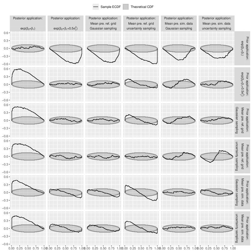
Figure 8: Uniformity check visualisations for Prior-Derived Posterior-Predictive and Prior-Predictive Posterior-Derived Consistency Checks for the Quantity of interest in Case Study I: Prior-Posterior QOI combinations for which the black line remains inside the theoretical cumulatite distribution function (CDF) pass the check.

We compare each of the following prior sample applications to each of the posterior sample applications (results are visualized in Figure 8 on page 8, position statements for the Subfigure rows and columns are given in brackets in the following lists):

(1^st row) $\textsf{E}_{(a),s_{\text{prior}}}$: Version (a) with using $\beta_{0,s_{\text{prior}}}$ and $\beta_{1,s_{\text{prior}}}$,

(2^nd row) $\textsf{E}_{(b),s_{\text{prior}}}$: Version (b) with using $\beta_{0,s_{\text{prior}}}$, $\beta_{1,s_{\text{prior}}}$ and $\sigma_{\gamma,s_{\text{prior}}}$,

(3^rd row) $\textsf{E}_{(c,A,G),s_{\text{prior}}}$: Sample mean of prior prediction on reference grid structure with Gaussian sampling for $\gamma_{j,s_{\text{prior}}}$ from $\gamma_{j,s_{\text{prior}}}\sim\text{Normal}\left(0,\sigma_{\gamma,s_{\text{prior}}}^{2}\right)$,

(4^th row) $\textsf{E}_{(c,A,u),s_{\text{prior}}}$: Sample mean of prior prediction on reference grid structure with uncertainty sampling for $\gamma_{j,s_{\text{prior}}}$,

(5^th row) $\textsf{E}_{(c,B,G),s_{\text{prior}}}$: Sample mean of prior prediction on replicate simulation-data structure with Gaussian sampling for $\gamma_{j,s_{\text{prior}}}$ from $\gamma_{j,s_{\text{prior}}}\sim\text{Normal}\left(0,\sigma_{\gamma,s_{\text{prior}}}^{2}\right)$,

(6^th row) $\textsf{E}_{(c,B,u),s_{\text{prior}}}$: Sample mean of prior prediction on replicate simulation-data with uncertainty sampling for $\gamma_{j,s_{\text{prior}}}$,

vs.

(1^st column) $\textsf{E}_{(a),s_{\text{posterior}}}$: Version (a) with using $\beta_{0,s_{\text{posterior}}}$ and $\beta_{1,s_{\text{posterior}}}$,

(2^nd column) $\textsf{E}_{(b),s_{\text{posterior}}}$: Version (b) with using $\beta_{0,s_{\text{posterior}}}$, $\beta_{1,s_{\text{posterior}}}$ and $\sigma_{\gamma,s_{\text{posterior}}}$,

(3^rd column) $\textsf{E}_{(c,A,G),s_{\text{posterior}}}$: Sample mean of posterior prediction on reference grid structure with Gaussian sampling for $\gamma_{j}$,

(4^th column) $\textsf{E}_{(c,A,u),s_{\text{posterior}}}$: Sample mean of posterior prediction on reference grid structure with uncertainty sampling for $\gamma_{j}$,

(5^th column) $\textsf{E}_{(c,B,G),s_{\text{posterior}}}$: Sample mean of posterior prediction on replicate simulation-data structure with gaussian sampling for $\gamma_{j}$,

(6^th column) $\textsf{E}_{(c,B,u),s_{\text{posterior}}}$: Sample mean of posterior prediction on replicate simulation-data structure with uncertainty sampling for $\gamma_{j}$.

Simulation Study

We repeatedly simulate independently from the above build-up $R=100$ times. For each simulation run, in total $N=500$ observations units and $G=20$ groups are considered.

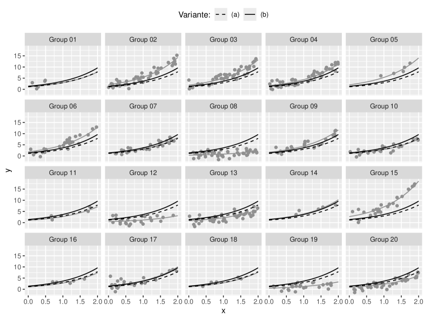
Figure 7: Scatterplot of the data in the 1^st simulation run (Lines visualize the underlying prior sample $\boldsymbol{\theta}_{2}=\left(\beta_{0,2},\beta_{1,2},\sigma_{\gamma_{2}},\gamma_{1,2},\ldots,\gamma_{20,2}\right)^{\top}$). For the duplicate simulation data-set the same values of covariates $x$ and $g$ are re-used.

Figure 7 on page 7 shows a scatter plot for each of the simulated groups in the $r=1$^st simulation run, with additionally also showing $E_{(a),s_{\text{prior}}}$ $E_{(b),s_{\text{prior}}}$ as lines for varying $x\in\left[0,2\right]$.

Figure 12 in Supplement A shows the simulated absolute frequencies for all $20$ groups, $g=1,\ldots,20$, for the first $30$ simulation runs, $r=1,\ldots,30$. Figure 13 in Supplement A shows the SBC-results of the simulation study for Case Study I by uniformity check visualizations according to Säilynoja et al. (2022).

Results

Figure 8 on page 8 shows the results of the simulation study for Case Study I by uniformity check visualizations according to Säilynoja et al. (2022).

We see that $E_{(a),s_{\text{prior}}}$ – results given in the 1^st row of sub-figures – only passes the uniformity check with $E_{(a),s_{\text{posterior}}}$. This means that the conditional perspective is not calibrated with any of the marginal perspectives analysed here.

$E_{(b),s_{\text{prior}}}$ – 2^nd row – only passes the check for $E_{(b),s_{\text{posterior}}}$, and $E_{(c,A,G),s_{\text{posterior}}}$. However, from the posterior application perspective, $E_{(b),s_{\text{posterior}}}$ is calibrated according to $E_{(b),s_{\text{prior}}}$, $E_{(c,A,G),s_{\text{prior}}}$, and $E_{(c,A,u),s_{\text{prior}}}$.

$\textsf{E}_{(c,A,G),s_{\text{prior}}}$ – 3^rd row – passes the check for $E_{(b),s_{\text{posterior}}}$, $E_{(c,A,G),s_{\text{posterior}}}$, and $E_{(c,B,u),s_{\text{posterior}}}$.

$\textsf{E}_{(c,A,u),s_{\text{prior}}}$ – 4^th row – passes the check for $E_{(b),s_{\text{posterior}}}$, $E_{(c,A,G),s_{\text{posterior}}}$, and $E_{(c,A,u),s_{\text{posterior}}}$.

$\textsf{E}_{(c,B,G),s_{\text{prior}}}$ – 5^th row – passes the check for $\textsf{E}_{(c,B,G),s_{\text{posterior}}}$, and $E_{(c,B,u),s_{\text{posterior}}}$ (with slightly crossing the boundaries of the theoretical cumulative distribution function (CDF) region).

$\textsf{E}_{(c,B,u),s_{\text{prior}}}$ – 6^th row – passes the check for $\textsf{E}_{(c,B,G),s_{\text{posterior}}}$, and $E_{(c,B,u),s_{\text{posterior}}}$.

Case Study II: ANOVA decomposition of a bivariate smooth effect surface

This second case study uses a QOI-Check of the form prior-predictive posterior-derived in order to the check univariate ‘main’ effect functions derived of a bivariate smooth effect function as the quantity of interest of a generalized additive models (GAM). The role of the QOI-Check has a stronger focus on providing support for computational implementation of a QOI.

In the R add-on package brms (Bürkner, 2017, 2018), smooth terms, such as the following call s(x, z) for estimation of a bivariate smooth effect ‘surface’, $f\left(x,z\right)$, are implemented using a basis function transformation on the the covariates $x$ and $z$. The brms default here is a Thin Plate Regression Spline basis (Wood, 2003) as implemented by the R add-on package mgcv (Wood, 2011). A design matrix for such smooth terms, denoted $\mathbf{X}_{f\left(x,z\right)}$, is generated on the posterior sampling data $\mathcal{D}$ in order to conduct posterior sampling. For post-estimation calculations on reference data $\mathcal{D}_{a},\mathcal{D}_{b},\ldots$, it would then also be needed to generate such design-matrix objects that not only depend on $\mathcal{D}_{a},\mathcal{D}_{b},\ldots$, but still rely on the distribution of $x$ and $z$ in $\mathcal{D}$ such that the posterior samples are processed correctly on these post-estimation calculation design matrices. To facilitate posterior sampling, brms chooses to use a hierarchical parameterization for s(x, z), leading to design matrix $\mathbf{X}_{f\left(x,z\right)}$ undergoing a sequence of transformations (see Supplement B.1). For post-estimation calculations, the design matrix for the prediction ‘reference grid’ data needs to undergo the exact same transformations, even if the covariate structure of $x$ and $z$ is balanced (very) differently. This leads to a chain of single computational units that needs to checked for correctness during post-estimation calculation of QOIs.

Typically, the interpretation of a bivariate effect is carried on the shared effect surface, $f\left(x,z\right)$, itself. Alternatively, it is also possible to divide $f\left(x,z\right)$ into individual components in order to be able to interpret the two covariate-specific roles of $x$ and $z$ in isolation:

“Sometimes it is interesting to specify smooth models with a main effects $+$ interaction structure such as $\textsf{E}\left(y_{i}\right)=f_{1}\left(x_{i}\right)+f_{2}\left(z_{i}\right)+f_{3}\left(x_{i},z_{i}\right)$ […] for example. Such models should be set up using ti terms in the model formula. For example: y ~ ti(x) + ti(z) + ti(x,z) […]. The ti terms produce interactions with the component main effects excluded appropriately. (There is in fact no need to use ti terms for the main effects here, s terms could also be used.)” (Wood, 2024, page 79)

If we are interested in such an ANOVA decomposition, then we need to implement this post estimation, since a direct estimation of the decomposed effect is not implemented yet in brms. So in order to draw correct conclusions of this decomposition, we need to verify that it is implemented, and interpreted – with respect to an underlying population definition – correctly . It is realized quite quickly that the above steps won’t be implemented within just a few lines of code, and applied researchers therefore need to ‘fight’ Murphy’s law. And at the interpretation stage, we need to answer the question “Which weighting scheme underlies the main effect functions $f_{1}\left(x\right)$ and $f_{2}\left(z\right)$?”. This weighting is an important difference between linear and non-linear effects: For a linear interaction effect, such as in $\text{E}\left(Y\right)=\beta_{1}x+\beta_{2}z+\beta_{3}xz$, it does not make a difference if $x$ and $z$ are uniformly distributed, or not, the average effect for one of the covariates, say $x$, is the same whether one weights according to the distribution of $z$ – as a consequence of the interaction effect $\beta_{3}$ being the same value everywhere in the domain of $z$. For non-linear effects, it of course has an effect if effects are weighted equally in the covariate domain – by using ordinal partial integration –, or if weights are applied that consider the distribution of the covariates. Here, there appears to be no right or wrong, but it is clearly essential that researchers are knowing what their interpretation is based on!

Covariate Structure $\mathcal{D}$ (as used during Posterior Sampling)

The covariates $x$ and $z$ that are plugged into s(x,z) are generated by two independent Beta distributions:

$$\mu_{x}=\frac{\exp\left(\beta_{0,x}\right)}{1+\exp\left(\beta_{0,x}\right)},x\sim\text{Beta}\left(\mu_{x},\phi_{x}\right),\text{ and }\mu_{z}=\frac{\exp\left(\beta_{0,z}\right)}{1+\exp\left(\beta_{0,z}\right)},z\sim\text{Beta}\left(\mu_{z},\phi_{z}\right).$$

Likelihood Model

We use a Normal response model with identity link-function:

$$Y_{i}\sim\text{Normal}\left(\mu_{i},\sigma^{2}\right),\,\,\mu_{i}=\eta_{i},\,\,\eta_{i}=\beta_{0}+f\left(x_{i},z_{i}\right).$$

In the same model, we also estimate the distribution of $x$ and $z$ based on the above data-generating model, i.e. we additionally estimate $\left(\beta_{0,x},\phi_{x},\beta_{0,z},\phi_{z}\right)^{\top}$:

frmla <- bf(x ~ 1, family = Beta(link = "logit")) +

  bf(z ~ 1, family = Beta(link = "logit")) +

  bf(y ~ s(x, z, k = 10), family = gaussian())

Prior Specification

We set the following prior distribution specifications: $\beta_{0,x}\sim\text{Normal}\left(0,0.001^{2}\right)$, $\beta_{0,z}\sim\text{Normal}\left(-1.1,0.001^{2}\right)$, $\beta_{0,y}\sim\text{Normal}\left(0.5,0.1^{2}\right)$, $\beta_{\texttt{s(x,z)},1}\sim\text{Normal}\left(1,0.1^{2}\right)$, $\beta_{\texttt{s(x,z)},2}\sim\text{Normal}\left(-1,0.1^{2}\right)$, $\sigma_{\texttt{s(x,z)}}\sim\text{Normal}_{+}\left(1,0.1^{2}\right)$, $\phi_{x}\sim\text{Normal}_{+}\left(3,0.001^{2}\right)$, $\phi_{z}\sim\text{Normal}_{+}\left(3,0.001^{2}\right)$, $\sigma_{y}\sim\text{Normal}_{+}\left(0.1,0.01^{2}\right)$, where $\text{Normal}_{+}$ denotes the half-normal distribution truncated to only positive real numbers.

Quantity of Interest: ANOVA Decomposition of Bivariate Spline

For a bivariate smooth effect such as used in generalized additive models as provided by the famous R add-on package mgcv (Wood, 2011), we aim to specify a ‘main effects + interaction’ structure post estimation:

$$\text{E}\left(y_{i}\right)=f_{1}\left(x_{i}\right)+f_{2}\left(z_{i}\right)+f_{3}\left(x_{i},z_{i}\right)$$

Here, the ‘main effects’ $f_{1}$ and $f_{2}$ are marginal versions of the ‘bivariate plane’ s(x,z)$, where the effect of the respective other variable is integrated out. The interpretation of $f_{1}$ and $f_{2}$ depends on the form of partial integration:

(a) with

consideration of the empirical distribution of the respective other variable, or

(b) without

consideration of the empirical distribution of the respective other variable.

Prior / Posterior Data-Structure

We set up a data-set in order to for generation of prior or posterior predictions:

• Equidistant grid on $(x,z)$ with uniform weight for each value couple.

• Equidistant grid on $(x,z)$ with univariate distribution weight for $x$ and $z$.

In the code – see Supplement B – I call this reference grid prior prediction. Here, $N=10000$ points are simulated exactly as in the initial data posterior estimation data $\mathcal{D}$ (by using f_generate_xz). However, the valuesfor $x$ are overwritten – sequentially – by fixed values, e.g. $x=0.25$. Then the design matrix issubjected to the transformations described above – and shown / implemented in the code –, parameters are simulated from the prior distribution, and these two parts are then used together to arrive at prior predictions. The sample mean from this is the prior predictive QOI for the respective fixed value of $x$. These valuesare then compared with two versions of the posterior QOI, once with the unweighted calculation of the conditional expectation – on an equidistant grid of $x$ and $z$ –, and once weighted according to the distribution of $z$, which is also estimated using model parameters, as described above.

Simulation Study

We repeatedly simulate independently from the above build-up $R=20$ times.

Results

Figure 10 on page 10 shows the uniformity check for the first main effect $f\left(x\right)$ at a sequence of values for $x$ with univariate distribution weights for $x$. The check is passed at almost any value. Values that don’t pass the check seem practically negligible, also considering the multiple testing attribute of this check.

5 Conclusion

A new approach, the QOI-Check, for checking quantities of interest as derived of a Bayesian probabilistic model was introduced. While Modrák et al. (2023) already introduced SBC with derived quantities, they haven’t focused on any predictive quantities, and therefore not on new reference grid data structures.

It was demonstrated on two application examples (‘Case Studies’) that this check not only leads to trustful post-estimation computations, but also on correct population interpretations of these quantities.

What to QOI-Check, and what not?

Case Study II showcased a quantity of interest that might also be checked based on the derived quantity check presented in Modrák et al. (2023). Case Study I could have also only checked $f\left(\boldsymbol{\theta}_{\text{prior}}\right)$ vs. $f\left(\boldsymbol{\theta}_{\text{posterior}}\right)$, with $f\left(\boldsymbol{\theta}\right)=\exp\left(\beta_{0}+\beta_{1}+0.5\cdot\sigma_{\gamma}^{2}\right)$. In bot cases, however, we won’t gain insights into interpretation with respect to a reference population construction. So as soon as a reference population definition takes a role, the QOI-Check seems worth implementing!

References

Figures

(a) Posterior predictive check, where the comparison is often performed graphically (Gabry et al., 2019, Section 5).

(b) Posterior predictive check for sample statistic $f$.

(c) Holdout predictive check.

Figure 1: Illustration of posterior predictive checks.

Figure 2: Prior Predictive Check.

(a) SBC following Talts et al. (2018), comparing directly a parameter prior sample to the respective parameter posterior samples of that simulation run $r$. The ’cardinal number’ of a set is the number of its elements, e.g. the cardinal number of set $A=\left\{a_{1},a_{2},a_{3}\right\}$ is $3$, denoted $|A|=3$.

(b) SBC following Modrák et al. (2023), comparing a quantity of interest (QOI) based on the prior with the posterior based analogue, where both versions might also depend on $\mathbf{y}_{r}$. As already described in slightly more detail in the caption of Subfigure (a), the ’cardinal number’ of a set is the number of its elements.

Figure 3: Illustration of Simulation-Based Calibration (SBC) check algorithms described in Talts et al. (2018) – shown in Subfigure (a) –, and Modrák et al. (2023) – shown in Subfigure (b).

Figure 4: Prior-Derived Posterior-Predictive Consistency Check.

Figure 5: Prior-Predictive Posterior-Derived Consistency Check.

(a) Primary data structure.

(b) Replicate simulation-data structure $\mathcal{D}_{(A)}$ where an equally balanced vector – of length $N$ – of the primary simulation data-structure for $\mathbf{g}$ is re-used for prediction – vector $\tilde{\mathbf{y}}$ – of $N$ observation units at $x=1$.

(c) Reference grid structure $\mathcal{D}_{(B)}$ where $m$ new observation units are generated, each with $x=1$ and a new grouping variable level that was not included in the $G$ levels present in the posterior estimation data.

Figure 6: Schematic illustration of the estimation data and two post-estimation data structures as used and compared in Application A.

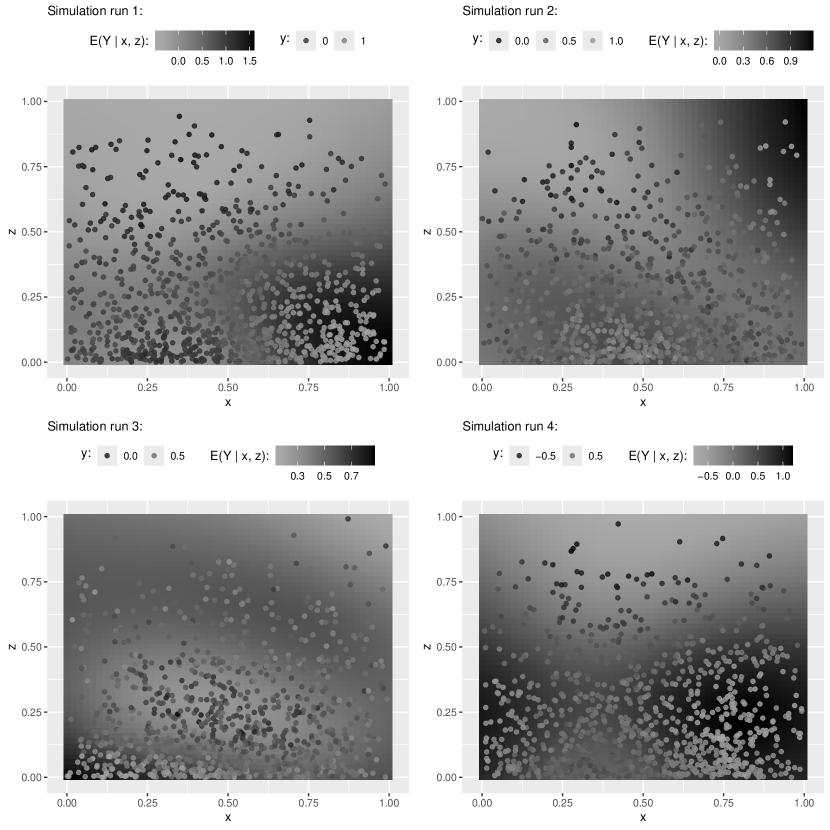
Figure 9: Case Study II: Data and bivariate smooth estimation of the first four simulation runs, $r\in\left\{1,2,3,4\right\}$.

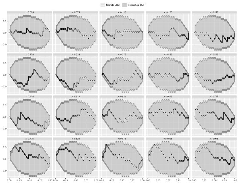
Figure 10: Uniformity check visualisations for Prior-Predictive Posterior-Derived QOI – expectation of y conditional on x with marginalizing out the effect of covariate $z$ – in Case Study II: Prior-Posterior QOI combinations for which the black line remains inside the theoretical cumulatite distribution function (CDF) pass the check.

Supplementary Materials

Supplement 0: Long version of the posterior sampling ‘toy algorithm’

1. Sample values of $\theta_{1},\ldots,\theta_{S}$, from the prior, $p\left(\theta\right)$.

2. For each sampled $\theta_{s}$, $s=1,\ldots,S$, a data-set $\tilde{\mathbf{y}}_{s}$ – with the same dimension as $\mathbf{y}$, usually conditioned on the same covariate data $\mathbf{X}$ – is simulated based on the model, $p\left(Y_{i}\mid\theta\right)$, or $p\left(Y_{i}\mid\theta,\mathbf{X}_{i}\right)$, $i=1,\ldots,n$. This leaves us with $S$ replicated simulations of the original data-set.

3. Define a subset index vector $\mathcal{S}_{\text{sub}}$, which contains a selection of elements of $\mathcal{S}=\left\{1,\ldots,S\right\}$ based on the criterion that $\tilde{\mathbf{y}}_{s}$, $s\in\mathcal{S}$, matches exactly – after practically meaningful rounding for continuous data – the observed data-set $\mathbf{y}$. For example, if $S=5$, and binary ‘matching indicator vector’ $\mathbf{I}=\left(1,0,1,0,1\right)^{\top}$ – where each element is $1$ if the generated data $\tilde{\mathbf{y}}_{s}$ matches the original data, $\mathbf{y}$, and $0$ otherwise –, then $\mathcal{S}_{\text{sub}}=\left\{1,3,5\right\}$.

4. Keep only prior samples $\theta_{s}$, $s\in\mathcal{S}_{\text{sub}}$, and, by this, get the distribution of prior samples that represents our ‘knowledge’ on the likely parameter values that could have generated the observed data vector $\mathbf{y}$.

Rubin (1984) describes this ‘filtering procedure’ as being ‘Bayesianly justifiable’, since it uses the prior distribution to generate hypothetical data and then updates this distribution based on the observed data. This approach aligns with the foundational principles of Bayesian statistics, allowing for coherent and rational inference based on prior knowledge and observed data. However, while valid in theory, it faces the constraint that – in the usually applied range of the examined number, $N$, of observation units, say $N>50$, and most often even much larger – this unstructured search for matching replicated data-sets is much too inefficient, which makes this approach completely impractical when applied in the real-world.

Figure 11 on page 11 shows a sketch for naive posterior sampling – following Rubin (1984, Section 3.1) – in a simulation study with $R$ replications.

Figure 11: ’Naive posterior sampling’ in a simulation study with $R$ replications.

Supplement A: Supplements to Case Study I

Figure 12 on page 12 shows the simulated absolute frequencies for all $20$ groups, $g=1,\ldots,20$, for the first $30$ simulation runs, $r=1,\ldots,30$.

Figure 13 on page 13 shows the SBC-results of the simulation study for Case Study I by uniformity check visualizations according to Säilynoja et al. (2022).

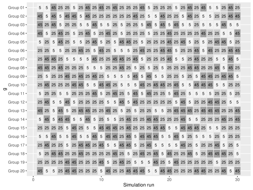
Figure 12: Frequencies of simulated levels of grouping variable $g$ in the first 30 simulation runs.

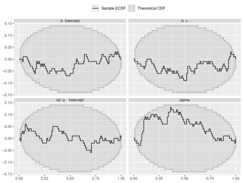
Figure 13: SBC for Case Study I: All single model parameters pass the check.

Supplement A.1: R Code

See website https://uncertaintree.github.io/research/qoi-check.html.

Supplement B: Supplements to Case Study II

Supplement B.1: Smooth Effect Parametrisation in brms

Matrix $\mathbf{X}_{\texttt{s(x,z)}}$ for data $\mathcal{D}$, or $\mathcal{D}_{a}$, $\ldots$, is constructed using mgcv::PredictMat. In order to get to random-effects parameterization, $\mathbf{X}_{\texttt{s(x,z)}}$ is post-multiplied by matrix $\mathbf{U}$, which is a transformation matrix that orthogonalizes the random effect covariance structure. Then, the columns of $\mathbf{X}\mathbf{U}$ are scaled element-wise by the diagonal entries of the matrix $\mathbf{D}$, which contains the square roots of the random effect variances.

The transformed matrix is then split into two components: The component $\mathbf{X}_{\texttt{s(x,z)},1}$ corresponds to the columns of $\mathbf{X}\mathbf{U}$ that are not penalized (those where the entries of $\mathbf{D}$ are zero or not relevant). The ‘penalized’ components are extracted as $\mathbf{X}_{\texttt{s(x,z)},2,l}$, where each of the $L$ columns, $\mathbf{x}_{\texttt{s(x,z)},2,l}$, corresponds to a hierarchical parameter indexed by $l=1,\ldots,L$. The indices for penalization are specified and reordered using internal mechanisms from mgcv::smooth2random to align with the penalty structure of the model.

Thus, the full prediction structure is represented as:

$$\eta=\beta_{0}+\mathbf{X}_{\texttt{s(x,z)},1}\boldsymbol{\beta}_{\texttt{s(x,z)},1}+\sum_{l}\mathbf{x}_{\texttt{s(x,z)},2,l}^{\top}\beta_{\texttt{s(x,z)},2,l},$$

where $\beta_{0}$ is the intercept, $\boldsymbol{\beta}_{\texttt{s(x,z)},1}$ are the parameters for the unpenalized component, and $\beta_{\texttt{s(x,z)},2,l}$ are the parameters for the penalized component.

Using brms, these matrices are then transformed into random effect parameterizations using transformations $\mathbf{U}$ and $\mathbf{D}$. Specifically, $\mathbf{X}$ is post-multiplied by $\mathbf{U}$ and scaled column-wise by $\mathbf{D}$ where applicable. The fixed-effect component $\mathbf{X}_{f}$ is separated from random-effect components $\mathbf{X}_{r}^{(i)}$, which are indexed according to the associated penalization structure. The process ensures that the penalty indices and random effect parameterizations are correctly ordered.

The fixed effects are combined as $\eta_{f}=\mathbf{X}_{f}\boldsymbol{\beta}_{f}$, while the random effects are represented as $\eta_{r}=\sum_{i}\mathbf{X}_{r}^{(i)}\boldsymbol{\beta}_{r}^{(i)}$. The total predictor is expressed as $\eta=\beta_{0}+\eta_{f}+\eta_{r}$, where $\beta_{0}$ is the intercept term. This formulation ensures that the smooth terms and their random-effect parameterizations are fully integrated into the regression model, enabling accurate predictions for new data while maintaining computational efficiency and stability.

Supplement B.2: R Code

See website https://uncertaintree.github.io/research/qoi-check.html.

References

-
Bürkner (2017)
P.-C. Bürkner.
2017. brms: An R Package for Bayesian Multilevel Models
Using Stan.
Journal of Statistical Software.
https://doi.org/10.18637/jss.v080.i01. -
Bürkner (2018)
P.-C. Bürkner.
2018. Advanced Bayesian Multilevel Modeling with the R
Package brms.
The R Journal.
https://doi.org/10.32614/RJ-2018-017. -
Carpenter et al. (2017)
B. Carpenter, A. Gelman, M. D. Hoffman, D. Lee, B. Goodrich, M. Betancourt,
M. Brubaker, J. Guo, P. Li, and A. Riddell.
2017. Stan: A Probabilistic Programming Language.
Journal of Statistical Software.
https://doi.org/10.18637/jss.v076.i01. -
Clark (2004)
J. S. Clark.
2004. Why environmental scientists are becoming Bayesians.
Ecology Letters.
http://dx.doi.org/10.1111/j.1461-0248.2004.00702.x. -
Gabry et al. (2019)
J. Gabry, D. Simpson, A. Vehtari, M. Betancourt, and A. Gelman.
2019. Visualization in Bayesian Workflow.
Journal of the Royal Statistical Society Series A: Statistics in
Society.
https://doi.org/10.1111/rssa.12378. -
Gelman et al. (2013)
A. Gelman, J. B. Carlin, H. S. Stern, D. B. Dunson, A. Vehtari, and D. B.
Rubin.
2013. Bayesian Data Analysis.
Chapman and Hall/CRC.
http://doi.org/10.1201/b16018. -
Gelman et al. (2020)
A. Gelman, A. Vehtari, D. Simpson, C. C. Margossian, B. Carpenter, Y. Yao,
L. Kennedy, J. Gabry, P.-C. Bürkner, and M. Modrák.
2020. Bayesian Workflow.
arXiv:2011.01808.
https://arxiv.org/abs/2011.01808. -
Hoffman and Gelman (2014)
M. D. Hoffman and A. Gelman.
The No-U-Turn Sampler: Adaptively Setting Path Lengths in
Hamiltonian Monte Carlo.
Journal of Machine Learning Research 15(47):1593–1623 2014.
http://jmlr.org/papers/v15/hoffman14a.html. -
Li and Huggins (2024)
J. Li and J. H. Huggins.
2024. Calibrated Model Criticism Using Split Predictive
Checks.
arXiv:2203.15897.
https://arxiv.org/abs/2203.15897. -
Little (1993)
R. J. A. Little.
1993. Post-Stratification: A Modeler’s Perspective.
Journal of the American Statistical Association.
http://doi.org/10.1080/01621459.1993.10476368. -
Modrák et al. (2023)
M. Modrák, A. H. Moon, S. Kim, P. Bürkner, N. Huurre, K. Faltejsková,
A. Gelman, and A. Vehtari.
2023. Simulation-Based Calibration Checking for Bayesian
Computation: The Choice of Test Quantities Shapes Sensitivity.
Bayesian Analysis.
http://dx.doi.org/10.1214/23-BA1404. -
Monnahan et al. (2016)
C. C. Monnahan, J. T. Thorson, and T. A. Branch.
2016. Faster estimation of Bayesian models in ecology using
Hamiltonian Monte Carlo.
Methods in Ecology and Evolution.
http://dx.doi.org/10.1111/2041-210X.12681. -
Moran et al. (2023)
G. E. Moran, D. M. Blei, and R. Ranganath.
2023. Holdout predictive checks for Bayesian model
criticism.
Journal of the Royal Statistical Society Series B: Statistical
Methodology.
https://doi.org/10.1093/jrsssb/qkad105. - Neal (2011) R. Neal. 2011. Handbook of Markov Chain Monte Carlo. CRC Press.
- R Core Team (2024) R Core Team. R: A Language and Environment for Statistical Computing (Version 4.4.1). R Foundation for Statistical Computing 2024.
- Rubin (1984) D. Rubin. 1984. Bayesianly justifiable and relevant frequency calculations for the applied statistician. The Annals of Statistics.
-
Säilynoja et al. (2022)
T. Säilynoja, P.-C. Bürkner, and A. Vehtari.
2022. Graphical test for discrete uniformity and its
applications in goodness-of-fit evaluation and multiple sample comparison.
Statistics and Computing.
http://dx.doi.org/10.1007/s11222-022-10090-6. -
Simmonds et al. (2024)
E. G. Simmonds, K. P. Adjei, B. Cretois, L. Dickel, R. González-Gil, J. H.
Laverick, C. P. Mandeville, E. G. Mandeville, O. Ovaskainen,
J. Sicacha-Parada, E. S. Skarstein, and B. O’Hara.
2024. Recommendations for quantitative uncertainty
consideration in ecology and evolution.
Trends in Ecology & Evolution.
http://dx.doi.org/10.1016/j.tree.2023.10.012. - Stauffer et al. (2009) R. Stauffer, G. J. Mayr, M. Dabernig, and A. Zeileis. 2009. Somewhere over the Rainbow: How to Make Effective Use of Colors in Meteorological Visualizations. Bulletin of the American Meteorological Society.
-
Talts et al. (2018)
S. Talts, M. Betancourt, D. Simpson, A. Vehtari, and A. Gelman.
2018. Validating Bayesian Inference Algorithms with